1

Laboratory Exercises

in

Organic Surface

Chemistry

Kim Daasbjerg Steen Uttrup Pedersen

September 2010

2

Safety

In many of the exercises we will use organic dipolar aprotic solvents like N,N-dimethylformamide ,DMF or acetonitrile, ACN, because they can both solvate organic compounds and ionic compounds like supporting electrolyte or diazonium salts. Dipolar solvents can however rather easy penetrate our skin together with the compounds solvated. It is therefore very important that gloves are used always when these solvents or the filled electrochemical cells are manipulated. The dipolar solvents are also able to penetrate the gloves and they should therefore be removed instantly if they have been contaminated. Wear eye protection at all times in the laboratory and make sure that they stay in front of the eyes.

EXERCISE 1 (Introduction) Voltammetric Investigation of the Reduction of Anthracene

with and without Phenol

Purpose: This exercise serves as an introduction to as well electrochemistry as the electroanalytical technique, cyclic voltammetry, and it is made by all groups simultaneously. During the exercise are examined the fundamental relations between on one hand current and potential and on the other hand concentration and scan rate. A reversible voltammogram is shown, and the characteristic parameters (“peak”-potential, half-“peak”-potential and “peak”-current) are extracted. The modifications of the voltammogram – resulting from the addition of phenol to the cell – are discussed.

Anthracene (M = 178.23 g/mol) Phenol (M = 94.11 g/mol) N.B.! Both compounds are carcinogenic and must, therefore, be treated carefully. This exercise manual is written for the CH-Instruments (CHI 1-3) -Setup

OH

3

Cyclic Voltammetry with CHI-600/CHI-601C. Switch on the potentiostat box and the PC. Enter the program CHI-600 and enter the menu “Setup” → “Hardware Test”. Before starting the general setup has to be correct. Go to “Setup” → “System” and Click “Current Polarity” Cathodic = positive. Make sure that “Save text-file as well” is checked. Go to “Control” → “Cell” → “Active Low” and Stirring 10 and Purge 0. Make sure that “Cell on between Runs” is unchecked. Connect the electrodes and the stirrer (if available) Cyclic Voltammetry: Go now to “Setup” → “Techniques” click “Cyclic Voltammetry”. Now go to “Setup”

→ “Parameters”. The voltage range is determined by “Init E” = “Initial potential”, “Low E” and “High E” are the switch potentials “E[1]” and “E[2]”. “Init P/N” is the direction of the first voltage scan. Reductice scan = “negative” and oxidative scan = “positive”. “Sweep segments” are 2 for each cycle. A normal CV has “Sweep segments”=2 and for multi cycles “Sweep segments”=cycles*2. “Quit time” = 10. “Sensitivity” is like (“Amplif”*1000)-1. “Sensitivity” = 1e-5 is a good starting point which corresponds to “amplif” = 100).

Peak definition: Press and check mark “Diffusive”, “Peak Potential”, “Half Peak Potential” and “Peak Current” . IR-compensation: Go to “Control” → “IR-compensation” or . Click “IR comp mode” = automatic and press “Test” and wait. Click also “IR comp enable” = always. Now return to CV for measurement. If the voltagedrop is still too large (∆Ep > 60 mV) then go back into “Control” → “IR-compensation” and change the value in the “Manual Compensation” and increase the value for the “Resistance (Ohm)” with 5-10 %. Experiment:

4

The CV experiment is started by “Control” → “Run Experiment” or . A plot of the running voltammogram will now be shown. After the experiment the voltammogram will be shown. Press . A cursor system can be used to read E and i directly from the plot. Ep (peak potential) Eh (half-peak potential) and Ah (charge) is measured for all sweeps. The values are already background subtracted. The voltammograms are saved via “File” → “Save as”. The first time in an exercise define a new directory that is used to store all data files. Give each scan a logical name. The text file can now be reprocessed in Sigmaplot. Some of the CHI potentiostats are not equipped with a printer and all plots have to be reprocessed later on another computer.

Chronoamperometry (Exercise 2) and Electrolysis (Exercise 3): Go to “Setup” → “Techniques” click “Chronoamperometry”. Now go to “Setup” → “Parameters”. The voltage range is determined by “Init E” = “Initial potential”, “Low E” and “High E” are the switch potentials “E[1]” and “E[2]”. “Init P/N” is the direction of the first voltage step. Reductice step = “negative” and oxidative step = “positive”. “Number of

steps” is 1 for chronoamperometry and 2 for double potential chronoamperometry.. “Quit time” = 10. “Sensitivity” is like (“Amplif”*1000)-1. “Sensitivity” = 1e-5 is a good starting point which corresponds to “amplif” = 100. It might be necessary to reduce the sensitivity to 1e-4 in order to access current values at time less than 10 ms.

5

Execution (CHI 1-3) 25 ml of 0.1 M TBABF4/DMF electrolytic solution are supplied/distributed together with the electroanalytical cell and working-, counter- and reference-electrodes. Fix the thick test tube with ground stopper (the cell) to the test setup. Transfer 9 ml of the electrolytic solution to the cell. In the electrode holder there is a working electrode – a glassy carbon. The working electrode is a so-called disk electrode with a diameter of 1 mm. Next to it is the counter electrode, which consists of a twisted platinum wire held by a glass tube. The reference electrode consists of a twisted silver wire in a glass tube sealed at one end with a small, porous ceramic plug. This allows a slight contact between the liquid in the reference electrode and the liquid outside – without really mixing. A few grains of tetrabutylammonium iodide are added to the reference electrode and approximately ¼ ml of our standard electrolytic solution is added to the reference electrode. A small magnet is placed in the cell. Check that the electrodes and the stirrer are connected correctly.

Now the cell is ready, but before starting the voltammetric investigation it is necessary to remove oxygen from the solution in the cell. This is done by bubbling nitrogen or argon through the solution for 5-10 min. In the meantime, a standard solution with anthracene can be prepared.

A standard solution is prepared in a measuring flask in such a way that subsequent addition of 1 ml standard solution to the cell will give a concentration of anthracene of 2 mM. Do not add the anthracene solution to the cell now.

Calculate the amount of anthracene to be weighed out for the standard solution.

Anthracene dissolves rather slowly in DMF, and the measuring flasks with the standard solutions are therefore placed in an ultrasonic bath for 5 min to further/facilitate the process.

Switch on the potentiostat box and the PC. Enter the program CHI-600 and enter the menu “Setup” → “Hardware Test”. Before starting the general setup has to be correct. Go to “Setup” → “System” and Click “Current Polarity” Cathodic = positive. Make sure that “Save text-file as well” is checked. Go to “Control” → “Cell” → “Active Low” and Stirring 10 and Purge 0. Make sure that “Cell on between Runs” is unchecked.

6

Go now to “Setup” → “Techniques” click “Cyclic Voltammetry”. Now go to “Setup” → “Parameters”. Insert the voltage range: “Init E” = +0.4, “Low E” = -2.6 and “High E”= +0.4 . “Initial Scan Polarity” is “Negative”. “Sweep Segments” = 2; “Quit time” = 10 and “Sensitivity” = 1e-5 is a good starting point. This is also a good time to find and start the spread sheet program Sigmaplot. We will use this program to depict correlations between different measured characteristica. Start a new spread sheet.

Before recording voltammograms the cell must be connected to the potentiostat. Connect also the wire to the stirrer if such is available. After 5 minutes’ bubbling are you almost ready for the first cyclic voltammogram. In order to be able to measure accurate potentials in the CV-cell it is necessary to compensate for the inevitable IR-loss, which is a potential loss between the surface of the working electrode and the reference electrode. Go to “Control” → “IR-compensation” or . Click “IR comp mode” = automatic and press “Test” and wait. Click also “IR comp enable” = always. Now return to CV for measurement. The CV experiment is started by “Control” → “Run Experiment” or . A plot of the running voltammogram will now be shown. After the experiment the voltammogram will be shown. Press . A cursor system can be used to read E and i directly from the plot. If a printer is available then go to “File” → “Print” (it is also possible to print the voltammogram as a Adobe pdf-file. Finally is the voltammogram saved (“File” → “Save as”. Since this is the first time in this exercise you should define a new directory that is used to store all data files (Create new directory called Exercise1). Give each scan a logical name. The text file can then later be reprocessed in Sigmaplot. Discuss the appearance of the voltammogram of the “blank” electrolytic solution (background).

By use of a syringe now add exactly 1 ml of the anthracene standard and again ventilate the solution for 5 min.. Now adjust the “Low E” in the CV parameters menu to avoid reduction of the electrolytic solution (solvent discharge). Readjust the IR-compensation (“Control” → “IR-compensation” or . Click “IR

Cyclic Voltammetry

-1600 -1400 -1200 -1000 -800 -600 -400 -200 -1.5 -1.0 -0.5

0 0.5 1.0 1.5

Potential/mV

Current/µA

E : -1408.00 mV , I : 0.570 µA , Position :

Mark the beginning of the diffusion controlled region (150mV after Ep) 1:(-440.00mV, -0.1µA) 2:(-839.00mV, -0.1µA)

7

comp mode” = automatic and press “Test” and wait. Click also “IR comp enable” = always). Again record a voltammogram by clicking . Print or save the voltammogram. Discuss the appearance of the anthracene voltammogram. Adjust the “Low E” so that only the first reduction wave of anthracene is shown. Now a reversible voltammogram (see picture) should be shown. Notice the changes when the switch potential is readjusted so that both reduction waves of anthracene are shown. You should also try to make a multiscan by setting the “Sweep Segments” in the CV parameters menu to 4. Run the CV ( ) and print/save the voltammograms. On the basis of these simple voltammograms, make a reaction scheme for the reduction of anthracene. Return to “Sweep Segments” = 2. Try to change the “Scan Rate V/s” to 0.1 V/s, 1.0 V/s, 10 V/s and 100 V/s. Discuss the qualitative data of the voltammograms as regards reaction rates. Now focus on the first reduction wave of anthracene. Adjust the init E, High E and Low E until the scanned potential range is reduced to 0.7 V, the “Init E” = “High E” being approx. 0.4 V less negative than the reduction peak for anthracene. Before the actual measurements we need to define what should be measured. Press and check mark “Diffusive”, “Peak Potential”, “Half Peak Potential” and “Peak Current” . Now run a series of measurements ( ) to determine Ep,1 Eh,1, ip,1 Ep,2, and ip,2 at different scan rates (0.05 V/s, 0.10 V/s, 0.20 V/s ….. 10 V/s). Press the button

. Print/save the voltammograms and input the measured characteristica: scan rate Ep,1, Eh,1, ip,1, Ep,2 and ip,2 into a new Sigmaplot spread sheet. Now add phenol to the cell, so that the phenol- concentration is exactly twice as high as the anthracen-concentration in the cell. That is we have phenol in an excess equal to 2 in relation to the anthracene in the cell. In practice, weigh out the wanted amount of phenol in a specimen tube. Using a glass syringe and needle now transfer a few ml of the cell-solution to the specimen tube where the phenol is quickly dissolved. Return the solvent with the dissolved phenol to the cell. Ventilate the cell for 5 min. with argon or nitrogen. Readjust the IR-compensation. Record ( ) and print/save a voltammogram with scan rate 1.0 V/s. Discuss the changed appearance caused by the phenol. Now gradually increase the scan rate (2.0 V/s, 5.0 V/s …. 100 V/s) and observed the changes. On the basis of these simple voltammograms try to adjust/modify the reaction scheme of the reduction of anthracene. What is the time scale of the reaction? Now determine Ep,1, Eh,1, ip,1, Ep,2 and ip,2 at different scan rates (0.05 V/s, 0.1 V/s, 0.2 V/s, 0.5 V/s and 1.0 V/s). Press the button . Print/save the voltammograms and input the measured characteristica: scan rate Ep,1, Eh,1, ip,1, Ep,2 and ip,2 into a new Sigmaplot spread sheet.

8

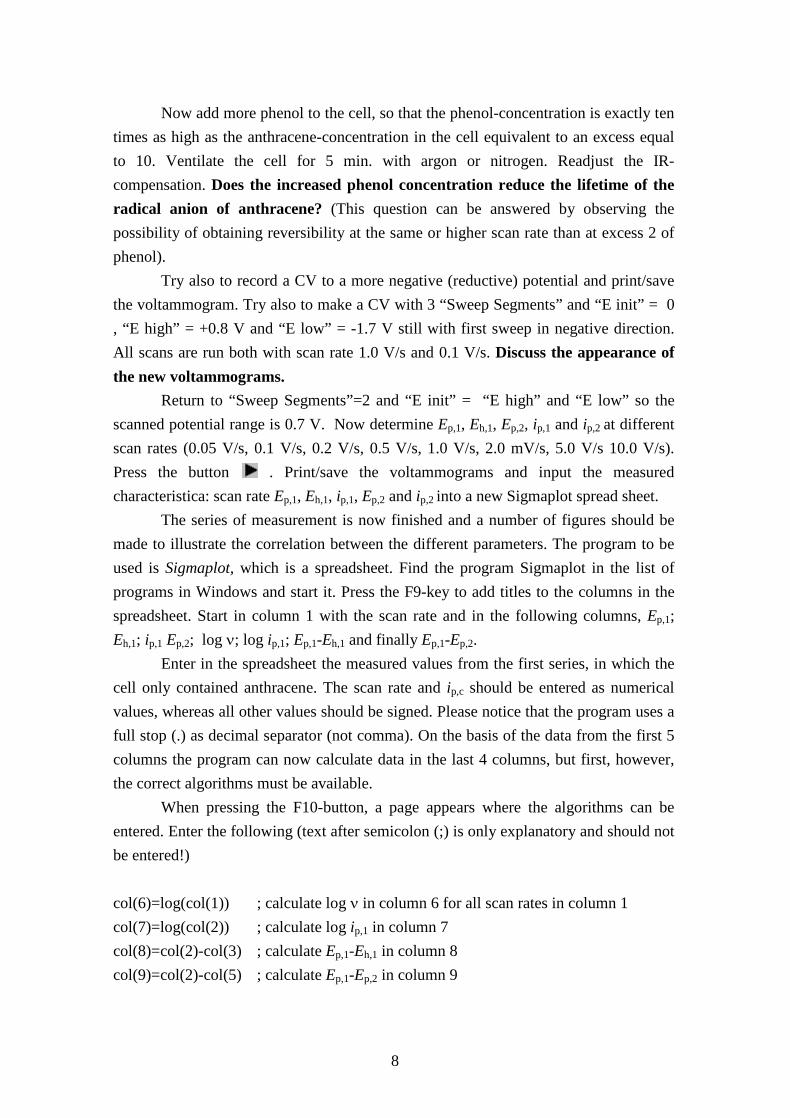
Now add more phenol to the cell, so that the phenol-concentration is exactly ten times as high as the anthracene-concentration in the cell equivalent to an excess equal to 10. Ventilate the cell for 5 min. with argon or nitrogen. Readjust the IR-compensation. Does the increased phenol concentration reduce the lifetime of the radical anion of anthracene? (This question can be answered by observing the possibility of obtaining reversibility at the same or higher scan rate than at excess 2 of phenol).

Try also to record a CV to a more negative (reductive) potential and print/save the voltammogram. Try also to make a CV with 3 “Sweep Segments” and “E init” = 0 , “E high” = +0.8 V and “E low” = -1.7 V still with first sweep in negative direction. All scans are run both with scan rate 1.0 V/s and 0.1 V/s. Discuss the appearance of the new voltammograms. Return to “Sweep Segments”=2 and “E init” = “E high” and “E low” so the scanned potential range is 0.7 V. Now determine Ep,1, Eh,1, Ep,2, ip,1 and ip,2 at different scan rates (0.05 V/s, 0.1 V/s, 0.2 V/s, 0.5 V/s, 1.0 V/s, 2.0 mV/s, 5.0 V/s 10.0 V/s). Press the button . Print/save the voltammograms and input the measured characteristica: scan rate Ep,1, Eh,1, ip,1, Ep,2 and ip,2 into a new Sigmaplot spread sheet. The series of measurement is now finished and a number of figures should be made to illustrate the correlation between the different parameters. The program to be used is Sigmaplot, which is a spreadsheet. Find the program Sigmaplot in the list of programs in Windows and start it. Press the F9-key to add titles to the columns in the spreadsheet. Start in column 1 with the scan rate and in the following columns, Ep,1; Eh,1; ip,1 Ep,2; log ν; log ip,1; Ep,1-Eh,1 and finally Ep,1-Ep,2. Enter in the spreadsheet the measured values from the first series, in which the cell only contained anthracene. The scan rate and ip,c should be entered as numerical values, whereas all other values should be signed. Please notice that the program uses a full stop (.) as decimal separator (not comma). On the basis of the data from the first 5 columns the program can now calculate data in the last 4 columns, but first, however, the correct algorithms must be available. When pressing the F10-button, a page appears where the algorithms can be entered. Enter the following (text after semicolon (;) is only explanatory and should not be entered!) col(6)=log(col(1)) ; calculate log ν in column 6 for all scan rates in column 1 col(7)=log(col(2)) ; calculate log ip,1 in column 7 col(8)=col(2)-col(3) ; calculate Ep,1-Eh,1 in column 8 col(9)=col(2)-col(5) ; calculate Ep,1-Ep,2 in column 9

9

When the algorithms are entered, press “Execute”, and columns 6-9 will be completed. Now different figures are to be constructed. Press the function key F3 to start the construction of a plot. A plot should be constructed of log ip,1 versus log ν (the logarithm of the scan rate), where the measured points are shown (“scatter plot”). Double-click “Scatter Plot” and then “Simple Scatter”. All measuring points are X,Y pair (i.e. log ν,log ip,1), so double-click “X,Y Pair” (i.e. log v, log ip,1). Input to the program that the X-data is in column 6 (log v) and Y-data in Column 7. Click”Finish”, and a plot log ip,1 versus log ν will be shown on the screen. The page-area is the white region on the screen and its size and orientation can be manipulated under the menu “File”→ “Page Setup”→”Orientation” Press “Anvend” (Apply) and then “Ok” All components of the plot can be edited by double clicking on the component (Title, axis, legends, and datapoints). When the appearance of the plot is satisfactory it is time to determine the relation between ip,1 and ν via the log-log plot.. Choose the menu ”Statistics”→ ”Linear Regression.”. Mark ”Each Curve” and ”Extend To Axes” and press ”Anvend” (apply). Go to “Results” and high-light the three lines with the results of the linear regression (b[1], b[0] and r2). Press “Copy” (or Ctrl + C). Click ”Ok”. Now paste the correlation results into the figure by Ctrl + V. The new object can be edited and moved on the plot as you may wish. Print the plot. What is the relation between the ’peak-current, ip,1 , and scan rate, ν ? Make three other plots showing Ep,1 versus log v, Ep,1-Eh,1 versus log v and finally Ep,1-Ep,2 versus log v. Discuss the relations between the measured characteristics and the scan rate. Input now the data from the measurements with phenol in excess 2 and 10 and construct similar plots for these measurements. Notice however that the measurement of Ep,2 and ip,2 is not relevant here because the anodic peak is absent at certain scan rates. Discuss again the relation between the measured characteristics and the scan rate. Finally, we will focus on the effect of the measured characteristics and the concentration of phenol. Input in a new data sheet in column 1 the three phenol concentrations (0 mM, 4 mM and 20 mM). Input in columns 2-4 the measured Ep,1, Eh,1 and ip,1 for scan rate 0.1 V/s and in column 5-7 the measured Ep,1, Eh,1 and ip,1 for scan rate 1.0 V/s. Construct plots there show the relation between Cx (Cx is the concentration of phenol) and Ep,1, Ep,1-Eh,1 and ip,1. Discuss the relations between the measured characteristics and the concentration of phenol.

10

EXERCISE 2 Absolute determination of n and D for the reduction of

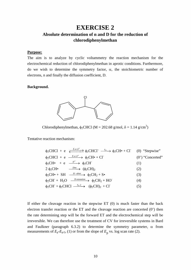
chlorodiphenylmethan Purpose: The aim is to analyze by cyclic voltammetry the reaction mechanism for the electrochemical reduction of chlorodiphenylmethan in aprotic conditions. Furthermore, do we wish to determine the symmetry factor, α, the stoichiometric number of electrons, n and finally the diffusion coefficient, D. Background.

Chlorodiphenylmethan, φ2CHCl (M = 202.68 g/mol, δ = 1.14 g/cm3

)

Tentative reaction mechanism: φ2CHCl + e , , oE kα→← φ2CHCl-. clk→ φ2CH• + Cl- (0) “Stepwise”

φ2CHCl + e , , oE kα→ φ2CH• + Cl- (0’) “Concerted” φ2CH• + e

'oE→ φ2CH- (1) 2 φ2CH• Dim→ (φ2CH)2 (2) φ2CH• + SH H abstr−→ φ2CH2 + S• (3) φ2CH- + H2O Pr otonation→ φ2CH2 + HO- (4) φ2CH- + φ2CHCl 2NS→ (φ2CH)2 + Cl- (5) If either the cleavage reaction in the stepwise ET (0) is much faster than the back electron transfer reaction or the ET and the cleavage reaction are concerted (0’) then the rate determining step will be the forward ET and the electrochemical step will be irreversible. We can therefore use the treatment of CV for irreversible systems in Bard and Faulkner (paragraph 6.3.2) to determine the symmetry parameter, α from measurements of Ep-Ep/2, (1) or from the slope of Ep vs. log scan rate (2).

Cl

11

α =/ 2

1.85

p p

RTF E E−

= / 2

47.7( )a p pn E E−

(1)

α = ln2 p

RT dF dE

ν− ⋅⋅

= -0.02958· log

p

ddE

ν (2)

The stoichiometric number of electrons can be determined by several ways. The most popular method is by coulometry and exhaustive preparative electrolysis. It can however be problematic to use these n-values obtained from coulometry in the interpretation of the cyclic voltammograms because the time scale and the reaction conditions are so different. In coulometry the timescale is perhaps 1 hour and the reaction layer is the bulk of the cell whereas in CV the timescale can be less than a second and the reaction layer is a fraction of a mm from the electrode surface. Give examples of mechanisms, where the stoichiometric number of electrons, n measured by coulometry and CV would be different. Another very popular method used to determine n values in CV is to add a ”standard” compound (typical ferrocene where n=1) to the same CV-cell and then directly compare peak currents between the investigated system and the standard. However, this comparison is based on the assumption that the diffusion coefficients of the investigated compound and the standard are equal, which can be difficult to know in advance. Beside this one need also to take into account that heterogeneous and homogeneous chemical reactions can influence the shape and height of the voltammetric wave. The method is therefore not always very precise. If, however, measurements from a transient technique, with planar diffusion and itr ∝ n D1/2 are combined with measurements by steady-state voltammetry with spherical diffusion and iss ∝ n D then D can be eliminated from the considerations by using 2 /tr ssi i n∝ . If different electrodes are used for the transient and the steady-state

measurements then the measured currents needs to be normalized for the effect of the electrode area. We can however avoid electrode area normalization if the same measurements with the same electrodes are conducted on a standard compound like ferrocene with known n and D. Execution (CHI 1-3 in lab. 431) 50 ml 0.1 M TBABF4/DMF dried electrolytic solution are supplied. A standard solution is prepared in a 10 ml measuring flask by addition of precisely 35.5 µl φ2CHCl (M = 202.68 g/mol, d = 1.14 g/ml) and filling up with 0.1 M TBABF4/DMF. Transfer 9 ml of 0.1 M TBABF4/DMF to the cell and include a small magnet for

12

stirring. The Plastic-stopper should include one 1.0 mm (diameter) glassy carbon working electrode (disc), one twisted platinum wire counter electrode, one Ag+,I- / Ag reference electrode (Se exercise 1 for the details concerning the reference electrode) and finally one cannula for bubbling argon through the solution in order to remove oxygen. Connect all electrodes to the potentiostat and purge the electrolyte solution with argon for 5-10 min.

While waiting switch on the potentiostat box and the PC. Enter the program CHI-600 and enter the menu “Setup” → “Hardware Test”. Before starting the general setup has to be correct. Go to “Setup” → “System” and Click “Current Polarity” Cathodic = positive. Make sure that “Save text-file as well” is checked. Go to “Control” → “Cell” → “Active Low” and Stirring 10 and Purge 0. Make sure that “Cell on between Runs” is unchecked. Go now to “Setup” → “Techniques” click

“Cyclic Voltammetry”. Now go to “Setup” → “Parameters”. Insert the voltage range: “Init E” = 0.0, “Low E” = -2.6 and “High E”= 0.0 . “Initial Scan Polarity” is “Negative”. “Scan Rate” = 1.0 V/s, “Sweep Segments” = 2; “Quit time” = 10 and “Sensitivity” = 1e-5 is a good starting point. Connect the electrodes and the stirrer (if available).

After 5 minutes’ bubbling compensate for the inevitable IR-loss. Go to “Control” → “IR-compensation” or . Click “IR comp mode” = automatic and press “Test” and wait. Click also “IR comp enable” = always. Click to record the first cyclic voltammogram of the electrolytic solution without chlorodiphenylmethan. This voltammogram is your “blank” or background voltammogram. Print/save the voltammogram by entering “File” menu and choose “Print” or “Save as”. Add now 1 ml of the φ2CHCl-standard solution by syringe and ventilate again the solution with Argon for 5 min. Hereafter readjust the IR-compensation and click to record the CV of chlorodiphenylmethan. Print/save the voltammogram. Adjust the potential range (“E init” = “High E” and “Low E”) to 500 mV before and after the

13

reduction wave peak for chlorodiphenylmethan. Record and print/save the focussed voltammogram. Change now “Scan Rate to 0.1 V/s, 1.0 V/s, 10.0 V/s and 100 V/s). It is probably necessary to change the “Sensitivity” here. Increase the sensitivity if the reduction peak is cut off and decrease the sensitivity if the peaks are too small. Discuss the qualitative informations obtained from the voltammograms. Is the reduced form of chlorodiphenylmethan stable? Give a maximum life time of φ2CHCl•-. We will now measure the peak characteristics of the reduction wave for benzyl chloride. Enter “Sweep Segments” = 1. Before the actual measurements we need to define what should be measured. Press and check mark “Diffusive”, “Peak Potential”, “Half Peak Potential” and “Peak Current” . Now record ( ) a series of measurements to determine Ep, Eh and ip at different scan rates (0.05 V/s, 0.1 V/s, 0.2 V/s ….. 10.0 V/s). For each scan rate input in a Sigmaplot spreadsheet Scan Rate (ν), Ep, Eh, ip and calculate (or let Sigmaplot do) ip⋅ν-1/2

Use the results of the measurements to calculate α-values from eqns. (1) and (2). A table of α-values can be made via eqn. (1) and one overall value can be calculated from eqn. (2). The latter requires a plot of Ep vs log scan rate and a linear regression analysis to obtain the slope. Find the relation between ip and ν

via a logarithmic plot.

.

The stoichiometric number of electrons in the reduction of φ2CHCl will be determined relative by addition of a standard, ferrocene, with a one electron oxidation process. Prepare a ferrocene standard solution with 37.2 mg ferrocene in 10 ml 0.1 M TBABF4/DMF in a measurement flask. Add 1 ml of the ferrocene standard solution by syringe to the cell. Ventilate the cell again with Argon for 5 min and readjust the IR-compensation. Measure ( ) ip for φ2CHCl at ν[1] = 1.0 V/s. Adjust now the ”Initial E” = 0 V = “Low E” and ”High E ” = +1.0 V. “Init P/N” should here be positive. Record a new voltammogram of the oxidation of ferrocene by pressing . Focus again the potential range around the oxidation wave and print/save the voltammogram. Measure ( ) ip for the oxidation wave of ferrocene. Assume that ferrocene and φ2CHCl have equal diffusion coefficients (DF = DB) and n for ferrocene is 1 (nF = 1) and calculate nB for φ2CHCl. Remember that the voltammogram for ferrocene is reversible and use eqn. (3) and eqn. (4) for the irreversible reduction of φ2CHCl. Use the α-value determined previously. 5 3/ 2 1/ 2 * 1/ 2

, (2.69 10 )p rev F F Fi n AD C ν= ⋅ (3) Similar to eqn. 6.2.19 in B&F

5 1/ 2 1/ 2 * 1/ 2, (2.99 10 )p irrev B B Bi n AD Cα ν= ⋅ ⋅ (4) Similar to eqn. 6.3.8 in B&F

14

It can often be difficult to know if diffusion coefficients will be similar or not and in the following section will we perform a series of experiments combining transient (Chronoamperometry) and steady-state (voltammetry) that will allow us to skip this assumption and to determine absolute n and D values for φ2CHCl. All experiments will be made in the present cell but we will change working electrode later before the steady-state voltammetry.

Go to the menu "Techniques" and choose "Chronoamperometry". Use the peak potential for ferrocene measured in the previous section. The ”Init E” = “Low E” should be equal to the measured peak potential subtracted 300 mV (Ep,Fer -300) and “High E” should be Ep,Fer + 300. Set “Init P/N” = Positive and “Number of Steps” = 1. Set “Pulse Width” = 1.0 sec. Adjust “Sensitivity” to 1e-5. Finally disable the IR-compensation (Go to “Control” → “IR-compensation” or . Uncheck “IR Compensation for Next Run” Press the button . The curve shown should follow the Cottrel equation, where the

current decrease as 1time

. Save the file and import the time-current values into

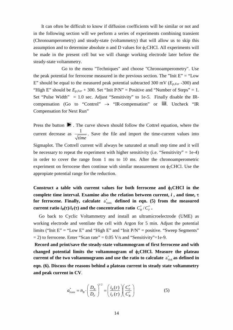
Sigmaplot. The Cottrell current will always be saturated at small step time and it will be necessary to repeat the experiment with higher sensitivity (i.e. “Sensitivity” = 1e-4) in order to cover the range from 1 ms to 10 ms. After the chronoamperometric experiment on ferrocene then continue with similar measurement on φ2CHCl. Use the appropiate potential range for the reduction. Construct a table with current values for both ferrocene and φ2CHCl in the complete time interval. Examine also the relation between current, i , and time, τ for ferrocene. Finally, calculate a trans

∗ defined in eqn. (5) from the measured current ratio iB(τ)/iF(τ) and the concentration ratio * */B FC C .

Go back to Cyclic Voltammetry and install an ultramicroelectrode (UME) as working electrode and ventilate the cell with Argon for 5 min. Adjust the potential limits (“Init E” = “Low E” and “High E” and “Init P/N” = positive. “Sweep Segments” = 2) to ferrocene. Enter “Scan rate” = 0.05 V/s and “Sensitivity”=1e-9. Record and print/save the steady-state voltammogram of first ferrocene and with changed potential limits the voltammogram of φ2CHCl. Measure the plateau current of the two voltammograms and use the ratio to calculate a disk

∗ as defined in

eqn. (6). Discuss the reasons behind a plateau current in steady state voltammetry and peak current in CV.

1/ 2 *

**

( )( )

B B Ftrans B

F F B

D i Ca nD i C

ττ

= ⋅ =

(5)

15

*

,**

,

ss BB Fdisk B

F ss F B

iD Ca nD i C

= ⋅ =

(6)

Only a* based on measurements of the same time scale can be combined in eqns. (7) and (8).

* 2

*

( )transB

disk

ana

= (7)

2*

*disk

B Ftrans

aD Da

= ⋅

(8)

The time scale of a steady-state experiment is roughly τdisk= r2/DF, where r is the

radius of the UME and DF is the diffusion coefficient of ferrocene, which in DMF is 1.1⋅10-5 cm2s-1. Calculate nB and DB for φ2CHCl from eqns. (7) and (8) and discuss the time window valid for this estimation of nB. Compare the two estimations of nB and comment on the validity of the assumption of DB = DF used in the first method.

Exercise 3

Electrochemical grafting of 4-nitrobenzenediazonium salt Purpose

The purpose of this exercise is to introduce the electrochemically assisted grafting of

aryldiazonium salts and compare electrochemical behaviour of the grafted film with the

free analogue. The grafted films will be characterized by electroanalytical techniques.

Nitrobenzene (M = 123,11 g/mol, δ = 1.196 g/mL)

NO2

16

N.B.! The compound is carcinogenic and must, therefore, be treated carefully. Background

Electrochemical reduction of aryldiazonium salts at a conducting surface such as glassy

carbon to the corresponding diazenyl radicals is a facile process followed by a fast

expulsion of dinitrogen to give aryl radicals (Scheme 1).1,2

strong C-C bonds opens up the possibility of immobilizing thin but resistant organic

layers on top of the surface. Unfortunately for some aplication will continued

production of aryl radicals lead to their attack on already grafted molecules in a

Gomberg type reaction which leads to multilayers possibly resulting in mushrooms

shapes on the electrode surface.

As a result the reactive aryl

radicals will be formed at the close vicinity of the surface, thus allowing them to attack

the π system of the surface carbon framework. The resultant formation of covalent and

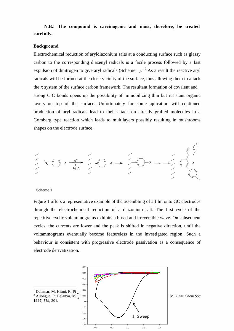
Figure 1 offers a representative example of the assembling of a film onto GC electrodes

through the electrochemical reduction of a diazonium salt. The first cycle of the

repetitive cyclic voltammograms exhibits a broad and irreversible wave. On subsequent

cycles, the currents are lower and the peak is shifted in negative direction, until the

voltammograms eventually become featureless in the investigated region. Such a

behaviour is consistent with progressive electrode passivation as a consequence of

electrode derivatization.

1 Delamar, M; Hitmi, R; Pinson, J; Savéant, J-M. J.Am.Chem.Soc 1992, 114, 5883. 2 Allongue, P; Delamar, M; Desbat, B; Fagebaume, O; Hitmi, R; Pinson, J; Savéant, J-M. J.Am.Chem.Soc 1997, 119, 201.

XN2 Xe

N2 (g)

X X

X

X

Scheme 1

E / V vs SCE

-0.4 -0.2 0.0 0.2 0.4

i / µ

A

-1.8

-1.6

-1.4

-1.2

-1.0

-0.8

-0.6

-0.4

-0.2

0.0

0.2

1. Sweep

17

A) Cyclic voltammetry of nitrobenzene in aprotic solvent Use the same procedure as in exercise 1 to make an electroanalytical cell with 2 mM nitrobenzene in 10 ml 0.1 M TBABF4/DMF (remember to run a background voltammogram with 9 mL 0.1 M TBABF4/DMF). The cell is mounted with a platinum

counter electrode, a Ag/AgI reference electrode and a 1mm glassy carbon working electrode. A small magnet is placed in the cell. Record CV-voltammograms (from 0 V to -2.6 V at ν = 1 V/s) of the background and with the 2 mM nitrobenzene. Print/save the voltammograms and discuss the electrochemistry of nitrobenzene. Adjust the potentials so that only the first reduction wave of nitrobenzene is shown. Now a reversible voltammogram (see picture) should appear. Notice the changes that take place if the switch potential is readjusted so that both reduction waves of nitrobenzene are shown. You should also try to make a multiscan by setting the “Sweep Segments” equal to 4 and print/save the voltammograms. On the basis of these simple voltammograms a reaction scheme is proposed for the reduction of nitrobenzene. Determine the standard potential as the mid-point of the cathodic and anodic peak potentials. “Sweep Segments” is returned to 2. Go to “Control” → “IR-compensation” or . Click “IR comp mode” = automatic and press “Test” and wait. Click also “IR comp enable” = always. Try now to change the “Scan Rate το (0.1 V/s, 1.0 V/s, 10.0 V/s and 100 V/s). Discuss qualitatively the voltammograms and the reaction rates. Focus now on the first reduction wave of nitrobenzene. Adjust the initial and final potential until the scanned potential range is reduced to 700 mV, the starting potential being approx. 400 mV less negative than the reduction peak for nitrobenzene. Run ( ) a series of measurements to determine Ep,1, Eh,1, ip,1, Ep,2 and ip,2 at different scan rates (0.05 V/s, 0.1 V/s, 0.2 V/s ….. 10.0 V/s).

Figure 1. Cyclic voltammograms of 2 mM solution of a diazonium salt recorded at a sweep rate of

0.1 V s-1 in 0.1 M Bu4NBF4/acetonitrile.

18

Enter in the spread sheet the measured values from the first series, in which the cell only contained nitrobenzene and present the electrochemical characteristics (ip,1, vs scan rate, Ep,1 vs scan rate, Ep,1- Eh,1 vs scan rate.

B) Cyclic Voltammetry of nitrobenzene in 0.1 M H2SO4.

Transfer 9 ml of 0.1 M H2SO4 aqueous solution to the electrochemical cell. Insert the

same working electrode and counter electrode as before. The reference electrode is for

aqueous solution a saturated calomel electrode (SCE) connected to the cell via a

saturated KCl salt bridge. A small magnet is placed in the cell.

Bubble nitrogen or argon through the solution for 5-10 min. Prepare a new

standard solution of nitrobenzene in 0.1 M H2SO4 in a measuring flask in such a way

that subsequent addition of 1 ml standard solution to the cell will give a concentration

of nitrobenzene of 2 mM. Do not add the nitrobenzene solution to the cell yet.

As before the CV of the “blank” 0.1 M H2SO4 solution is recorded. Discuss the

voltage range available (voltage before medium discharge) and compare it with the

situation for the TBABF4/DMF solution. Add 1 mL of the aqueous standard of

nitrobenzene and bubble with nitrogen or argon. Record the cyclic voltammogram from

+0.7 V to -1.0 V vs SCE using a scan rate of 0.1 V s-1. Save the data for the

voltammogram in a new spreadsheet in Sigmaplot. Record and save the next 4

voltammograms in separate columns in the same Sigmaplot spreadsheet. Construct a

figure in Sigmaplot that shows all ten voltammograms (Create a graph → Scatter plot

→ Multiple straight lines→ X,Y pairs).

Perform also 2 CV cycles and try to add a microscopic amount of

nitrosobenzene directly to the cell. Discuss the possible mechanism taking the

following reactions into account.

4H + 4e

NHOHNO2 NH22H + 2e

H2O H2O

NHOH NO

-2H + -2e2H + 2e

C) Electrochemically assisted grafting of 4-nitrobenzene diazonium tetrafluoroborate

19

4-Nitrobenzenediazonium tetrafluoroborate (M = 237 g/mol) N.B.! The compound is carcinogenic and must, therefore, be treated carefully.

The electrografting of arenediazonium salts will be made in an electrolytic solution of

acetonitrile (CH3CN) because hydrogen atom abstraction in this solvent is slower than

in DMF. Acetonitrile should be used as solvent in cell and in the reference electrode.

Prepare 25 ml of 0.1 M TBABF4/CH3CN electrolytic solution and transfer 10 ml to the

electrochemical cell. Insert the same 1 mm glassy carbon working electrode and counter

electrode as before. The reference electrode is again a silver wire but the solution is

now the acetonitrile electrolyte solution with a few grains of tetrabutylammonium

iodide. A small magnet is placed in the cell and the solution is bubbled with N2 or Ar

for 5 min. Record the first cyclic voltammogram from +0.8 V to -0.2 V vs Ag/AgI with

a scan rate of 0.1 V/s. Save the data for the voltammogram in a spread sheet in

Sigmaplot. Disconnect the cell and add 4.7 mg 4-nitrobenzenediazonium

tetrafluoroborate in order to obtain a 2 mM concentration.

Record and save the next 5 voltammograms in separate columns in the same Sigmaplot

spread sheet. Construct a figure in Sigmaplot that shows all voltammograms (Create a

graph → Scatter plot → Multiple straight lines→ X,Y pairs). Discuss the features of the

voltammograms recorded for nitrobenzene in aprotic and protic solvent and for the

grafting of 4-nitrobenzene diazonium tetrafluoroborate. Save this electrode as 4-

nitrophenyl-grafted number 1.

Graft now 4 other GC electrodes by Chrono Coulometry. Go to the menu point

“Techniques” and to the subpoint “Chronocoulometry”. Fill out the parameters “Init E

= +0.8 V = “High E” and “Low E” = -0.2 V. “Number of Steps” = 1 and “Pulse Width”

= 300 sec. “Sensitivity” = 1e-4. Do not touch the other buttons except the . Mark

these four electrodes with 2-5.

D) Cyclic voltammetry of grafted 4-nitrobenzene in aprotic conditions

NO2

N2+F4B-

20

Prepare the cell with 10 mL 0.1 M TBABF4/DMF and the magnet. Insert the counter

electrode and the Ag/AgI reference electrode from the first experiment (Part A). Start

with the 4-nitrophenyl-grafted electrode number 1. Remove oxygen from solution by

bubbling with N2 or Ar and record a “double cycle cyclic voltammogram” from +0.2 V

to -1.1 V and print/save the voltammogram. Import the data in a Sigmaplot spread

sheet. The coulombs Q used for the reduction of grafted 4-nitrobenzene can be

determined in the CHI-600 program by means of the menu point Ah (Press and

check mark “Peak area”) or ask the instructor to help you do the integration in

Sigmaplot,

The surface coverage of grafted 4-nitrobenzene, Γ, can be calculated from

eqn. (1) on the assumption that each molecule is reduced by 1 electron.

Q = n⋅F⋅A⋅Γ (1)

The parameter n is the number of electrons transferred and A is the electrode area.

Carry out the same integration procedure on the oxidation wave and calculate Γ. If

possible also the reduction and oxidation peaks similarly on the second cycle are

integrated.

Discuss the voltammograms recorded and compare them with the voltammogram

recorded for nitrobenzene in solution during part A.

E) Cyclic voltammetry of grafted 4-nitrobenzene in acidic conditions

Prepare a cell containing 10 mL of 0.1 M H2SO4 with a counter electrode and a

KCl-Saltbridge/SCE reference electrode. Use the GC electrode marked with “2” as the

working electrode and remove oxygen from the solution. Record a “double cycle”

cyclic voltammogram from +0.6 V to -0.9 V and plot the voltammogram. Save the data

in a Sigmaplot spread sheet. Save also the data in an ascii-file (“Data”→”export to

asciifile”). Integrate the reduction peak and the oxidation peak for the hydroxylamine.

Calculate Γ for grafted 4-nitrobenzene on the assumption that the reduction peak arises

from a combination of 6e reduction to the 4-anilin and 4e reductions to the N-phenyl-

hydroxylamine. Compare the result with the surface coverage previously determined in

TBABF4/DMF.

21

4H + 4e

NHOHNO2 NH2

2H + 2e

H2O H2O

NHOH NO

-2H + -2e2H + 2e

Show that Γ can be calculated as the sum of the integrated reduction peak of nitrophenyl and the oxidation peak of hydroxylaminophenyl divided by 6. F) Qualitative test of the robustness of the electrografted 4-nitrophenyl film

One of the great advantages of the electrografting procedure using diazonium salts is

that the attachment of organic molecules to the surface goes through a covalent linkage.

To test the durability of this linkage the modified electrodes are exerted to extreme

conditions involving extensive heating and/or ultrasonication in various solvents. After

each treatment the electrochemical properties of the electrodes are tested and the

surface concentrations measured.

Use the cell prepared in section D and electrodes 3-5 prepared in section C. Scan from -

0.2 V to -1.1 V vs Ag/AgI with a high scan rate. i.e. 10V/s. Determine for each

electrode the surface concentration, Γ, by the procedure used in section C. After this is

electrode 3 placed in the oven at 60 OC for 15 min, electrode 4 is ultrasonicated in

acetonitrile for 15 min and finally is electrode 5 washed with acetone. The surface

coverages of the three electrodes 3-5 are subsequently measured by CV and compared

with the values before the treatment.

22

Exercise 4

Qualitative test of aryldiazonium electrografted films with redox

probes and contact angle measurements Purpose

The aim of this part of the exercise is to illustrate how the electron transfer to solution

based redox probes in solution can be used to describe the blocking properties of the

grafted film. The hydrophilic/hydrophobic interaction of different grafted films with

water is furthermore described by contact angle measurements.

Background

Cyclic voltammetry of solution-based redox probes at grafted electrode surfaces gives a

good measure of the blocking properties of the grafted film. Blocking properties cover

effects of film thickness/pin holes, electrostatic and hydrophobic interactions. In this

part of the exercise we will use two different redox probes to test the surface conditions.

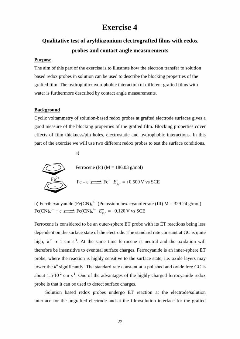
a) Ferrocene (fc) (M = 186.03 g/mol) Fc – e →← Fc+ 0.500o

FcE + = + V vs SCE

b) Ferrihexacyanide (Fe(CN)63- (Potassium hexacyanoferrate (III) M = 329.24 g/mol)

Fe(CN)63-. + e →← Fe(CN)6

4- 0.120oFc

E + = + V vs SCE Ferrocene is considered to be an outer-sphere ET probe with its ET reactions being less

dependent on the surface state of the electrode. The standard rate constant at GC is quite

high, 'ok ≈ 1 cm s-1. At the same time ferrocene is neutral and the oxidation will

therefore be insensitive to eventual surface charges. Ferrocyanide is an inner-sphere ET

probe, where the reaction is highly sensitive to the surface state, i.e. oxide layers may

lower the ko significantly. The standard rate constant at a polished and oxide free GC is

about 1.5⋅10-2 cm s-1. One of the advantages of the highly charged ferrocyanide redox

probe is that it can be used to detect surface charges.

Solution based redox probes undergo ET reaction at the electrode/solution

interface for the ungrafted electrode and at the film/solution interface for the grafted

Fe2+

-

-

23

electrode. If the grafted film is insulating and uniform without pinholes or permeability

the effect of the film will be to decrease ko with the distance between the redox center

and the electrode surface. The tunnelling parameter, β, is dependent on the nature of the

electron transport through the film. If the electron tunnels in one step (coherent

tunnelling process) directly through space then an exponential decrease of ko will be

observed and β will be small (∼ 0.2 Å-1). Under such circumstances even thin films (d

∼1 Å) will effectively prevent the ET to the redox probe and only redox probes with

high ko at the bare electrode will be active.

If the transport of electrons in the film takes place by hopping through bonds to

redox sites in the film the rate will be inversely proportional to the distance. The

insulating properties will then be dependent on the exact nature of the film in terms of

saturated bonds or conjugated bonds.

Also the film surface properties like charge and hydrophilicity will be important.

If a net surface charge on the film can be generated i.e. by protonation or deprotonation

of a neutral molecule then a charged redox probe like ferrihexacyanide may be

attracted/repelled. Hydrophilic groups on the film surface will interact with the redox

probes and the counter ions and change the distance of the redox probe to the film

surface.

The properties of this surface layer can be controlled through appropriate

selection of the substituent X at the aryl group. In this exercise will we use X = COOH,

NO2, and H to reveal the extent by which the hydrophilicity/hydrophobicity of the

surface as deduced from the shape of a water drop placed on the surface is affected by

the nature of the substituent.

Procedure

1) Prepare two cells; one with 2 mM ferrocene in 0.1 M TBABF4/CH3CN and another

with 2 mM K3Fe(CN)4 in 0.1 M phosphate buffer (pH = 7). Both cells are equipped

with freshly polished 1 mm glassy carbon working electrode and a platinum wire

counter electrode. A Ag/AgI reference electrode is used in the 0.1 M

TBABF4/CH3CN and a saturated calomel electrode with a KCl salt bridge is used in

the phosphate buffer.

2) The electrochemical properties of six glassy carbon electrodes (freshly polished) are

tested towards the two solution redox probes (2 mM solutions), ferrocene and

K3Fe(CN)4, by recording cyclic voltammograms at a sweep rate of 0.1 V s-1. All

recorded voltammograms are saved and printed.

24

3) The next step concerns the electrografting of the glassy carbon surfaces (3 × 2 sets

of electrodes) using the three aryldiazonium salts (X = COOH, NO2, and H). Prepare

three cells with 2 mM of the relevant aryldiazonium salts in 0.1 M TBABF4/CH3CN.

We will a potentiostatic electrolytic grafting. All solutions are carefully deaerated

with argon before use. From the recording of a single cyclic voltammetric sweep

(print and save) the appropriate electrolysis potential is selected as E = Ep,c – 200

mV, where Ep,c is the cathodic peak potential. The electrografting (i.e. surface

modification) is then carried out for 5 minutes in Chronocoulometry (see exercise 3)

by adjusting the electrolysis potential. At the same time the solution is stirred. For

each diazonium salt two electrodes are modified in this manner. After electrolysis

the electrodes are thoroughly rinsed and ultrasonicated for 10 min in acetonitrile.

We will at the end of this exercise examine the hydrophilicity/hydrophobicity of the

grafted films and for this purpose are relative large (10 x 10 x 1 mm) glassy carbon

plates more convenient substrates than the small electrodes used so far. The plates

are rinsed ultrasonically for 10 min in hexane before use. The grafting with the three

diazonium salts (2 mM concentrations) is accomplished again by potentiostatic

electrolysis using the plates as working electrodes in a conventional three-electrode

setup in a similar manner as described above for the smaller electrodes. To ensure

that both sides of the plates are grafted to the same extent, the electrodes are turned

over halfway during a 2 × 10 min grafting period. After electrolysis the glassy

carbon plates are ultrasonicated in acetonitrile and hexane for 10 min.

4) The electrochemical properties of the six modified glassy carbon electrodes are

tested towards the two solution redox probes, ferrocene and K3Fe(CN)4, by

recording cyclic voltammograms at a sweep rate of 0.1 V s-1. All voltammograms

are saved and printed and the peak separation is determined, if possible. The two

sets of voltammograms recorded before and after electrografting are compared and

the most pronounced differences are described and discussed.

5) The final point is to describe the hydrophilicity of the various modified surfaces.

Water drops are placed on top of the surfaces and digital pictures are taken that is

used to calculate the contact angle. (See separate manual on FTA1000 Drop Shape

Instrument). A hydrophilic surface will interact favorably with the water drop and

maximize the area of their interaction. The angle will therefore be small. On the

contrary will a hydrophobic surface minimize the contact area with the water drop

and the angle will become large.