laboratory scedule on fluid mechanics summer semester 2014 ... · on "fluid mechanics"...
TRANSCRIPT

LABORATORY SCEDULE
on "Fluid Mechanics"
summer semester 2014/2015
¹ of LW Date TITLES OF LABORATORY WORKS
1. 25.02.2015 Introduction. Fluid flow visualization – streamlines.
2. 11.03.2015 Fluid flow visualization – basic methods.
3. 25.03.2015 Flow velocity measurement in a wind tunnel.
4. 15.04.2015 Volume flow rate measurement by a horizontal Venturi meter
5. 29.04.2015 Jet impact force measurement on a flat plate
6. 13.05.2015 Jet impact force measurement on a hemispherical plate
7. 27.05.2015 Critical Reynolds number measurement in a pipe
8. 10.06.2015 Report final presentation
February 2015 Prof. S. TabakovaAssist. E. Toshkov

1
Laboratory Exercise № 1
FLUID FLOW VISUALIZATION: STREAMLINES, BASIC
METHODS
Purpose: Demonstration of different streamlines patterns: a circular
cylinder and an airfoil in a flow.
I. Theory:
1.Basic concepts: The streamline is defined as a
space line, such that at each instant is
tangential to the velocity vector of the
fluid particle passing through a space
point at the same instant.
Fig.1. A stream line
A bundle of neighbouring streamlines
may be imagined which form a passage
through which the fluid flows, and this
passage (not necessarily circular) is
known as a stream-tube. A stream-tube
with a cross-section small enough for
the variation of velocity over it to be
negligible is sometimes termed a stream
filament.
df
Fig. 2. A stream-tube.
An individual particle of fluid does not necessarily follow a streamline, but traces out a
path-line. In distinction to a streamline, a path-line may be likened, not to an
instantaneous photograph of a procession of particles, but to a time exposure showing
the direction taken by the same particle at successive instants of time.
In experimental work a dye or some other indicator is often injected into the flow, and
the resulting stream of colour is known as a streak-line or filament line. It gives an
instantaneous picture of the positions of all particles which have passed through the
point of injection.
In general, the patterns of streamlines, path-lines and streak-lines for a given flow differ;
apart from a few special cases it is only for steady flow that all three patterns coincide.
V
V
V

2
2. Eulerian and Lagrangian description: − The Eulerian method concerns the flow field in space composed of fixed points
and time;
− The Lagrangian method follows an individual particle (similarly to solid
mechanics) ;
According to the coordinate system, the streamlines patterns are: absolute at a fixed
coordinate system, or a coordinate system connected with the flow and relative at a
moving coordinate system or a system connected with the moving body.
Fig. 3
а) absolute flow pattern of a sphere
moving with a constant velocity
b) relative flow pattern of a sphere
3. Methods of experimental flow visualization include the following:
− Dye, smoke, or bubble discharges
− Surface powder or flakes of liquid flows
− Floating or neutral-density particles
− Optical techniques which detect density changes in gas flows: shadowgraph,
Schlieren, and interferometer
− Tufts of yarn attached to boundary surfaces
− Luminescent fluids or additives
− Fast cameras

3
II. Experimental scheme 1. Hele-Shaw cell
1- 2 flat plates
- (transparent) at a distance ≈ 1mm
2- 2 tanks separated by a screen
2а – a tank for water with perforated
holes
2b - a tank for dye with perforated holes
3 - body ( circle)
4 - tap
Fig. 4
2. Smoke tunnel
1- smoke generator
2- fan
3- lattice with parallel smoke
pipes
4- body ( airfoil)
Fig.5
Experimental procedure: for (1)
а) Fill the tank 2а with water, and 2b – with dye at fully closed tap and screen, such that the holes to
be tightly closed. The fluid level in both tanks must be the same;
b) Open continuously and slowly the tap till getting a streamlines pattern with two stagnation points
– front and rear being symmetrical;
c) Increase the flow velocity (at fully open tap) till the rear stagnation point disappears and a small
vortex is observed on its place.
Experimental procedure: for (2)
а) Switch on the smoke tunnel and the smoke generator. Fix the fluid paraffin flow on the heater to
be a drop-wise one. Wait till enough smoke quantity is generated.
b) Switch on slowly the fan 2. Increase continuously the fluid flow velocity till a vortex wake is
generated after the body in the smoke tunnel.

4
c) Turn the body (airfoil) to an angle towards the flow (an angle of attack α). Increase continuously
the fluid flow velocity, in order to observe the separation process from the body surface and the
further vortices in the whole flow after the body.
III. Experimental photos and movies
www.efluids.com
http://css.engineering.uiowa.edu/fluidslab/gallery/index.html
http://css.engineering.uiowa.edu/fluidslab/referenc/processes.html
1. For a circular cylinder
Fig. 6 Oil flow around a circular
cylinder at different Reynolds
numbers Re
The flow around a cylinder is a fundamental problem of fluid mechanics with practical application. At
small Reynolds numbers (µ
ρdV=Re ), the flow is symmetrical, but with the increase of Re the flow begins
to separates at the cylinder rear and a vortex wake is observed, which is an unsteady phenomenon.

5
b) for an airfoil
http://media.efluids.com/galleries/all
IV. Computer visualization
The visualization is obtained on the basis of the Computer Fluid Dynamics (CFD) methods.
• CFD софтуер
FLUENT: http://www.fluent.com
ANSYS: http://www.ansys.com
http://css.engineering.uiowa.edu/fluidslab/gallery/ani-num-sim.html
V. Analysis:
а) Draw schematically the two streamlines patterns observed by the Hele-Shaw cell.
b) Draw schematically the streamlines pattern around a circular cylinder (for different Rе) according to
the photos and sketches in the references.
c) Draw schematically the streamlines pattern around an airfoil (for different angles of attack), observed
in the smoke tunnel.
d) Draw schematically the streamlines pattern around an airfoil according to the photos and sketches in
the references.
e) Give examples for computer visualization using materials from Internet.

Page 1 of 3
Laboratory Exercise № 2
FLOW VELOCITY MEASUREMENT IN A WIND TUNNEL
Purpose: Introduction to the measurement methods of fluid flow velocity
1. Theory:
A. Devices for velocity measurement: anemometers
• Mechanical anemometer
Fig. 1
• Hot-wire anemometer
Fig. 2
• Ultrasonic and laser anemometer
Fig. 3
B. Pitot-static tube
Fig. 4
∞ 0 Bernoulli equation for sections ( ∞ ) and (0)
V∝ ρρV
p pV2
0
0
2
2 2
∞
∞+ = +.
Р∞ = Рst – static pressure
р0 – stagnation pressure
Р∝ V0=0
Fig. 5 р0 рst

Page 2 of 3
( )stppp −=∆ 0
2
. 2
∞=∆=V
PPd
ρ dynamic pressure
( ) ( )sttheorppV −=∞ 0
2
ρ
( )
tubestatic-Pitot theoft coefficien2.1...8.0
220
−=
∆=−=∞
ξ
ρξρ
ρξ
ppV st
2. Experimental scheme 4
1 3 z
Fig. 6
1. Nozzle of the wind tunnel
2. Standard Pitot-static tube
3. Pitot-static tube
4. Diffuser of the wind tunnel
5. Coordinator in z
6. Sloping micro-manometer
7. Sloping micro-manometer
3. Experimental data and result treatment:
3.1. Standardization of the Pitot-static tube (3) by the Pitot-static tube (2).
The sloping micro-manometer reading, correspondent to the standard Pitot-tube, is l10, while the
reading of the sloping micro-manometer, correspondent to the Pitot-tube (3), is l20. Since the
velocities measured by the two Pitot-static tubes must be equal, i.e., Vst = V, the following
relation is obtained:
airair
stst
pp
ρξ
ρξ
∆=
∆ 22,
where 1=stξ , [ ] mmlgklpst ==∆ 1010 ; ; [ ] mmllkgp ==∆ 2020 ;.. ;
...........;.........................;.................. 2010 == kmmlmml
7
2
5
6

Page 3 of 3
Then 20
10
l
l=ξ =.........
3.2. Velocity measurement by the Pitot-static tube (3). Determination of the velocity
field in the working part of the wind tunnel.
pat= ............... Pa ; R = 287,14 J/kg.0K; T=273,15+t
0 C = ........
0K
....==RT
patairρ kg/m
3;
The readings of the sloping micro-manometer, connected to the Pitot-static tube (3) at different
values of z, are l2. These values are filled in the following table. The coordinate beginning z=0
corresponds to the middle plane that intersects the working part of the wind tunnel into two
symmetric parts. The coordinator is moved vertically downwards till going out of the air jet, i.e.,
when atpp = and l2 = 0.
Table 1
N z
mm
l2
mm
∆p g k l= . . 2
Pa air
pV
ρξ
∆=
2
m /s
1 0 l20
2
3
4
5
6
7
8
9
10 0
4. Graphical representation of the results
Plot the graph of V as a function of z according to the data presented in the table and plot its
mirror image in the upper semi-plane of z.
z
V
Fig. 7
5. Analysis
5.1. Analyze the errors during the experiment.
5.2. Discuss the form of the curve V = f(z): for what values of z it is possible to assume
that V= const and give approximately the precision of this assumption.

1
Laboratory Exercise № 3
FLOW RATE MEASUREMENT BY A VENTURI-METER
Purpose: The mean discharge coefficient is to be determined for a Venturi-meter
1. Theory. Devices for measuring flow rate.
Fig. 1
2
2
221
2
11 gz+
2
.gz+
2
.ρ
ρρ
ρ Vp
Vp +=+ - Bernoulli’s equation
where p1 is the static pressure in section (1), and p2 – in section (2);
V1 is the mean velocity in section (1), and V2 – in section (2);
z1 is the vertical location of section (1), and z2 – of section (2).
For a horizontal Venturi-meter, z1 = z2.
V1.f1 = V2 .f2 - the continuity equation
where f1 is the cross-sectional area of section (1), and f2 – of section (2) and fd
=π. 2
4.
Q = V2 . f2 - the ideal volume flow rate
( )
( )Q fp
f
f
fp
f
f
fg h h
f
f
k h h=
−
=
−
=−
−
= −2
2
1
2 2
2
1
2 2
1 2
2
1
2 1 2
2
1
2
1
2
1
∆ ∆
ρ ρ
where p1 - p2 = ∆Ρ =ρg(h1-h2); k fg
f
f
=
−
2
2
1
2
2
1
The actual volume flow rate, Qd is less than the theoretically predicted value, Q due to energy
losses between sections (1) and (2) and the lack of uniform velocity across the flow section.

2
This discrepancy is accommodated by introducing the empirical factor known as the discharge
coefficient µ (or Cd), i.e., QQ ..εϕ=a
=µ Q, where ϕ - velocity coefficient, ε - contraction
coefficient and µ µ ϕ ε=
Re, ,
f
f
2
1
at Re.
=V d2 2
ν.
1.1. Orifice
1.2. Nozzle meter
1.3. Venturi-meter
(Please, give the schemes of the devices 1.1 and 1.2 using the lectures or the given references)
2. Experimental scheme
Fig. 2
3. Experimental procedure:
(i) Close all valves and start the pump.
(ii) Slowly open the supply valve until fully open.
(iii) Slowly open the control valve downstream of the Venturi-meter to release any air trapped
in the supply pipe to the Venturi-meter.
(iv) With the control valve closed, adjust the height of the water in the manometer tubes to give
a reading of approximately 200 mm by either “bleeding off” air from the manifold or by
adding air with a hand pump.
(v) Level the Venturi-meter by adjusting the supporting legs so that the manometer tubes each
read the same value.

3
(vi) Open the control valve slowly until the maximum difference in water levels is achieved in
the tubes at sections (1) and (2) (say, 250 mm).
(vii) Record the water levels in the tubes at sections (1) and (2) and, by use of the volumetric
bench, measure the volume flow rate (initially, collect 35 liters of water).
(viii) By closing the control valve, reduce the flow rate so that the difference in water levels in
the tubes at sections (1) and (2) is decreased, in 30 mm increments, to zero.
(ix) For each flow setting, record the water levels in the tubes at sections (1) and (2) and
measure the volume flow rate.
(x) For low flow rates, the collected water volume may be reduced provided that the time
period remains greater than 100 sec.
(xi) Close the supply valve and stop the pump.
4. Experimental data:
Fig. 3
Diameter at inlet, at section (1), D1 = 26.mm
Diameter at throat, section (2), D2 = 16.mm
Cross sectional area at throat, section (2), f2=4
2
2Dπ = 0.201.10
-3 m
2
Area ratio, throat to inlet, f2/f1 = 2
1
2
2
D
D = 0.379
Manometer Readings
Volume Flow Rate Readings, Q=W/t
h1
(mm)
h2
(mm)
h1 - h2
(mm)
Volume of water, W
(l)
Collection time, t
(s)

4
5. Result treatment
k fg
f
f
=
−
2
2
1
2
2
1
= …………m5/2
/s
h1 - h2
(m)
Theoretical Volume Flow
Rate, 21 hhkQ −=
(m3/s)
Actual Volume Flow Rate,
Qd=W/t
(m3/s)
6. Graphical representation of the results:
Plot a graph of the actual, Qd against theoretical, Q volume flow rate so that the slope of the graph
gives the mean value of the discharge coefficient, µ of the Venturi-meter.
7. Analysis
On the basis of the plotted graph, analyze the following:
• whether the graph is linear;
• whether the graph passes through the origin of the coordinate system;
• whether the graph has any appreciable scatter, i.e., what are the discharge coefficient variations
for different flow rates with respect to the mean value of the discharge coefficient µ ;
• what is the expected arnge of the discharge coefficient µ and whether the experimentally
obtained value of µ falls within this range;
• what are the reasons for the discharge coefficient µ to be less than unity;
• what are the possible experimental errors and state their effect upon the obtained results.
1
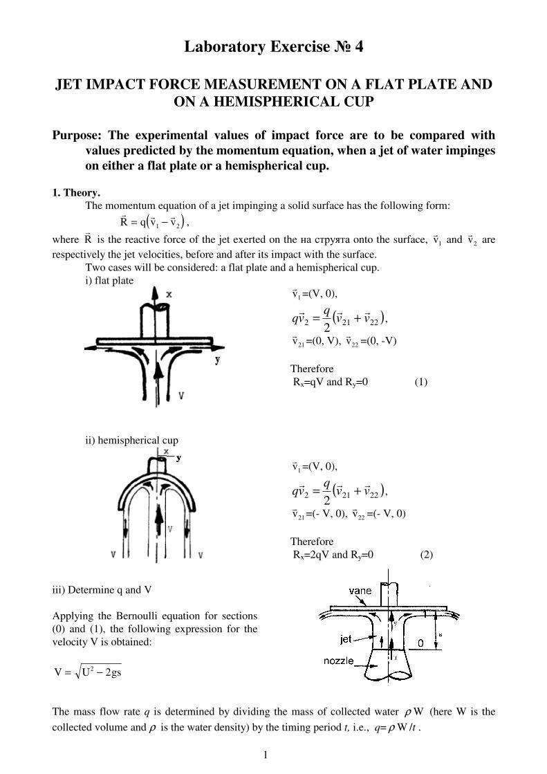
Laboratory Exercise № 4
JET IMPACT FORCE MEASUREMENT ON A FLAT PLATE AND
ON A HEMISPHERICAL CUP
Purpose: The experimental values of impact force are to be compared with
values predicted by the momentum equation, when a jet of water impinges
on either a flat plate or a hemispherical cup.
1. Theory.
The momentum equation of a jet impinging a solid surface has the following form:
( )r r rR q v v= −1 2 ,
where rR is the reactive force of the jet exerted on the на струята onto the surface,
rv1 and
rv2 are
respectively the jet velocities, before and after its impact with the surface.
Two cases will be considered: a flat plate and a hemispherical cup.
i) flat plate
rv1 =(V, 0),
( )222122
vvq
vqrrr
+= ,
rv21 =(0, V),
rv22 =(0, -V)
Therefore
Rx=qV and Ry=0 (1)
ii) hemispherical cup
rv1 =(V, 0),
( )222122
vvq
vqrrr
+= ,
rv21 =(- V, 0),
rv22 =(- V, 0)
Therefore
Rx=2qV and Ry=0 (2)
iii) Determine q and V
Applying the Bernoulli equation for sections
(0) and (1), the following expression for the
velocity V is obtained:
V U gs= −2 2
The mass flow rate q is determined by dividing the mass of collected water ρ W (here W is the
collected volume and ρ is the water density) by the timing period t, i.e., q= ρ W /t .

2
The volume flow rate is Q=q/ρ.
The velocity of water leaving the nozzle is U=Q/A, where А is the nozzle area.
iv) determination of the experimental impact force
T – spring force when the beam is horizontal
F – experimental impact force of the water jet on the vane
M – mass of beam assembly (excluding jockey)
m – mass of the jockey weight
• If no impact force, F = 0, the jockey is positioned at zero location on the scale and the
beam is horizontal. Then the moment about the pivot is:
Mg mg Tl l l1 2 3 0+ − = (3)
• If impact force is acting, F ≠ 0, the jockey weight is at x location on the scale and make
the beam horizontal. Then the moment about the pivot is:
( ) 0321 =−−++ lFlTxlmglMg (4)
Subtracting equation (3) from (4): 0=− lFmgx and consequently:
Fmg
x=l
(5)
2. Experimental scheme

3
3. Experimental procedure:
(i) Check that the apparatus stands vertically and that, when the tally is correctly positioned, the
beam is horizontal.
(ii) Fit the flat plate to the beam.
(iii) Place the jockey weight on the zero of the scale and set the beam horizontal by adjusting the
nut.
(iv) Close the supply valve and start the pump.
(v) Open the supply valve to achieve a layer of water on top of the flat plate.
(vi) Open fully the supply valve and set the beam horizontal by adjusting the position of the jockey
weight.
(vii) Note the position of the jockey weight on the scale and choose convenient settings for eight
jockey weight positions, equally spaced, using the full available range of the scale.
(viii) Place the jockey weight on the first setting and set the beam horizontal by adjusting the supply
valve.
(ix) Record the jockey weight position and measure the volume flow rate by timing the period for
35 liters of water to flow through the apparatus.
(x) Repeat steps (viii) and (ix) for the eight jockey weight positions. For the lower flow rates, the
collected water volume may be reduced, provided that the timing period does not become less
than 60 sec.
(xi) Close the supply valve and replace the flat plate with the hemispherical cup.
(xii) Open the supply valve to give a moderate flow rate; keeping the beam horizontal, adjust the
orientation of the nozzle to give a symmetrical flow from the plate (if possible).
(xiii) Repeat steps (iii) and (vi) to (x).
(xiv) Close the supply valve and stop the pump.
(xv) Record: mass of the jockey weight; diameter of the nozzle; distance between the beam pivot
and the vane; vertical distance between the nozzle and the vane.
4. Experimental data: Density of water, ρ =1000 kg/m
3
Mass of the jockey weight, m=………..kg
Diameter of the nozzle, d=………..m
Distance between the beam pivot and the vane, l = ………m
Vertical distance between the nozzle and the vane, s = ………m
Nozzle area, А=………………m2
(i) Flat plate
Position of jockey weight,
x
Volume flow rate readings,
Q=W/t
(mm)
Volume of water, W
(l)
Collection time, t
(s)

4
(ii) Hemispherical cup
Position of jockey weight,
x
Volume flow rate readings,
Q=W/t
(mm)
Volume of water, W
(l)
Collection time, t
(s)
5. Result treatment
(i) Flat plate
Position of
jockey
weight, x,
(m)
Experimental
impact force
Fmg
x=l
,
(N)
Volume
flow rate,
Q=W/t
(m3/s)
Mass
flow rate,
q=ρW/t
(kg/s)
Velocity of
water leaving
nozzle,
U=Q/A
(m/s)
Velocity of
water
impacting
vane
V U gs= −2
2
(m/s)
qV
(N)
Rx=qV
(N)
(ii) Hemispherical cup
Position of
jockey
weight, x,
(m)
Experimental
impact force
Fmg
x=l
,
(N)
Volume
flow rate,
Q=W/t
(m3/s)
Mass
flow rate,
q=ρW/t
(kg/s)
Velocity of
water leaving
nozzle,
U=Q/A
(m/s)
Velocity of
water
impacting
vane
V U gs= −2
2
(m/s)
qV
(N)
Rx=2qV
(N)

5
6. Graphical representation of the results:
Plot on two different graphs the experimental impact force F, as well as the theoretical reactive
force Rx as a function of qV for both the flat plate and hemispherical cup cases. Find the slope
F/qV of both graphs.
7. Analysis
On the basis of the plotted graph, analyze the following:
• whether the graphs are linear;
• whether the graph do not pass through the origin of the coordinate system and point out the
reasons for that;
• whether the slopes of the graphs are smaller than the expected ones and point out the factors
responsible for that;
• what are the possible experimental errors and state their effect upon the obtained results.
F F
R x Rx
F lat p late qV H em ispherical cup qV

Laboratory Exercise № 5
MEASUREMENT OF THE CRITICAL VALUE OF THE
REYNOLDS NUMBER
Purpose: The different types of flow are to be demonstrated using the
apparatus of Reynolds and the critical Reynolds number is to be
determined
1. Theory:
A. Flow types:
A.1. Laminar – at low velocities, the fluid
particles move along straight lines.
A.2. Unstable or transitional
A.3 Turbulent – at high velocities, the
fluid particles move in an irregular,
chaotic manner, which leads to their full
mixing.
B. Critical Reynolds number:
Re =Vd
ν, for circular pipes, d – pipe diameter, V – mean velocity, V
Q
d=
42
π ., ν -
kinematic viscosity coefficient
Recr – corresponds to the transition from laminar to turbulent flow, i.e., when the flow is
unstable, wavy:
ν
dVcr
cr
.Re = , where
2.
4
d
QV cr
crπ
=
The experiments are performed at normal engineering conditions that occur at some
disturbances and then: 4000Re2000 ≤≤ cr . The lower bound is usually taken as a
theoretical value of Recr: (Recr)theor = 2000.

2. Experimental scheme: Apparatus of Reynolds – Osborne Reynolds (1842–1912), Professor of Engineering
at Manchester University.
.
d =0.022m 1
4 3
5 2
2 7
6 entrance
exit exit
1- reservoir filled with a dye
2 - valve
3 - overflow
4 – reservoir filled with water
5 – transparent pipe
6 - rotameter
7 - needle
3. Experimental data:
t 0
water = ............. С0
ν water(t 0) = ........... using reference data
Q V
Q
d=
42
π . Re
.=
V d
ν
Flow type
m.l/s m3/s m/s
4. Analysis of the experimental data: а) Determine Recr.
b) Explain the nature of disturbances during the experiment.
c) Determine the relative discrepancy between the experimental and theoretical
value of Recr. What are the reasons for it?
d) Draw schematically the flow observations correspondent to each measurement.