Laboratory Study of Electromagnetic Initiation of Slip

T.Chelidze, N. Varamashvili, M. Devidze, Z. Tchelidze, V. Chikhladze

Introduction

In the experiments, initially aimed to finding resisitivity precursors of strongearthquakes in the upper layers of Earth crust by MHD-sounding an unexpected effectof microseismicity activation has been discovered (Tarasov et al, 1999). Theactivation of acoustic emission by electromagnetic field has been also observed inlaboratory experiments (G. Sobolev et al, 2000). In the first 6-month report we notedthat the field of MHD-dipole is quite small at distances of order of 100 km, where theeffect has been observed: for resistivity of rocks of order of 100-1000 ohmm (this isthe resisitivity of rocks at the depth 5-10 km in the test area, according to Tarasov etal (1999) at the distance of order of 100 km from the dipole source (this is thedistance to the area where the activation of microseismicity has been noted) theintensity of dipole field for the experimental source is of order of 10-5-10-6 V/m. Thesecond peculiarity of activation effect was that it occurs with 2-4 day delay after EMimpact; that means that the velocity of impact propagation is of order of 30 km/day =0.35 m/s.

Thus it is necessary to find at least phenomenological physical modelexplaining these two important details: long-range action and delayed response.

Phenomenological approach

Several possible mechanisms can result in the triggering effect of weakelectric field.

First of all, only the system, which is close enough to the critical state, canmanifest anomalous sensitivity to small external impacts. According to recentinvestigations, Earth’s crust in seismically active regions can be in the critical state orin the state of self-organized criticality (Bak et al, 1988; Scholtz, 1990). This canexplain the known phenomenon of seismic activation at filling large reservoirs, whichadd an insignificant contribution to existing tectonic strains. Another examples areseismicity activation by pumping of water in the boreholes (Sibson, 1994) and remoteaftershocks of Landers earthquake. According to King et al (1994) aftershocksregistered very far from the epicenter of the earthquake were generated by only one-half bar increment in stress, provided by the mainshock.

One of possible mechanisms can be the direct dielectric breakdown of rocksdriven by tectonic stress to the critical state. That means that the EM pulse should bestrong enough which is probable only in the source near-zone. In the far-field zone thepulse should be somehow amplified in order to cause dielectric breakdown (DB).Dielectric breakdown as a rule is accompanied by emission of elastic waves. Thisclass of models, which can be related as “underground thunderstorms” was advancedby A. Vorob’yov. The amplification can be realized in following ways:

i. Amplification of EM field by wedge-type inclusions.Local electric field of inclusion with conductivity g2, much larger then

conductivity of embedding media g1 can exceed the intensity of mean macroscopicfield. The largest effect is expected for the needle- or lens-shaped inclusions. It is wellknown that elongated conductive impurities in transformer oil enhance dielectricbreakdown. As the cracks in rocks are usually saturated with conducting pore fluid

and have form of lens or needle, some amplification of the applied field can beexpected: theoretically at the tip of the needle local field intensity is infinitely high.For very crude assessment we can use the expression for local electric field El at thedistance r from the tip of the conductive wedge (E. Kharitonov, 1983):

El = E0 (r/d)-v (1)

where E0 is the (uniform) field far from inclusion and d is some characteristicdistance. From experimental data is found that v ≈ ½. If we exclude the singular pointr = 0 and assume that d is, say, 10 m, then according to formula at r = 0.1 m from thecrack tip E ≈ 10E0 and for r = 0.001m E ≈ 100E0 .In order to assess the effect more precisely, some experiments were performed onphysical (two dimensional) model. The aluminum “double wedge” inclusion has beenglued on the bottom of flat glass vessel (Fig. 1) which was filled with tap water.Specific resistivities of metal and fluid were 2.810-8 ohmm and 100 ohmmcorrespondingly, i.e. the resistivity ratio was 1010. The voltage 20 V has been appliedto electrodes, separated by 38 cm; the uniform potential gradient is thus 0,526 V/cm.Electrical potential U has been measured along seven profiles (Pr 1-7) oriented bothalong and across the large axis of elongated inclusion (see Fig.1). On the Fig.2 areshown the equipotential lines (dots) and current lines (full lines). The significantconcentration of equipotential lines at the tips is evident. Fig. 3 shows potential valuesmeasured along profiles 1-1, 2-2 and 3-3.

Fig. 4 shows U and E variations along profiles 4-4, 5-5 and 7-7 and Fig. 5shows E along profiles 1-1, 2-2 and 3-3.

Thus at the tip of the crack the local field can be orders of magnitude largerthan the mean macroscopic field (Fig.5); that can give amplification of intensitry fromµV to mV which still is not enough to cause dielectric breakdown.

ii. Amplification of EM field in the random lattice model.Besides above discussed «wedge» model there is another class of models which alsoexplain local amplification of applied voltage, namely, percolation (random lattice)models. It has been shown (Archangelis et al, 1986; Benguigi, 1988) that distributionof voltages on the random lattice of resistors and insulators is multifractal and at thepercolation threshold pc the maximal voltage drop Vmax occurs on singly connected(so called red) bonds which carry the total current passing through the network. Thereare two models of electrical breakdown of the random lattice, dielectric and fuse. Inthe first model the system is conductor-loaded insulator. An insulating elementbecame conducting (breaks) at the voltage higher than Vth. Than the whole systembecame conducting at the breakdown voltage Vb which strongly depends on theconcrntration of conducting bonds p.In the second (fuse) model the system isinsulator-loaded conductor. Here the conducting element is fused , i.e. becameinsulator, if the current, flowing through it is larger than threshold current Jth. Again ,the whole system fuse (became insulator) at carrying the current Jb which srtonglydepend on the concentration of conductors p.Near percolation threshold pc when the infinite cluster of conducting bonds spans thewhole system, the breakdown voltage Vb has a typical power law form (Archangeliset al, 1986; Benguigi, 1988):

Vb = (p-pc)ν (2)

and goes to zero as p→p? . Here ν is the exponent of correlation length ξ. For two-dimensional systems ν = 4/3. According to (2) at p→p? the system breakdownvoltage became very low.

The geological formations can be considered as mosaics of insulating(minerals) and conducting (brine-saturated pores and cracks), which in some areas areclose to percolation threshold. This in principle can explain the local breakdownphenomenon.

It should be noted that it is difficult to explain the time lag (2-3 days)between MHD impact and activation of microseismicity in any of above local voltageamplification models as the electric field propagates with high velocity.

iii. Seismohydraulic mechanism of activation of seismicity.We’ve noted that in order to initiate fracturing by EM pulses the system should beclose to the critical state, in our case close to the state of mechanical instability. Thecritical shear stress on the fault τc is:

τc= c+µ(σn – Pf) (3)

where c is resistance to fault displacement due to its partial cementation, µ is frictioncoefficient, σn is the stress component, normal to the fault plane , Pf is fluid porepressure. It is evident, that in order to provoke mechanical instability, EN pulseshould affect at least one of parameters of above formula in order to change τc. Itseems that µ ,σn and Pf can be affected by EM pulse. For example, due topiezoelectric effect µ and σn can be favorably changed. The weakening of faultsunder EM impact can also be connected with interaction of pore fluid and mineralbackbone, namely:

a. application of EM pulse can drive pore fluid into the “dry” cracks. Thisdecreases surface fracture energy, which means either enhancement of crack growthby Griffith’s model of fracture or just decrement of friction coefficient µ.

b. electrical impact can provoce electrokinetic flow in the porous rock(electroosmosis) and thus increase pore pressure Pf .c. strong EM impact can generate so called electrohydrodynamic effect (EHD)which has been discovered in fifties (Nesvetailov, Serebryakov, 1966). EHD effectmeans that water saturated porous solid can be destroyed by strong enough EMpulses and this has found industrial applications. The mechanism of EHD effect isnot known exactly. The most popular explanation is cavitation or generation of smallgas bubbles by applied EM pulse; their collapse generates in the fluid transient stressfields, which destroys a solid.

First two mechanisms in principle can explain the considerable time lagbetween impact and (remote) respond as the pore fluid migration or diffusion underelectric field is relatively slow process.

Rigorous quantitative approach to above mechanisms is very difficult as allthese models contain some parameters which can not be measured exactly, say,closeness to the percolation threshold of geological formation at the depth 5-10 km,water content, stress state, etc. Thus at the moment the most important is to prove thepotential of EM pulses to trigger mechanical instability in laboratory experiments andcreate reasonable physical models of phenomenon.

Experimental set up.

The experimental set up has been designed in such manner that the mechanical systemcould be easily driven to the critical state where the triggering of mechanicalinstability by some weak impact such as electrical pulse became more probable. Thesystem consists of two pieces of rock; the upper piece can slip on the fixed supportingsample if the latter one is tilted up to the critical angle.The set up can be used for experiments in various conditions, “dry” and “wet”. In thelatter case the sample holder can be immersed in the bath with water.The general view of the set up is shown on the Fig. 6.i. Mechanical part.The device brings the mechanical system (two pieces of rock, one of which can slipon the supporting sample) to the critical state, that is, to the critical slope of thesupport. The regulation and fixing of the tilt is realized by means of vernier systemwith an accuracy 15'.The second important detail is the acoustic emission sensor, which responds toelementary slip events of upper sample on the supporting one. It is the relatively lowfrequency sensor (25-100 KHz). The sensor was applied to the frame of the device orto the supporting (fixed) rock sample using salol.ii. Electrical part.Electrical part consists of EM pulse generator and acoustic signals amplifier. Forexperiments it was necessary to assemble a system, generating high intensity AC andDC fields. For this a high voltage linear amplifier has been built. The principalscheme of linear amplifier (of class “A”) is given on the Fig.7. It has two outputs, forAC and DC voltages. The signal from the standard generator with amplitude 0.5-5 Vis applied to the input of the amplifier and goes out from the output with amplitude upto 1300 V. The high voltage pulses are applied to electrodes, placed under thesupporting rock sample. The electrodes are of various forms (Fig. 8) and can beconnected in various combinations. Other configurations of electrodes will be tested.Another amplifier was designed for registration of acoustic signals from the sensorswhich respond to the slip events. This is a two-channel low-noise amplifier (Fig.9);the amplification rate of channels can be regulated separately. The amplifier’s outputvoltage is sufficient for registration of acoustic signals by the sound card of PC. In thescheme the output clipper is installed which defends PC input from voltage overloadand indicates overload of low-noise amplifier as well. The PC used was Pentium II.The scanning of the process was performed on the frequency 96 kHz, i.e. samplingrate was 1/96 000 s.

ii. SamplesThe supporting and the sipping blocks were prepared from glass, basalt, marble andgranite. They were coarsely finished after sewing.

Experimental results

i. The critical angle measurementsThe critical slopes of slip for various couples of rocks were defined. For each

sample 20 measurements of critical angle have been made. The results are shown inthe Table 1. and Fig.10. For all samples, except basalt the critical angle was in therange 8-13o ; for basalt it was higher – 25 o. The data are scattered around these meanvalues with standard deviation of order of 0.5o. The experiment on glass discs showsthat the diameter and thickness of samples do not change the critical angle notably.

As the critical angle depends on many parameters which can change in time(humidity and temperature, surface roughness, friction coefficient), its value has beenalways controlled before experiments with EM pulse.

Table1.

Runs 1 2 3 4 5 6

1 9,3 11,3 12,3 12 25,3 9,12 8 10,3 13 12,3 26,3 8,33 9 11,3 12,3 12,3 25,3 104 8,24 11 13,1 13 24 8,35 9,3 11 11,3 13,5 25,3 8,16 9,4 10,3 10,3 12,3 26,3 10,27 8 11 11 12 25,3 10,38 8,16 11,3 10,3 12,3 26 10,39 8,2 10,3 11,3 13 25,3 8,310 8 10 13 13,3 26 8,111 8 9,3 11 12,3 26 8,3212 8 9,34 11,3 11 26 8,413 9 10 12 10,1 25,4 1014 8,3 10,3 11 12,3 24,2 1015 9,12 11 11,3 11 24 9,316 8,2 10,3 12,1 12,02 23,3 917 8 9,3 12,12 12 24,3 8,418 8,3 9,3 11 13 26 9,1219 9 10 11,3 12,02 24,1 1020 9,2 10,3 11 13,3 25,3 9,3

Average 8,536 10,347 11,601 12,252 25,185 9,142st.dev 0,54443 0,692342 0,841689 0,843262 0,895177 0,802917Variance 0,296404 0,479337 0,70844 0,711091 0,801342 0,678606

ii. Assessment of friction coefficientFrom the elementary physics it is known that the friction coefficient µ for the

body placed on the inclined plane can be calculated from the condition that at thecritical angle αc, when the body slips down the plane, the friction force F equals zero:

0)( =−= cc SinCosmgF ααµ

where m is the mass of the upper (slipping ) sample, g is gravity force acceleration,or

µ = tgαc

Using data on the critical angle, obtained on the tested materials (Table 1) theaverage values of fracture coefficient for finished samples are varying from 0.14 to0.23 and for the saw-cut basalt sample µ = 0.47.iii. Laboratory modelling of EM-quakes (experimental procedure and case stories)

The main objective of experiments was to find out whether EM-pulse canindeed displace the rock sample, placed on the supporting (fixed) sample at the slopeof support, less than but close to the critical slip angle.

Surprisingly, all tested samples were eventually displaced (slipped) by strong EM-pulses. The amplitude of DC-pulses was 1200 V, duration from 5 to 10 s, and intervalbetween pulses was also from 5 to 10 s. In the following experiments the negativepole of generator was applied to electrodes a and b, and the positive one to theelectrodes c and d (Fig. 8).

After finding critical angle the slope of support was decreased by 2-3o. In thisstate the upper sample was not moving for many hours (days), which means that othersources of instability such as building vibration by trucks, elevator, wind, etc are notstrong enough to initiate the slip. As the critical angle for the rough surface is varying(it is impossible to reproduce exactly the arrangement of asperities between supportand slipping block) the sample was kept for at the angle α<αc for 10 minutes and onlyafter this exposition time subjected to EM-impact. That allows assessing correctly thestatistics of EM-activation, as the probability of slip in time intervals without EM-impact can be compared with that in time intervals covering the whole EM-activationperiod (including gaps between pulses). Actually the probability of slip without EM-impact at α<αc was zero: no slip was observed during 10 min. repose period.Application of EM-pulse initiates slip either during pulse (i.e. in the active phase),either after it (i.e., in the passive phase) or after application of several pulses. Quiteoften the slip was being initiated in the passive phase, after switching off the pulse.

The case histories of slip are as following:i. basalt sample (test1) has been displaced soon after application of the

pulse, in the active phase (Fig.11). The acoustic sensor was applied tothe supporting sample. Here and in following tests the upper traceshows acoustic sensor’s output and the lower one records the switchingon and off of the EM-pulse (the thick lower trace corresponds to theactive phase, i.e. current on)

ii. Fig 12 presents the history of the test 2 on the same sample of basalt;here the sensor was applied to the lower side of the organic glass frameunder the supporting sample.

iii. Fig. 13 shows in more detail the initial stage of slip in the test 3 on thesame basalt sample. Fig. 14 and 15 present the recordings of microslipevents, which happen both in the active and passive phases. In the test3 the sensor was applied to the upper part of the organic glass frame.

iv. Fig. 16 presents the results of labradorite sample testing. The EM-induced slip has been observed soon after the application of pulseduring the active phase. On the Fig. 17 the stretched initial stage isshown. Fig. 18 shows the recordings of microslip events.

It seems that in many cases the slip occurs after switching off the pulse. It isevident also that finished samples are displaced more easily. It is interesting that someweak acoustic pulses were recorded before final slip, which means that before finalsliding some microslips are also induced by application of EM-pulses.

iii. Assessment of electrical field intensity (EFI) on the slip surface.In the following experiments only basalt sample was studied.The voltage applied to the samples was 1200V; nevertheless it is important to

know the electrical field, acting on the slip surface.The calculation of electrical field on the slip surface can be carried out using

standard equations of electrostatics.For the pair of co-planar electrode system used in our experiment the EFI on

the distance 2.5 cm (i.e. z = 2.5 cm) from the electrodes under voltage 1250 V varies

from approximately 10 V/cm and 40 V/cm if the space is filled by material withdielectric constant 5 (characteristic for basalt in room conditions).

The calculated values are characteristic for homogeneous media. Real samplesare very heterogeneous; that means that the EFI should also be measuredexperimentally. EFI on the outer side of interface between supporting and slidingsamples has been measured by digital multimeter with accuracy ± 0.01 V. The voltagewas measured relative to the negative pole. The distribution of EFI prove to be rathermosaic: the values of V along the outer perimeter of slip surface vary from 0.01 to 57V and the average value is around 8 V.

These values are in accordance with above theoretical assessment.We can conclude that electrical impact of order of several volts can induce slip

in the system close to the critical state.iv. Assessment of mechanical equivalent of electrical impactFor assessment of mechanical equivalent of electrical impact both direct and

theoretical methods were used.In the first case the mechanical force, initiating slip at the same angle α<αc

that has been set in experiments with EM-impact, was measured by spring (accuracy± 0.01N) and by torsion (accuracy ± 0.005 N) dynamometers. Both methods givecomparable results. The force, equivalent to slip-initiating EM-impact is of order of0.2 N.

Another way to get mechanical equivalent is to calculate it from the generalequation of balance of forces for a sample placed on the inclined plane:

)( ααµ SinCosmgF −=As far as µ is known ( µ = 0.47) slip-initiating force can be calculated for any

angle (Fig. ). For example if αc equals 25o , at α = 24o50′ the initiating force is of0.42 N. This value is of the same order as in direct experiments (0.2 N).

Thus in situation close to the critical one even 0.02 N force can initiate slip ofthe sample, weighting 700 g.

v. Statistics of EM-slipsIt is well known that surface phenomena are rather complicated and are prone

to influence of many factors: surface roughness, configuration of asperities, humidity,temperature, chemistry of contacting materials, etc.

So it is quite natural that in case of contact of rough enough surfaces onlysmall part of EM-pulses initiate motion, namely the pulses that are applied at the mostfavourable arrangement of asperities on the slip surface.

A general idea on the efficiency of impact can give the results of one series ofexperiment on the basalt sample. The total probability of EM-initiation P is7/94=0.07, the probability of slip during the pulse is 0.04 and that of slip afterswitching off the power is 0.3.

The probabilities of initiation for various stages of impact for are: during firstpulse – no case; after first pulse – 0.01; during second pulse – 0.02; after second pulse–0.01; during third pulse – 0.02, etc. Of course, these probabilities vary from oneseries to another one but the total probability is not changing considerably.

It should be noted that the observed process is extremely complicated and itsmechanism is not clear. Nevertheless, the experiments show that EM-initiation of slipin mechanical system that is close to the critical state is quite real.

vi. Probable physical mechanismIn order to understand physics of EM-slip it is necessary to consider

fundamentals of surface phenomena. Intermolecular and intersurface forces,

responsible for adhesion and friction, can be loosely divided into three categories: i.purely electrostatic, arising from the Coulomb interaction between charges; ii.polarization forces arising from the dipole moments, induced by internal (boundcharges, dipoles) or external electric field; iii. quantum-mechanical forces, responsiblefor covalent bonding and steric interactions. All these forces can act simultaneously,resulting in some total adhesion (friction) force. For friction we have:

` Ff = µ Fn

where µ is friction coefficient and Fn is the normal component of force acting on thebody (gravity, compression).

From above classification it can be deduced that in principle external electricalfield can affect the intersurface adhesion (friction) forces, changing µ and thusinitiating slip of the body, placed on the inclined plane. EM-impact can affect alsoFn of the body containing piezoelectric materials.

As far as the EM-activation is clearly observed on samples, that are practicallyfree of piezoelectric minerals (basalt) we exclude piezoelectric effect as a principalmechanism of EM-slip.

Having in mind that quite often initiation of slip was observed after switchingoff the power, it seems reasonable to accept the hypothesis that the applied EM-pulseaffects the electrostatic and/or polarization component of the intersurface adhesiveforces.

On the dynamics of inter event time interval distribution of earthquakesaround IVTAN polygon

Sequences of time intervals in seconds between all consecutive earthquakes (time gapsequences) around IVTAN polygon in 1975 –1996 were analyzed using standard toolsof nonlinear dynamics (Abarbanel et al., 1993).

Sequences of time gaps of different time periods were considered. Namely,time period before beginning of experiment (1975-1983), time period of cold and hotruns 1983-1988, and time period after experiment (1988-1992) as well as time periodlong after the cessation of experiment (1992-1996). Considered time intervalsequences are approximately of equal length (about 3660). In Fig.1 results ofqualitative analysis of mentioned time series by Iterated Functions System (IFS)Clumpiness test are presented. It is evident that the time intervals betweenearthquakes manifests some nonlinear structure after beginning of EM-impacts(Fig.1b). For comparison the test results for the Lorentz attractor are shown on Fig.1e. Before EM experiments (Fig.1a) and after it (Figs. 1c, 1d) the test does not revealclear structure.

The IFS Clumsiness test is a qualitative method. In order to get quantitativemeasure of nonlinear structure in this time series the correlation dimension d2 hasbeen calculated. Correlation dimensions vs. embedding dimension of these time seriesare presented in Fig. 2.

As follows from our analysis, after beginning of experiment correlationdimension of time interval sequence decreases to the level, characteristic for lowdimensional processes (Fig. 2) i.e. events of corresponding time series become muchmore interdependent (almost at the same rate as the Lorentz process). At the sametime according to the results of qualitative IFS analysis (Fig. 1b) process cannot beregarded as deterministically chaotic. On the other hand after termination of

experiment considered dynamics become more randomized both qualitatively (Fig.2.c, d) and quantitatively: correlation dimension exceeds low dimensionalitythreshold -5).

Fig.3 represents time series correlation dimension variations vs. embeddingdimension for long integral time. The conclusion is that the long time series coveringthe whole catalog manifests a low correlation dimension due to the strong lowdimensional contribution of experiment period (triangles). The influence of lowdimensional period is still stronger for shorter time series, containing equal (3600)time intervals before and after the experiment period (squares).

The similar analysis, carried out for time series of magnitudes, does not revealany significant differences between experimental period and background seismicprocess.

The uncovered regularity seems very interesting as it testifies possibility ofchanging seismic regime of the test region by relatively weak EM-impacts. Thispreliminary result should be tested very carefully using various surrogate tests(randomized sequences).

Fig. 1. IFS-clumpiness test for inter-event time interval sequences, a) 3600 inter-event time intervals before beginning of experiment (1975-1983). b) 3600 inter-eventtime intervals after beginning of experiments (1983-1988), c) 3600 inter-event timeintervals immediately after accomplishing of experiments (1988-1992), d) 3600 inter-event time intervals long after accomplishing of experiments (1992-1996), e) Lorentzprocess.

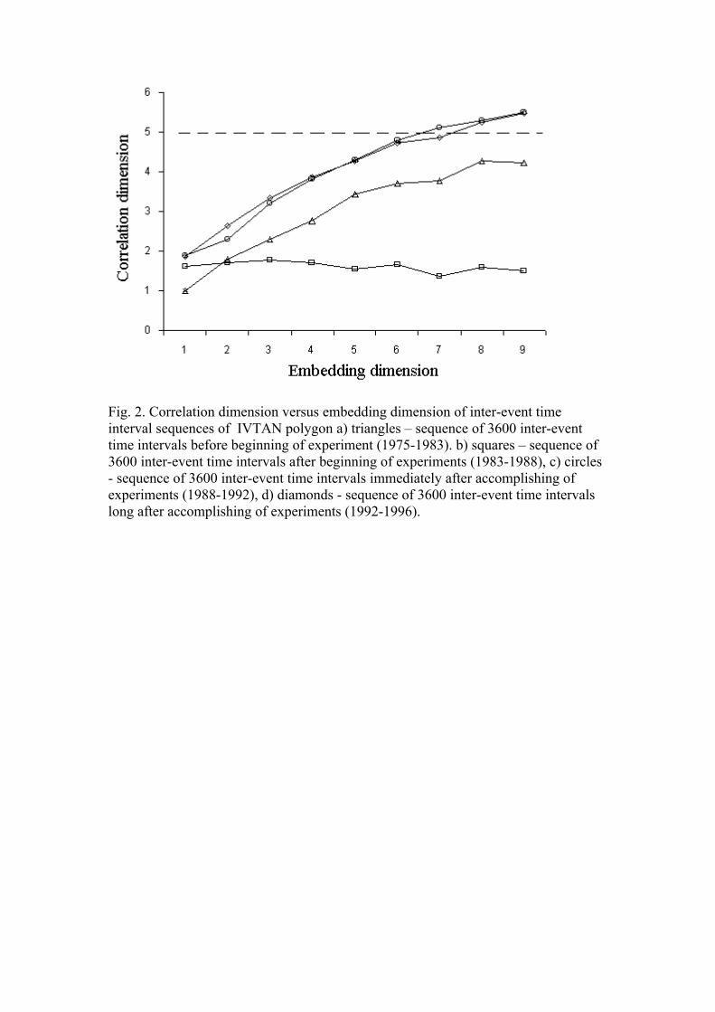
Fig. 2. Correlation dimension versus embedding dimension of inter-event timeinterval sequences of IVTAN polygon a) triangles – sequence of 3600 inter-eventtime intervals before beginning of experiment (1975-1983). b) squares – sequence of3600 inter-event time intervals after beginning of experiments (1983-1988), c) circles- sequence of 3600 inter-event time intervals immediately after accomplishing ofexperiments (1988-1992), d) diamonds - sequence of 3600 inter-event time intervalslong after accomplishing of experiments (1992-1996).

Fig. 3. Correlation dimension versus embedding dimension of inter-event timeinterval sequences for long integral time series: a) triangles - integral time series forthe whole period of observation (1975-1996), b) squares – integral (jointed) timeseries consisting of two equal length (3660 time intervals) parts from 1975 to1988,both before and after beginning of experiments. c) circles – random numberssequence, d) asterisks – Lorenz time series.

Conclusions

The phenomenological analysis of possible physical mechanisms of MHD-induced microseismicity has been done.

The experimental device for measuring local electric field of the crack-likeconducting inclusion in the less conducting medium has been assembled. Experimentsshow that close to the tips of inclusion the electric field is amplified by several ordersof magnitude. In the percolation state the voltage can be amplified

The experimental set up for laboratory modeling of impact of electromagnetic(EM) pulses on the stability of mechanical system, which is close to the critical statehas been built. The critical angle of slip without EM-impact has been measured.

The preliminary experiments, carried out in dry environment, show that strongEM-pulse (1200 V) induces acoustic emission and eventually, sliding of a sample ofrock (granite, basalt, labradorite), placed on the supporting sample, which is inclinedat the slope, close to, but less than the critical angle.

The mechanical equivalent of electrical force, initiating slip has beenevaluated both theoretically and experimentally: it was of order of 0.20 N for theslope of support, used in experiment.

Statistics of EM-slips has been studied: the probability of EM-activation byseries of pulses was found to be of order of 0.07.

Analysis of sequences of time intervals in seconds between all consecutiveearthquakes (time gaps) around IVTAN polygon in 1975 –1996 using standard toolsof nonlinear dynamics shows surprising result: during the EM-impact period thecorrelation dimension of time gap sequences is of order of 1.5 that is close to Lorentz

process’ dimension; before and after experiment period gap times manifest highcorrelation dimension, close to 5. This can signify that EM-impacts introduce someorder in time gap distribution. Time series of magnitudes do not show any significantdifference in nonlinear structure characteristics.

These preliminary results allow putting forward the hypothesis that EM-pulsessomehow control the time gap sequence that is we have an analogue of controllingdeterministic chaos. In our case we suppose that EM-impacts control nonlinear lowdimensional structure of time gaps.

Figures

Fig. 10. The values of critical angles of slip for following pairs of materials:Stars – basalt; diamonds – glass (diameter 2 cm, thickness 10 mm); quadrangles –glass (diameter 7.5 cm, thickness 10 mm); triangles – glass (diameter 9.5 cm,thickness 15 mm); crosses –glass (diameter 14 cm, thickness 12 mm); circles –labradorite.

Fig. Theoretical dependence of slip-initiating mechanical force on supportingplane inclination angle α.

0100200300400500600700

20 21 22 23 24 25 26

angle,degrees

forc

e, g

Series1

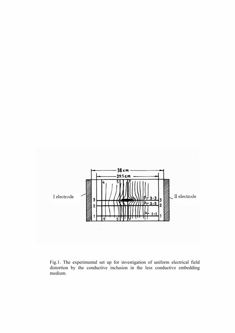
Fig.1. The experimental set up for investigation of uniform electrical fielddistortion by the conductive inclusion in the less conductive embeddingmedium.

Fig. 2. Equipotential lines (dots) and current lines (full lines) aroundconductive inclusion.

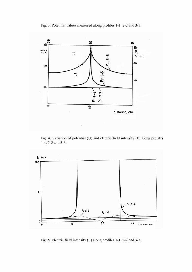
Fig. 3. Potential values measured along profiles 1-1, 2-2 and 3-3.

Fig. 4. Variation of potential (U) and electric field intensity (E) along profiles4-4, 5-5 and 3-3.

Fig. 5. Electric field intensity (E) along profiles 1-1, 2-2 and 3-3.

Fig. 6a. The mechanical part of the set up: 1- supporting sample; 2 – slidingsample, 3 – slope regulating unit; 4 – acoustic sensors; 9 – sponge for shockadsorption.

Fig. 6b. The full view of set up: 5 – electric DC-pulse source with linearamplifier; 6 – two-channel amplifier; 7 – computer for recording acousticemission on the audio-card of PC; 8 – pulse generator with variable frequency.

Fig.7. The principal scheme of linear amplifier.

Fig. 8. The configuration of electrodes, located under the supporting sample.

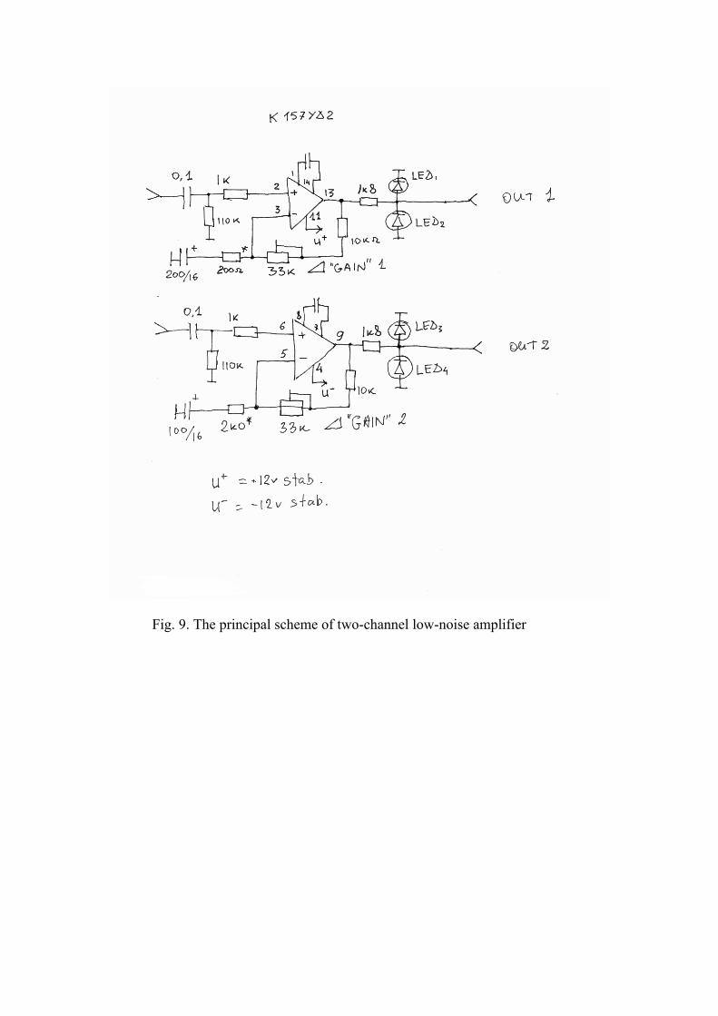
Fig. 9. The principal scheme of two-channel low-noise amplifier

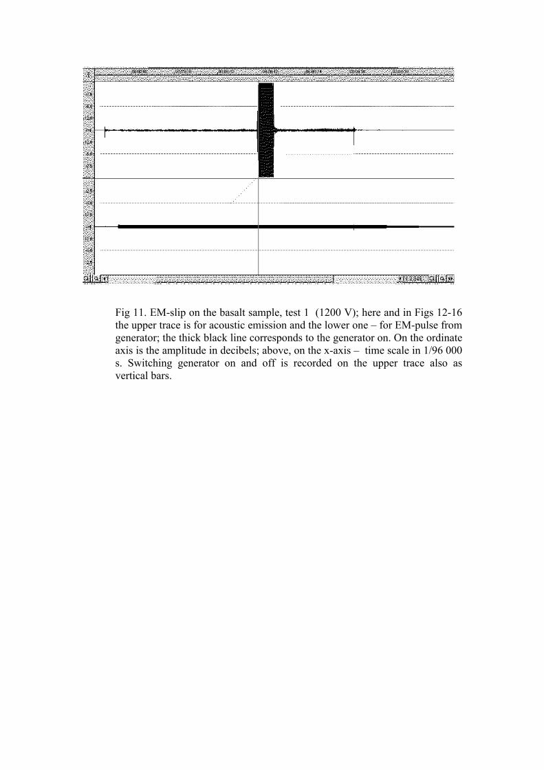
Fig 11. EM-slip on the basalt sample, test 1 (1200 V); here and in Figs 12-16the upper trace is for acoustic emission and the lower one – for EM-pulse fromgenerator; the thick black line corresponds to the generator on. On the ordinateaxis is the amplitude in decibels; above, on the x-axis – time scale in 1/96 000s. Switching generator on and off is recorded on the upper trace also asvertical bars.

Fig. 12. EM-slip on the basalt sample, test 2 (1200 V).

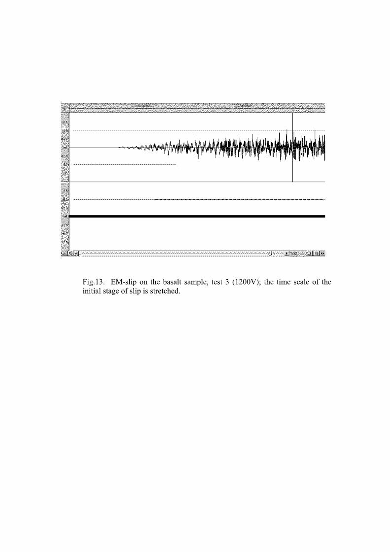
Fig.13. EM-slip on the basalt sample, test 3 (1200V); the time scale of theinitial stage of slip is stretched.

Fig. 14. EM-slip on the basalt sample, test 3 (1200 V); recordings of microslipevents.

Fig. 15. EM-slip on the basalt sample, test 3 (1200 V); recordings of microslipevents.

Fig. 16. EM-slip of the labradorite sample, test 4 (1200 V); slip happens in theactive phase.

Fig. 17. Fig. 16. EM-slip of the labradorite sample, test 4 (1200 V); sliphappens in the active phase. The initial stage of the slip is stretched.

Fig. 18. Fig. 16. EM-slip of the labradorite sample, test 4 (1200 V); microslipevent which happens in the passive phase is shown.

ReferencesH. Abarbanel, R. Brown, I. Sidorovich, R. Tsimring.1993. The Analysis ofObserved Chaotic Data in Ophysical Systems. Rev. Mod. Phys. 65, 1331-1392.L. de Archangelis, S. Redner and A. Coniglio. 1986. Multiscaling approach inrandom resistor and random superconducting networks. Phys. Rev., 34,45656-4673.P. Bak, C. Tang and K. Wiesenfeld. 1988. Self-organized criticality. Phys.Rev., A38, 364-374L. Benguigi. 1988. Simulation of dielectric failure by means ofresistor-dioderandom lattices. Phys. Rev, B 38, 7211-7214.E. Kharitonov. 1983. Dielectric materials with heterogeneous structure.Moscow, Radio and Communication (in Russian).G. King, R. Stein et al. 1994. Static stress changes and the triggering ofearthquakes. Bull. Seism.Soc. Am. 84, 935-953.G. Nesvetailov, E. Serebriakov. 1966. Theory and practice of electrohydrauliceffect. Minsk (in Russian).C. Scholz. 1990. The mechanics of earthqakes and faulting. Cambridge Univ.Press. Cambridge.R. Sibson. 1994. Crustal stress, faulting and fluid flow. In: Parnell J (Ed),Geofluids: Orugin, Migration and Evolution of Fluids in Sedimentary Basins.The Geological Soc. London, pp. 69-84.G. Sobolev, A. Ponomarev, A.Avagimov, V. Zeigarnik. 2000. Initiatingacoustic emission with electric actions. Report on ESC conference,N. Tarasov, H. Tarasova, A. Avagimov and V. Zeigarnik. 1999. The effect ofhigh-power electromagnetic pulses on the seismicity of Central Asia andKazakhstan. Volcanology and Seismology (Moscow), N4-5, 152-160 (inRussian).