labour market and price behaviour in jamaica · labour market and price behaviour in jamaica ......
TRANSCRIPT

1
Labour Market and Price Behaviour in Jamaica
Wayne Robinson Research Services Dept.
This version: November 1998

2
Labour Market and Price Behaviour in Jamaica
Introduction :
Conceptually, an inflationary episode is probably far easier to recognize than to precisely define.
As Frisch noted, the problem with inflation begins with the attempt to define it. Generally inflation has
been defined as a “process of continuing rising prices or equivalently falling value of money.”1 Inflation
is hereby characterized as some dynamic process involving sustained increases in the general price level.
This definition however has been cited as referring only to the symptoms of inflation. More specialized
definitions, focusing on the cause / effect relations, have taken either a structuralist, monetarist or a
hybrid perspective.
The structuralist approach identifies supply rigidities as the major cause of inflation. These
rigidities arise from differences in productivity, wage rates, price and industrial elasticities in the
`progressive’ and `static’ sectors which result in cost pressures. For an open economy therefore, “the
domestic rate of inflation results from imported inflation as well as from the differential between the rates
of productivity growth in the traded and non-traded goods sector.”2 The neo-structuralist goes further to
argue that there is a circular and inertial process of prices marked up over wages and wages indexed to
prices. Successive attempts to maintain or increase wages and profits are the main cause of inflation
and not money supply growth. Thus inflation is seen as a cost-push phenomenon.
The monetarist argues however that the structuralist approach does not adequately explain the
1Laidler (1975) pg 741.

3
transmission mechanism. Unless we assume a very flexible velocity of circulation of money, then a rise in
prices caused by wage or other cost increases with no offsetting increase in the money stock would
generate higher unemployment. To prevent this, the government will be forced to increase the money
supply. The monetarist approach sees inflation as being “determined in the money market and its pace
is set by the growth rate of money and the evolution of inflationary expectations which are the sole
determinants of velocity.”3 This however relies on the assumption of stable velocity. However if velocity
is unstable, then prices may increase without increases in the money supply simply because velocity is
increasing. The monetarists argue however that empirically velocity is by and large stable over time.
Inflation can thus characterized as demand-pull.
For our purposes we may tentatively define an inflationary process as the existence of dynamic
factors (monetary and/or non-monetary) which results in increases in nominal money income relative to
the value of available resources (output).
Adopting a strict monetary perspective, it has been argued that price increases in Jamaica have
been caused by excessive growth in the nominal money supply. The expansion in the nominal money
supply has had the effect of increasing effective demand in the context of declining productivity. Along
this line Thomas(1994) has argued that inflation is transmitted primarily through movements in the
exchange rate. Calvo(1994) has argued that the persistence of inflation is due to a combination of
factors such as the growth in the money supply, reserves accumulation (which fuels money supply
2 Frisch,(1983) pg175.
3P. Cagan , “The monetary dynamics of hyperinflation” in Studies in the Quantity Theory of Money. ed M. Friedman.

4
growth), exchange rate depreciations and excessive wage increases. Other economists, from a
structuralist position4, hold the view that the inflationary experience in Jamaica has been mainly due to
the structural imbalances that originated in the colonial era and which still persist today. Further, it has
been argued that rapid increases in production costs that are easily passed on to consumers are the main
source of inflation. This incidence of cost inflation has been attributed to increases in the price of
imported raw material and consumer goods along with exorbitant increases in the local wage bill due to
vigorous trade union activities.
The latter, though not new, have come into a sharper focus in the debate as there have been
recent concerns about the impact of significant wage increases, both in the private and public sectors, in
the past four years on inflation. The issue is of particular significance in the context of export led growth,
where low inflation is essential for external competitiveness. The pundits’ position has been echoed as
far back as the mid 1960s when Lewis(1964) noted “one of Jamaica’s principal problems today (and in
previous years) is that the costs of production are rising at such a rate that our competitive position in
the international markets is jeopardized. The reason for this is simple, incomes are rising more rapidly
than productivity. When this happens the entrepreneur has no alternative but to increase prices or
mechanize.”5
Alesina and Perotti (1995) have argued convincingly that the structure of the labour market and
the bargaining process is the major determinant of the effect of wages on prices. They conclude that an
economy that has one body that negotiates with employers on the behalf of workers will experience less
4See for example Latibeaudiere (1974)

5
inflationary pressure arising from the labour market. On the other hand, an economy which has a labour
market structure in which there are a number of competing negotiating institutions or more significantly,
few vibrant unions (oligopoly), will tend to have greater inflationary pressures arising from the labour
market.
Griffith(1976) argues however that unless trade unions’ power is constantly increasing,
oligopolistic labour markets will not generate inflation. He argues that “whether the labour market is
highly unionized or not may clearly affect the way in which inflation proceeds but is irrelevant as regards
to its cause.”6 The effect of the labour market on prices is determined primarily by the government’s
employment target and how it is achieved.
Recently, Whitter and Reid (1994) examined the relation between wages and inflation. Their
analysis provides a detailed account of the nature of the Jamaican labour market. Using cost and
demand approaches, they concluded that a 10.0 percent increase in total labour costs results in a 4.5 to
6.0 percent increase in prices. This conclusion however is based on highly restrictive assumptions that
there are no changes in labour productivity and consumption patterns. Also, they fail to recognize the lag
effects and the interrelations between the factors causing inflation. Generally, during high inflation
episodes it is difficult to confirm or reject particular models of the inflationary process as all nominal
variables move in the same direction, and there is generally some feedback mechanism.
In the context of recent concerns about labour market instability, this paper attempts an a
preliminary assessment of the impact of wage rates on inflation within the Jamaican economy. The paper
5Lewis (1964)

6
seeks to answer whether or not inflation originates in the labour market or in the money market. It
employs simple Granger causality tests and the Harberger’s test for demand vs wage pull inflation in a
cointegrated framework. The analysis begins with an overview of the trends in wage and price inflation.
This is followed by an attempt to quantify the relation between the two variables.
Wages, Prices & Productivity in Jamaica
When compared to the main trading partners, Jamaica can be considered as a high inflation
economy. This is particularly the case during the earlier part of the 1990s when the inflation rate
averaged 41.4 percent. During this time inflation amongst the trading partners averaged below 8.0
percent. Since 1980 the local annual inflation rates averaged 23.9 percent. One may argue that given
this present structure the long run inflation of the economy would lie somewhere around 20.0 percent.
A key feature in Jamaica’s inflation profile is the cyclical periods of high inflation followed by
steep contraction and some form of stabilization. (See Fig i) Two distinct periods of significant
inflationary episodes are of particular importance.
The first commenced in 1982/83. This episode lasted for about three years with the annual
point to point inflation rate moving from 6.97 percent in 1982 to 26.82 percent in 1984 and 23.35
percent in 1985. The largest shock occurred in 1983 where the rate moved from 6.97 percent to 20.67
percent. The greater part of the shock occurred in the last quarters of 1982 and 1983.In fact between
1982 and 1985 prices rose by an overall 88.8 percent. Price movements in this period maybe linked,
amongst other things, to oil price changes and exchange rate devaluations resulting from changes in the
6Griffiths (1976). Pg 60.

7
foreign exchange regime.
Some measure of stabilization was achieved over the following three years when the inflation
rate declined from 23.35 percent in 1985 to 8.55 percent in 1988. It must be noted that although single
digit inflation was achieved, they were still above the rates of the main trading partners.
In 1989 prices began to accelerate and by 1991 the situation, relative to previous years, was
hyperinflationary. This was the most significant inflationary episode. It coincided with the liberalization of
the foreign exchange market and the deregulation of the gasoline retail trade. The inflation rate for 1991
was an historic 80.2 percent. Two arguments, that are inter-linked, may be forwarded to explain the
phenomenon. First the inflation of the early 1990 can be explained by the macro economic imbalances
which existed before liberalization. These imbalances were concealed by suppressed inflation rates due
to price controls. The movements in prices were therefore adjustments to these previously concealed
imbalances. Thus the inflation in the early nineties was in part a response to the repressed inflation of the
0
20
40
60
80
100
perc
ent
1981 1982 1983 1984 1985 1986 1987 1988 1989 1990 1991 1992 1993 1994
cpi
Wages(ni)
Fig iPrice vs wage Inflation

8
previous years. Secondly the situation was further aggravated by accommodating monetary policy and
expansionary fiscal policy.
There was however a significant decline, particularly in the monthly rate, in the following years.
The inflation rate, although still relatively high, was almost halved in 1992 to 40.19 percent. The
deflation continued, albeit at a lower momentum, through 1994.
Figure i shows that wages have tended to keep a pace with inflation as workers attempt to
maintain their real income. This occurred in a context where, historically, the movement in wages has
been supported by a minimum wage machinery, vigorous trade union activity and labour laws. Currently
some 16.0 percent of the employed labour force is unionized. The contractual arrangements between
the unions, who represent the workers, and employers vary from sector to sector. On average,
contracts last for two years. It has been argued that the nature of the contracts and the labour laws
governing the labour market either significantly reduces or eliminates the ability of employers, in
response to market forces, to make adjustments to employment and wage levels. Over the last five
years there has been increased trade union activity, particularly in key sectors of the economy (eg.
mining, tourism)
This has been associated with significant wage increases and industrial instability over the
period. The data suggests that there has been a persistent upward increase in nominal wages over the
period (see Table 1 and Figure 1). Using National Income data, the average rate of growth over the last
fifteen years is approximately 24.0 percent.
Much of this growth occurred within the last five years with annual increases ranging from a low
of 27.5 percent in 1990 to a high of 60.0 percent in 1992. The average growth within the last five years

9
was some 35.2 percent. The expansion in wages in these years was coincidental with the removal of
wage guidelines.
Although wage increases in the preceding ten years were relatively moderate, they were
nevertheless high. This occurred within the context of wage guidelines of 10.0, 12.5 and 15.0 percent
under various Fund supported programmes. These guidelines were strictly applied to the public sector.
For the aggregate economy however they were rarely met. Wages grew at an
Table 4 National Income Wage Index (1988=100)
Year Index % Change 1980 29.5 11.3 1981 33.2 12.4 1982 38.3 15.5 1983 43,2 12.8 1984 52.4 21.2 1985 59.5 13.5 1986 70.2 17.9 1987 84.8 20.9 1988 100.0 17.9 1989 124.4 24.4 1990 158.7 27.5 1991 229.5 44.7 1992 367.7 60.2 1993 553.1 50.4 1994 717.6 29.7
Source: STATIN, Income Tax Dept. & author’s calculation.
average rate of 15.5 percent during these years. In fact, wage increases were as high as 24.4 percent in
1989.
The trends in domestic wages stand in sharp contrast to our major trading partners. Whereas changes in
real wages amongst the main trading partners have been for the most part low and stable, the trend for

10
Jamaica has been varied. (See fig ii). Except for two periods, 1983 to 1985 and 1990 to 1991, growth
in real wages has been higher than that of our major trading partners. The decline in real wages in these
periods was consistent with the gains in competitiveness following exchange rate depreciation. This is
reflected in the movements in the real effective exchange rate, which between 1982 and 1985,
depreciated by 41.8 percent and by 30.0 percent in 1990 and 1991. These gains were however
swamped by relatively stronger growth in real wages
between 1985 and 1990 and after 1992, as workers attempted to restore their purchasing power.
Despite the significant trends in wages the data shows that there was no concomitant
improvement in labour productivity (see fig iii). Using the average product of labour as an indicator,
productivity declined at an average rate of 0.5 percent per annum over the past fifteen years. The yearly
changes have been uneven. In 1980 and 1981 productivity declined by 10.0 and 2.4 percent
respectively. Although it increased by some 6.9 percent in 1983, it declined continuously over the next
three years (reflecting a similar pattern in GDP). Labour productivity has trended upwards between
1987 and 1993, with the exception of 1988 and 1991 when there were slight declines. During this
-20
0
20
40
60
80
100
year
perc
ent
1981 1982 1983 1984 1985 1986 1987 1988 1989 1990 1991 1992 1993 1994
Jamaica
canada
UK
US
T&T
Fig iiChanges in Trading Partners' Real Wages

11
period productivity grew at an average rate of 11.2 percent. In 1994 productivity declined by
approximately 1.0 percent.
Real wages however, for the most part, have outstripped productivity growth. The most
significant periods were 1981 to 1982, 1986 to 1988 and 1992 to 1994. In 1981 whereas productivity
was declining real wages increased by 7.23 percent. In 1986 and 1987 real wages grew by 6.75 and
11.49 percent against a background of productivity growth of -1.57 and 2.96 percent respectively.
More importantly the marginal growth in productivity in 1992 and 1993 was outweighed by significant
increases in real wages by as much as 12.53 and 14.67 percentage points respectively.
The Wage - Price Nexus
In an environment of persistently high inflation, it is reasonable to assume that unions aim at maintaining
a given level of real wages for workers. The foregoing discussion points to the fact that workers do not
suffer from money illusion. Along with the fact that worker attempt to recover previous losses in real
- 3 0
- 2 0
- 1 0
0
1 0
2 0
Year
Per
cent
1 9 8 0 1 9 8 1 1 9 8 2 1 9 8 3 1 9 8 4 1 9 8 5 1 9 8 6 1 9 8 7 1 9 8 8 1 9 8 9 1 9 9 0 1 9 9 1 1 9 9 2 1 9 9 3 1 9 9 4
Productivity
Real Wages
Fig vChanges in Real Wages & Product ivi ty

12
wages, the data confirms Freidman’s expectation hypothesis. Looking at Fig i, one observes that the
significant increases in wages between 1986 and 1987 and again in 1992, coincided with declining
inflation rates. During these periods it is obvious that when labour contracts were set inflationary
expectations were significantly higher (i.e. the declines in the inflation rate were not anticipated.) Further,
one will note that workers corrected their expectations when setting contracts that covered the 1993-94
period.
The data over the sample period, 1980 to1994, do not reveal a clear direct causal relation
between price and wage increases. Concrete answers to this in terms of the direction of causation and
the contemporaneous characteristics maybe attempted using the Granger (1969) approach. To further
support the results, a direct test for wage push versus demand-pull inflation is attempted.
In the Granger framework the presence of correlation between the current value of two
variables after account has been taken of the effects of past values of the independent variable, implies
that there is a significant contemporaneous relation. The existence of correlation between the past values
of wages and the adjusted values of current inflation indicate that Granger causality exists running from
wages to inflation. The converse also holds.
Pierce and Haugh have suggested a simple test which follows directly from the Granger(1969)
definition. The model specified is
m m
∆logYt = λ0 + Σ λ1 ∆logYt-1 + Σδ i ∆logXt-1 + ε t i=1 i=1 m If Σ δ i =0 then X does not fail to Granger cause Y. This can be tested using a standard F-test.

13
i=1
Performing the test in the reverse direction allows you to test the hypotheses that Y causes X. To ensure
white noise residuals. Sim’s(1972) proposed that the variables be prefiltered first and that the test be
conducted using a two sided distributed lag of the depended variable, in which case zero restrictions are
placed on the leads of the independent variable.
This approach however, entails simple pairwise causality which maybe misleading if other
important variables in the transmission mechanism are excluded. Given this a multivariate Granger
causality test is usually desirable7. This approach simple augments the above pairwise test with lags of
an independent variable. We would then be testing whether X granger causes Y after account have
been taken of other ‘extraneous’ variables.
We can go further and test directly for demand-pull versus wage -Push inflation using the model
outlined by Harberger (1957). Harberger’s model consists of three equations
∆log Pt = a1 + b1∆logYt + c1∆logYt +d1log∆Mt-1 + ε t [1]
∆log Pt = a2 + b2∆logYt + c2∆log Mt +d2∆log Mt-1 + e1∆ At + ηt [2]
∆log Pt = a3 + b3∆logYt + c3∆log Mt +d3∆log Mt-1 + e2∆ At + f1log∆ Wt + vt [3]
where Pt = price level at time t8
Yt = output/income at time t
M = money supply measure
At = acceleration factor
Wt = wage level
7 See Sims (1980)
8He performed the test using the CPI, and a series of other price indices. We will however focus on the CPI and an import price index.

14
∆ = first difference
The first equation is a purely monetary specification, the second adds an acceleration factor and the
third adds a wage variable. Harberger then uses the model to test five hypotheses. The three basic ones
which are of concern to us are:
(1) If monetary variables are adequately taken into account wages can add nothing to explaining
wages.
(2) If the wage variable is adequately taken into account then monetary variables can add
nothing to explaining inflation.
(3) Autonomous wage increases may affect prices but still add nothing to a monetary
explanation of prices.
Harberger’s (1957) specification however, ignored the fact that wage increases, regardless of its
magnitude, will not contribute to wage inflation if it is brought about by competing market forces. Koot
(1968) therefore suggested a modification in which wage adjustments are separated into an autonomous
component, not associated with market forces, and a non-autonomous component, which is solely due
to labour market activity. Thus wage adjustment at time t may be represented as
Wt = Wtn + Wt
a [4]
We can capture autonomous adjustments in two ways:
(i) A model of a competitive labour market can be tested by regressing wage changes on the rate of
unemployment where the rate of unemployment is a proxy variable for excess demand for labour. From
this we can determine how wages adjust when there is disequilibrium in the labour market. If the labour
market was perfectly competitive, then the unemployment variable should explain wage adjustments

15
completely. This stems from the simple Philips curve analysis which use the Walrasian dynamic stability
conditions for a single market. The basic fact is that in a labour market the real wage target is also an
implicit employment choice as well.
The rate of change in wages explained by unemployment can be called the non-autonomous
wage changes. The rate of change not explained by this variable is the autonomous component. The
simple model is therefore
Wt = a + bU-1 + ηt [5]
Where U-1 is the reciprocal of the unemployment rate and ηt is a white noise residual. Thus the first two
terms of the right-hand side equation [5] constitute the non-autonomous portion and the last term the
autonomous portion.
(ii) Alternatively we may capture the autonomous portion by adopting the strict profit maximizing
condition of classical analysis where the real wage is equal to the marginal product of labour. The
excess of real wage changes over the marginal product would therefore constitute the autonomous
component.
These approaches maybe combined to capture autonomous changes by specifying wage
adjustment as a function of the reciprocal of the unemployment rate and productivity changes. i.e.
Wt = α +β1U-1-1 + β2 ∆prod-1 + ξ t [6]
where ξ t is a white noise residual, which captures the autonomous component of wage adjustment.
A second issue arising from the Harberger model stems from the fact that equations one through
three are in fact short run specifications. The model is in effect, testing the contribution of wages
assuming that there is a long run relation between them. In circumstances where this doesn’t hold,

16
classical inference is rendered invalid as we may have purely spurious results. Consequently, the time
series properties of the variables must be ascertained.
The basic requirement is that the underlying data generating process of the variables are stationary (i.e
have a constant mean and variance). If this is violated, econometric estimation and inference is possible
so long as a linear combination of the non-stationary variables is stationery. In which case the variables
are said to be cointegrated. This implies that although the series may diverge in the short run, economic
forces will bring them back together in the long run. That is deviations from equilibrium are only
temporary. The Dickey-Fuller and Johansen test procedures are used to determine the cointegrating
properties of the model.
Further, based on the Granger Representation Theorem, which states that if a set of variables
cointegrate then there exists a corresponding error correction mechanism (ECM) of those variables, the
Harberger system is appropriately specified as :
(1−L)logPt = α0 + α1 φ(L)logPt + α2 φ(L)log Yt + α3φ(L)log Mt
+ α4φ(L)log Wt - α5 ECt-1
where L is the lag operator, φ(L) =(1-L)p respectively and EC is the error correction term.
Likelihood Ratio Tests are used to determine the appropriate lag length and variables to be included.
Results
Using quarterly data from 1980 to 1994, the Dickey-Fuller statistics (with an intercept and
trend is included in the model) presented in Table 5 show that with the exception of GDP, all the
variables are difference stationary. The I(1) hypothesis is however marginally rejected for GDP. When
account is taken of the structural break in 1985-86, which occurred because of a shock to oil prices,
17
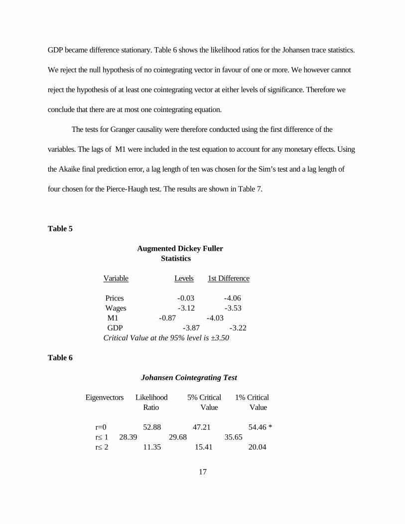
GDP became difference stationary. Table 6 shows the likelihood ratios for the Johansen trace statistics.
We reject the null hypothesis of no cointegrating vector in favour of one or more. We however cannot
reject the hypothesis of at least one cointegrating vector at either levels of significance. Therefore we
conclude that there are at most one cointegrating equation.
The tests for Granger causality were therefore conducted using the first difference of the
variables. The lags of M1 were included in the test equation to account for any monetary effects. Using
the Akaike final prediction error, a lag length of ten was chosen for the Sim’s test and a lag length of
four chosen for the Pierce-Haugh test. The results are shown in Table 7.
Table 5
Augmented Dickey Fuller Statistics Variable Levels 1st Difference Prices -0.03 -4.06 Wages -3.12 -3.53 M1 -0.87 -4.03 GDP -3.87 -3.22 Critical Value at the 95% level is ±3.50 Table 6
Johansen Cointegrating Test
Eigenvectors Likelihood 5% Critical 1% Critical Ratio Value Value
r=0 52.88 47.21 54.46 * r≤ 1 28.39 29.68 35.65 r≤ 2 11.35 15.41 20.04

18
r≤ 3 0.04 3.76 6.65
The F-statistics from the Pierce-Haugh version reveals that wages in fact doesn’t fail to cause
inflation. When performed in reverse the tests show that price inflation fails to cause wage inflation. The
stronger results from the Sim’s tests suggest some contemporaneous relation between wage increases
and inflation. Whereby wages do impact on price, with some feedback effects, in which past price
changes influence the wage setting process.
Table 8 gives the long run results of the modified Harberger model. In all these equations all the
variables exhibit the correct signs and in the first two equations, only the current monetary measure was
significantly different from zero. The coefficients of the change in output/income are not significantly
different from one, indicating that a one percent increase in output/income leads to a more than one
percent fall in prices.
Table 7 Granger Causality F-statistics* Pierce-Haugh Sims Wages vs Prices 2.2922 1.9381 (0.043) (0.317) Prices vs wages 0.2293 1.13072 (0.921) (0.448) *The figures in parentheses denote the probability at the 95% level .

19
Table 8
Dependent Variable: p
Constant pt-1 gdp m1 w a adjR2 DW Akaike ρ --------------------------------------------------------------------------------------------------------------------------------------- [1] 21.959 -1.669 0.225 0.84 1.15 4.3 0.87 (2.3) (1.4) (2.9) (12.25) [2] 6.2 0.585 -0.881 0.207 0.89 1.9 3.99 0.63 (1.5) (5.9) (-1.09) (2.97) (2.9) [3] 5.562 0.615 -0.765 0.195 0.541 0.90 1.9 4.0 0.62 (1.34) (5.9) (-0.95) (2.73) (0.77) (2.7) --------------------------------------------------------------------------------------------------------------------------------------- [3] LM(AR1) χ2 (1) = 3.35 D-F = -4.4 --------------------------------------------------------------------------------------------------------------------------------------- Where p = CPI gdp = rate of growth of real gross domestic product m1 = growth rate in m1 at lag i wa = growth rate in autonomous wage changes.
When the acceleration factor (pt-1) was added, it was significant at the 5.0 percent level with the
monetary variable remaining significant. When the change in wages was added however, it was not
significant. The Akaike criteria suggest a slight preference for equation [2]. These results lead to an
acceptance of hypothesis (1). It should be noted that the Cochrane-Orcutt procedure had to be used as
the lagged dependent variable has a specific definition in the Harberger model. The results for equation
[1] however do suggest the presence of mis-specified dynamics.
The Dickey-Fuller statistics suggests that the residuals of equation [3] are stationary and thus the
variables form a possible cointegrating set. Hendry’s mehtodology of general to specific modelling was
applied in estimating the ECM for equation [3]. Bewley’s transformation was done to correct for small

20
sample bias. The results are given in Table 9.
Table 9 Dependent Variable: Dp Variable Coefficient Std. Error t-Statistics ____________________________________________________________________ Constant -0.2333 0.746 - 0.31 Dp{1} 0.313 0.104 3.01 Dp{2) 0.455 0.12 3.79 Dp(3) 0.106 0.11 0.96 Dp(4) -0.421 0.11 - 3.83 Dm1 0.115 0.046 2.95 Dgdp -2.85 1.271 -2.20 Dgdp{1} 0.301 1.22 0.25 Dwa 1.868 0.612 3.05 Dwa{1} 2.5 0.74 3.38 Dwa{2} 2.45 0.61 4.02 EC{1} -0.231 0.074 -3.12 ___________________________________________________________________ D-F = -4.7 RM F(3, 37) = 2.67265 B-G Lm χ2(1) = 2.845 Engle χ2(1) = 0.2967 B-P Lm χ2(11) = 10.00 J-B χ2(2) = 1.4 ____________________________________________________________________
The Dickey-Fuller statistics (D-F) implies stationarity whilst the Ramseys-RESET test (RM)
indicates correct functional form. The Bruesch-Godfery test (B-G LM) for first order serial correlation
indicates an absence of serial correlation. The Engle ARCH test (Engle) and the Bruesch-Pagan (B-P
LM) tests suggest that the residuals are homoskedastic. The Jarque-Bera statistics with two degrees of
freedom and the significance of the first, third and fourth moments indicate that the residuals are fairly
normal.
The set of the lagged dependent variables seem to be acting as proxies for the effects of omitted
such as exchange rate changes and past changes in the money stock. A more robust specification
therefore would include such variables. What is critical however is that only the first two and fourth lags

21
are significant. This could be what current and lagged wages are responding to in the short run. Although
there maybe some omitted variable bias the coefficient on current GDP is highly significant, and suggests
that current output constraints significantly impact on inflation.
The error correction model implies that whilst we may accept hypothesis (1) in the long run,
both demand and cost pressures arising from structural factors (wages), operate in the short run. We
may conclude that wages have a direct and transmitting role and not necessarily an initiating role. The
lagged responses in Table 10 may imply that wages are reacting to recent changes in prices, money
supply, exchange rate etc. (In fact when the additional lagged dependent variables were dropped, the
wage variables were insignificant.) Since only the current monetary measure is significant, we may infer
that at any time period t, there is monetary accommodation of previous wage adjustments.
Conclusion :
It is clear that higher wages do increase costs, and in the context of less than perfect markets
they impact directly on prices. At the same time however, wage increases generate an increase in
aggregate demand. The question is, in the Jamaican context where productivity and hence output levels
are low, how can these wage increases arise in the first place and secondly how are they sustained (i.e.
how are wage increases financed in the economy). The fact is that increases must be financed or
accommodated somewhere. This is done either by expansion in the money supply or adjustments in
employment levels. The above results imply that this is done primarily in the money market i.e, changes
in the money supply. (This is plausible since the unemployment rate over the years has been more or less
stable.) The process is really a spiral. “Excessive cash holdings are translated first into consumer

22
demand, then into higher prices, and then into higher wages and then into higher demand.”
The stylized solution posited is the creation of a social contract and/or an income policy.
The impact of income policies depends on the means by which inflation is generated. Income policies
will only be useful if inflation is caused be wage settlements outside of market forces. The central appeal
of income policies is that they reduce inflationary expectations. This may not be sufficient however in the
context of expansionary monetary and fiscal policies. Therefore, to be effective, an income policy must
be anchored by appropriate monetary and fiscal policies.
The experience of Jamaica is that attempts at social contracts have not yielded desired results. The
reasons cited have overlooked an essential issue - in the presence of persistent inflation such an
arrangement is subject to the prisoner’s dilemma. This arises from the fact that if workers agree to a
particular wage level then it is in the government’s best interest to expand the money supply so as to
expand output and employment (a socially desirable outcome). This however is not optimal as it is
inflationary. Workers knowing this will therefore demand higher nominal wages. The situation is more
acute when the government lacks credibility. Thus a nash equilibrium will result, in which both parties
will renege on their agreement.
The solution to the problem however, lies in the nature of the equilibrium. Firstly there are no
dominant strategies which the parties may adopt and the nash equilibrium is not unique. . Consequently
we can avoid the prisoner’s dilemma if there is a proper incentive scheme and if there is some means of
ensuring that commitments are binding. This is the typical problem of time inconsistent economic
policy.
The solution would therefore seem to be more institutional in which the government would be

23
bonded to its agreement and workers would be compensated not only in terms of a minimum living
standard but also for the efforts given in achieving the desirable outcome - growth in output9. Thus
practically, the solution and hence the basis of any pact, is a comprehensive productivity incentive
scheme and an institutional framework in which fosters macroeconomic stability.
Possible institutional mechanisms include central bank autonomy, an efficient public sector,
which ensures proper fiscal management and centralized wage negotiation. With respect to the latter, a
major source of instability, even at the firm level, is the multiple bargaining agents. As Alesina and Perotti
(1995) note, “in a centralized nation-wide negotiation with the involvement of the government, the
unions are much more likely to take into consideration the macroeconomic constraints and the adverse
effects of wage increases on labour costs and employment. For many observers, the ability to internalize
the macro effects of wage agreements is precisely what distinguishes the bargaining process in highly
centralized labour markets.”10 Calmfors and Driffill (1993) go on to make the observation that, “the
success of countries such as Sweden, Norway and Austria in maintaining high levels of employment is
usually attributed to centralized bargaining”11
9 In this situtation the participation constraint (minimum individual rationalitty constraint)
and the incentive compatibility constraint is satisfied.
10Alesina and Perotti (1995). Pg3
11Calmfors and Driffill, (1988) pg 28

24
Reference
[1] Alesina A., Perotti, R., The Welfare State and Competitiveness. mimeo (1995)
[2] Calmfors L., and Driffill J., Bargaining Structure, Corporatism and Macroeconomic Performance. Economic Policy (1993) [3] Downes, A. et al The Wage-Price Productivity Relationship in a Small Developing Economy: The case of Barbados. Social and Economic Studies vol. 39 1990. [4] Frisch, H., Theories of Inflation Cambridge Survey of Economic Literature. Cambridge 1983. [5] Granger C.W., Investigating Causal Relationships by Econometric Models and Cross Spectral Models. Econometrica (1969) vol 37, pg. 424-438 [6] Griffiths B., Inflation, Morrison & Gibbs Ltd. London (1976).
[7] Guillermo C.A., Inflation in Jamaica: causes and cures. Mimeo Bank of Jamaica (1994)

25
[8] Hoel M., Union Wage Policy: The Importance of Labour mobility and the Degree of Centralization. Economica vol.58 (1991) [9] Koot, R., A Test for Demand-Pull or Wage-Push Inflation. Social and Economic Studies, Vo. 17 No. 2 June 1968. [10] Laidler, D.E., Essays on Money and Inflation. University of Chicago Press. Chicago 1975. [11] Latibeaudiere, D., An Analysis of Inflation in Jamaica. Bank of Jamaica. 1974. [12] Lewis A., Jamaica’s Economic problems, Daily Gleaner, September 1964.
[13] Ministry of Labour Annual Reports [14] Sims C.A., Money and Income Causality. American Economic Review vol. 62 (1972).
pg. 540-552 [15] __________ Macroeconomics and Reality. Econometrica vol. 49 (1980) pg.1-49 [16] Statistical Institute of Jamaica, National Income and Product (various issues) [17] _____________________ Consumer Price Index (various issues) [18] _____________________ Labour Force Statistics (various issues) [19] _____________________ Employment, Earnings and Hours Worked in Large Establishments (various issues) [20] Thomas, D., Estimating a Monetary Model of Inflation Determination in Jamaica. Regional Programme of Monetary Studies 1994. [21] Witter, M., Reid, R., The Inflationary Impact of Wage Increases in the Jamaican Economy. U.W.I. 1995