lagrangian analysis of two- and three-dimensional … · lagrangian analysis of two- and...
TRANSCRIPT

LagrangianAnalysis ofTwo- and
Three-Dimensional
Oceanic Flowsfrom EulerianVelocity Data
David Russell
Introduction
Approach andAlgorithms
Implementation
Validation
Application
Schedule
Deliverables
Bibliography
Lagrangian Analysis of Two- andThree-Dimensional Oceanic Flows from Eulerian
Velocity Data
David RussellSecond-year Ph.D. student, Applied Math and Scientific Computing
Project Advisor: Kayo IdeDepartment of Atmospheric and Oceanic Science
Center for Scientific Computation and Mathematical ModelingEarth System Science Interdisciplinary CenterInstitute for Physical Science and Technology
October 6, 2015

LagrangianAnalysis ofTwo- and
Three-Dimensional
Oceanic Flowsfrom EulerianVelocity Data
David Russell
Introduction
Approach andAlgorithms
Implementation
Validation
Application
Schedule
Deliverables
Bibliography
Introduction
Atmospheric flows have various coherent structures, suchas fronts, jet streams, and hurricanes
Clouds often provide a ready means of visually trackingthese flows

LagrangianAnalysis ofTwo- and
Three-Dimensional
Oceanic Flowsfrom EulerianVelocity Data
David Russell
Introduction
Approach andAlgorithms
Implementation
Validation
Application
Schedule
Deliverables
Bibliography
Introduction
The oceans have nobuilt-in “tracers” to trackthe flow, so their structureremains largely hidden
Grid-based computermodels can generatevelocity data at certaindiscrete points in spaceand time, but these dataalone do not revealcoherent structures in theflow

LagrangianAnalysis ofTwo- and
Three-Dimensional
Oceanic Flowsfrom EulerianVelocity Data
David Russell
Introduction
Approach andAlgorithms
Implementation
Validation
Application
Schedule
Deliverables
Bibliography
Introduction
To better visualize the underlying structures, we can laydown a network of particles and track them as they movethrough the flow
Using certain quantitative analysis tools to color theparticles, we can clearly delineate coherent structures, aswell as the manifolds (boundaries) that separate them
We can also use these tools as a launching point for adeeper investigation of the mixing and transport propertiesof a given flow

LagrangianAnalysis ofTwo- and
Three-Dimensional
Oceanic Flowsfrom EulerianVelocity Data
David Russell
Introduction
Approach andAlgorithms
Implementation
Validation
Application
Schedule
Deliverables
Bibliography
Introduction
Example: Kuroshio current, northwest Pacific Ocean
Red indicates faster-moving regions, blue slowerThin yellowish lines represent stable and unstablemanifoldsCoherent structures clearly visible

LagrangianAnalysis ofTwo- and
Three-Dimensional
Oceanic Flowsfrom EulerianVelocity Data
David Russell
Introduction
Approach andAlgorithms
Implementation
Validation
Application
Schedule
Deliverables
Bibliography
Introduction
This approach entails a shift from an “Eulerian” to a“Lagrangian” perspective:
Eulerian: Track fluid velocity from a fixed point in space(e.g. an observing station)Lagrangrian: Track fluid velocity following a tiny parcel offluid as it moves through the flow

LagrangianAnalysis ofTwo- and
Three-Dimensional
Oceanic Flowsfrom EulerianVelocity Data
David Russell
Introduction
Approach andAlgorithms
Implementation
Validation
Application
Schedule
Deliverables
Bibliography
Introduction
Our goals for this project are:
Given a two- or three-dimensional velocity dataset in thisEulerian form, convert it to a Lagrangian form bycalculating trajectories for a large number of particles laidout in a latticeDesign tools to visualize and analyze the flow structuresbased on this Lagrangian dataApply these tools to a flow field from a computer model ofthe Chesapeake Bay, see what we can learn about itstransport and mixing properties

LagrangianAnalysis ofTwo- and
Three-Dimensional
Oceanic Flowsfrom EulerianVelocity Data
David Russell
Introduction
Approach andAlgorithms
Implementation
Validation
Application
Schedule
Deliverables
Bibliography
Approach
XXX (XXX 0, t) is (2D or 3D) position of particle at time t thatbegan at position XXX 0
uuu(xxx , t) is velocity field at position xxx at time t
2D: uuu(xxx , t) = (u(x , y , t), v(x , y , t))3D: uuu(xxx , t) = (u(x , y , z , t), v(x , y , z , t),w(x , y , z , t))
These quantities must be related by dXXXdt (XXX 0, t) = uuu(XXX 0, t)
In practice, however, model only gives uuu at discrete gridpoints, say (xi , yj , zk , tl) in 3D
Particles travel between grid points (in time and space), sowe need a way to interpolate uuu to these non-grid points

LagrangianAnalysis ofTwo- and
Three-Dimensional
Oceanic Flowsfrom EulerianVelocity Data
David Russell
Introduction
Approach andAlgorithms
Implementation
Validation
Application
Schedule
Deliverables
Bibliography
Velocity Interpolation
Horizontal spatial interpolation: Bilinear interpolation(simplest method)
Approximate velocity within eachgrid box by a function of the formf (x , y) = c1 + c2x + c3y + c4xy(four constants determined byknown values at corners)
Not very accurate (first-order), notsmooth, but fast

LagrangianAnalysis ofTwo- and
Three-Dimensional
Oceanic Flowsfrom EulerianVelocity Data
David Russell
Introduction
Approach andAlgorithms
Implementation
Validation
Application
Schedule
Deliverables
Bibliography
Velocity Interpolation
Horizontal spatial interpolation: Bicubic interpolation(higher-order method)
Approximate by a function of theform f (x , y) =
∑3i=0
∑3j=0 cijx
iy j
16 unknowns, so we also needapproximations of fx , fy , and fxy atthe corners (can get these usingcentered difference approximations)
Smoother and more accurate, butslower

LagrangianAnalysis ofTwo- and
Three-Dimensional
Oceanic Flowsfrom EulerianVelocity Data
David Russell
Introduction
Approach andAlgorithms
Implementation
Validation
Application
Schedule
Deliverables
Bibliography
Velocity Interpolation
Vertical spatial interpolation (for 3D)
Low-order method: Interpolate linearly from horizontalinterpolationHigher-order method: Use cubic polynomial passingthrough four nearest points?
Time interpolation
Low-order method: Interpolate linearly from spatialinterpolationHigh-order method: Use cubic polynomial passing throughfour nearest points?

LagrangianAnalysis ofTwo- and
Three-Dimensional
Oceanic Flowsfrom EulerianVelocity Data
David Russell
Introduction
Approach andAlgorithms
Implementation
Validation
Application
Schedule
Deliverables
Bibliography
Time Integration
After interpolating uuu to a desired particle position, wemust evolve this position in time by solving the system
dX
dt= u(X ,Y , t)
dY
dt= v(X ,Y , t)
or
dX
dt= u(X ,Y ,Z , t)
dY
dt= v(X ,Y ,Z , t)
dZ
dt= w(X ,Y ,Z , t)
Low-order method: Forward Euler (first-order)
High-order method: 4th-order predictor-corrector usingMilne for predictor and Hamming for corrector
RK4 also a simpler higher-order option

LagrangianAnalysis ofTwo- and
Three-Dimensional
Oceanic Flowsfrom EulerianVelocity Data
David Russell
Introduction
Approach andAlgorithms
Implementation
Validation
Application
Schedule
Deliverables
Bibliography
Lagrangian Analysis Tools
Once we have our particle trajectories, we can calculatesome useful functions for analyzing the flow
M-function: Calculates the arc length of a given trajectoryover a prescribed time period (forward and backward bytime τ):
Muuu,τ (XXX ∗0, t
∗) =
∫ t∗+τ
t∗−τ
(2 or 3∑i=1
(dXi (t)
dt
)2) 1
2
dt
M-function proportional to average speed near time t∗, soif we color particles by M-function, different colors willindicate different flow speeds

LagrangianAnalysis ofTwo- and
Three-Dimensional
Oceanic Flowsfrom EulerianVelocity Data
David Russell
Introduction
Approach andAlgorithms
Implementation
Validation
Application
Schedule
Deliverables
Bibliography
Lagrangian Analysis Tools
Finite-Time Lyapunov Exponent (FTLE): Measures thedegree to which two nearby trajectories diverge over time
if δXXX 0 represents an infinitesimal displacement betweentwo nearby particles, then for certain directions, |δXXX 0| willgrow or shrink exponentially in time, i.e.|δXXX (t)| ≈ eλt |δXXX 0|(Maximum) FTLE is defined as the largest such growthrate λ
FTLE grows large when flow bifurcates, so coloring byFTLE should also reveal coherent structures

LagrangianAnalysis ofTwo- and
Three-Dimensional
Oceanic Flowsfrom EulerianVelocity Data
David Russell
Introduction
Approach andAlgorithms
Implementation
Validation
Application
Schedule
Deliverables
Bibliography
Finite-Time Lyapunov Exponent

LagrangianAnalysis ofTwo- and
Three-Dimensional
Oceanic Flowsfrom EulerianVelocity Data
David Russell
Introduction
Approach andAlgorithms
Implementation
Validation
Application
Schedule
Deliverables
Bibliography
Finite-Time Lyapunov Exponent
To calculate the FTLE at a given time t, let L = ∂XXX (t)∂XXX 0
bethe transition matrix (Jacobian of position with respect toinitial position)
FTLE is given by
λ ≈ 1
tln (largest singular value of L)
=1
2tln(
largest eigenvalue of LTL)
So to calculate λ, we need to approximate L as well asfind the eigenvalues of a 2x2 or 3x3 matrix
LagrangianAnalysis ofTwo- and
Three-Dimensional
Oceanic Flowsfrom EulerianVelocity Data
David Russell
Introduction
Approach andAlgorithms
Implementation
Validation
Application
Schedule
Deliverables
Bibliography
Finite-Time Lyapunov Exponent
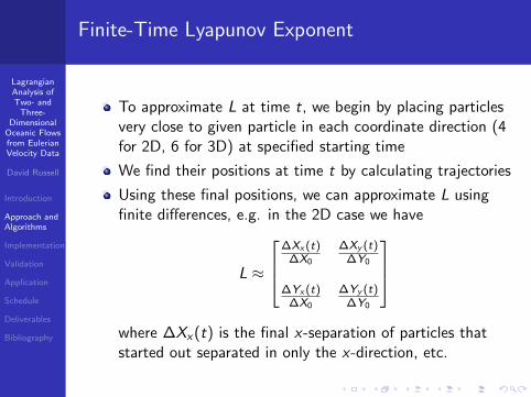
To approximate L at time t, we begin by placing particlesvery close to given particle in each coordinate direction (4for 2D, 6 for 3D) at specified starting time
We find their positions at time t by calculating trajectories
Using these final positions, we can approximate L usingfinite differences, e.g. in the 2D case we have
L ≈
∆Xx (t)
∆X0
∆Xy (t)∆Y0
∆Yx (t)∆X0
∆Yy (t)∆Y0
where ∆Xx(t) is the final x-separation of particles thatstarted out separated in only the x-direction, etc.

LagrangianAnalysis ofTwo- and
Three-Dimensional
Oceanic Flowsfrom EulerianVelocity Data
David Russell
Introduction
Approach andAlgorithms
Implementation
Validation
Application
Schedule
Deliverables
Bibliography
Finite-Time Lyapunov Exponents
To calculate the eigenvalues of the 2x2 or 3x3 matrix L,we must solve its characteristic equation
2D: The characteristic equation is quadratic, so we cansimply use the quadratic formula
3D: The characteristic equation is cubic, so we must writea cubic solver (based on Newton’s method?)

LagrangianAnalysis ofTwo- and
Three-Dimensional
Oceanic Flowsfrom EulerianVelocity Data
David Russell
Introduction
Approach andAlgorithms
Implementation
Validation
Application
Schedule
Deliverables
Bibliography
Implementation
Software: MATLAB
Hardware: MacBook Pro laptop (mid-2014), 2.6 GHz IntelCore i5, 8 GB RAM (can access Deepthought2 HPCcluster on campus if necessary)
Circa 800,000 particles to track, so trajectorycomputations will get very expensive
However, each trajectory is independent, so all calculationscan be done in parallel
Can investigate accuracy vs. speed tradeoff forinterpolation and integration algorithms

LagrangianAnalysis ofTwo- and
Three-Dimensional
Oceanic Flowsfrom EulerianVelocity Data
David Russell
Introduction
Approach andAlgorithms
Implementation
Validation
Application
Schedule
Deliverables
Bibliography
Validation
Validate our tools by testing them on a few dynamicalsystems with well known phase portraits (stable andunstable manifolds, typical trajectories, etc.)
Evaluate velocity for each of these systems on a fineenough grid, then feed this velocity data into ourLagrangian routines
Routines should reproduce the known phase portraits

LagrangianAnalysis ofTwo- and
Three-Dimensional
Oceanic Flowsfrom EulerianVelocity Data
David Russell
Introduction
Approach andAlgorithms
Implementation
Validation
Application
Schedule
Deliverables
Bibliography
Test Problems
Forced and unforced Duffing oscillator
dx
dt= y
dy
dt= x − x3 + ε sin t
(set ε = 0 for unforced)

LagrangianAnalysis ofTwo- and
Three-Dimensional
Oceanic Flowsfrom EulerianVelocity Data
David Russell
Introduction
Approach andAlgorithms
Implementation
Validation
Application
Schedule
Deliverables
Bibliography
Test Problems
Three-variable Lorenz equations
dx
dt= σ(y − x)
dy
dt= rx − y − xz
dz
dt= xy − bz

LagrangianAnalysis ofTwo- and
Three-Dimensional
Oceanic Flowsfrom EulerianVelocity Data
David Russell
Introduction
Approach andAlgorithms
Implementation
Validation
Application
Schedule
Deliverables
Bibliography
Test Problems
Hill’s spherical vortex
ψ = −3
4Ur2
(1− r2
a2
)sin2 θ
ur =1
r2 sin θ
∂ψ
∂θ
uθ = − 1
r sin θ
∂ψ
∂r

LagrangianAnalysis ofTwo- and
Three-Dimensional
Oceanic Flowsfrom EulerianVelocity Data
David Russell
Introduction
Approach andAlgorithms
Implementation
Validation
Application
Schedule
Deliverables
Bibliography
Application
Apply tools to velocitydata for the ChesapeakeBay
Data is output from aROMS (Regional OceanModeling System) modelof the bay
Tools must be able tohandle ROMSspecifications

LagrangianAnalysis ofTwo- and
Three-Dimensional
Oceanic Flowsfrom EulerianVelocity Data
David Russell
Introduction
Approach andAlgorithms
Implementation
Validation
Application
Schedule
Deliverables
Bibliography
Regional Ocean Modeling System
ROMS is a free-surface,terrain-following, primitiveequations ocean modelthat can be adapted tovarious regions
Chesapeake ROMS usescurvilinear coordinatestailored to geography
All algorithms will beapplied in this coordinatesystem

LagrangianAnalysis ofTwo- and
Three-Dimensional
Oceanic Flowsfrom EulerianVelocity Data
David Russell
Introduction
Approach andAlgorithms
Implementation
Validation
Application
Schedule
Deliverables
Bibliography
Regional Ocean Modeling System
Grid type is so-called Arakawa C-grid (u, v , and wevaluated on different faces of each grid box)
This means u, v , and w will be interpolated relative todifferent grids
Boundary conditions: no-slip (uuu = 0 at boundary) orfree-slip (uuu · n̂nn = 0 at boundary)

LagrangianAnalysis ofTwo- and
Three-Dimensional
Oceanic Flowsfrom EulerianVelocity Data
David Russell
Introduction
Approach andAlgorithms
Implementation
Validation
Application
Schedule
Deliverables
Bibliography
Application
Expect M-function and FTLE data to reveal coherentstructures in Chesapeake Bay dataset
Use Chesapeake ROMS data as one more validation test(test everything against results of another researcher ingroup)
Time permitting, use Lagrangian tools to quantitativelyinvestigate transport and mixing processes, e. g.:
What percentage of the water entering the bay fromrivers/ocean also exits through the rivers/ocean within acertain timeframe?Can we observe and quantify dynamic effects of Coriolisforce, density differences between ocean and fresh water,etc.

LagrangianAnalysis ofTwo- and
Three-Dimensional
Oceanic Flowsfrom EulerianVelocity Data
David Russell
Introduction
Approach andAlgorithms
Implementation
Validation
Application
Schedule
Deliverables
Bibliography
Expected Visualization Results

LagrangianAnalysis ofTwo- and
Three-Dimensional
Oceanic Flowsfrom EulerianVelocity Data
David Russell
Introduction
Approach andAlgorithms
Implementation
Validation
Application
Schedule
Deliverables
Bibliography
Schedule
First SemesterFirst half: October - Mid-November
Project proposal presentation and paper2D and 3D interpolation
Second half: Mid-November - December
2D trajectory implementation and validationM function implementation and validationMid-year report and presentation
Second SemesterFirst half: January - February
3D trajectory implementation and validationFTLE implementation
Second half: March - April
Visualizations and further analysisFinal presentation and paper

LagrangianAnalysis ofTwo- and
Three-Dimensional
Oceanic Flowsfrom EulerianVelocity Data
David Russell
Introduction
Approach andAlgorithms
Implementation
Validation
Application
Schedule
Deliverables
Bibliography
Deliverables
Code
Routines that lay down particle lattice and calculatetrajectories from velocity dataRoutines that calculate M-function and FTLE based ontrajectories
Results
Series of visualizations (images, movies, graphs) based onthese functions, for Chesapeake Bay data and testproblems

LagrangianAnalysis ofTwo- and
Three-Dimensional
Oceanic Flowsfrom EulerianVelocity Data
David Russell
Introduction
Approach andAlgorithms
Implementation
Validation
Application
Schedule
Deliverables
Bibliography
Deliverables
Reports
Project proposal and presentationMid-year progress report and presentationFinal paper and presentation
Databases
Chesapeake Bay ROMS dataset

LagrangianAnalysis ofTwo- and
Three-Dimensional
Oceanic Flowsfrom EulerianVelocity Data
David Russell
Introduction
Approach andAlgorithms
Implementation
Validation
Application
Schedule
Deliverables
Bibliography
Bibliography
Mancho, A. M., Wiggins S., Curbelo J. & Mendoza, C.(2013). Lagrangian descriptors: A method for revealingphase space structures of general time dependentdynamical systems. Communications in Nonlinear Scienceand Numerical Simulation, 18, pp. 3530-3557.
Mendoza, C. & Mancho, A. M. (2010). Hidden geometryof ocean flows. Physical Review Letters, 105(038501), pp.1-4.
Shadden, S. C., Lekien, F. & Marsden, J. (2005).Definition and properties of Lagrangian coherent structuresfrom finite-time Lyapunov exponents in two-dimensionalaperiodic flows. Physica D, 212, pp. 271-304
Xu, J. et al. (2012). Climate forcing and salinityvariability in Chesapeake Bay, USA. Estuaries and Coasts,35, pp. 237-261.