Lagrangian GSOM traffic flow models on

junctions

Guillaume Costeseque ∗,∗∗ Jean-Patrick Lebacque ∗

Asma Khelifi ∗,∗∗∗

∗ Université Paris-Est, IFSTTAR, GRETTIA, 14-20 BoulevardNewton, Cité Descartes, Champs sur Marne, 77447 Marne la Vallée

Cedex 2, France (e-mail: firstname.lastname@ifsttar.fr)∗∗ Université Paris-Est, Ecole des Ponts ParisTech, CERMICS, 6 & 8

avenue Blaise Pascal, Cité Descartes, Champs sur Marne,77455 Marne la Vallée Cedex 2, France.

∗∗∗ Ecole Nationale d’Ingénieurs de Tunis, Rue Béchir Salem BelkhiriaCampus universitaire, BP 37, 1002 Tunis Belvédère, Tunisie.

Abstract: This paper is concerned with the macroscopic modeling and simulation of traffic flowon junctions. More precisely, we deal with a generic class of second order models, known in theliterature as the GSOM family. While classical approaches focus on the Eulerian point-of-view,here we recast the model using its Lagrangian coordinates and we treat the junction as a specificdiscontinuity in Lagrangian framework. We propose a complete numerical methodology basedon a finite difference scheme for solving such a model and we provide a numerical example.

Keywords: Traffic flow; junction; GSOM models; Lagrangian; numerical scheme.

1. INTRODUCTION

1.1 Motivation

In this paper, we are motivated by road network modeling,thanks to macroscopic traffic flow models. First ordertraffic flow models have been used for quite a long timefor modeling traffic flows on networks (see Garavelloand Piccoli (2006); Lebacque and Khoshyaran (2002) forinstance). In particular, the seminal LWR model standingfor Lighthill and Whitham (1955); Richards (1956) hasbeen widely used. However, first order models do notallow to recapture accurately specific and meaningfultraffic flow phenomena. Thus we focus on the GenericSecond Order Models (GSOM) family which encompassesa large variety of higher order traffic flow models. GSOMmodels have been already well studied on homogeneoussections but they have attracted little attention for theirimplementation on junctions, as it is discussed in Section 3.However, junctions are the main source of congestion fortraffic streams on a network.

In this paper, we want to develop a junction modelwhich is compatible with microscopic and macroscopicdescriptions, and satisfies classical constraints coming fromengineering, as for instance the invariance principle dis-cussed in Lebacque and Khoshyaran (2005); Tampère et al.(2011); Costeseque and Lebacque (2014a). The micro-scopic representation of traffic flow is particularly suitedfor traffic management methods, while staying compatiblewith a macroscopic representation allowing global evalu-ation. The key idea for conciliating both microscopic and

⋆ This work was partially supported by the ANR (Agence Nationalede la Recherche) through HJnet project ANR-12-BS01-0008-01.

macroscopic representations is to recast the macroscopicmodel under its Lagrangian coordinates. Indeed the La-grangian framework focuses directly on the particles andincidentally it allows to keep track of individual behaviors(see for instance Leclercq et al. (2007) in the case of firstorder LWR model).

1.2 Organization of the paper

The article is organized as follows. In Section 2, the genericclass of second order macroscopic traffic flow models calledGSOM family, is introduced. In Section 3, we review anddiscuss the literature for solving GSOM models posedon junctions. Our aim is to show that the Lagrangianframework is well-suited for designing the solution toGSOM problems even if incorporating discontinuities. Thecomplete numerical methodology is described in Section 4and a numerical example is given incidentally in Section 5.Finally, we provide some conclusions on this work and givesome insights on future research in Section 6.

2. GSOM FAMILY

2.1 Formulation of GSOM models

In Lebacque et al. (2005, 2007), the authors introduce ageneral class of macroscopic traffic flow models called theGeneric Second Order Models (GSOM) family. Assumethat ρ(t, x) stands for the density of vehicles at locationx ∈ R and time t ≥ 0. Any model of the GSOM familycan be stated in conservation form as follows

∂

∂t

(

ρρI

)

+∂

∂x

(

ρvρvI

)

=

(

0ρϕ(I)

)

, on (0, +∞)×R, (1)

8th Vienna International Conference on Mathematical ModellingFebruary 18 - 20, 2015. Vienna University of Technology, Vienna,Austria

Copyright © 2015, IFAC 147

with the initial conditions{

ρ(0, x) = ρ0(x), on R,

I(0, x) = I0(x), on R.

The speed is defined by v := I(ρ, I) where I denotes thespeed-density Fundamental Diagram (FD) which dependson the choice of the GSOM model. It is usually assumedto be non-increasing with respect to its first variable. Theflow-density FD is then defined by

F : (ρ, I) 7→ ρI(ρ, I). (2)

The variable I(N(t, x)) ∈ Rm, for some m ∈ N, represents

an attribute which is specific to the vehicle N locatedat position x and time t. This attribute (which is laterdenoted I(t, x) by abuse of notation) can represent, forinstance, the driver aggressiveness, the driver destinationor the vehicle class. The function ϕ : I 7→ ϕ(I) accountsfor the dynamics of the attribute I.

The GSOM family recovers a wide range of existing modelsamong which there is the LWR model of Lighthill andWhitham (1955); Richards (1956), a GSOM model withno specific driver attribute (I = κ for any κ ∈ R),

{

∂tρ + ∂x(ρv) = 0 on (0, +∞)× R,

ρ(0, x) = ρ0(x), on R(3)

and the ARZ model (Aw and Rascle (2000) and Zhang(2002)) for which the driver attribute is taken as thedifference between actual speed and the equilibrium speedVe(ρ) depending only on the density, that is I = v−Ve(ρ).The speed-density FD boils down to I(ρ, I) = I + Ve(ρ).

The interested reader is referred to Lebacque and Khosh-yaran (2013) and references therein for more details onother examples.

2.2 A note on Supply-Demand functions

It is worth noticing that the notions of supply and demandfunctions defined in Lebacque (1996) for the classical LWRmodel (3) and expanded to the case of the LWR model onjunctions in Lebacque and Khoshyaran (2002), could bealso extended to the GSOM family, as it was shown inLebacque et al. (2007). These functions built on the flow-density FD are essential to build monotone finite volumeschemes for solving the hyperbolic system (1). Supply anddemand functions are also particularly relevant for trafficflow modeling through junctions.

If F denotes the flow-density FD defined in (2) (by ex-tension of notation, we will consider F(., .; x) as the flow-density FD at position x ∈ R), then equilibrium demandand supply functions are defined as follows

∆ (ρ, I; x) := max0≤k≤ρ

F(

k, I; x−)

,

Σ (ρ, I; x) := maxk≥ρ

F(

k, I; x+) (4)

where x+ (resp. x−) denotes the upper (resp. lower) limit.

In the case of GSOM models, the extension of local trafficsupply and demand definitions is far from being straight-forward. Indeed, it has been pointed out in Lebacque et al.(2007) that downstream supply depends on the upstreamdriver attribute (which has not already passed through the

considered point). The upstream demand and downstreamsupply at a point x and time t are defined such that

{

δ(x, t) := ∆(

ρ(x−, t), I(x−, t); x)

,

σ(x, t) := Σ(

ρ(x, t), I(x+, t); x)

,(5)

with

ρ(x, t) := I−1{

I(

ρ(x+, t), I(x+, t); x+)

, I(x−, t); x+}

.(6)

Then the passing flow at location x, time t is given by thecelebrated Min formula

q(t, x) = min {δ(t, x), σ(t, x)} .

I

I(., I−)

I(., I+)

v := I(ρ+, I+)

ρ̄ := I−1(v, I−)ρ+

ρ

Fig. 1. The downstream supply depends on the upstreamdriver attribute. Here, we have defined I+ := I(x+, t),I− := I(x−, t) and ρ+ := ρ(x+, t).

Let us introduce the modified demand for the GSOMmodels as follows

Ξ (ρ, I1, I2; x) := Σ(

I−1{

I(

ρ, I2; x+)

, I1; x+}

, I2; x)

,(7)

such that (5)-(6) boil down to

σ(x, t) := Ξ(

ρ(x, t), I(x+, t), I(x−, t); x)

.

2.3 Lagrangian setting of the GSOM family

The common expression of GSOM models in Euleriancoordinates (t, x) is given by (1). However, it is well-knownthat Lagrangian framework (t, n) is particularly conve-nient for dealing with flows of particles and it is especiallytrue in traffic flow modeling (see Leclercq et al. (2007); vanWageningen-Kessels et al. (2013) and references therein).

Assume that N(t, x) ∈ R describes the label of vehicle at

position x and time t. We set the spacing r :=1

ρand the

speed-spacing FD as follows

V(r, I) := I

(

1

r, I

)

for any (r, I) ∈ (0, +∞)× Rm. (8)

If we set the following change of coordinates

N(t, x) :=

∫ +∞

x

ρ(t, ξ)dξ,

T := t

such that

{

∂N = −r∂x,

∂T = ∂t + v∂x

where v denotes the speed of particles, then the GSOMmodel (1) can be recast in Lagrangian form as follows

{

∂T r + ∂NV(r, I) = 0 on (0, +∞)× R,

∂T I = ϕ(I) on (0, +∞)× R,(9)

with initial conditions{

r(0, n) = r0(n), on R,

I(0, n) = I0(n), on R.

MATHMOD 2015February 18 - 20, 2015. Vienna, Austria

148

One can notice also that we have r = −∂NX whereX (T, N) denotes the position of particle N at time T whichsolves the following Hamilton-Jacobi equation

{

∂TX = V (−∂NX , I) ,

∂T I = ϕ(I).(10)

3. BRIEF REVIEW OF THE LITERATURE

There already exist a few works on the Lagrangian model-ing of junctions based on GSOM models; see for instanceMoutari and Rascle (2007); van Wageningen-Kessels et al.(2013); Khoshyaran and Lebacque (2008). However, someof these works are based on very specific examples ex-tracted from the GSOM family. But it is not straightfor-ward to extend the numerical methodologies presented inthese papers to the generic GSOM model (9).

In Khoshyaran and Lebacque (2008), the authors considerthe Godunov scheme applied to (9). The authors extendthis particle discretization to networks, addressing theproblem of junction modeling through a supply-demandapproach. The authors make the choice to introduce aninternal state model (see Lebacque et al. (2008); Khosh-yaran and Lebacque (2009)) and assume that the particlesshare the same attribute once they have passed. By theway, the authors deal also with densities and flows whichis not particularly convenient with GSOM models in theLagrangian framework. Hopefully, dealing with spacinginstead of density will ease the resolution of the model.

While boundary conditions can be treated within theframework of supply-demand flows methodology (seeLebacque et al. (2005, 2007) and Khoshyaran and Lebacque(2008)), expressions of upstream and downstream bound-ary conditions into Lagrangian coordinates can be ob-tained in the framework of variational approach for GSOMmodels (see Lebacque and Khoshyaran (2013)). It will bedeveloped in next section.

4. METHODOLOGY FOR THE LAGRANGIANMODELING OF JUNCTIONS

In this section, we describe the numerical scheme adaptedfor the generic Lagrangian GSOM model (9) posed on ajunction. We partially follow Lebacque and Khoshyaran(2013) in which the authors describe boundary conditionsfor the Hamilton-Jacobi equation (10) associated to theLagrangian GSOM model (9).

We set a junction as the union of NI incoming and NO

outgoing branches that intersect at a unique point calledthe junction point (or the node in the traffic literature).We also define I := J1, NIK (resp. J := JNI +1, NI +NOK)the set of incoming (resp. outgoing) links.

4.1 Lagrangian discretized model

Let us introduce ∆t and ∆N the time and particle stepsrespectively. We set It

n := I(t∆t, n∆N), for any t ∈ N andany n ∈ Z.

We have the choice between two Finite Difference schemes:either we deal with the discrete particle spacing defined as

rtn := r(t∆t, n∆N), for any (t, n) ∈ N× Z,

where r solves the Lagrangian GSOM model (9), or weconsider the discrete particle position that reads

X tn := X (t∆t, n∆N), for any (t, n) ∈ N× Z,

where (X , I) solves the Hamilton-Jacobi problem (10)associated to (9). Notice that the spatial extension ofparticle n ∈ Z is [X t

n,X tn−1[.

In the first case, we would have to solve the followingnumerical scheme for (9)

rt+1n := rt

n +∆t

∆N

[

V tn−1 − V t

n

]

,

V tn := V

(

rtn, It

n

)

,

It+1n = It

n + ∆tϕ(

Itn

)

(11)

while in the second case, i.e. for (10) the appropriatenumerical scheme is defined as follows

X t+1n = X t

n + ∆tV tn ,

V tn := V

(

X tn−1 −X

tn

∆N, It

n

)

,

It+1n = It

n + ∆tϕ(

Itn

)

(12)

Notice that both approaches are very similar and give backthe same results. Indeed, one can remark that if we have

rtn :=

X tn−1 −X

tn

∆N, (13)

then (11) is simply deduced from (12). By the way,knowing the spacing at each numerical steps, it is easyto compute the position of all particles, given the leaderparticle trajectory as a boundary condition.

It is worth noting that both schemes are first orderschemes. The first one (11) can be interpreted as the sem-inal Godunov scheme (see Godunov (1959)) applied withdemand and supply and the second discrete model (12) isan explicit Euler scheme.

In order to the numerical schemes (11) and (12) bemonotone, time and label discrete steps need to satisfya Courant-Friedrichs-Lewy (CFL) condition given by

∆N

∆t≥ sup

N,r,t

|∂rV(r, I(t, N))| . (14)

For deducing a particle (Lagrangian) discretization of atraffic flow model on a junction, it is necessary to takeinto consideration different elements:

(i) the link model, which is given by either (11) or (12);(ii) the upstream (resp. downstream) boundary condi-

tions for any incoming (resp. outgoing) link;(iii) the internal junction model, say the way particles are

assigned from incoming road i ∈ I to outgoing roadj ∈ J and eventually the internal dynamics of thejunction point;

(iv) link-junction and junction-link interfaces.

These constituting elements are addressed in what follows.

4.2 Downstream boundary condition

We assume that we are located at the downstream bound-ary of a given outgoing road j ∈ J . Assume the exit pointS located at xS . The downstream boundary data at xS isgiven by the downstream supply σ which is discretized asσt at time step t. Let n be the last particle located on the

MATHMOD 2015February 18 - 20, 2015. Vienna, Austria

149

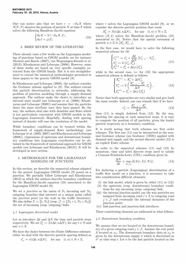
link (or at least a fraction η∆N of it is still on the link,with 0 < η ≤ 1). See Figure 2.

rtn∆N

xS

n− 1

X tn

r∗r∗ rcrit(I)

σt

V(., I)

r

n

Fig. 2. Illustration of downstream boundary condition.

We define the spacing associated to particle n as

rtn :=

xS −Xtn

η∆N.

The fraction η is instantiated at the first time step tn

following the exit of particle (n− 1), as follows

η =xS −X

tn

n

rtn

n ∆N.

Now, we have to distinguish two cases:

• either V(rtn, It

n) ≤ σtrtn: in this case, the downstream

supply is sufficient to accommodate the demand onthe link. The spacing is conserved.• or V(rt

n, Itn) > σtrt

n: in this case, the demand on thelink cannot be fully satisfied since the downstreamsupply limits the outflow. Then, we have to solve

V(rtn, It

n) = σtrtn

and we choose the smallest value i.e. rtn = r∗ (see

Figure 2). It means that we select the solution corre-sponding to the congested phase.

Then, we still update the position of particle n as usual,using (12). We also need to update the fraction η if theparticle has not totally exited the link i.e. if X t+1

n < xS .The updated fraction is computed as follows

η ← η −∆t

rtn∆N

V(

rtn, It

n

)

.

4.3 Upstream boundary conditions

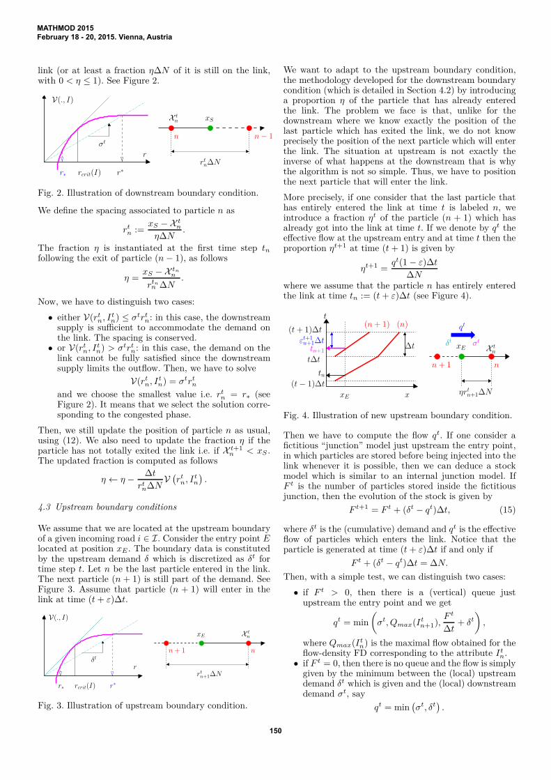
We assume that we are located at the upstream boundaryof a given incoming road i ∈ I. Consider the entry point Elocated at position xE . The boundary data is constitutedby the upstream demand δ which is discretized as δt fortime step t. Let n be the last particle entered in the link.The next particle (n + 1) is still part of the demand. SeeFigure 3. Assume that particle (n + 1) will enter in thelink at time (t + ε)∆t.

δt

nn + 1

rtn+1∆N

r∗ r∗rcrit(I)

V(., I)

r

xE X tn

Fig. 3. Illustration of upstream boundary condition.

We want to adapt to the upstream boundary condition,the methodology developed for the downstream boundarycondition (which is detailed in Section 4.2) by introducinga proportion η of the particle that has already enteredthe link. The problem we face is that, unlike for thedownstream where we know exactly the position of thelast particle which has exited the link, we do not knowprecisely the position of the next particle which will enterthe link. The situation at upstream is not exactly theinverse of what happens at the downstream that is whythe algorithm is not so simple. Thus, we have to positionthe next particle that will enter the link.

More precisely, if one consider that the last particle thathas entirely entered the link at time t is labeled n, weintroduce a fraction ηt of the particle (n + 1) which hasalready got into the link at time t. If we denote by qt theeffective flow at the upstream entry and at time t then theproportion ηt+1 at time (t + 1) is given by

ηt+1 =qt(1− ε)∆t

∆N

where we assume that the particle n has entirely enteredthe link at time tn := (t + ε)∆t (see Figure 4).

εt+1n+1∆t

qt

(t− 1)∆t

tn

(n + 1)

xE

(n)

x

∆t xE X tn

ηrtn+1∆N

nn + 1

σtδt

t

(t + 1)∆t

t∆t

tn+1

Fig. 4. Illustration of new upstream boundary condition.

Then we have to compute the flow qt. If one consider afictitious “junction” model just upstream the entry point,in which particles are stored before being injected into thelink whenever it is possible, then we can deduce a stockmodel which is similar to an internal junction model. IfF t is the number of particles stored inside the fictitiousjunction, then the evolution of the stock is given by

F t+1 = F t + (δt − qt)∆t, (15)

where δt is the (cumulative) demand and qt is the effectiveflow of particles which enters the link. Notice that theparticle is generated at time (t + ε)∆t if and only if

F t + (δt − qt)∆t = ∆N.

Then, with a simple test, we can distinguish two cases:

• if F t > 0, then there is a (vertical) queue justupstream the entry point and we get

qt = min

(

σt, Qmax(Itn+1),

F t

∆t+ δt

)

,

where Qmax(Itn) is the maximal flow obtained for the

flow-density FD corresponding to the attribute Itn.

• if F t = 0, then there is no queue and the flow is simplygiven by the minimum between the (local) upstreamdemand δt which is given and the (local) downstreamdemand σt, say

qt = min(

σt, δt)

.

MATHMOD 2015February 18 - 20, 2015. Vienna, Austria

150

We recall that the demand is defined according to (7),

say σt = Ξ

(

1

rtn

, Itn+1, It

n; xE

)

.

In summary, the algorithm is composed as follows

(1) assume that we know the flow qt−1 passing throughthe entry point at time (t− 1)∆t,

(2) we update the fraction ηtn+1 of particle (n + 1) which

has already entered the link at time t such that

ηtn+1 =

qt−1εtn∆t

∆N

where εtn∆t = t∆t − tn and tn is the exact date at

which the rear of particle (n) enters the link at xE .(3) we also compute the spacing at time t according to

particle (n + 1)

rtn+1 =

X tn − xE

ηtn+1∆N

,

and the exact position of particle (n + 1) and time t

X tn+1 = X t

n − rtn+1.

(4) then we can compute the trajectory of particle (n+1)for following time steps as follows

X t+1

n+1 = X tn+1 + ∆tV

(

rtn+1, It

n+1

)

,

and we distinguish two cases:• if X t+1

n+1 ≤ xE , then we go back to the first stepand we itemize in time.• if X t+1

n+1> xE , then (the rear of) particle (n + 1)

has entirely entered the link and we compute theexact time of its entry tn+1 as follows

tn+1 =(

t + (1− εt+1

n+1

)

∆t,

with

εt+1

n+1 =X t+1

n+1 − xE

X t+1

n+1−X t

n+1

.

Then we itemize by considering next particle (n+2) (if it has been generated) and so on.

The algorithm in this case is more complex than inthe case of “pure” Lagrangian described in Lebacqueand Khoshyaran (2013) but we can manage the exactarrival time of particles in the upstream buffer. Thus, themethodology can be directly applied to treat any junction-link interface as we will see in what follows.

4.4 Internal state junction model

We consider a point-wise junction model with an inter-nal state (first introduced in Khoshyaran and Lebacque(2009)) that is used as a buffer between incoming andoutgoing branches of the junction. We recall that thisbuffer has internal dynamics and we can define an internalsupply which depends on the number of stored particles.In Eulerian framework, the internal state has some specificattributes such as

Nz(t), total number of particles in the junction,

Nz,j(t), number of particles going on (j),

Iz(t), driver attribute in the junction.

Notice that the link-junction (resp. junction-link) interfaceis treated as a downstream (resp. upstream) boundarycondition. Thus, we apply the algorithms described above,

considering the local supply (resp. demand) of the buffersinside the junction point which are defined according tothe number of stored particles.

There exists different strategies to deal with the assign-ment of particles through the junction. We can assumethat we know

• either the assignment coefficients (αi,j)i,j

say the

proportion of particles coming from any road i ∈ Ithat want to exit on road j ∈ J . Thus, a particlen ∈ Z entering from (i) may exit on road (j) with aprobability αi,j ;• or the outgoing branch on which the particle n ∈ Z

will exit;• or the origin-destination (OD) information (on a

complex network) for any particle n ∈ Z. Coupledwith an assignment model, one can compute the pathof each particle.

Moreover we can distinguish (at least) two different casesfor describing the internal dynamics of the junction. In-deed, one can consider that once particles have entered thejunction, whatever are their origins, they are immediatelyassigned to the buffer corresponding to their wished outgo-ing branch j ∈ J . But it is also possible to consider thatinside the junction point, any particle has a non-trivialtravel time before to join their exit, which can be affectedby the total number of particle inside the junction pointor by the “physical” conflicts that can appear between theinternal lanes of the junction point.

5. NUMERICAL EXAMPLE

5.1 Instantiation

Let us consider a junction with two incoming and two out-going roads and the Colombo 1-phase model (see Lebacqueet al. (2007)). It is noteworthy that with this choice, thespeed-spacing FD V(·, ·) is non-decreasing w.r.t. its secondargument. The distribution of particle attribute I(·, ·) isdisplayed on Figure 5.

0

50

100

time

150

200

-50050 25045 40 35 30 25 20 15 10 5 0

space

-400

-300

-200

I * 100-100

0

100

200

300

Link I dynamics, Colombo 1-phase

Fig. 5. Particle attribute values I(·, ·).

We consider initial and boundary conditions which cor-respond respectively to the initial positions of particleson the considered network, the upstream demands oneach incoming link and the downstream supplies on the

MATHMOD 2015February 18 - 20, 2015. Vienna, Austria

151

outgoing links. They are not displayed here by lack ofavailable space. We assume that the junction point hasa finite storage capacity.

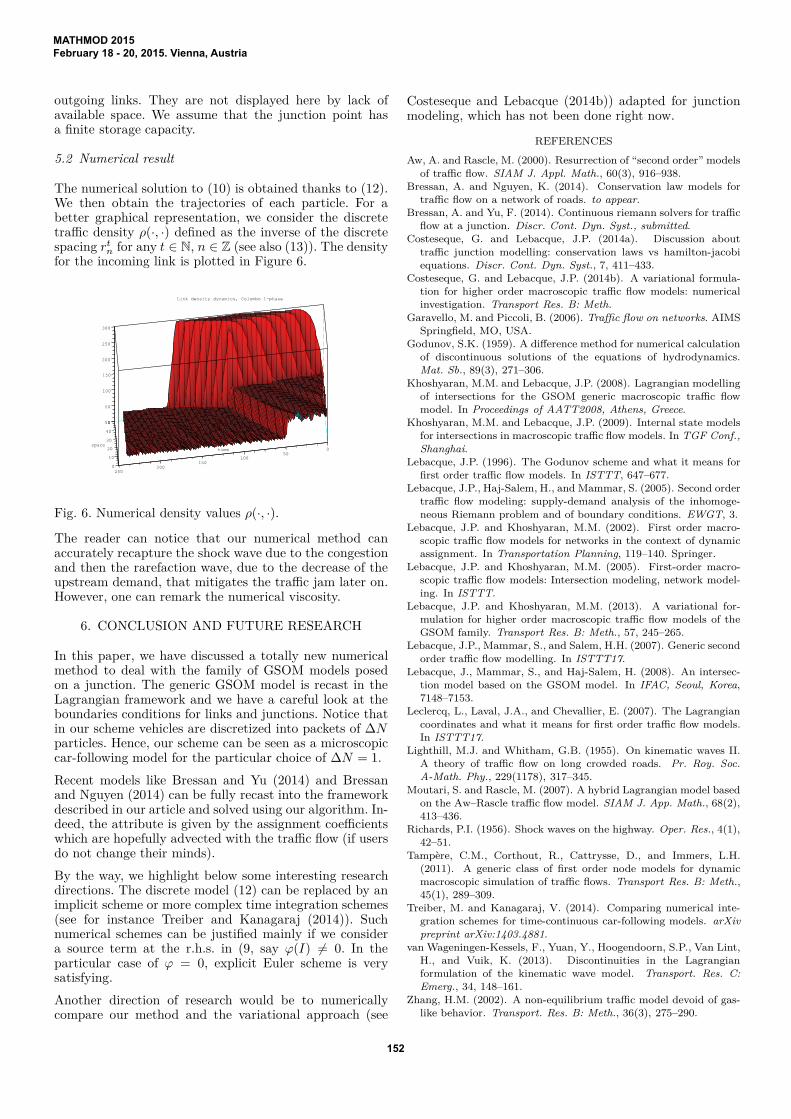
5.2 Numerical result

The numerical solution to (10) is obtained thanks to (12).We then obtain the trajectories of each particle. For abetter graphical representation, we consider the discretetraffic density ρ(·, ·) defined as the inverse of the discretespacing rt

n for any t ∈ N, n ∈ Z (see also (13)). The densityfor the incoming link is plotted in Figure 6.

050

40

30space

0time20

5010010

1502000

250

50

100

150

200

250

300

Link density dynamics, Colombo 1-phase

Fig. 6. Numerical density values ρ(·, ·).

The reader can notice that our numerical method canaccurately recapture the shock wave due to the congestionand then the rarefaction wave, due to the decrease of theupstream demand, that mitigates the traffic jam later on.However, one can remark the numerical viscosity.

6. CONCLUSION AND FUTURE RESEARCH

In this paper, we have discussed a totally new numericalmethod to deal with the family of GSOM models posedon a junction. The generic GSOM model is recast in theLagrangian framework and we have a careful look at theboundaries conditions for links and junctions. Notice thatin our scheme vehicles are discretized into packets of ∆Nparticles. Hence, our scheme can be seen as a microscopiccar-following model for the particular choice of ∆N = 1.

Recent models like Bressan and Yu (2014) and Bressanand Nguyen (2014) can be fully recast into the frameworkdescribed in our article and solved using our algorithm. In-deed, the attribute is given by the assignment coefficientswhich are hopefully advected with the traffic flow (if usersdo not change their minds).

By the way, we highlight below some interesting researchdirections. The discrete model (12) can be replaced by animplicit scheme or more complex time integration schemes(see for instance Treiber and Kanagaraj (2014)). Suchnumerical schemes can be justified mainly if we considera source term at the r.h.s. in (9, say ϕ(I) 6= 0. In theparticular case of ϕ = 0, explicit Euler scheme is verysatisfying.

Another direction of research would be to numericallycompare our method and the variational approach (see

Costeseque and Lebacque (2014b)) adapted for junctionmodeling, which has not been done right now.

REFERENCES

Aw, A. and Rascle, M. (2000). Resurrection of “second order” modelsof traffic flow. SIAM J. Appl. Math., 60(3), 916–938.

Bressan, A. and Nguyen, K. (2014). Conservation law models fortraffic flow on a network of roads. to appear.

Bressan, A. and Yu, F. (2014). Continuous riemann solvers for trafficflow at a junction. Discr. Cont. Dyn. Syst., submitted.

Costeseque, G. and Lebacque, J.P. (2014a). Discussion abouttraffic junction modelling: conservation laws vs hamilton-jacobiequations. Discr. Cont. Dyn. Syst., 7, 411–433.

Costeseque, G. and Lebacque, J.P. (2014b). A variational formula-tion for higher order macroscopic traffic flow models: numericalinvestigation. Transport Res. B: Meth.

Garavello, M. and Piccoli, B. (2006). Traffic flow on networks. AIMSSpringfield, MO, USA.

Godunov, S.K. (1959). A difference method for numerical calculationof discontinuous solutions of the equations of hydrodynamics.Mat. Sb., 89(3), 271–306.

Khoshyaran, M.M. and Lebacque, J.P. (2008). Lagrangian modellingof intersections for the GSOM generic macroscopic traffic flowmodel. In Proceedings of AATT2008, Athens, Greece.

Khoshyaran, M.M. and Lebacque, J.P. (2009). Internal state modelsfor intersections in macroscopic traffic flow models. In TGF Conf.,

Shanghai.Lebacque, J.P. (1996). The Godunov scheme and what it means for

first order traffic flow models. In ISTTT, 647–677.Lebacque, J.P., Haj-Salem, H., and Mammar, S. (2005). Second order

traffic flow modeling: supply-demand analysis of the inhomoge-neous Riemann problem and of boundary conditions. EWGT, 3.

Lebacque, J.P. and Khoshyaran, M.M. (2002). First order macro-scopic traffic flow models for networks in the context of dynamicassignment. In Transportation Planning, 119–140. Springer.

Lebacque, J.P. and Khoshyaran, M.M. (2005). First-order macro-scopic traffic flow models: Intersection modeling, network model-ing. In ISTTT.

Lebacque, J.P. and Khoshyaran, M.M. (2013). A variational for-mulation for higher order macroscopic traffic flow models of theGSOM family. Transport Res. B: Meth., 57, 245–265.

Lebacque, J.P., Mammar, S., and Salem, H.H. (2007). Generic secondorder traffic flow modelling. In ISTTT17.

Lebacque, J., Mammar, S., and Haj-Salem, H. (2008). An intersec-tion model based on the GSOM model. In IFAC, Seoul, Korea,7148–7153.

Leclercq, L., Laval, J.A., and Chevallier, E. (2007). The Lagrangiancoordinates and what it means for first order traffic flow models.In ISTTT17.

Lighthill, M.J. and Whitham, G.B. (1955). On kinematic waves II.A theory of traffic flow on long crowded roads. Pr. Roy. Soc.

A-Math. Phy., 229(1178), 317–345.Moutari, S. and Rascle, M. (2007). A hybrid Lagrangian model based

on the Aw–Rascle traffic flow model. SIAM J. App. Math., 68(2),413–436.

Richards, P.I. (1956). Shock waves on the highway. Oper. Res., 4(1),42–51.

Tampère, C.M., Corthout, R., Cattrysse, D., and Immers, L.H.(2011). A generic class of first order node models for dynamicmacroscopic simulation of traffic flows. Transport Res. B: Meth.,45(1), 289–309.

Treiber, M. and Kanagaraj, V. (2014). Comparing numerical inte-gration schemes for time-continuous car-following models. arXiv

preprint arXiv:1403.4881.van Wageningen-Kessels, F., Yuan, Y., Hoogendoorn, S.P., Van Lint,

H., and Vuik, K. (2013). Discontinuities in the Lagrangianformulation of the kinematic wave model. Transport. Res. C:

Emerg., 34, 148–161.Zhang, H.M. (2002). A non-equilibrium traffic model devoid of gas-

like behavior. Transport. Res. B: Meth., 36(3), 275–290.

MATHMOD 2015February 18 - 20, 2015. Vienna, Austria

152