lagrangian relaxation based decompositon for well...
TRANSCRIPT

Lagrangian Relaxation Based Decompositon for Well Schedulingin Shale-gas Systems
Brage Rugstad Knudsena,∗, Ignacio E. Grossmannb, Bjarne Fossa, Andrew R. Connc
aDepartment of Engineering Cybernetics, Norwegian University of Science and Technology, Trondheim, Norway.bDepartment of Chemical Engineering,Carnegie Mellon University, Pittsburgh, PA 15213, USA.
cIBM T. J. Watson Research Center, Yorktown Heights, NY, USA.
Abstract
Suppressing the effects of liquid loading is a key issue for efficient utilization of mid and late-lifewells in shale-gas systems. This state of the wells can be prevented by performing short shut-inswhen the gas rate falls below the minimum rate needed to avoid liquid loading. In this paper, wepresent a Lagrangian relaxation based scheme for shut-in scheduling of distributed shale multi-well systems. The scheme optimizes shut-in times and a reference rate for each multi-well pad,such that the total produced rate tracks a given short-term gas demand for the field. By usingsimple, frequency-tuned well proxy models, we obtain a compact mixed integer formulationwhich by Lagrangian relaxation renders a decomposable structure. A set of computational testsdemonstrates the merits of the proposed scheme. This study indicates that the method is capa-ble of solving large field-wide scheduling problems by producing good solutions in reasonablecomputation times.
Keywords:Shale-gas production, Lagrangian relaxation, mixed-integer programming, parameterestimation.
1. Introduction
The use of shale-gas as an energy resource has increased extensively over the last decade [1].Even though shale-gas recovery has primarily been a U.S. driven industry, there is currently anincreasing exploration of shale and other tight formation resources both in the Middle East, in theNorth Africa, in China as well as in Europe [2]. The long horizontal wells and stimulation withhydraulic fracturing needed to obtain profitable recovery rates from the very tight rock forma-tions, is however very costly. The last years’ low gas prices have therefore made many shale-gasfields barely economical. This clearly increases the need for efficient planning, exploration andproduction techniques in shale-gas recovery.
Modern shale-gas developments are characterized by an increasing use of multi-well padsfor shearing of surface infrastructure, both in the production from the wells and during the com-pletion [3]. Multi-well pads consist of several wells drilled at a single location, hence reducing
∗Corresponding authorEmail address: [email protected] (Brage Rugstad Knudsen)
Preprint submitted to Elsevier July 5, 2013
Well 1
Well 2
Well j
Multi-well pad
Pipelinenetworks
Multi-well pad l
Multi-well padCompressor/processing station
qPad1
qPad2
qPad3
Total produced gas
Assigned totalreference rate qREF
∑
l∈LqPadl
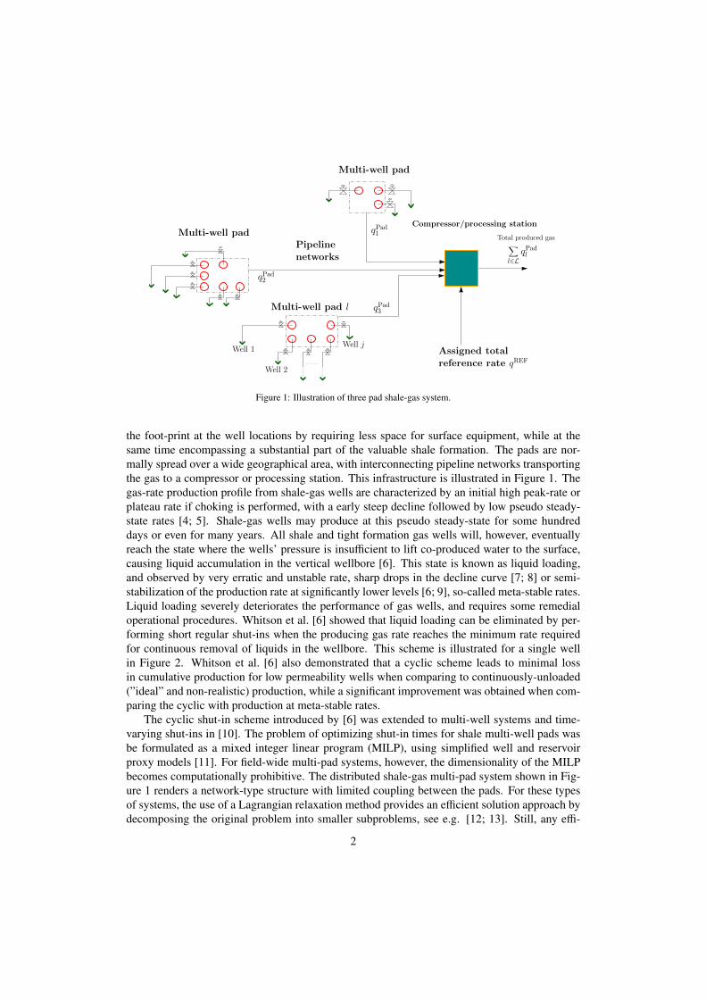
Figure 1: Illustration of three pad shale-gas system.
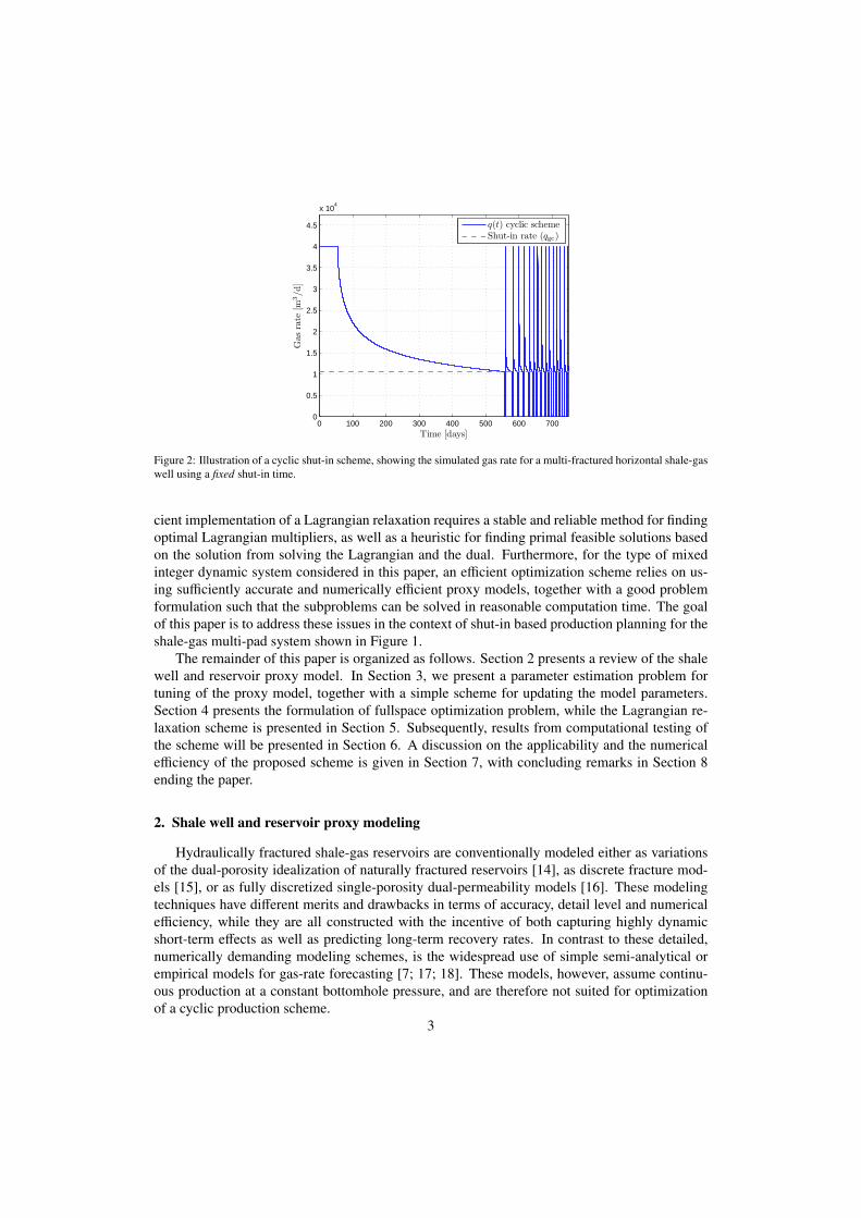
the foot-print at the well locations by requiring less space for surface equipment, while at thesame time encompassing a substantial part of the valuable shale formation. The pads are nor-mally spread over a wide geographical area, with interconnecting pipeline networks transportingthe gas to a compressor or processing station. This infrastructure is illustrated in Figure 1. Thegas-rate production profile from shale-gas wells are characterized by an initial high peak-rate orplateau rate if choking is performed, with a early steep decline followed by low pseudo steady-state rates [4; 5]. Shale-gas wells may produce at this pseudo steady-state for some hundreddays or even for many years. All shale and tight formation gas wells will, however, eventuallyreach the state where the wells’ pressure is insufficient to lift co-produced water to the surface,causing liquid accumulation in the vertical wellbore [6]. This state is known as liquid loading,and observed by very erratic and unstable rate, sharp drops in the decline curve [7; 8] or semi-stabilization of the production rate at significantly lower levels [6; 9], so-called meta-stable rates.Liquid loading severely deteriorates the performance of gas wells, and requires some remedialoperational procedures. Whitson et al. [6] showed that liquid loading can be eliminated by per-forming short regular shut-ins when the producing gas rate reaches the minimum rate requiredfor continuous removal of liquids in the wellbore. This scheme is illustrated for a single wellin Figure 2. Whitson et al. [6] also demonstrated that a cyclic scheme leads to minimal lossin cumulative production for low permeability wells when comparing to continuously-unloaded(”ideal” and non-realistic) production, while a significant improvement was obtained when com-paring the cyclic with production at meta-stable rates.
The cyclic shut-in scheme introduced by [6] was extended to multi-well systems and time-varying shut-ins in [10]. The problem of optimizing shut-in times for shale multi-well pads wasbe formulated as a mixed integer linear program (MILP), using simplified well and reservoirproxy models [11]. For field-wide multi-pad systems, however, the dimensionality of the MILPbecomes computationally prohibitive. The distributed shale-gas multi-pad system shown in Fig-ure 1 renders a network-type structure with limited coupling between the pads. For these typesof systems, the use of a Lagrangian relaxation method provides an efficient solution approach bydecomposing the original problem into smaller subproblems, see e.g. [12; 13]. Still, any effi-
2
0 100 200 300 400 500 600 7000
0.5
1
1.5
2
2.5
3
3.5
4
4.5
x 104
Time [days]
Gas
rate
[m3/d
]
q(t) cyclic schemeShut-in rate (qgc)
Figure 2: Illustration of a cyclic shut-in scheme, showing the simulated gas rate for a multi-fractured horizontal shale-gaswell using a fixed shut-in time.
cient implementation of a Lagrangian relaxation requires a stable and reliable method for findingoptimal Lagrangian multipliers, as well as a heuristic for finding primal feasible solutions basedon the solution from solving the Lagrangian and the dual. Furthermore, for the type of mixedinteger dynamic system considered in this paper, an efficient optimization scheme relies on us-ing sufficiently accurate and numerically efficient proxy models, together with a good problemformulation such that the subproblems can be solved in reasonable computation time. The goalof this paper is to address these issues in the context of shut-in based production planning for theshale-gas multi-pad system shown in Figure 1.
The remainder of this paper is organized as follows. Section 2 presents a review of the shalewell and reservoir proxy model. In Section 3, we present a parameter estimation problem fortuning of the proxy model, together with a simple scheme for updating the model parameters.Section 4 presents the formulation of fullspace optimization problem, while the Lagrangian re-laxation scheme is presented in Section 5. Subsequently, results from computational testing ofthe scheme will be presented in Section 6. A discussion on the applicability and the numericalefficiency of the proposed scheme is given in Section 7, with concluding remarks in Section 8ending the paper.
2. Shale well and reservoir proxy modeling
Hydraulically fractured shale-gas reservoirs are conventionally modeled either as variationsof the dual-porosity idealization of naturally fractured reservoirs [14], as discrete fracture mod-els [15], or as fully discretized single-porosity dual-permeability models [16]. These modelingtechniques have different merits and drawbacks in terms of accuracy, detail level and numericalefficiency, while they are all constructed with the incentive of both capturing highly dynamicshort-term effects as well as predicting long-term recovery rates. In contrast to these detailed,numerically demanding modeling schemes, is the widespread use of simple semi-analytical orempirical models for gas-rate forecasting [7; 17; 18]. These models, however, assume continu-ous production at a constant bottomhole pressure, and are therefore not suited for optimizationof a cyclic production scheme.
3
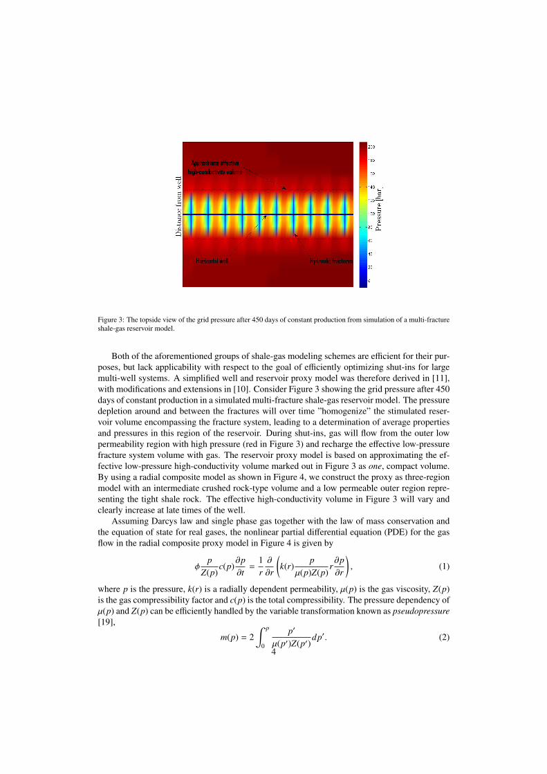
Figure 3: The topside view of the grid pressure after 450 days of constant production from simulation of a multi-fractureshale-gas reservoir model.
Both of the aforementioned groups of shale-gas modeling schemes are efficient for their pur-poses, but lack applicability with respect to the goal of efficiently optimizing shut-ins for largemulti-well systems. A simplified well and reservoir proxy model was therefore derived in [11],with modifications and extensions in [10]. Consider Figure 3 showing the grid pressure after 450days of constant production in a simulated multi-fracture shale-gas reservoir model. The pressuredepletion around and between the fractures will over time ”homogenize” the stimulated reser-voir volume encompassing the fracture system, leading to a determination of average propertiesand pressures in this region of the reservoir. During shut-ins, gas will flow from the outer lowpermeability region with high pressure (red in Figure 3) and recharge the effective low-pressurefracture system volume with gas. The reservoir proxy model is based on approximating the ef-fective low-pressure high-conductivity volume marked out in Figure 3 as one, compact volume.By using a radial composite model as shown in Figure 4, we construct the proxy as three-regionmodel with an intermediate crushed rock-type volume and a low permeable outer region repre-senting the tight shale rock. The effective high-conductivity volume in Figure 3 will vary andclearly increase at late times of the well.
Assuming Darcys law and single phase gas together with the law of mass conservation andthe equation of state for real gases, the nonlinear partial differential equation (PDE) for the gasflow in the radial composite proxy model in Figure 4 is given by
φp
Z(p)c(p)
∂p∂t
=1r∂
∂r
(k(r)
pµ(p)Z(p)
r∂p∂r
), (1)
where p is the pressure, k(r) is a radially dependent permeability, µ(p) is the gas viscosity, Z(p)is the gas compressibility factor and c(p) is the total compressibility. The pressure dependency ofµ(p) and Z(p) can be efficiently handled by the variable transformation known as pseudopressure[19],
m(p) = 2∫ p
0
p′
µ(p′)Z(p′)dp′. (2)
4

kf
re
rwFractured, high-permeability region
Well
km
Horizontal wellbore
Production choke
pw
Intermediate region
Low permeability, nonfractured region
Figure 4: Illustration of proxy model
By using Neumann boundary conditions with a producing well (sink) at the center rw, no-flowconditions at the outer boundary re, and a given initial reservoir pressure, we obtain the followinginitial boundary-value problem (IBVP) in terms of the reservoir pseudopressure m(p) [11].
φµc∂m∂t
=1r∂
∂r
(k(r)r
∂m∂r
), (3a)
r∂m∂r
∣∣∣∣∣rw
= qT psc
Tscπhk, (3b)
∂m∂r
∣∣∣∣∣re
= 0, (3c)
m(r, 0) = minit. (3d)
where q is the gas rate, T is reservoir temperature and h is the horizontal length of the well. Thesubscript sc refers to evaluation at standard condition, 1 bar and 15.6◦C. All gas volumes andvolumetric rates are given in standard conditions in the rest of the paper. The product µc in (3a)is evaluated at given pressures, hence rendering a semi-linear PDE. This technique is elaboratedin Section 3 below. The initial pseudopressure (3d) is calculated by trapezoidal integration of thecorresponding values of p, µ and Z which are obtained by gas correlations, see [20].
The IBVP (3) is discretized in space and time in [11], using a finite difference scheme. Spa-tial discretization applies central difference approximations, i.e. with a second order accuracy.The time discretization uses the backward Euler scheme, or equivalently, a first order orthogonalcollocation on finite elements with fixed element lengths. In the completion and design of shalegas wells, a maximum rate qmax is normally specified based on the surface equipment specifica-tions together with long-term strategic planning of the wells. Moreover, a minimum wellheadpressure is required with respect to the given line pressure. The well rate will initially, or aftera shut-in, deliver a peak or plateau rate for some time until the wellhead pressure is equal to theline pressure and the rate starts to decline. Combing these expected features, a simple aggregatedwell and wellbore model was derived in [11]. Using this aggregated model together with the dis-cretized reservoir proxy model leads to the following simplified single well and reservoir proxy
5

model.
Amk+1 = mk + Bqk+1, (4a)m0 = minit, (4b)
qk = min{qmax, β
(mk1 − m(eS pw)
)}, (4c)
where m ∈ R4 is a vector containing the pseudopressure in each grid block, A is a tridiagonalmatrix, B is a single-column matrix, β is a constant, possibly skin-dependent well index and pwis the wellhead pressure.
2.1. Critical gas rate
A critical gas rate qgc, sometimes referred to as the minimum rate to lift, can be specifiedas a lower bound on the flowing gas rate qk in order to ensure continuous removal of liquidsin the wellbore. The most widely applied model for calculating qgc is given by [21], with theonset of liquid loading observed for the majority of gas wells to be controlled by the wellheadconditions. Coleman, Clay, Mccurdy, and Norris III [22] modified Turner’s criterion for onset ofliquid loading for gas wells with lower wellhead pressures. As shale-gas wells normally operateat low wellhead pressures, we hence use their model for calculating qgc. By ensuring that theproducing gas rate is always greater or equal to qgc, we avoid accumulation of liquids in thevertical part of the wellbore. Furthermore, we limit the valid region of our model and avoid theneed to use a multiphase model for low liquid systems as dry and semi-dry shale-gas wells.
3. Computing model parameters
The gas-rate profile from shale and fractured tight formation wells is observed to be definedby three distinct sets of transients. The first is a steep decline following the early-time peak orplateau rate, during which the gas initially stored in the fracture network is drained. The secondis a very long transient with low rates, often characterized as a pseudo steady-state condition.The last category is pressure build-up transients observable during re-openings of wells aftershut-ins. Modeling all of these transients accurately is recognized as inherently difficult [23],even for very complex and detailed numerical models. Consequently, there are fundamentaltrade-offs when constructing shale-gas models, and clearly a proxy modeling scheme must takeinto account which type of transients the proxy should replicate.
The basis for the scheme we propose is to perform short, regular shut-ins to prevent liq-uid loading. Clearly we are most interested in constructing a model replicating the last of theaforementioned categories of transients, i.e. the transients from re-opening a well after a shut-in. During shut-ins, the gas stored in the low permeable shale matrix will flow into the highlyconductive fractures and refill these small volumes with gas. The transients in the gas rate whenthe well is subsequently started up will exhibit slightly different characteristics depending on thelength of the shut-ins and the pressures at the time of shut-in. The duration of these transientsdepends on the pressure build-up in the near-wellbore region, which in turn depends on severalfactors. The first is the essential reservoir characteristics such as the formation permeability, theconductivity of the fractures and the effective volume of the hydraulically induced and naturalfractures. Some of these properties, in particular the formation permeability and the average frac-ture half-length, can be estimated using the techniques described in [7] and [18]. Other effects
6
that impact the magnitude of the pressure build-up during shut-ins include the total compress-ibility in (3a). Assuming negligible rock compressibility and using the equation of state for realgases, the total compressibility for gas reservoirs under isothermal conditions can be expressedas [20]
c(p) =1ρ
∂ρ
∂p
∣∣∣∣∣T
=1p−
1Z(p)
∂Z(p)∂p
∣∣∣∣∣T. (5)
The compressibility of the gas decreases the initial pressure build-up during shut-ins, as some ofthe pressure change is used to decrease the volume of the gas in pores of the reservoir. Thesepressure effects are strongly nonlinear, and recognized as difficult to include in semi-analyticaland proxy models, particularly in conjunction with the use of pseudopressure m(p). Commonlyapplied techniques include evaluating c(p) at the initial pressure or at the average of the initialreservoir pressure and the bottomhole pressure. Both of the former techniques is equivalent withassuming a slightly compressible fluid. However, instead of choosing at which pressures to eval-uate the compressibility, we parametrize the proxy model (3a) with distinct compressibilities cfand ctran in the fracture region and the transition region, respectively, and apply a tuning of themodel to achieve a good compromise between the compressibility effects during pressure deple-tion and build-up. As the pressure in the outer low permeability region remains almost constant,we evaluate c(p) at initial conditions in this region. We further estimate a fracture radius rf andan approximated well length h for describing the varying effective high-conductivity volume inFigure 3, and an average permeability ktran in the intermediate transition region. Together, thisdefines the vector
θ =[rf ktran cf ctran h
]T(6)
of unknown parameters in the proxy model (4).To estimate parameters in the proxy model, we formulate a constrained weighted nonlin-
ear least squares (WNLS) problem. Using weighted least squares in model tuning and systemidentification as apposed to ordinary LS estimation, provides a means for emphasizing certaindynamics of the system to be modeled. The weighting of the residuals in the WNLS problem canbe obtained by prefiltering of the data [24]. A linear prefilter acts as a frequency weighting of theobjective function, and can be designed to increase the model accuracy in the frequency rangeof interest. This interpretation of the prefilter, however, only applies to strictly linear systemidentification [25]. Moreover, the equivalence of input-output data filtering and prediction errorfiltering in linear LS system identification [24], does in general not hold for nonlinear systems[25]. By using the Volterra series representation of nonlinear systems together with the general-ized frequency response function, Spinelli et al. [25] demonstrated that reduced estimation biasin the desired bandwidth can be achieved by filtering of the prediction errors compared to sep-arate filtering of the input/output data set. Consequently, even though the frequency weightinginterpretation only strictly holds for linear parameter estimation, we can obtain a similar effectin the nonlinear case by filtering the prediction errors through a properly designed filter. Let theprefilter Lp(γ) be given by a general infinite impulse-response filter (IIR),
Lp(γ) =C(γ)D(γ)
=
M1∑m1=0
cm1γ−m1
1 +M2∑
m2=1dm2γ
−m2
, (7)
7
where γ−1 is the unit delay operator1. The filter (7) can be included as a recursive digital filterin the WNLS. Note that the filter equations then simply amounts to a set of linear constraintsenforced for each timestep, and hence do not increase the complexity of the resulting NLP. Weuse a second-order digital low-pass Butterworth filter with a bandwidth [0, 0.4], normalized withrespect to the Nyquist frequency. Let
εk := qk − qMFRk (8)
be the prediction error, where qMFR is the gas rate from the multi-fracture reference model (MFR).Further, let y =
[y1 y2...
]T be a predefined vector of binary valve-settings defining a shut-inschedule. Using an estimation horizon K , we then estimate the proxy model parameters θ bysolving the NLP
minθ
∑k∈K
(εf
k
)2(9a)
s.t.
εfk = Lp(γ)εk ∀k ∈ {K : k ≥ max(M1,M2)} (9b)
εk = qk − qMFRk ∀k ∈ K (9c)
A(θ) mk+1 = mk + B(θ)qk+1, ∀k ∈ K \ K (9d)m0 = minit, (9e)
qk =12
(qk + qmax −
√(qk − qmax)2 + δ2
1 + δ2
), ∀k ∈ K (9f)
qk = yk β(θ)(mk1 − m
(eS pw
)), ∀k ∈ K (9g)
θlo ≤ θ ≤ θup (9h)ctran ≤ cf (9i)
where (9f) is a smooth approximation of the non-smooth well model (4c), with smoothingparameters δ1 and δ2 selected from the interval
[10−2, 10−3
]. The second smoothing parameter
δ2 is added to prevent negative rates when the well is shut-in. Observe that whenever yk = 0for some k ∈ K , then qk = 0 and hence qk ≈ 0 since (9f) gives the minimum of q and qmax.The constraint (9i) is based on the property that average compressibility in the reservoir is highercloser to the wellbore, and serves as a regularization of the parameter estimation problem inaddition to the bounds (9h) [26; 27]. Note that the compact parameteric representation (9d) ofthe discretized PDE model consists of a set of nonlinear equations used to define the spatialgridding and the transmissibilities in the reservoir model. For further details on the derivation ofthe proxy model (9d), see [11].
For the tuning of the proxy model, we use a high-fidelity multi-fracture reference modelconstructed with cylindrical geometry similar to Figure 3 with ten equally spaced fractures. Thehigh-fidelity model is implemented in the state-of-the-art simulation software SENSOR [28],using logarithmic grid refinements between and outside the fractures, with totally 4200 gridcells. We further extend the high-fidelity reservoir model with a static wellbore model, see e.g.
1The unit delay operator is usually defined as q−1 [24]. However, as q is used as notation for the gas rate, we use fornotational convenience γ−1as the equivalent operator.
8
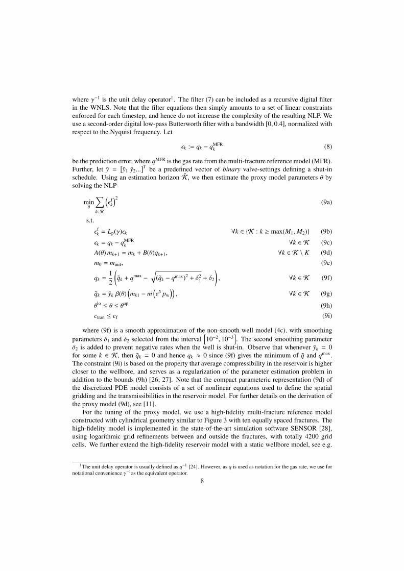
[29]. Essential given model parameters in the proxy and the reference model are quoted in Table1. We use a ∆k = 1 day fixed timestep for the proxy model, while we use a one hour timestepfor the multi-fracture reference model to capture more of the high-frequency dynamics in thismodel. Note that in practice the rates are likely to be available on a daily basis only. The NLP(9) is implemented in GAMS [30] and solved with the NLP solver CONOPT v3.15. The resultsof the tuning of the proxy model is shown in Figure 5, where we have used two shut-ins of fiveand three days, respectively, to excite the model. The proposed modeling and tuning schemerenders a good match of transients after shut-ins of a couple of days. The match is observed tobe tighter in the pseudo-steady state region for the second transient compared to transient afterthe first (five-day) shut-in, while a discrepancy is seen in the peak-rate after the second, three-day long shut-in. This discrepancy reflects the trade-offs made in the proxy modeling (4) and inthe design of the prefilter (7): increasing the bandwidth or shifting the bandpass would increasethe gain on the fast modes of the system and hence, give a better match of the second peak inFigure 5. A nonzero steady-state gain is necessary however to obtain an acceptable match of themodels at the time at which the rates crossed qgc, as the rate at 585 days are almost steady-state.Arguably, one could consider using a bandpass filter instead of a low-pass filter to place moreemphasis on the transient modes and thereby better match the peak rates. This will, however,give a higher bias in the rate of the proxy model in the pseudo steady-state regions, and lead toan almost non-decreasing rate after the initial decline of the rate. Some of the mismatch in thecurvature of the transients is also due to the constant compressibility assumption, while parts ofthe mismatch may be compensated for by a higher-order discretization scheme. Note that theparameter estimate will be somewhat sensitive to the NLP starting point since the WLNS (9) isa non-convex NLP. To compensate for this dependency, we have used a multi start-point strategywith different initial choices θinit to provide good starting points for the NLP (9).
The advantage of using a Butterworth filter is the flat magnitude in the bandpass. However,as Butterworth filters are all-pole filters, there will be a significant phase shift at the output of thefilter, particularly for high-order filters. Care must therefore be taken with respect to the choiceof filter order if the length of the time-series of production rates is short and there are shut-insat the end of time-series, as parts of the transient may be lost due to the phase lag of the filter.Compared to linear system identification, in which a prefilter tends to cut off model content infrequencies outside the bandpass, the prefilter applied in nonlinear system identification intro-duces a scattering of the frequency spectrum outside the bandpass. This property may impact thefrequency weighting in (9) and hence the model match. See [25] for further details and analysis.
Table 1: Given reservoir model parameters.
Symbol Parameter Value Unitφ porosity 6 %km formation permeability 3 × 10⁻⁴ mDzw true vertical depth 2300 mpr initial reservoir pressure 200 barpw minimum wellhead pressure 6.9 barqmax maximum rate 4 × 10⁴ m3/dh true length of horizontal wellbore 492 mnf true number of hydraulic fractures 10 -
9

560 565 570 575 580 5850
0.5
1
1.5
2
2.5
3
3.5
4
4.5
x 104
Time [days]
Gas
rate
[m3/d
]
Proxy modelMulti-fracture reference modelqgc
Figure 5: Tuning of parameters θ the proxy model. The first transient corresponds to a five-day shut-in, while the secondshut-in is three days long.
3.1. Updating model parametersOne of the key issues for industrial appreciation of model-based decision support tools is the
user’s ability to maintain and update the models used [31]. This is particularly challenging forasset and field-wide optimization similar to the problem in this paper, which includes multipledisaggregated model types such as reservoir, surface and wells models, all having different timescales. Challenges are related to the complexity of the models used in the optimization [32], thelevel of automation of the model update, and the (possibly excessive) amount of data available.Quite commonly, models are updated quite infrequently, e.g. on a yearly basis [31]. Such sel-dom model updates introduce a significant time-delay in the feedback decision loop, and clearlydeteriorate the accuracy and the performance of the decision support tool [31]. In this context,there is an evident advantage of using model predictive control (MPC) compared to real-timeoptimization with separate model updating, as model errors and slowly drifting in parameters arecompensated for by the per-timestep feedback and estimation of initial conditions. However, theuse of MPC in a large, geographically spread petroleum production system introduces severalchallenges, and requires a high level of automatic control and less human-in-the-loop operations.
Although a cross-validation in [10] of a similar realization of the proxy model (4) showeda good match with the reference model, the accuracy of the proxy model will abate over time.This is a results of the tuning technique (9d) in which only a limited window of data and shut-insis used, as well as the prefilter. On a long horizon, though, the actual flow and pressure char-acteristics of the reservoir change as result of local pressure depletion in the fracture network,transition to boundary dominated flow and change in proppant distribution and near-wellboreskin [18]. Shale-gas reservoirs may also contain time-varying parameters such as pressure de-pendent formation permeability [16]. The parameter vector θ should hence be updated using amoving horizon-type (MHE) parameter estimation technique [33]. Using a window length Kuof only the last set of applied shut-ins, we limit the weight on the earlier observed shut-ins and
10
tuning of the proxy model. For a given θ∗ obtained by solving the initial parameter estimation(9) shown in Fig. 5, we update the proxy model by solving an augmented form of the WNLSproblem (9),
minθ
∑k∈Ku
(εf
k
)2+ (θ − θ∗)T DT
s PDs (θ − θ∗) (10a)
s.t.equation (9b) - (9i), (10b)
where P is a symmetric positive definite matrix, and Ds is a diagonal scaling matrix used tonormalize the different parameters in θ. The updating of the proxy model by solving (10) isqualitatively different from ordinary moving horizon based parameter (and state) estimation [33].In MHE, the quadratic term in (10a) corresponds to an arrival cost on new data, where an optimalP can be computed by an Extended Kalman filter or other techniques. Consequently, P is in thiscase used to aggregate previously obtained information on the model. The shale-well proxymodel, however, is only valid in a limit area (i.e. over a certain time and pressure range). Ratherthan aggregating information, we want the estimates to be gradually forgotten as new shut-indata becomes available. Consequently, we update the matrix P as a type of forgetting factor [24],
Pk+1 = αIPk (11)
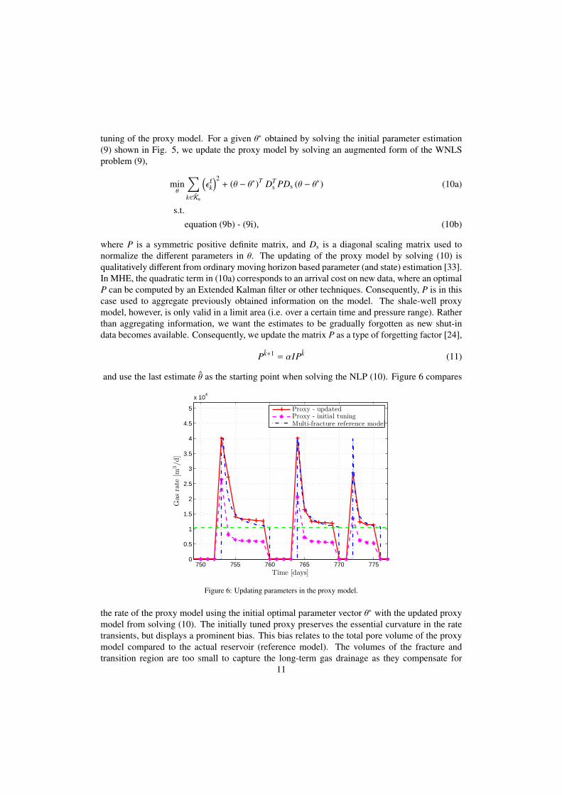
and use the last estimate θ as the starting point when solving the NLP (10). Figure 6 compares
750 755 760 765 770 7750
0.5
1
1.5
2
2.5
3
3.5
4
4.5
5
x 104
Time [days]
Gas
rate
[m3/d
]
Proxy - updatedProxy - initial tuningMulti-fracture reference model
Figure 6: Updating parameters in the proxy model.
the rate of the proxy model using the initial optimal parameter vector θ∗ with the updated proxymodel from solving (10). The initially tuned proxy preserves the essential curvature in the ratetransients, but displays a prominent bias. This bias relates to the total pore volume of the proxymodel compared to the actual reservoir (reference model). The volumes of the fracture andtransition region are too small to capture the long-term gas drainage as they compensate for
11
short-term pressure transients during shut-ins, hence leading to a fast pressure depletion. Theouter, low permeability grid block, which in a way acts as a source term, is unable to compensatefor this pressure depletion, hence leading to high pressure gradients. Figure 6 also shows thedifficulty encountered when shorter shut-ins are used to update the proxy as seen after 772 days.For such short shut-ins the dynamics are even faster, and the proxy does not match the high peakafter re-opening the well.
4. Formulation of optimization problem
Table 2: Indices and set definitions
Index Interpretation Set Elementsi spatial reservoir grid block I {1 . . . I}j well number J {1 . . . J}k discrete time index K {0 . . .K}l pad number L {1 . . . L}n iteration in Lagrangian scheme - {1 . . .N}d terms in the disjunctions - {1, 2, 11, 12, 13}
This section describes the formulation of the optimization problem for the shale-gas multi-pad structure depicted in Figure 1. We assume that a production plan for K days in terms of areference rate qREF is given from strategic and contract based management of the field. Withoutloss of generality, we will assume that the reference rate is constant for the entire horizon K .When shutting in multiple wells at a single location without some scheduling, then in the worstcase the entire set of wells at one pad may be shut in at the same time giving zero total rate,while the peak rate when the wells are subsequently re-opened may be unfeasibly high. Thismust clearly be avoided. We want each pad l ∈ L to produce a stabilized rate qref
l to prevent highpressure and rate oscillations in the feed to the compressors, while at the same time, produceclose to the overall reference rate qREF over the given planning horizon.
Optimization problems with logical structures and conditions may benefit from starting witha generalized disjunctive programming (GDP) formulation [34] instead of an ad-hoc mixed inte-ger formulation, as a GDP formulation generally captures more directly the connections betweenthe logical part and the constraints of the problem [35]. Based on a nonconvex and nonsmoothGDP formulation using the well model (4c) explicitly in the disjunction, an MILP reformula-tion of the problem was derived in [10]. The reformulation is based on a direct big-M typereformulation of the disjunction with an subsequent exact reformulation of the min-function, andwas shown to be computationally superior to equivalent reformulations of the disjunction withsmooth approximations of the min-function. The min-function, however, is a disjunction itself[36]. Consequently, we can rewrite the nonsmooth well-model (4c) as a disjunction based on thewell inflow model and the maximum rate qmax. This disjunction is then embedded into the maindisjunction deciding if a well is producing or shut in. We further include logical constraints forrequiring a minimum shut-in and production time between each succeeding shut-in cycle [10].By combing the reference rate objectives described in the previous paragraph with the logical
12

formulation for shutting in the wells, we obtain the GDP model
Z = min∑l∈L
maxk
∣∣∣qrefl − qPad
lk
∣∣∣ (12a)
s.t. ∑l∈L
qrefl = qREF (12b)
qpadlk =
∑j∈J
q jk, ∀l ∈ L,∀k ∈ K (12c)
Al jml jk+1 = ml jk + Bl jql jk+1, ∀l ∈ L,∀ j ∈ J , k ∈ K \ K (12d)
ml j0 = minitl j , ∀l ∈ L,∀ j ∈ J (12e)
ql jk = β j
(ml jk1 − m
(eS l j pw,l j
)), ∀l ∈ L,∀ j ∈ J ,∀k ∈ K (12f)
Y1l jk
ql jk ≥ qgcY11
l jkql jk ≤ qmax − δe
ql jk = ql jk
∨
Y12l jk
ql jk ≥ qmax
ql jk = qmax
∨
[Y2
l jkql jk ≡ 0
], ∀l ∈ L,∀ j ∈ J , k ∈ K (12g)
Y1l jk Y Y2
l jk, ∀l ∈ L,∀ j ∈ J , k ∈ K (12h)
Y1l jk ⇔ Y11
l jk Y Y12l jk, ∀l ∈ L,∀ j ∈ J , k ∈ K (12i)(
Y1l jk−1 ∧ ¬Y2
l jk
)⇒ Y2
l jk+1 ∧ . . . ∧ Y2l jk+τ1−1, ∀l ∈ L,∀ j ∈ J , k ∈ {K : 1 ≤ k ≤ K − τ1 + 1}
(12j)(Y1
l jk ∧ Y2l jk−1
)⇒ Y1
l jk+1 ∧ . . . ∧ Y1l jk+τ2−1, ∀l ∈ L,∀ j ∈ J , k ∈ {K : 1 ≤ k ≤ K − τ2 + 1}
(12k)
Y1l jk,Y
11l jk,Y
12l jk,Y
2l jk ∈ {True, False}
Observe that in (12a) we have used the sum of the infinity norm between the per timestep pad rateqpad
lk and the corresponding pad reference rate qrefl as the objective function. The constant δe in
(12g) is included to enforce non-satisfaction of both of the terms in the embedded disjunctions,and is set typically to 0.001 in implementations (cf. [37]). The above logic-based problemformulation is in non-standard GDP form [34; 35] due to the embedded disjunction (12g), butcan be systematically transformed into standard GDP form by using the technique described
13

[35; 37]. This leads to the following logically equivalent representation of the disjunction (12g),[Y1
l jkql jk ≥ qgc
]∨
[Y2
l jkql jk = 0
], ∀l ∈ L,∀ j ∈ J , k ∈ K (13a)
Y11l jk
ql jk ≤ qmax − δe
ql jk = ql jk
∨
Y12l jk
ql jk ≥ qmax
ql jk = qmax
∨ [Y13
l jk
], ∀l ∈ L,∀ j ∈ J , k ∈ K (13b)
Y1l jk Y Y2
l jk, ∀l ∈ L,∀ j ∈ J , k ∈ K (13c)
Y11l jk Y Y12
l jk Y Y13l jk, ∀l ∈ L,∀ j ∈ J , k ∈ K (13d)
Y1l jk ⇔ Y11
l jk Y Y12l jk, ∀l ∈ L,∀ j ∈ J , k ∈ K (13e)
Y13l jk ⇔ Y2
l jk. ∀l ∈ L,∀ j ∈ J , k ∈ K (13f)
The Boolean Y13 is introduced to allow the logical state ¬Y11 ∧ ¬Y12. Transforming (12) intothe standard form (13) allows us to asses different ways of reformulating the disjunctions intoalgebraic equations. Raman and Grossmann [34] showed how linear GDPs can be convertedto MILPs by introducing binary variables y with one-to-one correspondence with the Booleanvariables Y , and using either a Big-M reformulation [36] or the convex hull description of gen-eral linear disjunctions derived by Balas [38]. The polyhedral convex hull description of lineardisjunctions is based on disaggregation of the variables in the disjunction and assuring that onlyone of the terms in the disjunction is active. The convex hull reformulation yields an LP relax-ation at least as tight or tighter than big-M reformulations, and hence generally stronger lowerbounds and reduced computation time [35; 39]. Still, the convex hull reformulation requires morevariables and constraints than big-M reformulations. This may translate into longer computationtime for some problems [35; 39]. Based on our computational experience, we observed that a fullconvex hull reformulation of the disjunctions (13a)–(13b) resulted in longer computation timesthan using the convex hull reformulation for (13a) and a big-M reformulation of (13b), whileonly a marginal improvement in the LP relaxation was observed when using the full convex hullreformulation. Disaggregation of ql jk in (13a) then yields
ql jk = q1l jk + q2
l jk, ∀l ∈ L,∀ j ∈ J , k ∈ K (14)
y1l jk + y2
l jk = 1, ∀l ∈ L,∀ j ∈ J , k ∈ K (15)
q1l jk, q
2l jk ≥ 0, (16)
which by substitution of the disaggregated variables into (13a) simplifies to
qgcy1l jk ≤ ql jk ≤ y1
l jkqmax, ∀l ∈ L,∀ j ∈ J , k ∈ K (17)
since q2l jk ≡ 0, and ql jk does not appear in this disjunction. The big-M reformulation of (13b) is
obtained by rewriting the equality constraints as two inequalities and introducing big-M param-eters for each term. The logical proposition (12j)–(12k) for the minimum shut-in and productiontime can be transformed to linear algebraic inequalities by replacing the implications with dis-junctions, converting the resulting disjunction to conjunctive normal form and then replacing thelogical relations with its algebraic counterparts, see [40]. This eventually leads to the followingprimal MILP problem.
14

Z = min∑l∈L
fl (18a)
s.t.
qREF =∑l∈L
qrefl (18b)
fl ≥ qrefl − qpad
lk , ∀l ∈ L, k ∈ K (18c)
fl ≥ −qrefl + qpad
lk , ∀l ∈ L, k ∈ K (18d)
qPadlk =
∑j∈J
q jk, ∀l ∈ L,∀k ∈ K (18e)
Al jml jk+1 = ml jk + Bl jql jk+1, ∀l ∈ L,∀ j ∈ J , k ∈ K \ K (18f)ml j0 = minit, ∀l ∈ L,∀ j ∈ J (18g)
ql jk = β j
(ml jk1 − m
(eS l j pw,l j
)), ∀l ∈ L,∀ j ∈ J ,∀k ∈ K (18h)
qgcy1l jk ≤ ql jk, ∀l ∈ L,∀ j ∈ J , k ∈ K (18i)
ql jk ≤ qmaxy1l jk, ∀l ∈ L,∀ j ∈ J , k ∈ K (18j)
ql jk − qmax + δe ≤ M11(1 − y11
l jk
), ∀l ∈ L,∀ j ∈ J , k ∈ K (18k)
ql jk − ql jk ≤ M11(1 − y11
l jk
), ∀l ∈ L,∀ j ∈ J , k ∈ K (18l)
ql jk − ql jk ≤ M11(1 − y11
l jk
), ∀l ∈ L,∀ j ∈ J , k ∈ K (18m)
qmax − ql jk ≤ M12(1 − y12
l jk
), ∀l ∈ L,∀ j ∈ J , k ∈ K (18n)
ql jk − qmax ≤ M12(1 − y12
l jk
), ∀l ∈ L,∀ j ∈ J , k ∈ K (18o)
qmax − ql jk ≤ M12(1 − y12
l jk
), ∀l ∈ L,∀ j ∈ J , k ∈ K (18p)
y11l jk + y12
l jk + y13l jk = 1 ∀l ∈ L,∀ j ∈ J , k ∈ K (18q)
y11l jk + y12
l jk = y1l jk ∀l ∈ L,∀ j ∈ J , k ∈ K (18r)
y1l jk + y2
l jk = 1 ∀l ∈ L,∀ j ∈ J , k ∈ K (18s)
y13l jk = y2
l jk ∀l ∈ L,∀ j ∈ J , k ∈ K (18t)
y1l jk−1 + y2
l jk ≤ 1 + y2l jρ, ∀l ∈ L,∀ j ∈ J , k ∈ K \ 0 (18u)
ρ ∈ [k + 1,min {k + τ1 − 1,K}] (18v)
y2l jk−1 + y1
l jk−1 ≤ 1 + y1l jρ, ∀l ∈ L,∀ j ∈ J , k ∈ K \ 0 (18w)
ρ ∈ [k + 1,min {k + τ2 − 1,K}] (18x)
Introducing the auxiliary variables fl with the constraints (18c)–(18d) exactly reformulates thenon-smooth objective function (12a). Note that although the MILP formulation (18) can beconsiderably reduced by substituting dependent binary variables, we leave this reduction andtightening of the problem to the presolve routines in the MILP solver (such as CPLEX andGurobi).
Similar constraints as (18u)–(18w) for the minimum shut-in and production time for each15
shut-in cycle have been used for defining minimum up and down time requirements in the hydro-thermal unit commitment (UC) problem in power generation [41], as well as restricted lengthset-up sequences in single-item lot sizing [42]. Several authors have studied the tightness ofdifferent formulations of these constraints in the context of the UC problem [43; 44]. Rajanand Takriti [44] derives the convex hull polytope of an extended variable formulation of theminimum up and downtime constraints, in which start-up and shut-down costs are present. Asthe problem (12) contains no costs on the shut-ins and start-ups, however, we can omit additionalbinary variables for modeling start-up and shut-ins transitions, and limit the formulation of theminimum shut-in and production time constraints using only the on/off variables y1
l jk and y2l jk
with the constraints (18u)–(18w). Note that these constraints are projections of the so-called turnon/off inequalities derived in [44] onto the space of the y1
l jk and y2l jk variables [42].
5. Lagrangian relaxation scheme
Lagrangian relaxation is an efficient solution technique for problems with a block-separablestructure in the constraint set and few binding or coupling constraints. This structure is oftenfound in optimization problems with some sort of network flow and spatial distribution [12; 13].The primal problem (18) clearly renders this type of problem structure, as the only constraintthat links the L pads together is the constraint (18b) requiring that the sum of the individualpad reference rates must equal the total requested rate qREF. Consequently, by dualizing thisconstraint, we will obtain a block-separable, decomposable problem with one subproblem foreach pad l ∈ L. Let λ ∈ R be the Lagrangian multiplier associated with the reference rateequality constraint (18b). The Lagrangian relaxation is then given by
ZLR(λ) = min∑l∈L
fl + λ
∑l∈L
qrefl − qREF
(19)
s.t.eq. (18c)–(18w),
hence rendering a spatial decomposition over the set L, such that solving the Lagrangian (19)means solving l independent subproblems defined by
ZlLR = min fl + λqref
l (20)s.t.
eq. (18c)–(18w) for given l ∈ L.
For any λ ∈ R, the Lagrangian (19) is a relaxation of the primal problem (18), and consequentlydefines a lower bound on Z [45; 46]. The solution of the Lagrangian (19) yields a lower boundon Z as least as tight as the LP relaxation [45]. The dual variable λ is a marginal cost on thedemand constraint (18b) of the pads’ reference rate qref
l relative to the given total reference rate(or demand) qREF, by pricing the cost of satisfying an additional unit in total gas demand [13].
Obtaining the best possible value ZLR(λ) of the Lagrangian relaxation (19), that is, the oneproviding the tightest lower bound on Z, requires finding the optimal multiplier λ. This problemdefines the Lagrangian Dual [45],
ZD = maxλ
ZLR(λ). (21)
16
The Lagrangian ZLR(λ) can be shown to be concave and piecewise linear, and hence nonsmooth[36]. Solving (21) hence requires using techniques for nonsmooth optimization. The solutionof (21) will in most cases be primal infeasible in the sense that the dualized reference rate con-straint (18b) will be violated. Consequently, some technique using the information from solvingthe Lagrangian relaxation and/or the Lagrangian dual must be developed for generating primalfeasible solutions.
5.1. Solving the Lagrangian DualThe two most common classes of algorithms for solving the Lagrangian duals are subgra-
dients methods and methods based on the cutting-plane approach [47]. A variety of implemen-tations and modification of algorithms within these two classes exists. The subgradient-typemethods do not require solution of any optimization problem and are hence easy to implement.They are based on using the dualized constraint, i.e. (18b) in the Lagrangian relaxation (19),as the subgradient for ZLR in the space of the dual variables. Subgradient methods may requireextensive tuning of the stepsize parameters to obtain good practical convergence, and lack atrue termination criteria. By substituting (19) for ZLR in the Lagrangian Dual (21), we obtain amaximin problem, which can be equivalently written a the semi-infinite linear program [48]
ZD = maxλ,η
η (22a)
s.t.
η ≤∑l∈L
fl + λ
∑l∈L
qrefl − qREF
, ( fl, qrefl ) ∈ Q (22b)
where Q is a polytope, by assumption, defining the feasible set of the Lagrangian relaxation, andη ∈ R. The cutting plane method is based on replacing (22b) with a subset of cuts accumulatedby solving the Lagrangian relaxation. This approach renders the linear program
ZD = maxλ,η
η (23a)
s.t.
η ≤∑l∈L
f nl + λ
∑l∈L
qref,nl − qREF
n = 1, 2, ... (23b)
for the Lagrangian Dual, where n is the number of iterations in the primal-dual loop solving (19)and (23). At each step of the loop, solving (23) provides an upper and lower bound on ZD [46],
ηn ≥ ZD ≥ ZnLR (24)
The method terminates when these bounds coincide. The cutting-plane method has finite con-vergence [48], but suffers in its basic form from an inherent instability. In early iterations, thecutting-plane model (23b) of Q is insufficient to provide a bounded problem. Moreover, thesequence λn of dual solutions lack local properties [46]. These characteristics often leads to os-cillatoric performance and slow convergence of the cutting-plane method in practice. The prob-lem of early oscillations and unbounded solutions of (23) can be addressed by adding boundson the dual variables [48], and adding known solutions ( fl, qref
l ) of (18) and (20) to improve thecutting-plane model (23b) of Q [46]. Many rigorous stabilization methods have been suggested
17

to increase the local properties and mitigate the oscicillations of the dual solutions from thecutting-plane method, see [48]-Ch. XV and [46] for a thorough review. The above approachesfor stabilizing the cutting plane method for the Lagrangian Dual may be combined and tailoredto derive efficient algorithms for updating the Lagrangian multipliers, or possibly combined witha subgradient method [49].
To stabilize the cutting-plane formulation for solving the Lagrangian Dual (23), we adopta trust-region scheme from [48] and [50]. The trust-region approach provides a simple devicefor coping with instabilities in the cutting-plane method when applied to Lagrangian Duals withrelatively few dual variables, and is closely related to the boxstep method [51]. The algorithmensures that the next λn+1 is never further away than a distance ∆ from the current stability centerλ. The algorithm is as follows:
Algorithm 1: Trust-region cutting-plane methodInitialization: Select initial trust-region ∆1, stability center λ, a termination tolerance ρCP, and adescent coefficient σ ∈ (0, 1). Set λ1 = λ, N := 1, and solve (19) to obtain ZLR(λ1).
Step 1: Solve the LP
maxλ,η
η (25a)
s.t.
η ≤∑l∈L
f nl + λ
∑l∈L
qref,nl − qREF
, ∀n ≤ N (25b)
|λ − λ| ≤ ∆n (25c)λ ≥ −1 (25d)
to obtain λn+1. Computeρ := η − ZLR(λ) (26)
Step 2: If ρ < ρCP, terminate with λ = λ and ZD = ZLR(λ)
Step 3: Compute ZLR(λn+1).
Step 4: IfZLR(λn+1) ≥ ZLR(λ) + σρ, (27)
update the center: λn+1 = λn+1. Otherwise, leave center unchanged.
Step 5: Update trust-region; compute the ratio
ρ :=ZLR(λn+1) − ZLR(λ)
ρ(28)
If ρ = 1, set ∆n+1 = 1.5∆n. If ρ < 0, set ∆n+1 = 0.8∆n
Set n = n + 1, N = n + 1, and repeat from Step 1.
18
By evaluating in step 4 the ratio of the predicted decrease in the gap ρ with the actual decrease,an ascent-step (serious step) is only declared if a sufficient decrease is obtained relative to theparameter σ. Otherwise, the current iteration is a null-step, while the cutting-plane model (25)is updated. Comparing with the subgradient method, the above scheme guarantees an increasefor each serious step. The numerical value of the Armijo-like parameter σ is set to 0.01. Thetrust-region radius is only updated when λ is on the boundary of the region (cf. [50]). Thisway of updating the radius, together with the trust-region adjustment factors 0.8, 1.5, may betuned to improve the performance of the algorithm. Note that we have used the 1-norm for thetrust-region (25c); for higher dimensional problems, the Euclidean norm may be more suitable,however leading to a nonlinear problem.
The lower bound (25d) is added to ensure values of λ that gives bounded Lagrangian sub-problems (20). The proof of the numerical value of this bound is given in Appendix A. By asimilar proof, it can be shown by using Fourier-Motzkin elimination that for a single referencerate qREF, any non-negative value of λ will cause qref
l = 0, and consequently the optimal solutionfl = qpad
l = 0 for each of the subproblems (20). Hence, we can add this a priori solution to (25) toimprove the initial cutting-plane model of (22). Note that in practice, though, it may be sufficientto select an initially small trust-region ∆ together with a good estimate for λ1 = λ to preventoptimal values of λ less than -1.
5.2. Generating primal feasible solutions
Obtaining primal feasible solutions in a Lagrangian relaxation scheme normally requiresthe use of some, possibly problem specific, heuristic. Either or both of the solutions from theLagrangian relaxation and the Lagrangian Dual may be exploited to generate primal feasible so-lutions, often using some type of greedy algorithm. The solutions from the Lagrangian relaxationoften becomes almost primal feasible (with respect to the dualized constraints) with increasingnumber of iterations. As ZLR is a best-bound on Z, the solution of the Lagrangian relaxation mayin some way aid the search for primal feasible solutions.
Solving the |L| Lagrangian subproblems generates a schedule (or sequence) of shut-ins foreach well on the given pad l together with a reference-rate qref
l . The shut-in schedule is completelydescribed by the value of the binary variables yd
l jk. Consequently, the solution of the subproblemsavoid liquid loading in the wells. On the other hand, the shut-in schedule will be affected by thevalue of the qref
l , which in turn is a function of the marginal cost λ and the total capacity of wellson the pad. That is, how much gas the wells can produce and the level of the peak-rates aftershut-ins. To obtain a primal feasible solution and hence an upper bound ZUB, we fix the binaryvariables yd
l jk to the value obtained from solving the Lagrangian relaxation subproblems (20), andsolve the primal problem (18). This variable fixing then corresponds to fixing the well schedule.The primal problem (18) reduces to an LP, where qref
l now are the only degrees of freedom.The LP solution of this variable fixing returns a set of primal feasible reference rates qref
l whichminimizes (in terms of the sum of the maximum norm) the deviation between the currently fixedproduction and the reference rates .
If the deviation between the primal feasible reference rates qrefl from the binary variable
fixing, and the corresponding solution qrefl from the Lagrangian relaxation is larger than a certain
threshold, ∣∣∣qrefl − qref
l
∣∣∣ > δref, (29)
19

we perform a local search for each of these pads l ∈ L ⊆ L to search for an improved shut-inschedule. Let Zl = fl be the solution from (18a) for pad l obtained by the binary variable fixing.The local search is then performed by fixing the reference rate, qref
l ≡ qrefl , and solving the MILP
problem
Zl = min fl (30a)s.t.
fl ≤ Zl (30b)
fl ≥ qrefl − qpad
lk , k ∈ K (30c)
fl ≥ −qrefl + qpad
lk , k ∈ K (30d)∑(l, j,k)∈
{(L×J×K):y1
l jk=1}(1 − y1
l jk) +∑
(l, j,k)∈{(L×J×K):y2
l jk=1}(1 − y2
l jk) ≤ r, (30e)
eq. (18e)–(18w) for given l ∈ L.
The constraint (30e) is a local branching type constraint [52], where y1l jk, y
2l jk is the shut-in sched-
ule obtained from the solving the Lagrangian relaxation, and the parameter r is a neighborhoodradius (or Hamming distance). This constraint allows at most r switchings of wells from on tooff and from off to on, given by the first and the second term, respectively. The radius r mustbe selected sufficiently large for improved solutions to exist, while at the same time being smallenough such that the local search can be performed numerically efficient. We implement a strat-egy where we initialize r = d(1/3) |K| |J|e, and increase r by 50% a maximum of five times if(30) is infeasible, and we allocate a maximum CPU time between 15-90 seconds for each localsearch, depending on the problem size.
If the loop in Lagrangian scheme terminates with a nonzero duality gap, we perform anextended but similar local search like (30) for the best found feasible solution. In particular, weremove the local branching constraint (30e) and perform a time-limited search, with qref
l nowfixed to the best found primal feasible solution. In contrast, the local search (30) inside theloop is based on the deviation between the currently obtained feasible solution and solution fromthe current iteration of the Lagrangian relaxation. Note that we preserve primal feasibility whenperforming the local search. If the solution improves the upper bound, we update the best feasiblesolution and terminates the scheme.
The complete Lagrangian relaxation scheme is outlined in Figure 7.
6. Computational Results
The performance of the Lagrangian relaxation scheme is assessed by solving a series oftest sets of the shale-gas multi-pad system with the structure shown in Figure 1. The setsare generated with different number of pads |L|, while we for simplicity have used six wellsper pad l. The proxy models in the numerical examples are realized and tuned against themulti-fracture reference model as described in section 3, using three different permeabilitieskm ∈
[1 × 10⁻⁴, 3 × 10⁻⁴, 5 × 10⁻⁴
]. When using equal fracture geometry and initial pressure,
the value of the formation permeability is decisive for the time when the gas rate first crosses thecritical rate qgc, hence giving somewhat different performance of the wells. We assume equalpermeability for each well on given pad, but we will assume that each well have been operated
20

Set max iter N , and tolerances ρCP, σ,
δref , and εd . Set ZUB =∞, n = 1Choose λ,∆1, and set λ = λ1
Solve |L| subproblems tocompute ZLR(λ)
While n ≤ N
ZUB − ZLR(λ) < εd ?
n = n+ 1
1. The Lagrangian relaxation
3. Lagrangian Dual
Initialization
Update λ and ∆.Add cut and solve Lagrangian Dual
to obtain λn+1
η − ZLR(λ) < ρCP ?yes
Terminate
Update ZUB
Perform local search 2.Primalheuristic
yesTerminate
no
no
Fix binary varibles ydljk
Perform local searchto improve ZUB
Termination heuristic
Figure 7: Schematic description of Lagrangian relaxation scheme.
21

different lengths of time, hence giving different initial pseudopressures minitl j . We use a one-day
fixed timestep, and set τ1 = τ2 = 2 days.The entire Lagrangian scheme illustrated in Figure 7 is implemented in GAMS [30], using
IBM CPLEX v12.3 to solve the LPs and the MILPs. The problems are solved using a Dell laptopwith Intel I7 quad-core CPU and 8GB of RAM, using deterministic parallel mode with up to 8threads. The tolerances are set to ρCP = 10−6, σ = 0.01, δref = 0.01 and εd = 0.01, while themaximum number of iteration are set to N = 15. The trust-region is initially set to ∆1 = 0.3and λ = −0.5. For the MILP Lagrangian relaxation subproblems (20), we use a relative gap lessthan 1% or an absolute gap less than 10−4 as stopping criteria, and allocate a maximum CPUtime of four hours for each of the subproblems. The absolute-gap criteria is added as a the LPrelaxation for the subproblems tends to be zero or a very small value, since we are minimizingthe deviation between a reference and the rate. The size of the problems are shown in Table 3.Note that the size of the MILPs are significantly reduced by the presolve routines in CPLEX. Allreported times are real (clock) time, and the reported gaps are defined as [42]
DG := 100[%] ×|ZUB − ZLB|
|ZUB|. (31)
The results of the Lagrangian scheme is compared in Table 4 with the fullspace solution of theprimal MILP model (18). We allocate a solution time for the fullspace solution approximatelyequal to the time spent by the Lagrangian scheme.
Table 3: Problem parameters before reduction in presolve routines
Problem size|L| K Binary var. Cont. var Constraints3 7 720 895 26663 14 1350 1672 51033 21 1980 2449 75806 7 1140 1789 53306 14 2700 3343 102446 21 3960 4897 151589 7 2160 2686 79949 14 4050 5014 153659 21 5940 7345 22736
Table 4 shows characteristics of the results of applying the Lagrangian relaxation scheme tosets with different number of pads and planning horizons. All of the sets in Table 4, except forthe sets with |L| = 6 and K = 14 and 21, respectively, are terminated by the criteria ρ ≤ ρCP instep 2 of the trust-region method for solving the Lagrangian Dual (21). None of the sets reachthe maximum number of iterations. Several of the sets terminate with duality gaps greater than10%. Hence, if only evaluated by size of the duality gap, the performance of the Lagrangianrelaxation scheme applied to these sets may be considered as only average. The final dualitygaps are not necessarily worse for longer compared to short planning horizons K. For planninghorizons longer than three weeks, the time required to solve each of the MILP subproblemsto global optimality becomes computationally prohibitive. The difficulty in solving the MILP(18) becomes evident when comparing the solution characteristics of the Lagrangian schemewith solving the fullspace problem (18) with a global method, that is, a direct approach. The
22
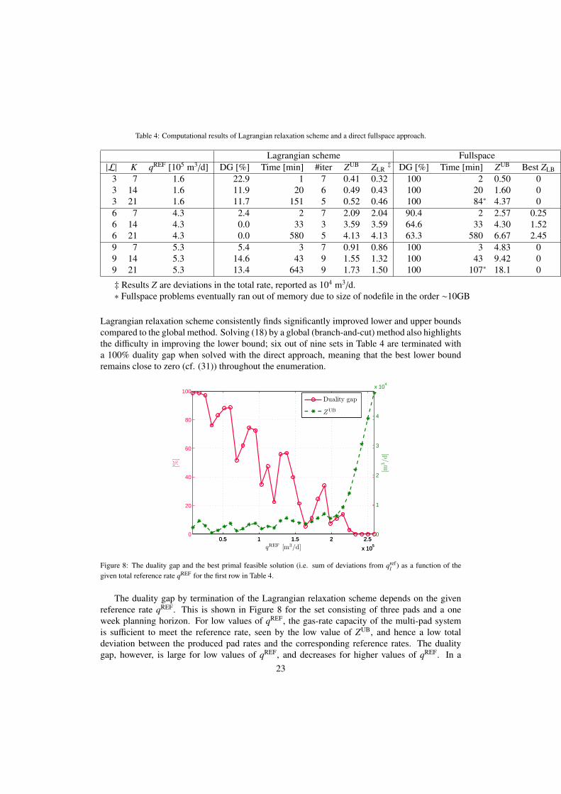
Table 4: Computational results of Lagrangian relaxation scheme and a direct fullspace approach.
Lagrangian scheme Fullspace|L| K qREF [105 m3/d] DG [%] Time [min] #iter ZUB ZLR
‡ DG [%] Time [min] ZUB Best ZLB
3 7 1.6 22.9 1 7 0.41 0.32 100 2 0.50 03 14 1.6 11.9 20 6 0.49 0.43 100 20 1.60 03 21 1.6 11.7 151 5 0.52 0.46 100 84∗ 4.37 06 7 4.3 2.4 2 7 2.09 2.04 90.4 2 2.57 0.256 14 4.3 0.0 33 3 3.59 3.59 64.6 33 4.30 1.526 21 4.3 0.0 580 5 4.13 4.13 63.3 580 6.67 2.459 7 5.3 5.4 3 7 0.91 0.86 100 3 4.83 09 14 5.3 14.6 43 9 1.55 1.32 100 43 9.42 09 21 5.3 13.4 643 9 1.73 1.50 100 107∗ 18.1 0
‡ Results Z are deviations in the total rate, reported as 104 m3/d.∗ Fullspace problems eventually ran out of memory due to size of nodefile in the order ∼10GB
Lagrangian relaxation scheme consistently finds significantly improved lower and upper boundscompared to the global method. Solving (18) by a global (branch-and-cut) method also highlightsthe difficulty in improving the lower bound; six out of nine sets in Table 4 are terminated witha 100% duality gap when solved with the direct approach, meaning that the best lower boundremains close to zero (cf. (31)) throughout the enumeration.
0.5 1 1.5 2 2.5
x 105
0
20
40
60
80
100
[%]
qREF [m3/d]
0.5 1 1.5 2 2.5
x 105
0
1
2
3
4
x 104
[m3/d
]
Duality gap
ZUB
Figure 8: The duality gap and the best primal feasible solution (i.e. sum of deviations from qrefl ) as a function of the
given total reference rate qREF for the first row in Table 4.
The duality gap by termination of the Lagrangian relaxation scheme depends on the givenreference rate qREF. This is shown in Figure 8 for the set consisting of three pads and a oneweek planning horizon. For low values of qREF, the gas-rate capacity of the multi-pad systemis sufficient to meet the reference rate, seen by the low value of ZUB, and hence a low totaldeviation between the produced pad rates and the corresponding reference rates. The dualitygap, however, is large for low values of qREF, and decreases for higher values of qREF. In a
23

certain range of values for qREF, it is seen that the size the duality gap compared the value of ZUB
is balanced. For high values of qREF, the duality gap converges to zero while the optimal solutionvalue increases rapidly, leading to unacceptable deviations between the produced rates and thereference rates.
The trust-region cutting-plane algorithm works well for solving the Lagrangian Dual of theproblem. All sets terminate with an optimal dual variable λ after 4-9 iterations. The methodis also observed to be fairly robust with respect to initial choices of λ and ∆i. Still, choosing ahigher value of the initial trust region and a lower initial value of λ (closer to -1) leads to slightlymore iterations and to increased oscillations in the sequence of solutions λn. In this case thetrust-region becomes ineffective. The use of the local search procedure (30) mainly improvedthe upper bound ZUB whenever the binary-fixing heuristic found an improved primal feasiblesolution. In these cases, however, the local search often reduces the upper bound with 50-200%,relatively.
The practical performance of the solving (18) is illustrated in Figure 9 showing the total ratefor the set in Table 4 with 9 wells and a three week planning horizon. The reference rate andthe total produced rate is shown for three of the nine pads in Figure 10. The total gas rate forthe pads is shown to tightly follow the given total reference rate qREF over the planning horizon,while each of the pads rates follow the optimal pad reference rates with only small fluctuationsas seen in Figure 10. Consequently, any high and low peak rates are avoided, both in the totalrate, and for the rates from the individual pads. In this context, the actual optimized result bythe Lagrangian relaxation scheme clearly renders a good feasible solution despite the dualitygap being more than 13%. Comparing the subfigures in Figure 10 also highlights a qualitativedifference in the performance of the gas rates qpad
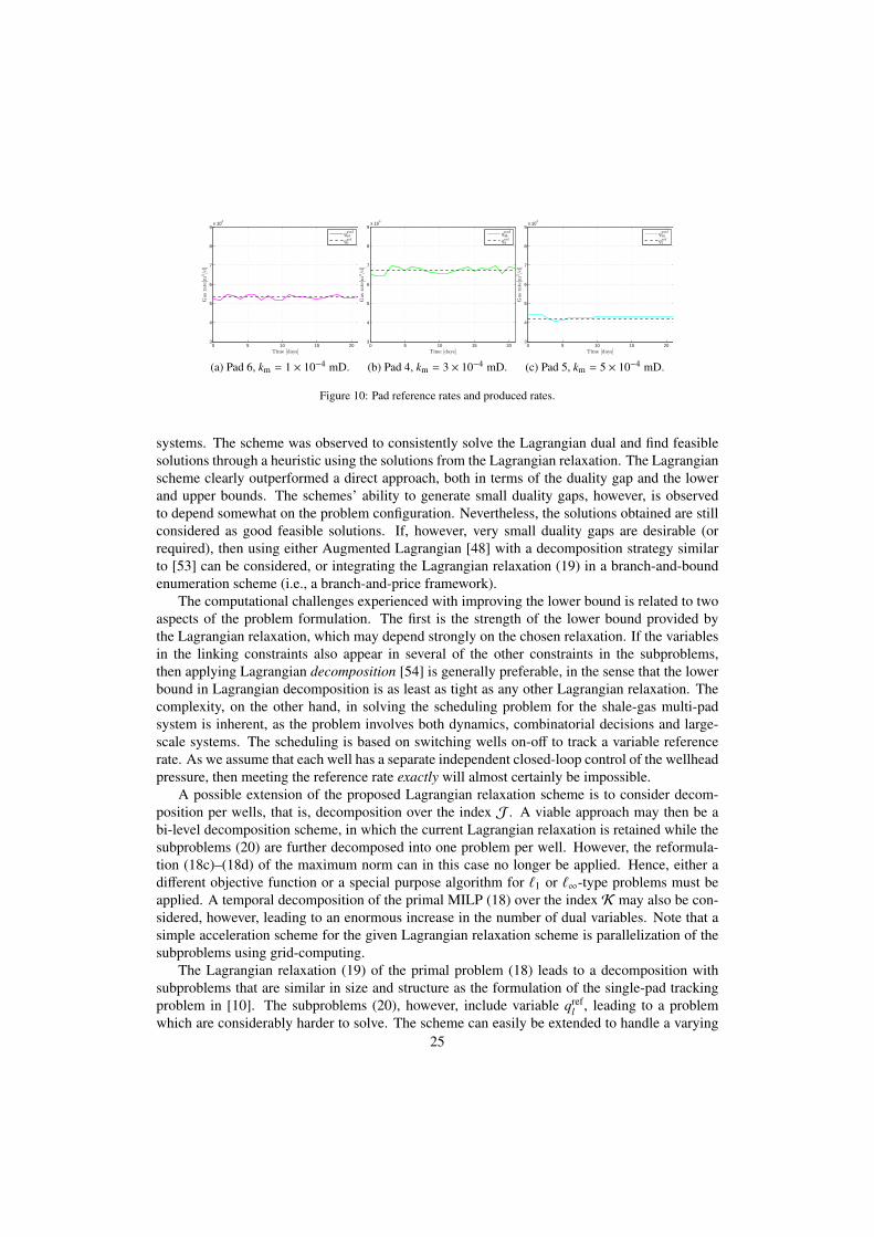
lk from the pads; the wells with the highestpermeability preserve a higher rate after shut-ins. Hence, fewer shut-ins are needed, and the totalrate from the pad is more stable as seen in Figure 10c.
0 5 10 15 204
4.5
5
5.5
6
6.5
x 105
Planning horizon [days]
Gas
rate
[m3/d]
Total produced rateqREF
Figure 9: Total rate from |L| = 9 pads with a three week planning horizon solved with the Lagrangian relaxation scheme.
7. Discussion
The main contribution in this paper is the development of a decomposable Lagrangian relax-ation scheme from a fullspace GDP formulation for field-wide shut-in scheduling in shale-gas
24
0 5 10 15 203
4
5
6
7
8
9x 10
4
Time [days]
Gas
rate
[m3/d]
qpad6k
qref6
(a) Pad 6, km = 1 × 10⁻⁴ mD.
0 5 10 15 203
4
5
6
7
8
9x 10
4
Time [days]
Gas
rate
[m3/d]
qpad4k
qref4
(b) Pad 4, km = 3 × 10⁻⁴ mD.
0 5 10 15 203
4
5
6
7
8
9x 10
4
Time [days]
Gas
rate
[m3/d]
qpad5k
qref5
(c) Pad 5, km = 5 × 10⁻⁴ mD.
Figure 10: Pad reference rates and produced rates.
systems. The scheme was observed to consistently solve the Lagrangian dual and find feasiblesolutions through a heuristic using the solutions from the Lagrangian relaxation. The Lagrangianscheme clearly outperformed a direct approach, both in terms of the duality gap and the lowerand upper bounds. The schemes’ ability to generate small duality gaps, however, is observedto depend somewhat on the problem configuration. Nevertheless, the solutions obtained are stillconsidered as good feasible solutions. If, however, very small duality gaps are desirable (orrequired), then using either Augmented Lagrangian [48] with a decomposition strategy similarto [53] can be considered, or integrating the Lagrangian relaxation (19) in a branch-and-boundenumeration scheme (i.e., a branch-and-price framework).
The computational challenges experienced with improving the lower bound is related to twoaspects of the problem formulation. The first is the strength of the lower bound provided bythe Lagrangian relaxation, which may depend strongly on the chosen relaxation. If the variablesin the linking constraints also appear in several of the other constraints in the subproblems,then applying Lagrangian decomposition [54] is generally preferable, in the sense that the lowerbound in Lagrangian decomposition is as least as tight as any other Lagrangian relaxation. Thecomplexity, on the other hand, in solving the scheduling problem for the shale-gas multi-padsystem is inherent, as the problem involves both dynamics, combinatorial decisions and large-scale systems. The scheduling is based on switching wells on-off to track a variable referencerate. As we assume that each well has a separate independent closed-loop control of the wellheadpressure, then meeting the reference rate exactly will almost certainly be impossible.
A possible extension of the proposed Lagrangian relaxation scheme is to consider decom-position per wells, that is, decomposition over the index J . A viable approach may then be abi-level decomposition scheme, in which the current Lagrangian relaxation is retained while thesubproblems (20) are further decomposed into one problem per well. However, the reformula-tion (18c)–(18d) of the maximum norm can in this case no longer be applied. Hence, either adifferent objective function or a special purpose algorithm for `1 or `∞-type problems must beapplied. A temporal decomposition of the primal MILP (18) over the index K may also be con-sidered, however, leading to an enormous increase in the number of dual variables. Note that asimple acceleration scheme for the given Lagrangian relaxation scheme is parallelization of thesubproblems using grid-computing.
The Lagrangian relaxation (19) of the primal problem (18) leads to a decomposition withsubproblems that are similar in size and structure as the formulation of the single-pad trackingproblem in [10]. The subproblems (20), however, include variable qref
l , leading to a problemwhich are considerably harder to solve. The scheme can easily be extended to handle a varying
25
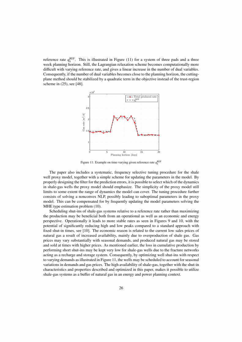
reference rate qREFk . This is illustrated in Figure (11) for a system of three pads and a three
week planning horizon. Still, the Lagrangian relaxation scheme becomes computationally moredifficult with varying reference rate, and gives a linear increase in the number of dual variables.Consequently, if the number of dual variables becomes close to the planning horizon, the cutting-plane method should be stabilized by a quadratic term in the objective instead of the trust-regionscheme in (25), see [48].
0 5 10 15 20
1
1.5
2
2.5
3
x 105
Planning horizon [days]
Gas
rate
[m3/d]
Total produced rateqREF
k
Figure 11: Example on time-varying given reference rate qREFk
The paper also includes a systematic, frequency selective tuning procedure for the shalewell proxy model, together with a simple scheme for updating the parameters in the model. Byproperly designing the filter for the prediction errors, it is possible to select which of the dynamicsin shale-gas wells the proxy model should emphasize. The simplicity of the proxy model stilllimits to some extent the range of dynamics the model can cover. The tuning procedure furtherconsists of solving a nonconvex NLP, possibly leading to suboptimal parameters in the proxymodel. This can be compensated for by frequently updating the model parameters solving theMHE type estimation problem (10).
Scheduling shut-ins of shale-gas systems relative to a reference rate rather than maximizingthe production may be beneficial both from an operational as well as an economic and energyperspective. Operationally it leads to more stable rates as seen in Figures 9 and 10, with thepotential of significantly reducing high and low peaks compared to a standard approach withfixed shut-in times, see [10]. The economic reason is related to the current low sales prices ofnatural gas a result of increased availability, mainly due to overproduction of shale gas. Gasprices may vary substantially with seasonal demands, and produced natural gas may be storedand sold at times with higher prices. As mentioned earlier, the loss in cumulative production byperforming short shut-ins may be kept very low for shale-gas wells due to the fracture networksacting as a recharge and storage system. Consequently, by optimizing well shut-ins with respectto varying demands as illustrated in Figure 11, the wells may be scheduled to account for seasonalvariations in demands and gas prices. The high availability of shale-gas, together with the shut-incharacteristics and properties described and optimized in this paper, makes it possible to utilizeshale-gas systems as a buffer of natural gas in an energy and power planning context.
26

8. Conclusions
In this work, a novel Lagrangian relaxation based scheme for shut-in scheduling in shale-gas multi-pad systems has been presented. The shut-in scheduling is integrated in field-wideproduction planning based on demands in gas-rate, and it is shown how production objectivesand constraints at different levels in the large-scale system can be included in the formulation.The decomposable scheme is scalable in the number of pads and shown through computationaltesting to outperform a direct approach for all sizable problems, though the efficiency of thescheme is observed to decrease for long planning horizons.
9. Acknowledgments
This work was supported by the Center for Integrated Operations in the Petroleum Industry,Trondheim, Norway (IO center). The authors gratefully acknowledge valuable feedback fromProfessor Curtis H. Whitson at NTNU, and financial support from an IBM PhD scholarship.
References
[1] Annual Energy Outlook 2011, Tech. Rep., The U.S. Energy Information Administration, 2011.[2] Z. Dong, S. A. Holditch, D. A. Mcvay, W. B. Ayers, Global Unconventional Gas Resource Assessment, SPE
Economics & Management 4 (4) (2012) 222–234.[3] R. Stefik, K. Paulson, When Unconventional Becomes Conventional, Journal of Canadian Petroleum Technology
50 (11) (2011) 68–70.[4] C. D. Jenkins, C. M Boyer II, Coalbed- and Shale-Gas Reservoirs, Journal of Petroleum Technology 60 (2) (2008)
92–99.[5] J. Baihly, R. Altman, R. Malpani, F. Luo, Shale Gas Production Decline Trend Comparison Over Time and Basins,
in: SPE Annual Technical Conference and Exhibition, Florence, Italy, sPE 135555, 2010.[6] C. H. Whitson, S. D. Rahmawati, A. Juell, Cyclic Shut-in Eliminates Liquid-Loading in Gas Wells, in: SPE/EAGE
European Unconventional Resources Conference and Exhibition, March, Vienna, Austria, SPE 153073, 2012.[7] H. Al Ahmadi, A. Almarzooq, R. Wattenbarger, Application of Linear Flow Analysis to Shale Gas Wells - Field
Cases, in: SPE Unconventional Gas Conference, Pittsburgh, Pennsylvania, USA, SPE 130370-MS, 2010.[8] J. F. Lea, H. V. Nickens, Solving Gas-Well Liquid-Loading Problems, Journal of Petroleum Technology 56 (4)
(2004) 30–36, SPE 72092.[9] N. Dousi, C. Veeken, P. K. Currie, Numerical and Analytical Modeling of the Gas-Well Liquid-Loading Process,
SPE Production & Operations 21 (4) (2006) 6–9.[10] B. R. Knudsen, B. Foss, Shut-in Based Production Optimization of Shale-gas Systems, Computers and Chemical
Engineering doi:10.1016/j.compchemeng.2013.05.022.[11] B. Knudsen, B. Foss, C. Whitson, A. Conn, Target-rate Tracking for Shale-gas Multi-well Pads by Scheduled Shut-
ins, in: IFAC Proceedings of the International Symposium on Advanced Control of Chemical Processes, Singapore,107–113, 2012.
[12] B. Foss, V. Gunnerud, M. Duenas Dıez, Lagrangian Decomposition of Oil-Production Optimization Applied to theTroll West Oil Rim, SPE Journal 14 (4).
[13] C. Sagastizabal, Divide to conquer: decomposition methods for energy optimization, Mathematical Programming134 (1) (2012) 187–222.
[14] J. Warren, P. Root, The Behavior of Naturally Fractured Reservoirs, SPE Journal 3 (3) (1963) 245–255.[15] M. Karimi-Farad, L. J. Durlofsky, K. Aziz, An Efficient Discrete-Fracture Model Applicable for General-Purpose
Reservoir Simulators, SPE Journal 9 (2) (2004) 227–236.[16] C. L. Cipolla, E. Lolon, J. Erdle, B. Rubin, Reservoir Modeling in Shale-Gas Reservoirs, SPE Reservoir Evaluation
& Engineering 13 (4) (2010) 638–653.[17] R. P. Sutton, S. A. Cox, R. D. Barree, Shale Gas Plays : A Performance Perspective, in: SPE Tight Gas Completions
Conference, San Antonio, Texas, USA, sPE 138447-MS, 2010.[18] R. O. Bello, R. A. Wattenbarger, Modelling and Analysis of Shale Gas Production With a Skin Effect, Journal of
Canadian Petroleum Technology 49 (12) (2010) 37–48.
27
[19] R. Al-Hussainy, H. R. Jr., P. Crawford, The Flow of Real Gases Through Porous Media, Journal of PetroleumTechnology 18 (5) (1966) 624–636.
[20] C. H. Whitson, M. R. Brule, Phase Behavior, vol. 20 of SPE Monograph Series, Society of Petroleum Engineers,2000.
[21] R. Turner, M. Hubbard, A. Dukler, Analysis and Prediction of Minimum Flow Rate for the Continuous Removalof Liquids from Gas Wells, Journal of Petroleum Technology 21 (11) (1969) 1475–1482.
[22] S. B. Coleman, H. B. Clay, D. G. Mccurdy, H. L. Norris III, A New Look at Predicting Gas-Well Load-Up, Journalof Petroleum Technology 43 (3) (1991) 329–333.
[23] R. Jayakumar, V. Sahai, A. Boulis, A Better Understanding of Finite Element Simulation for Shale Gas Reservoirsthrough a Series of Different Case Histories, in: SPE Middle East Unconventional Gas Conference and Exhibition,Muscat, Oman, SPE 142464, 2011.
[24] L. Ljung, System Identification: Theory for the user, Prentice Hall, second edn., 1999.[25] W. Spinelli, L. Piroddi, M. Lovera, On the role of prefiltering in nonlinear system identification, IEEE Transactions
on Automatic Control 50 (10) (2005) 1597–1602.[26] M. L. Thompson, M. A. Kramer, Modeling chemical processes using prior knowledge and neural networks, AIChE
Journal 40 (8) (1994) 1328–1340.[27] T. A. Johansen, Identification of non-linear systems using empirical data and prior knowledgean optimization
approach, Automatica 32 (3) (1996) 337–356.[28] SENSOR Manual, Coats Engineering Inc., 2009.[29] D. L. Katz, R. L. Lee, Natural Gas Engineering, McGraw-Hill Publishing Company, 1990.[30] A. Brooke, D.Kendrick, A. Meeraus, R. Raman, GAMS - A user’s guide, 2011.[31] B. Foss, J. P. Jensen, Performance Analysis for Closed-Loop Reservoir Management, SPE Journal 16 (1) (2011)
183–190, doi:10.2118/138891-PA.[32] H. P. Bieker, O. Slupphaug, T. A. Johansen, Real-Time Production Optimization of Oil and Gas Production Systems
: A Technology Survey, SPE Production & Operations 22 (4) (2007) 382–391.[33] C. V. Rao, J. B. Rawlings, J. H. Lee, Constrained linear state estimation - a moving horizon approach, Automatica
37 (10) (2001) 1619–1628.[34] R. Raman, I. E. Grossmann, Modelling and computational techniques for logic based integer programming, Com-
puters & Chemical Engineering 18 (7) (1994) 563–578.[35] I. E. Grossmann, F. Trespalacios, Systematic Modeling of Discrete-Continuous Optimization Models through Gen-
eralized Disjunctive Programming, AIChE Journal doi:10.1002/aic.[36] G. L. Nemhauser, L. A. Wolsey, Integer and Combinatorial Optimization, John Wiley & Sons, Inc., 1988.[37] A. Vecchietti, I. E. Grossmann, Modeling issues and implementation of language for disjunctive programming,
Computers & Chemical Engineering 24 (2000) 2143–2155.[38] E. Balas, Disjunctive programming and a hierarchy of relaxations for discret optimization problems., SIAM Journal
on Algebraic and Discrete Methods 6 (3) (1985) 466–486.[39] A. Vecchietti, S. Lee, I. E. Grossmann, Modeling of discrete/continuous optimization problems: characterization
and formulation of disjunctions and their relaxations, Computers & Chemical Engineering 27 (3) (2003) 433–448.[40] R. Raman, I. Grossmann, Relation between MILP modelling and logical inference for chemical process synthesis,
Computers & Chemical Engineering 15 (2) (1991) 73–84.[41] S. Takriti, B. Krasenbrink, L. S.-Y. Wu, Incorporating fuel constraints and electricity spot prices into the stochastic
unit commitment problem, Operations Research 48 (2) (2000) 268–280.[42] Y. Pochet, L. A. Wolsey, Production Planning by Mixed Integer Programming, Springer, 2006.[43] J. Lee, J. Leung, F. Margot, Min-up/min-down polytopes, Discrete Optimization 1 (1) (2004) 77–85.[44] D. Rajan, S. Takriti, Minimum Up / Down Polytopes of the Unit Commitment Problem with Start-Up Costs, Tech.
Rep., IBM Research Report, 2005.[45] A. M. Geoffrion, Lagrangian Relaxation and its Uses in Integer Programming, Mathematical Programming Study
2 (1974) 82–114.[46] A. Frangioni, About Lagrangian Methods in Integer Optimization, Annals of Operations Research 139 (1) (2005)
163–193.[47] J. E. Kelley, The Cutting-Plane Method for Solving Convex Programs, Journal of the Society for Industrial and
Applied Mathematics 8 (4) (1960) 703–712.[48] J.-B. Hiriart-Urruty, C. Lemarechal, Convex Analysis and Minimization Algorithms: part II, Springer, 1993.[49] S. Mouret, I. E. Grossmann, P. Pestiaux, A new Lagrangian decomposition approach applied to the integration of
refinery planning and crude-oil scheduling, Computers & Chemical Engineering 35 (12) (2011) 2750–2766.[50] B. Kallehauge, J. Larsen, O. B. Madsen, Lagrangian duality applied to the vehicle routing problem with time
windows, Computers & Operations Research 33 (5) (2006) 1464–1487.[51] R. E. Marsten, W. W. Hogan, J. W. Blankenship, The Boxstep Method for Large-Scale Optimization, Operations
Research 23 (2) (1975) 389–405.
28
[52] M. Fischetti, A. Lodi, Local branching, Mathematical Programming 98 (1-3) (2003) 23–47.[53] Z. Li, M. G. Ierapetritou, Capacity Expansion Planning Through Augmented Lagrangian Optimization and Sce-
nario Decomposition, AiChE Journal 58 (3).[54] M. Guignard, S. Kim, Lagrangean Decomposition: A Model Yielding Stronger Lagrangian Bounds, Mathematical
Programming 39 (2) (1987) 215–228.[55] R. K. Martin, Large Scale Linear and Integer Optimization: A Unified Approach, Kluwer Academic Publishers,
1998.
Appendix A. Proof of bound on dual variable
For proving the bound on λ ≥ −1, we can consider the following simplified Lagrangianrelaxation subproblem (20):
min f + λqref (A.1a)s.t.
f ≥ qref − qpad, (A.1b)
f ≥ −qref + qpad, (A.1c)
qPad ≤ U, (A.1d)
f , qref, qPad ≥ 0, (A.1e)
where we for simplicity have omitted the indices k and l. The variables f , qref are block sep-arable from the remaining variables defining the feasible set of (20), while the total rate qPad
is defined by a polytope Q2 spanned by (18e)–(18w) for given l ∈ L, i.e. a bounded polyhe-dron [36]. Consequently we can deduce an upper bound U on qPad. Consider the general LP,ZLP = min{cT x : Ax ≥ b, x ≥ 0}, and the corresponding symmetric dual LP, ZLPDual = max{bT u :AT u ≤ c, u ≥ 0}. By weak duality, the primal LP is feasible if and only if its corresponding dualLP is feasible. Similarly, the primal LP is unbounded if the dual LP is infeasible [36]. Hence,by considering the feasible set AT u ≤ c, u ≥ 0 for the dual LP of (A.1) parametrized by λ, weobtain the linear inequalities,
u1 + u2 ≤ 1, (A.2a)−u1 + u2 ≤ λ, (A.2b)
u1 − u2 − u3 ≤ 0, (A.2c)−u1 ≤ 0, (A.2d)−u2 ≤ 0, (A.2e)−u3 ≤ 0. (A.2f)
Feasibility requirements of the above inequalities can be derived by Fourier-Motzkin elimination,see e.g. [55]. By successively eliminating u1 and u2 by pairing the inequalities (A.2), we obtain
29
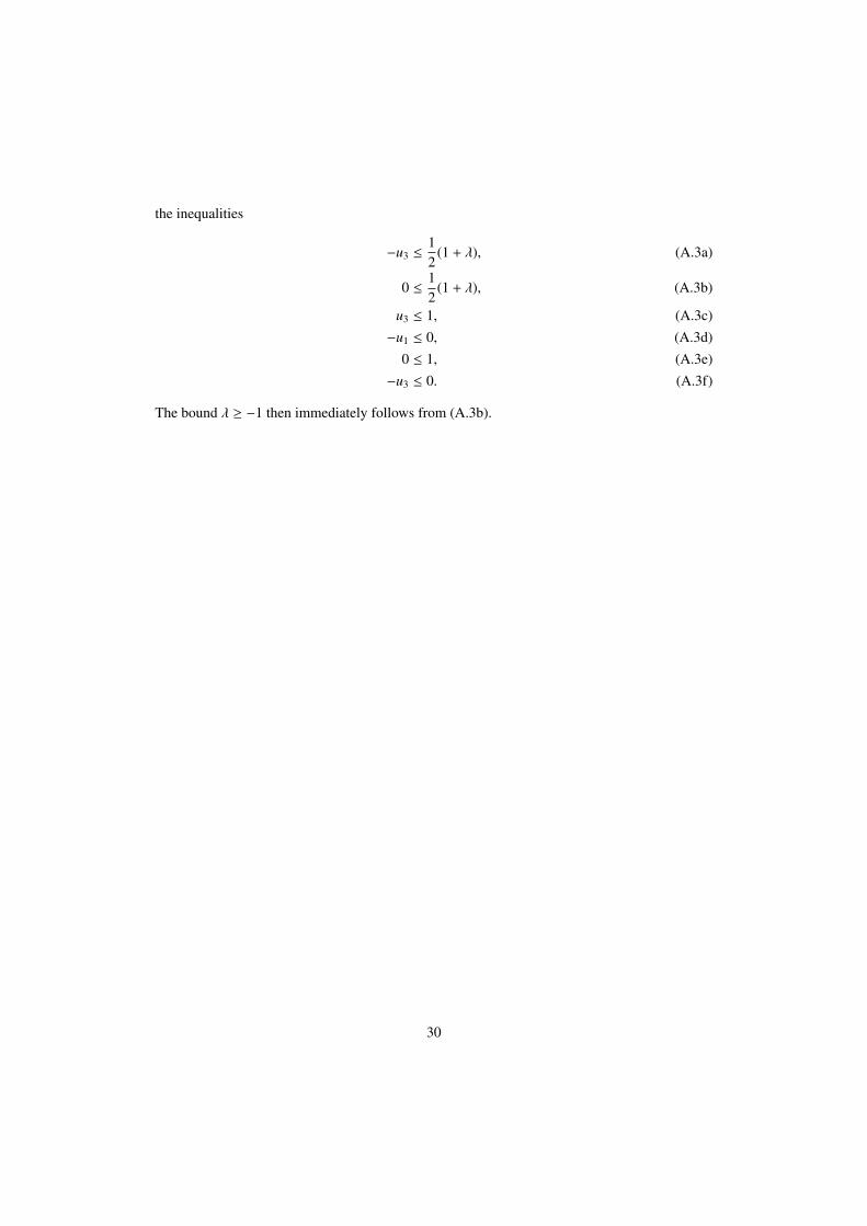
the inequalities
−u3 ≤12
(1 + λ), (A.3a)
0 ≤12
(1 + λ), (A.3b)
u3 ≤ 1, (A.3c)−u1 ≤ 0, (A.3d)
0 ≤ 1, (A.3e)−u3 ≤ 0. (A.3f)
The bound λ ≥ −1 then immediately follows from (A.3b).
30