land fragmentation and its implications for productivity ... working paper 2005/01 land...

ASARC Working Paper 2005/01

Land Fragmentation and its Implications for Productivity: Evidence from Southern India

Raghbendra Jha, Hari K. Nagarajan, Subbarayan Prasanna ASARC, RSPAS NCAER, New Delhi Indian Institute of ANU, Canberra Management, Bangalore

All correspondence to: Prof. Raghbendra Jha, Australia South Asia Research Centre, RSPAS, Division of Economics, Australian National University, Canberra, ACT 0200, Australia Fax: + 61 2 6125 0443 Email: [email protected]

mailto:[email protected]

Land Fragmentation and its Implications for Productivity

I. Introduction

In developing economies land reform, in particular land redistribution has occupied a central

role in debates about poverty — particularly chronic poverty — alleviation in rural areas.

Even if it were accepted that land redistribution could alleviate poverty the enthusiasm for

such redistribution needs to be tempered with consideration of the potential efficiency effects

of land fragmentation. The fragmentation of land holdings could rise with land fragmentation.

In turn, land fragmentation could lead to sub-optimal usage of factor inputs and thus to lower

overall returns to land. The factors contributing to this could be losses due to extra travel

time, wasted space along borders, inadequate monitoring, and the inability to use certain

types of machinery such as harvesters.

Fragmentation of land is widespread in India and it is believed that fragmented nature

of land holdings may play a major role in explaining low levels of agricultural productivity.

Despite substantial rise in yields India ranks 34th in yields for sugarcane, 57th for cotton, 118th

for pulses, and, 51st for rice although India is a leading producer of each of these crops in

aggregate terms.1 Further, there is evidence of inefficient use of resources in agriculture and

the resulting increases in costs, e.g., 25 times more water/tonne of output is being used to

irrigate Cotton in India than in Egypt.

In response to the perceived adverse effects of land fragmentation the then Finance

Minister allocated Rs. 5 million over a period of five years, as an incentive for land

consolidation, in his 2000 budget speech. However, the Planning Commission of India has

indicated a near complete failure on this front.

To date, however, there has been no systematic attempt at quantifying the effects of

land fragmentation and understanding the channels through which these effects operate. The

present paper attempts to fill this void.

In this paper, we undertake a detailed assessment of the consequences of land

fragmentation using a unique panel data set from Southern India, with comprehensive

information on all landholding households in two contiguous villages over a five-year

period. In particular, we examine whether technical efficiency of farm production is

significantly related to farm size, whether yield is importantly impacted by the degree of

fragmentation as measured by the number of plots, average plot size, and an index of

1 Economic Survey 1998–99.

ASARC Working Paper 2005/01 1

fragmentation,2 and whether such fragmentation impacts upon labor allocations. We then use

stochastic production function methods to measure the degree of technical efficiency and

relate this to the degree of land fragmentation. Our results show clearly that land

fragmentation has a significant adverse effect on land productivity.

The plan of this paper is a follows. In section II we review the literature on this issue

whereas section III discusses the data asset. Section IV details the methodology and

estimation procedure, section V presents the results and section VI concludes.

II. A Brief Literature Review

An important consideration in an evaluation of the consequences of land fragmentation for

technical yields is whether economic processes that reflect local agro-climatic conditions

drive such fragmentation. However, a more immediate reason for the overall patterns of land

fragmentation in rural Indian the prevalence of the Zamindari system in many of the river

valleys. The Zamindari system was characterized by highly inequitable pattern of land

holdings with very few landowners holding onto most of the cultivatable land. To correct this

inequitable pattern of land holding, the Indian Constitution (enacted in 1949), granted powers

to different states to enact land redistribution measures. These efforts were supplemented in

the early 1970s by the enactment of Land Ceiling Acts, which placed upper limits on land

holdings and required the surplus land to be redistributed among the landless. This process

along with the fragmentation through acts of succession from one generation to the next has

reduced size of land holdings and led to fragmentation of land holdings of farmers. As noted

earlier various laws designed to address the issue of fragmentation have met with only limited

success.3

2 The Januszewski index is defined as, ∑∑

=a

aK

where ‘a’ represents the parcel size. The index ranges between 0 and 1. 1 implies that the farmer holds all his land in the form of single plot. It has three properties: fragmentation increases (the value of the index decreases) as the number of plots increases, fragmentation increases when the range of plot sizes is small, and fragmentation decreases when the area of large plots increases and that of small plots decreases. Specifically, Januszewski’s index measures the number of plots and the size distribution of the plots.

3 The Bombay Prevention of Fragmentation and Consolidation Act 1947, provides for State intervention for consolidation of fragments irrespective of the willingness of the people. This act also provides various incentives for co-operation such as wavering of consolidation fee charged by the government and granting of Taccavi loans to agriculturists whose lands have been consolidated. The East Punjab Holdings Act 1948, empowered the Punjab Government to take up consolidation in any area either on the request of the holders of an area or, on its own initiative. The Bihar Consolidation of Holdings and Prevention of Fragmentation Act 1956, prohibits the creation of future fragments, a certain minimum area necessary for profitable cultivation to be defined as a standard minimum area and all holdings below that size to be treated as fragments.


The literature on land size and land productivity is large and has been around for

decades. In recent times Binswanger et. al. (1995) have argued that there is an inverse

relation between the tow whereas Banerjee and Ghatak (1996) have questioned this result.

Carlyle (1983), Heston and Kumar (1983), Bentley (1987), Blarel et al. (1992), Jabarin and

Epplin (1994)) have focused on the impact of fragmentation on yield and productivity. The

debate has focused basically on the impact of fragmentation on the ability of farmers to

minimize risk since fragmentation was perceived to have a negative impact on productivity

and yield.

The impact of land size on technical efficiency has been investigated in a series of

papers. The countries where this relationship has been studied include the Philippines (Herdt

and Mandac 1981; Kalirajan and Flinn 1983; Dawson and Linagard 1989), Brazil (Taylor and

Shonkwiler 1986), Tanzania (Shapiro 1983), Pakistan (Ali and Chaudhry 1989) and India

(Huang and Bagi 1984; Kalirajan 1981; Junankar 1980; Sidhu 1974; Lau and Yotopoulos

1971; Battese, Coelli and Colby 1989; Tadesse and Krishnamoorthy 1997; Kumbhakar and

Bhattacharya 1992; and, Jha and Rhodes 1999).4 These studies make use of stochastic

production function methods and conclude that the large variation in yield across farmers is

due to differences in technical efficiency, which is largely influenced by farm size, size of the

land holding, ecological factors and their interaction with factor inputs like land, technology

and fertilizer. However, to the best of our knowledge there does not exist any study linking

technical efficiency to land fragmentation. Part of the reason for this is the lack of reliable

data on land fragmentation. We address this issue by studying a unique primary data set

where information on such fragmentation and its evolution are collected.

III. The Data

The deltas at the ends of the river valley systems in India have traditionally been major

centers of agricultural production, with farmers adopting innovative methods of cultivation in

response to changing conditions and new technologies. In recent years, these regions have

been increasingly prone to water stress arising from either, a) depletion of ground water

resources through over-exploitation, and, b) river water disputes. The Kaveri Delta in Tamil

Nadu has been historically considered as a ‘rice bowl’ of southern India. This is the region in

which scientific methods of irrigation were developed as far back as the Chola period in the

8th century AD. One of these villages, in this region (Nelpathur) is also the place in which the 4 For a good review, see Sankar (1997) and Battese and Coelli (1992)


‘grow more food’ program — a precursor of the Green Revolution — in the late 1960s was

launched. This region is, however, currently seeing a general decline in rice production and

farmers are resorting to crop diversification.

The data for this study were collected over a 5-year period beginning 1995 in 2

contiguous villages (Nelpathur and Thirunagari) situated in the Sirkhazi taluk of the

Thanjavur district of Tamil Nadu, India. These villages are located in the Kaveri Delta.

Thirunagari is a larger village as compared to Nelpathur. According to the 1991 Census the

number of households in Nelpathur is 550 whereas it is 881 in Thirunagari. The population in

Nelpathur is 2237 whereas in Thirunagari it is 3700. The number of children below the age of

6 is 306 in Nelpathur whereas in Thirunagari it is 410. Around 19% of the Thirunagari village

population is engaged in farming (165 households). Nelpathur has a greater proportion (28%)

of the population engaged in agricultural activities. There are 1250 acres of cultivable land in

Nelpathur and 2000 acres in Thirunagari. The number of agricultural workers is 1500 in

Thirunagari and 1200 in Nelpathur. There is no noticeable forest cover in any of these

villages. In Thirunagari, government canals irrigate 1100 acres of cultivable land while such

canals in Nelpathur irrigate 700 acres.

Figure 1 here

The survey data were collected for 137 farmers of the Nelpathur village and 83 farmers of

Thirunagari, for the period 1995–1999. Farmers were asked questions regarding their land

holdings, crops grown, output produced, inputs used and ownership of factors of production.

Data was also collected on the price paid by the farmers for the factor inputs used and the

price they receive for their output (both from the traders and the government). Information

was obtained for the number of plots owned by the farmers, the size of each of these plots

and the crops grown in these plots. Questions regarding the outputs of different crops grown

by the farmers and the revenue obtained from these crops were also a part of the

questionnaire. Farm input data is in terms of the quantity and the total cost spent on seeds,

fertilizers, irrigation, bullocks, cartage, manure and machinery, general labor, labor for land

preparation, and labor for harvesting and threshing. Tables 1 to 2 and Figures 2 to 7 describe

the data.

Tables 1 to 2 and Figures 2 to 7 here


IV. Methodology

The basis for our empirical investigations is the estimation of a generalized translog cost

function (Christensen and Green 1976) of the form:

( )

∑∑∑∑ +++

Χ+++=

iititYi

i jjtitij

iiti

ititYYitYit

PYPPP

YYC

lnlnlnln21ln

ln)(ln21lnln 2

0

γγα

θγαα (1)

where γij = γji, Cit is total cost of production of i-th farmer in t-th year, Yit is output, and the

Pit’s are the prices of the factor inputs and, Xit is the variable with respect to which scale

economies have to be tested. Xit can be farm-size, number of plots cultivated or the average

plot-size (only one Xit variable is used at any one time). In order to correspond to a well-

behaved production function, a cost function must be homogeneous of degree one in prices,

i.e., for a fixed level of output; the total cost must increase in proportion to the increases in

prices. This implies the following relationship among the parameters,

∑ ∑∑∑∑∑ =====

i iijijijYi

ii 0 ,0 ,1

jii

γγγγα

In the presence of constant returns to scale, θ =1. Scale economies are indicated by a

coefficient of less than one and scale diseconomies by a coefficient that is grater than one.

Analogously the effects of fragmentation and landsize on yields may be estimated using a

translog production function,

∑∑∑ ++=i j

jtitiji

itiit xxxy lnln21lnln 0 ββα (2)

where βij = βji , and xit’s are per acre input factors and yit is the output per acre.

Production function estimation may also be used to test for possible heterogeneity in

the productivity of labor input. In particular, consider

( )iti j

jtitiji

itiit pXXXY lnlnln21lnln 0 θββα +++= ∑∑∑ (3)

where βij = βji , and Y is the logarithm of the outputs of Samba, Black Gram and Cotton, Xi’s

are the inputs namely various kinds of labor inputs, acreage, fertilizer, pesticide, bullocks,

machinery and irrigation (number of hours), and, pit is defined below, depending on the

nature of heterogeneity being tested:

a) For intra-activity labor heterogeneity:


pit = hired labor/(hired labor + family labor)

tivity A + Hired

In case of intra-activity labor heterogeneity, a negative and significant θ indicates that hired

b) For inter-activity labor heterogeneity :

pit = hired labor in activity A/(hired labor in ac

labor in activity B).

labor is inefficient as compared to family-provided labor. A positive and significant but

below unity value suggests that hired labor is more efficient, but the difference in marginal

productivity of these two types of labor declines as hired labor increases in importance in the

labor force. A positive but greater than unity value of θ indicates that hired labor is more

efficient and the difference in marginal productivity of these two types of labor increases as

hired labor increases in importance in the labor force. An insignificant value of θ suggests

that there is no difference between the marginal productivity of the two kinds of labor. To

address whether supervision decreases labor heterogeneity one may also condition production

on levels of supervision in different activities.

( ) bitaititi j

jtitiji

itiit SSpXXXY +++++= ∑∑∑ lnlnln21 ββα lnln 0 θ (4)

where, Sait and Sbit represent the supervision hours devoted to activity A and B respectively.

.

Consid

Examination of technical efficiency is carried out using a translog functional form

er the stochastic frontier production function5 for panel data,

itititit UVtXfY −+= ),,( β (5)

where Yit is the output (or the loga of the output) of the i-th farmer in the t-th timrithm e

period; Xit is a (k×1) vector of (transformations of the) input quantities of the i-th farmer in

the t-th time period; f(.) is a suitable functional form of the production function, β is a (1×k)

vector of unknown parameters to be estimated; t is a time trend representing technical

change; Vi’s are random errors which are assumed to i.i.d. N(0, 2vσ ), and independent of the

Ui’s; the Ui’s are non-negative random variables assumed account for technical

inefficiency in production and are assumed to be independently distributed, such that U

to

i is

obtained by truncation (at zero) of the normal distribution with mean, δiz , and variance, 2uσ ;

5 See Battese, Coelli and Rao (1999).


zi is a (m×1) vector of explanatory variables associated with technical inefficiency of

production of farmers over time; and δ is an (1×m) vector of unknown coefficients.

Equation (5) specifies the stochastic frontier production function in terms of the

original production values. However, the technical inefficiency effects, the Ui’s are assumed

to be a function of a set of explanatory variables, the zi’s, and an unknown vector of

coefficients, δ. The explanatory variables in the inefficiency model may include some input

variables in the stochastic frontier, provided the inefficiency effects are stochastic. If the first

z-variable has value one and the coefficients of all other z-variables are zero, then this case

represents the model specified in Stevenson (1980) and Battese and Coelli (1988, 1992). If all

elements of the δ-vector are equal to zero, then the technical inefficiency effects are not

related to the z-variables and so the half-normal distribution originally specified in Aigner,

Lovell and Schmidt (1977) is obtained. If interactions between farm-specific variables and

input variables are included as z-variables, then a non-neutral stochastic frontier, proposed in

Huang and Liu (1994), is obtained.

The technical inefficiency effect, Ui, in the stochastic frontier model (5) could be

specified in equation (6),

iii WzU += δ (6)

where the random variable, Wi, is defined by the truncation of the normal distribution with

zero mean and variance, σ such that the point of truncation is 2u , δiz− , i,e., Wi ≥ δiz− . e

assumptions are consistent with U

Thes

i being a non-negative truncation of the N( δiz , )-

distribution.

2uσ

Huang and Liu (1994) proposed an interesting generalization of the above

specification. They permitted interaction effects between the variables in the stochastic

production frontier, Xi, and the determinants of inefficiency, zi. Thus the frontier itself is

subjected to non-neutral shifts. In this case the Ui in equation (6) are modified to read:

iiiii WXzzU ++= ** δδ (7)

where is a vector of values of appropriate interaction terms between the variables in

z

ii Xz *

i and Xi and δ* is a vector of unknown parameters to be estimated.

The method of maximum likelihood is proposed for simultaneous estimation of the

parameters of the stochastic frontier and the model for the technical inefficiency effects. The


likelihood function and its partial derivatives with respect to the parameters of the model are

presented in Battese and Coelli (1993). The likelihood function is expressed in terms of the

variance parameters, and . 222uvs σσσ +≡ su

22 / σσγ ≡

The technical efficiency of production for the i-th firm is defined by (7),

( ) ( iiii WzUTE )−−=−= δexpexp (7)

The prediction of the technical efficiencies is based on its conditional expectation, given the

model assumptions.

The reduced form representation of the translog production function is as follows,

ititttt

j kiktijtjk

jijttit

UVtt

XXXY

−+++

++= ∑∑∑2

0 lnln21ln)ln(

ββ

βββ (8)

where the technical inefficiency effects are assumed to be defined by

ittttj

ijtjzoit WttzU ++++= ∑ 2)( δδδδ (9)

where the subscript i and t represent the i-th farmer and the t-th year of operation, Yit is (the

logarithm of) the Tornqvist index of the outputs of Samba and Blackgram or Samba and

Cotton;6 β’s and δ’s are the unknown parameters to be estimated; t = 1,… 5 is a time trend for

the duration of the panel. Vit and Wit are as defined in the previous section; Xit are the

independent variables, the inputs; zijt are the variables that are supposed to determine the

inefficiency. Table 7 lists the Xi variables and zi variables used in the estimation.

Table 7 here We use both male-female wage gap and wage gap between farm labor and non-farm labor as

determinants of inefficiency. The wage gap (between farm labor and non-farm labor) is

6 If Y represents the outputs of crop k in period t produced by farmer i, and Wikt ikt the value share for output of

crop k in period t, then the Tornqvist index in its log-change form is given by,

( iktikti

iktiktst YY

WWY lnln

2ln −⎟

⎠⎞

⎜⎝⎛ +

= ∑ ) where s and t represent the time periods.


defined as the difference between the wage paid to the hired agricultural worker and the wage

received by the same agricultural worker during off-farm season in brick-kilns and prawn

farms. This gap appeared around 1994–95 and has led to a rise in agricultural wages. In

addition to this the viability of the second crop after Rice (especially Samba rice) is

dependent on the availability of hired labor. The second crop usually is grown when the

brick-kilns and the prawn farms are in operation. Hence the labor supply during the period

when the second crop is grown is seriously truncated. This has consequences in the form of

less than the optimal quantity of labor being available to the farmers growing the second

crop. Therefore we believe that the wage gap will impact the technical efficiency of

cultivation of the crop sequences.

The inefficiency frontier model (8)-(9) accounts for both technical change and time-

varying inefficiency effects. The time variable in the stochastic frontier (8) accounts for

Hicksian neutral technological change. However, the time variable in the inefficiency model

(9) species that the inefficiency effects may change linearly with respect to time. The

distributional assumptions on the inefficiency effects permit the effects of technical change

and time-varying behavior of the inefficiency effects to be identified, in addition to the

intercept parameters, βo, and δo, in the stochastic frontier and the inefficiency model. Time

outside the frontier is used as a factor that could create non-neutrality. This is in line with the

logic that with the passage of time, the technology in use could influence the rate of

substitution between factors of production. The fixed effects from the estimation of equation

(4) for the different crops are used as determinants of inefficiency. These fixed effects

explain the impact of fragmentation on technical efficiency.

V. Estimation Procedure

The general model of the stochastic frontier (4) along with the technical inefficiency effects

(5) can be simultaneously estimated by maximum likelihood method with the null hypothesis

for no technical inefficiency effects 0:0 =γH . The parameter γ lies between 0 and 1 and

this range can be searched to provide a good starting value for use in the iterative

maximization process such as Davidson-Fletcher-Powell (DFP) algorithm. We use the

FRONTIER 4.1 of Coelli (1996) to estimate the models. If the null hypothesis is accepted

this would mean that σu2 is zero and therefore would mean that the Ui’s should be removed

from the model, leaving a specification with parameters that can be consistently estimated

using ordinary least squares.


VI. Results

We turn to discussing the results of the estimation procedure used to examine the relationship

between fragmentation and technical efficiency. We proceed to discuss the results

progressively.

i. There is a significant positive relationship between farm size, average plot size and

yield. This test is conducted for two dominant crop sequences in these villages namely

Samba-Blackgram and Samba-Cotton. However there is a negative relationship between

number of plots cultivated and the yields of these crop-sequences. More importantly, the

magnitude of this relationship differs as one goes from Samba-Blackgram to Samba-

Cotton.

Table 3a here

From these results one can infer that fragmentation (as measured by number of plots)

has a negative impact on yields and consequently is a problem to be addressed.

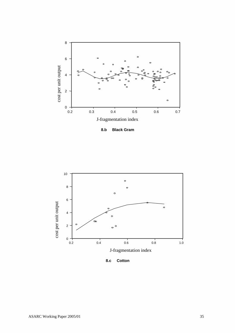
ii. The test for no economies of scale with respect to number of plots cultivated is strongly

rejected in the case of both Samba-Blackgram and Samba-Cotton. This then implies that

it will be optimal for the farmers to have the land holdings in fewer plots. In fact it is

interesting and revealing to note that complete fragmentation might not be a desired

outcome for all the farmers in these villages. This is evident by the shape of the SRAC

curve with respect to fragmentation. This then suggests that consolidation should result

in farmers holding “optimal number of plots”.

Figure 8 here

However there are significant economies of scale with respect to both farm-size and

plot-size. This result is interesting in the context of current distribution of land holdings

in these villages that suggests a preponderance of small and marginal landholders.

Hence farmers should be provided incentives to consolidate their land holdings.

Farmers should also look into the possibility of increasing farm-size through leasing-in,

purchases, co-operative farming etc.


Table 3b here

iii. There is strong evidence to suggest that the family-provided labor is less efficient than

the hired labor for different crops and for different activities for each crop.

Table 4 here

These results suggest that farmers can achieve the desired level of efficiency by hiring

labor for different activities. The results also indicate that for Samba-Blackgram the

current level of input-mix (hired and family-provided) is about close to optimal

(indicated by low values of the coefficient). However for Samba-Cotton the hired labor

intensities could be increased.

iv. Given the preceding result there will be tendency on the part of the farmers to hire

inputs. Hired inputs need not be homogeneous in terms of their respective efficiency.

Input heterogeneity (especially labor heterogeneity) can lead to significant reduction in

technical efficiency. Hence it is important for us to determine the magnitude of such

heterogeneity. The results indeed show that there are significant levels of heterogeneity

in performance of hired labor across different activities for different crops.

Table 5 here

It is believed that most of this labor heterogeneity is caused by land fragmentation.

However this is a proposition that needs to be tested. Impact of land fragmentation

needs to be empirically tested. Impact of land fragmentation on efficiency of specific

factors of production is as such a phenomenon yet to be established. Farmers, who have

hired factor inputs, engage in a level of supervision to ensure efficiency of these inputs.

We are able to show that hired supervision is able to reduce labor heterogeneity

significantly. These results are shown in tables. We posit here that any residual labor

heterogeneity is caused by land fragmentation.


a) The impact of fragmentation on labor heterogeneity is estimated after controlling for

fixed effects for fragmentation on output. We are able to establish a clear causation

between fragmentation and fixed effects for different crop sequences. We find that a

significant number of these fixed effects are caused by fragmented landholdings.

When equation (4) was estimated controlling for fragmentation we find both

positive and negative fixed effects. This causality suggests that there could be

returns to fragmentation for such farmers (reinforced by our finding on the shape of

the average short run cost curve). Irrespective of the sign of the fixed effects we find

a significant causality between fragmentation and fixed effects which suggests that

the impact of fragmentation on technical efficiency is likely to be indirect rather

than direct.

Figures 9 here

In order to fully capture the impact of these fixed effects on technical efficiency we

choose to use these as factors determining inefficiency.

vi. The estimates of the stochastic frontier are shown in Tables 6. The variables used for

estimation are described in Table 7.

Tables 6, and, 7 here

The joint frontier is accepted in favor of independent frontier. We note that following

significant results from the estimation process -

a) Farm size has a positive impact on technical efficiency.

b) The male-female wage-gap is a significant phenomenon in these villages. Such a

wage-gap contributes significantly to technical inefficiency. However we note that

this gap matters only for the crop sequence Samba-Cotton.

c) In both these villages localized non-farm employment is on the rise. Brick-kiln and

prawn-farms are popular sources of non-farm employment during specific seasons

that overlaps the cultivation of second crop (Blackgram or Cotton). The wage-gap

between farm and non-farm activity significantly tends to reduce technical

efficiency.


d) We test the impact of fragmentation on technical efficiency by using the fixed

effects caused by fragmentation on different activities. These fixed effects on an

average tend to produce significant negative impacts on technical efficiency. Hence

we are not able to completely reject the hypothesis that fragmentation has a negative

impact on technical efficiency. This is an added evidence to suggest that farmers on

an average want to posses their holdings in optimal number of plots.

VII. Conclusions

This paper has shown that fragmentation has a significant impact on technical efficiency. The

policies must be designed to allow for consolidation to take place. However one should

understand that even if markets are allowed to function. Potential consolidation may not take

place and farmers may choose to hold a specific number of plots. We in fact see such a

phenomenon when the average variable cost is examined in relation to fragmentation.

The impact of fragmentation as measured by fixed effects illustrates the fact that

fragmentation has both negative and positive effects on technical efficiency. In fact we

indeed find some of the positive effects of such fixed effects quite significantly large. Hence

if consolidation has to occur through markets than a level of fragmentation is inevitable.


References

Afriat, S.N. (1972), “Efficiency Estimation of production Functions”, International Economic Review,13: 568–98.

Aigner, D.J., Lovell, C.A.K. and Schmidt, P. (1977). “Formulation and Estimation of Stochastic Frontier Production Functions”, Journal of Econometrics, 6: 21–37.

Battese,G.E., T.J. Coelli and T.C. Colby (1989), “Estimation of Frontier Production Functions and the Efficiencies of Indian farms Using Panel Data from ICRISAT’s Village Level Studies”, Journal of Quantitative Economics, 5: 327–48.

Battese, G.E., and T.J. Coelli (1992), “Frontier Production Functions, Technical Efficiency and Panel Data: With Application to Paddy farmers in India”, Journal of Productivity Analysis, 3, pp. 153–69.

Battese, G.E., and T.J. Coelli (1993), “A Stochastic Frontier production Function Incorporating a Model for Technical Inefficiency Effects”, Working Papers in Econometrics and Applied Statistics, No. 69, Department of Econometrics, University of New England, Armidale.

Battese, G.E., and T.J. Coelli (1995), “A Model for Technical Inefficiency Effects in a Stochastic Frontier Production Function for Panel Data”, Empirical Economics, 20: 325–32.

Bardhan, P.K. (1973), “Size, Productivity and Returns to Scale: An analysis of farm level data in Indian agriculture”, Journal of Political Economy, 81: 1370–86.

Battese, G.E., G.S. Corra (1977), “Estimation of a production frontier model with application to the pastoral zone of Eastern Australia”, Australian.Journal of Agricultural Economics, 21: 169–79.

Banerjee, Abhijit and Maitreesh Ghatak (1996), “Empowerment and Efficiency: The Economics of Tenancy Reform”, Mimeo MIT and University of Chicago.

Binswanger, Hans, Klaus Deininger and Gershan Feder (1995), “Power, Distortions, Revolt and Reform in Agricultural Land Relations”, in Behrman, Jere and T.N. Srinivasan, eds, Handbook of Development Economics (Amsterdam: Elsevier).

Blarel, Benoit, et al. (1992), “The Economics of Farm Fragmentation: Evidence from Ghana and Rwanda”, World Bank Economic Review, 6(2): pp. 233–54.

Carlyle, W.J. (1983), “Fragmentation and Consolidation in Manitoba”, Can. Geogr., 27: 17–34.

Cornwell, C., P. Schmidt, and R.C. Sickles (1990), “Production Frontiers with Cross-sectional and Time-series Variation in Efficiency Levels”, Journal of Econometrics, 46: 185–200.

Coelli, T.J. (1995a), “Estimators and Hypothesis Tests for a Stochastic Frontier Function: A Monte Carlo Analysis”, Journal of Productivity Analysis, 6: 247–68.

Coelli, T.J. (1995b), “Measurement and Sources of Technical Inefficiency in Australian Electricity Generation”, paper presented at the New England Conference on Efficiency and Productivity, University of New England, Armidale, November 23–24.


Coelli, T.J. (1996a), “A Guide to FRONTIER Version 4.1: A Computer Program for Frontier Production Function Estimation”, CEPA Working Paper 96/07, Department of Econometrics, University of New England, Armidale.

Cornwell, C., P. Schmidt and R.C. Sickles (1990), “Production Frontiers with Cross-sectional and Time-series Variation in Efficiency Levels”, Journal of Econometrics, 46: 185–200.

Dawson, P.J., Lingard, J. (1989), “Measuring Farm Efficiency Over Time on Philippine Rice Farms”, Journal of Agricultural Economics, 40: 168–77.

Farrell, M.J. (1957), “The Measurement of Productive Efficiency”, Journal of the Royal Statistical Society, Series A, CXX, Part 3: 253–90.

Greene, W.H. (1980a), “Maximum Likelihood Estimation of Econometric Frontier Functions”, Journal of Econometrics, 13: 27–56.

Herdt, R.W. and A.M. Mandac (1981), “Modern Technology and Economic Efficiency of Philippine Rice Farmers”, Economic Development and Cultural Change, 29(2): 375–99.

Heston, Alan; Dharma Kumar (1983), “The persistence of land fragmentation in peasant agriculture: An analysis of South Asian Cases”, Explorations in Economic History, 20: 199–220

Huang, C.J., F.S. Bagi (1984), “Technical efficiency on Individual Farms in Northwest India”, Southern Economist Journal, 51: 108–15.

Huang, C.J. and J.T. Liu (1994), “Estimation of Non-Neutral Stochastic Frontier Production Function”, Journal of Productivity Analysis, 5(2): 171–80.

Jabarin, S. A.and F.M Epplin (1994, “Impacts of Land Fragmentation on the Cost of Producing Wheat in the Rain-fed Region of Northern Jordan”, Agricultural Economics, 11: 191–6.

Jha, R.; M.J. Rhodes (1998), “Technical Efficiency, Farm Productivity and Farm Size in Indian Agriculture”.

Jha ,R and M.J. Rhodes (1999), “Some imperatives of the Green Revolution: technical efficiency and ownership of inputs in Indian agriculture”, Agriculture and Resource Economics Review.

Junankar, P.N. (1980), “Test of the Profit Maximization Hypothesis: A Study of Indian agriculture”, Journal of Development Studies.16: 187–203.

Kalirajan, K.P. (1981), “An Econometric Analysis of Yield Variability in Paddy Production”, Canadian Journal of Agricultural Economics, 29: 283–94.

Kalirajan, K.P. and J.C. Flinn (1983), “The Measurement of Farm Specific Technical Efficiency”, Pakistan Journal of Applied Economics, 2(1): 167–80.

Kumbhakar, S.C. (1990), “Production Frontiers, Panel Data and Time-varying Technical Inefficiency”, Journal of Econometrics, 46: 201–11.

Kumbhakar, S.C. and A. Bhattacharyya (1992), “Price Distortions and Resource-use Inefficiency in Indian Agriculture: A restricted profit function approach, Review of Economic Statistics, 74: 231–9.


Kumbhakar, S. and L. Hjalmarsson (1993), “Technical Efficiency and Technical Progress in Swedish Dairy Farms”, in H. Fried, K. Lovell and S. Schmidt, eds, The Measurement of Productive Efficiency: Techniques and Applications, New York, Oxford University Press.

Lau, L.J., P.A. Yotopoulos (1971), “A test for relative efficiency and application to Indian agriculture”. American Economic Review, 61: 94–109.

Meeusen, W., J. Van den Broeck (1977), “Efficiency Estimation from Cobb-Douglas Production Functions with Composed Error”, International Economic Review, 34: 163–73.

M. Ahmad and Boris E. Bravo-Ureta (1996), “Technical Efficiency Measures for Dairy farms using panel data: A comparison of Alternative Model specifications”, The Journal of Productivity Analysis, 7: 399–415.

M. Ali and M.A. Chaudhry (1989), “Inter-Regional Farm Efficiency in Pakistan’s Punjab: A Frontier production function study”.

Peter Schmidt and Robin Sickles (1990), “Production Frontiers with cross-sectional and Time-Series Variation in Efficiency Levels”, Journal of Econometrics, 46: 185–200. Reprinted in The Econometrics of Panel Data, vol. 2, Maddala, ed., Cheltenham: Edward Elger,(1993).

Piesse J and C. Thirtle (2000), “A Stochastic Frontier Approach to Firm Level Efficiency, Technological Change and Productivity during the Early Transition in Hungary”, Journal of Comparative Economics. 28, 473–501

Pitt, M.M., and L-F. Lee (1981), “Measurement and Sources of Technical Inefficiency in the Indonesian Weaving Industry”, Journal of Development Economics, 9: 43–64.

Richmond, J. (1974), “Estimating the Efficiency of Production”, International Economic Review, 15: 515–21.

Schmidt, P. and R.C. Sickles (1984), “Production Frontiers and Panel Data”, Journal of Business and Economic Statistics, 2: 367–74.

Seale, J.L., Jr. (1990), “Estimated Stochastic Frontier Systems with Unbalanced Panel Data: The case of floor title manufacturers in Egypt”, Journal of Applied Econometrics, 5: 59–74.

Shapiro, K.H. (1983), “Efficiency Differentials in Peasant Agriculture and their Implications for Development Policies”, Journal of Development Studies, 19(2): 179–90.

Sidhu, S.S. (1974), “Relative Efficiency in Wheat Production in the Indian Punjab”, American Economic Review, 64: 742–51.

Tadesse, B. and S. Krishnamoorthy (1997), “Technical Efficiency in Paddy Farms of Tamil Nadu: An Analysis based on farm size and ecological zone”, Agricultural Economics, 16 (3), 185–92.

Taylor, G.T. and J.S. Shonkwiler (1986), “Alternative Stochastic Specifications of the Frontier Production Function in the Analysis of Agricultural Credit Programs and Technical Efficiency”, Journal of Development Economics, 21: 149–60.


Table 1 : Village wise summary of crops grown and main inputs used

Average Std.Dev. Minimum Maximum Number of farmers

Nelpathur

Samba Acreage (acre) 3.15 5.44 0.28 48.04 137 Output (Kg) 5740.62 9910.15 276 85800 137 Yield (Kg/acre) 1359.50 387.37 360.87 2819.55 137 Black Gram Acreage (acre) 2.96 5.37 0.28 48.29 124 Output (Kg) 906.64 1547.37 80 13308 124 Yield (Kg/acre) 261.46 67.76 72 451.12 124 Cotton Acreage (acre) 2.64 1.55 0.66 6.60 18 Output (Kg) 2695.11 1269.44 800 6000 18 Yield (Kg/acre) 1184.8 190.8 900 1875 18 Total inputs used Cartage (no. of trips) 11 16 2 125 113 Hired labor (no. of labor days) 307 449 26 3906 137 Family provided Labor (no. of labor days) 65 27 2 123 86 Seed purchases (Kg) 164 346 2 1575 30 Seed family provided (Kg) 179 276 16 2149 128 Pesticide (Ltr) 272 1187 8 13241 135

Thirunagari

Samba Acreage (acre) 1.54 1.01 0.32 6.13 83 Output (Kg) 2982.29 1792.68 900 10800 83 Yield (Kg/acre) 1656.1 255.25 1194.69 2531.25 83 Black Gram Acreage (acre) 1.52 0.95 0.32 6.13 80 Output (Kg) 496.31 275.42 180 1800 80 Yield (Kg/acre) 294.5 51.81 206.9 506.25 80 Cotton Acreage (acre) 2.21 1.60 0.79 3.95 3 Output (Kg) 2733.33 1921.80 1000 4800 3 Yield (Kg/acre) 1248 28.5 1215.19 1265.8 3 Total inputs used Cartage (no. of trips) 6 4 2 24 79 Hired labor (no. of labor days) 164 110 46 655 83 Family provided Labor (no. of labor days) 70 15 4 98 61 Seed purchases (Kg) 30 47 3 100 4 Seed family provided (Kg) 81 48 29 300 82 Pesticide (Ltr) 68 70 14 462 83


Table 2 : Profit margin and coefficient of variation*

Small farmers Medium farmers Large farmers

Year Avg profit CV Avg profit CV Avg profit CV

Samba

1995 0.1 23.61 -0.02 0.13 9.37 1996 0.3 9.36 0.19 14.47 -0.09 1997 0.68 4.76 0.24 16.81 0.69 1.5 1998 0.86 3.38 0.72 4.05 0.94 0.73 1999 1.03 2.75 0.46 10.03 1.39 0.55

Black Gram

1995 6.85 0.09 6.83 0.1 6.16 0.23 1996 6.92 0.1 6.94 0.11 6.07 0.21 1997 11.92 0.06 11.86 0.07 11.33 0.16 1998 8.02 0.09 8.14 0.1 7.45 0.22 1999 11.58 0.07 11.68 0.09 11.25 0.16

Cotton

1995 9.76 0.07 9.87 0.06 10.22 0.04 1996 11.26 0.08 11.38 0.07 11.76 0.04 1997 11.94 0.07 11.9 0.09 12.49 0.04 1998 13.9 0.1 13.67 0.08 14.67 0.09 1999 15.16 0.09 14.92 0.07 15.8 0.09

Samba-Black Gram

1995 6.93 0.38 6.71 0.46 6.42 0.31 1996 7.21 0.42 7.06 0.44 6.01 0.36 1997 12.6 0.27 11.85 0.41 12.14 0.18 1998 8.96 0.35 8.8 0.37 8.41 0.24 1999 12.75 0.23 11.86 0.45 12.62 0.17

Samba-Cotton

1995 9.06 0.24 10.34 0.13 10.03 0.07 1996 10.97 0.22 12.1 0.13 12.03 0.07 1997 11.68 0.25 12.89 0.15 13.3 0.06 1998 13.22 0.21 15.32 0.14 15.15 0.06 1999 15.18 0.22 16.51 0.14 16.62 0.04

* Small farmers : Farmers with less than 2 acres. Medium farmers : Farmers with 2 to 4 acres. Large farmers : Farmers with 4 or greater than 4 acres


Table 3:

3.a: Yield as a function of farm size, Number of plots cultivated and Average plot size

Farm size Number of plots cultivated Average plot size Samba-Blackgram 0.0344 -0.0244 0.0301 (0.002) (0.01) (0.001) Samba-cotton 0.2509 -0.2407 0.1518 (0.006) (0.000) (0.000)

3.b: Testing for Economies of scale w.r.t. Farm size, Number of plots and Average plot size

Farm size Number of plots cultivated Average plot size Samba-Blackgram 0.050 1.844 0.119 (0.000) (0.000) (0.000)

Samba-cotton 0.049 2.912 0.047 (0.000) (0.002) (0.001)

Table 4: Test of heterogeneity between hired and family labor7

Samba

Hired Land preparation 0.2843

(0.029)

Sowing 0.0257 (0.560)

Transplanting 0.2598 (0.002)

Fertilizer and Pesticide Application 0.3369 (0.238)

Harvesting 0.3316 (0.000)

Black Gram

Sowing 0.0701

(0.008) Harvesting 0.0304

(0.837)

Cotton

Land preparation (earthing) 0.6983 (0.165)

Sowing 0.6583 (0.010)

Harvesting (picking) 0.0265 (0.932)

7 No family labor was employed for weeding operations.


Table 5 : Test of heterogeneity between hired labor employed for various activities*

5.1.a Samba: Pre supervision efficiency gap land preparation Sowing transplanting irrigation weeding fertilizer/pesticide application harvesting

Land preparation 0

Sowing 0.1568 0 (0.103)

Transplanting 0.0678 1.112 0 (0.193)

(0.089)

Irrigation -0.1969 0.7831 -0.5746 0 (0.028)

(0.084) (0.012)

Weeding 0.2149 0.1172 0.9325 0.1247 0 (0.037)

(0.097) (0.001) (0.004)

Fertilizer/pesticide application 0.4616 0.1769 0.3796 0.5569 0.2129 0 (0.129)

(0.061) (0.054) (0.000) (0.069)Harvesting -0.3272 1.6813 -0.4063 0.7504 0.8335 1.2678 0

(0.000) (0.000) (0.000) (0.000) (0.000) (0.000)

5.1.b Samba: Post supervision efficiency gap

land preparation Sowing transplanting irrigation weeding fertilizer/pesticide application harvestingLand preparation 0

Sowing 0.1449 0

(0.131)

Transplanting 0.054 0.954 0

(0.302)

(0.137)Irrigation -0.0154 0.313 -0.1023 0

(0.073)

(0.011) (0.110)Weeding 0.1934 0.1139 0.7561 -0.0104 0

(0.063)

(0.101) (0.008) (0.835)Fertilizer/pesticide application 0.4301 0.1683 0.2033 0.3744 0.1943 0

(0.157)

(0.067) (0.308) (0.020) (0.100)Harvesting -0.319 1.5191 -0.3897 0.3721 0.8009 1.0636 0

(0.000) (0.000) (0.000) (0.000) (0.000) (0.000)

* The activities in the rows are in the numerator and the activities in the columns form the denominator.

5.2.a Black Gram: Pre supervision efficiency gap

sowing Harvesting

Sowing 0

Harvesting 0.02639 0 (0.073)

5.2.b Black Gram: Post supervision efficiency gap

sowing Harvesting

Sowing 0

Harvesting 0.02637 0 (0.074)

5.3.a Cotton: Pre supervision efficiency gap

Earthing sowing irrigation weeding fertilizer/pesticide application picking

earthing 0

sowing 2.0902 0 (0.087)

irrigation 0.4089 0.5677 0 (0.264) (0.105)

weeding -0.4904 0.6454 -0.6599 0 (0.260) (0.007) (0.000)

fertilizer/pesticide application 0.3661 0.9317 -0.5044 -0.5617 0 (0.138) (0.005) (0.092) (0.049)

picking 0.4102 0.8102 0.6135 0.3587 0.3109 0 (0.388) (0.080) (0.003) (0.020) (0.124)

5.3.b Cotton: Post supervision efficiency gap

Earthing sowing irrigation weeding fertilizer/pesticide application picking

earthing 0

sowing 1.1144 0 (0.465)

irrigation 0.3418 0.4006 0 (0.406) (0.283)

weeding -0.1912 -0.1227 -0.178 0 (0.648) (0.675) (0.352)

fertilizer/pesticide application 0.0533 -0.1577 -0.2539 -0.1432 0 (0.890) (0.684) (0.416) (0.644)

picking 0.177 -0.435 0.1851 -0.0918 -0.0289 0 (0.721) (0.629) (0.414) (0.623) (0.898)


Table 6.a : Stochastic Frontier Results for both villages :Samba-Blackgram

Coefficient t-ratio Variable beta 0 10.561 24.546 intercept beta 1 3.363 15.258 ln(acreage) beta 2 0.040 0.227 ln(harvesting-threshing labor) beta 3 -0.602 -4.097 ln(threshing-machine) beta 4 -0.138 -1.328 ln(general labor) beta 5 0.244 2.831 ln(nursery labor) beta 6 0.013 2.402 ln(bull) beta 7 -2.127 -16.348 ln(seeds) beta 8 -0.009 -0.190 ln(irrigation-hrs) beta 9 -0.019 -0.810 ln(potash) beta10 0.298 10.701 ln(acreage)^2 beta11 0.105 6.306 ln(land-preparation-labor)^2 beta12 0.004 0.940 ln(pesticide)^2 beta13 0.040 4.374 ln(cartage)^2 beta14 0.015 1.111 ln(general-labor)^2 beta15 0.020 0.953 ln(nursery-labor)^2 beta16 0.017 2.856 ln(seeds)^2 beta17 -0.007 -0.876 ln(irrigation-hrs)^2 beta18 0.007 0.888 ln(DAP)^2 beta19 -0.003 -0.686 ln(urea)^2 beta20 0.016 3.102 ln(potash)^2 beta21 0.051 10.030 time beta22 -0.075 -1.733 ln(acreage)*ln(supervision-labor) beta23 -0.162 -5.599 ln(land-preparation-labor)*ln(supervision-labor) beta24 -0.238 -4.579 ln(harvesting-threshing-labor)*ln(supervision-labor) beta25 -0.058 -2.619 ln(pesticide)*ln(supervision-labor) beta26 0.121 2.573 ln(threshing-machinery)*ln(supervision-labor) beta27 -0.052 -2.239 ln(supervision-labor)*ln(nursery-labor) beta28 0.345 12.640 ln(supervision-labor)*ln(seeds) beta29 0.002 0.286 ln(supervision-labor)*ln(irrigation-hrs) beta30 -0.675 -15.167 ln(acreage)*ln(seeds) beta31 0.246 8.279 ln(harvesting-threshing-labor)*ln(seeds) beta32 0.049 2.564 ln(pesticide)*ln(seeds) beta33 0.019 0.759 ln(threshing-machinery)*ln(seeds) beta34 0.018 1.674 ln(seeds)*ln(DAP) beta35 -0.014 -2.433 ln(seeds)*ln(potash) sigma-squared 0.375 6.686 gamma 0.964 145.436 delta 1 1.194 5.538 Time delta 2 -0.107 -5.714 Time^2 delta 3 0.957 6.075 Village dummy delta 4 0.610 5.893 Wage gap (brick kiln) delta 5 0.215 7.446 Owned no. of plots delta 6 -6.026 -4.705 Weeding vs. land preparation (fixed effects) delta 7 -11.423 -5.022 Transplanting vs. sowing labor (fixed effects) delta 8 7.327 7.033 Irrigation vs. sowing labor (fixed effects) delta 9 -38.529 -8.316 Sowing vs. weeding labor (fixed effects) delta10 -2.765 -2.209 Sowing vs. pesticide labor (fixed effects) delta11 37.058 6.913 Sowing vs. harvesting labor (fixed effects) delta12 9.675 7.154 Transplanting vs. weeding labor (fixed effects) delta13 -10.824 -7.749 Transplanting vs. pesticide labor (fixed effects) delta14 11.319 6.239 Transplanting vs. harvesting labor (fixed effects) delta15 10.441 5.444 Pesticide vs. harvesting labor (fixed effects) delta16 -0.051 -3.347 Acreage

log of the likelihood function: 353.087 LR test of the one-sided error: 206.722


Table 6.b: Stochastic Frontier Results for both villages: Samba-Cotton

Coefficient t-ratio variable

beta 0 -15.782 -13.325 ln(output) beta 1 1.433 8.167 ln(acreage) beta 2 5.708 6.390 ln(land-preparation labor) beta 3 -0.351 -4.841 ln(harvesting-threshing labor) beta 4 -0.651 -0.869 ln(pesticide) beta 5 0.194 1.446 ln(cartage) beta 6 16.371 24.879 ln(general labor) beta 7 -14.209 -19.849 ln(nursery labor) beta 8 -0.949 -6.462 ln(bull) beta 9 2.773 8.272 ln(seed) beta10 -1.312 -17.125 ln(irrigation-hrs) beta11 -3.683 -5.787 ln(DAP) beta12 -1.382 -3.867 ln(urea) beta13 -0.192 -5.390 ln(potash) beta14 0.662 11.089 ln(acreage)^2 beta15 -0.682 -6.631 ln(land-preparation labor)^2 beta16 -0.019 -0.239 ln(pesticide)^2 beta17 -0.123 -5.276 ln(machinery-day)^2 beta18 -0.190 -4.805 ln(cartage)^2 beta19 -1.698 -24.404 ln(general labor)^2 beta20 0.126 9.775 ln(supervision labor)^2 beta21 3.138 18.599 ln(nursery labor)^2 beta22 0.168 6.375 ln(bull)^2 beta23 -0.199 -6.784 ln(seed)^2 beta24 0.092 7.032 ln(irrigation-hrs)^2 beta25 0.360 5.125 ln(DAP)^2 beta26 0.116 3.499 ln(urea)^2 beta27 0.011 10.147 time^2 sigma-

squared 0.009 6.643

gamma 1.000 5031.547 delta 1 -0.075 -0.905 Time delta 2 0.021 1.759 time^2 delta 3 0.204 2.124 Dummy delta 4 0.072 1.870 Wage gap (male-female) delta 5 0.145 2.704 wage gap (brick-kiln) delta 6 0.029 3.717 total no. of plots cultivated delta 7 -0.710 -0.718 land preparation vs. transplanting labor (fixed effects) delta 8 -0.694 -0.727 land preparation vs. irrigation labor (fixed effects) delta 9 -1.014 -1.053 Weeding vs. land preparation labor (fixed effects) delta10 0.161 0.173 land preparation vs. pesticide labor (fixed effects) delta11 -0.817 -0.884 sowing vs. pesticide labor (fixed effects) delta12 1.137 1.238 Transplanting vs. harvesting labor (fixed effects) delta13 1.268 1.082 Irrigation vs. pesticide labor (fixed effects) delta14 0.228 0.187 Pesticide vs. harvesting labor (fixed effects) delta15 -0.006 -0.906 Acreage

log likelihood function: 133.720 LR test of the one-sided error: 21.685


Table 7: Description of variables used in frontier 7.1.a Samba-Blackgram :Inputs S. no Variable Description Unit of measurement 1 ln(acreage) Acreage commitment to the crop Acres 2 ln(harvesting-threshing labor) Labor for harvesting and threshing operations Labor-days 3 ln(threshing by machinery) Tractors used for threshing Days 4 ln(general labor) Labor used for weeding, irrigation and application of pesticides and fertilizers Labor-days 5 ln(nursery labor) Labor used in nursery for land preparation and seeding Labor-days 6 ln(bull) Bullocks used for land preparation and threshing Number of bullocks 7 ln(seeds) Quantity of seeds used Kilograms 8 ln(irrigation-hrs)

Irrigation of the crops

Hours

9

ln(potash) Fertilizer

Kilograms 10 ln(acreage)^2 11 ln(land-preparation-labor)^2

12 ln(pesticide)^2 13 ln(cartage)^2 14 ln(general-labor)^2 15 ln(nursery-labor)^2

16 ln(seeds)^2 17 ln(irrigation-hrs)^2

18 ln(DAP)^2 19 ln(urea)^2 20 ln(potash)^2 21 Time Year of production

22 Ln(acreage)*ln(supervision-labor) 23 Ln(land-preparation-labor)*ln (supervision-labor) 24 ln(harvesting-threshing-labor)*ln(supervision-labor)

25 ln(pesticide)*ln(supervision-labor) 26 ln(threshing-machinery)*ln(supervision-labor)

27 ln(supervision-labor)*ln(nursery-labor)

28 ln(supervision-labor)*ln(seeds) 29 ln(supervision-labor)*ln(irrigation-hrs)

30 ln(acreage)*ln(seeds) 31 ln(harvesting-threshing-labor)*ln(seeds)

32 ln(pesticide)*ln(seeds) 33 ln(threshing-machinery)*ln(seeds)

34 ln(seeds)*ln(DAP) 35 ln(seeds)*ln(potash)

7.1.b Samba-Blackgram: factors causing inefficiency S. no Variable Description Unit of measurement 1 Time Year of production 2

time^2 3 village dummy Dummy variable indicating membership to Nelpathur village 4 wage gap for brick kiln Wage gap between brick kiln workers and hired labor Rupees 5 owned no. of plots Total number of plots owned by the farmer 6 weeding -land preparation (fixed effects) Fixed effects from the comparison of land preparation labor vs weeding labor 7 transplanting -sowing labor (fixed effects) Fixed effects from the comparison of sowing labor vs transplanting labor 8 irrigation -sowing labor (fixed effects) Fixed effects from the comparison of sowing labor vs irrigation labor 9 sowing -weeding labor (fixed effects) Fixed effects from the comparison of sowing labor vs weeding labor 10 sowing-pesticide labor (fixed effects) Fixed effects from the comparison of sowing labor vs pesticide application labor 11 sowing -harvesting labor (fixed effects) Fixed effects from the comparison of sowing labor vs harvesting labor 12 transplanting -weeding labor (fixed effects) Fixed effects from the comparison of transplanting labor vs weeding labor 13 transplanting -pesticide labor (fixed effects) Fixed effects from the comparison of transplanting labor vs pesticide application labor 14 transplanting –harvesting labor (fixed effects) Fixed effects from the comparison of transplanting labor vs harvesting labor15 pesticide-harvesting labor (fixed effects) Fixed effects from the comparison of pesticide application labor vs harvesting labor16 Acreage Acreage commitment to the crop Acre

7.2.a Samba-Cotton :Inputs S. no Variable Description Unit of measurement 1 Acreage Acreage commitment to the crop Acres 2 Land-preparation labor Labor for leveling, seeding, transplanting nad land preparation Labor-days 3 Harvesting-threshing labor Labor for harvesting and threshing operations Labor-days 4 Pesticide Quantity of pesticides used Litres 5 Cartage Carts used for transporting output to threshing mills or to the market Number of cart trips 6 General labor Labor used for weeding, irrigation and application of pesticides and fertilizers Labor-days 7 Nursery labor Labor used in nursery for land preparation and seeding Labor-days 8 Bull Bullocks used for land preparation and threshing Number of bullocks 9 Seed Quantity of seeds used Kilograms 10 Irrigation-hrs

Irrigation of the crops Hours

11

DAP Fertilizer-Diammonium Phosphate

Litres12 Urea Fertilizer Kilograms 13 Potash Fertilizer

Kilograms

14 ln(acreage)^2 15 ln(land-preparation labor)^2

16 ln(pesticide)^2 17 ln(machinery-day)^2

18 ln(cartage)^2 19 ln(general labor)^2 20 ln(supervision labor)^2

21 ln(nursery labor)^2

22 ln(bull)^2 23 ln(seed)^2 24 ln(irrigation-hrs)^2

25 ln(DAP)^2 26 ln(urea)^2

27 time^2

7.2.b Samba-Cotton :factors causing inefficiency S. no Variable Description Unit of measurement 1 Time Year of production 2

time^2 3 Dummy Dummy variable indicating membership to Nelpathur village 4 wage male-female Wage gap between male and female labor Rupees 5 wage brick-kiln Wage gap between brick kiln workers and hired labor Rupees 6 total no. of plots Total number of plots being cultivated by a farmer 7 land preparation-transplanting labor (fixed effects) Fixed effects from the comparison of land preparation labor vs transplanting labor 8 land preparation-irrigation labor (fixed effects) Fixed effects from the comparison of land preparation labor vs irrigation labor9 weeding -land preparation labor (fixed effects) Fixed effects from the comparison of land preparation labor vs weeding labor 10 land preparation-pesticide labor (fixed effects) Fixed effects from the comparison of land preparation labor vs pesticide application labor 11 sowing -pesticide labor (fixed effects) Fixed effects from the comparison of sowing labor vs pesticide application labor 12 transplanting –harvesting labor (fixed effects) Fixed effects from the comparison of transplanting labor vs harvesting labor13 irrigation -pesticide labor (fixed effects) Fixed effects from the comparison of irrigation labor vs pesticide application labor14 pesticide -harvesting labor (fixed effects) Fixed effects from the comparison of pesticide application labor vs harvesting labor15 Acreage Acreage commitment to the crop Acre

Figure 1: Location of Nelpathur and Thirunagari villages

THIRUNAGARI

NELPATHUR


Figure 2 : Distribution of farm size in Nelpathur and Thirunagari

2.a Nelpathur

2.b Thirunagari


Figure 3 : Distribution of average plot size in Nelpathur and Thirunagari

3.a Nelpathur

3.b Thirunagari


Figure 4 : Pattern of holding of plots by farmers in Nelpathur and Thirunagari8

4.a Nelpathur

4.b Thirunagari

8 These figures do not include farmers owing a single plot


Figure 5 : Distribution of Rice Yield in Nelpathur and Thirunagari

5.a Nelpathur : Samba (Rabi Rice)

5.b Nelpathur: Kuruvai (Kharif Rice)

5.c Thirunagari :Samba (Rabi Ric

AS

ARC Working Paper 2005/01 33

Figure 6 : Distribution of Black Gram yield in Nelpathur & Thirunagari

6.a Nelpathur : Black Gram

6.b Thirunagari :Black Gram


Figure 7 : Distribution of Cotton yield in Nelpathur

7.a Nelpathur :Cotton

Figure 8: Relation between cost per unit output and fragmentation

2

4

6

8

10

12

00.2 0.4 0.6 0.8 1.0

cost

per

uni

t out

put

J-fragmentation index

8.a Samba

0

2

4

6

8

0.2 0.3 0.4 0.5 0.6 0.7

cost

per

uni

t out

put


8.b Black Gram

0

2

4

6

8

10

0.2 0.4 0.6 0.8 1.0

cost

per

uni

t out

put


8.c Cotton


Figure 9: Relationship between fixed effects and J-fragmentation index (Samba)

a) Tranplanting vs. Sowing Labor

.00

.04

.08

.12

.16

.20

.24

0.2 0.3 0.4 0.5 0.6 0.7 0.8 0.9 1.0

J-fragm enta tion index

Fixe

d ef

fect

s

b) Sowing vs. Weeding Labor

.00

.04

.08

.12

.16

.20

.24

0.2 0.3 0.4 0.5 0.6 0.7 0.8 0.9 1.0


Fixe

d ef

fect

s

i


c) Transplanting vs. Harvesting Labor

-.25

-.20

-.15

-.10

-.05

.000.2 0.3 0.4 0.5 0.6 0.7 0.8 0.9 1.0

J-fragm entation index

Fixe

d ef

fect

s

i

c) Weeding vs. Labor for Pesticide application

.00

.04

.08

.12

.16

.20

.24

0.2 0.3 0.4 0.5 0.6 0.7 0.8 0.9 1.0


Fixe

d ef

fect

s


land fragmentation and its implications for productivity ... working paper 2005/01 land...

Documents