land-ice elevation changes from photon-counting swath ... · instruments and methods land-ice...

Instruments and Methods

Land-ice elevation changes from photon-counting swath altimetry:first applications over the Antarctic ice sheet

Duncan A. YOUNG,1 Laura E. LINDZEY,1 Donald D. BLANKENSHIP,1

Jamin S. GREENBAUM,1 Alvaro GARCIA DE GORORDO,1 Scott D. KEMPF,1

Jason L. ROBERTS,2;3 Roland C. WARNER,2;3 Tas VAN OMMEN,2;3 Martin J. SIEGERT,4

Emmanuel LE MEUR5

1University of Texas Institute for Geophysics (UTIG), University of Texas at Austin, Austin, TX, USA2Australian Antarctic Division, Kingston, Tasmania

3Antarctic Climate and Ecosystems CRC, University of Tasmania, Hobart, Tasmania4University of Bristol, Bristol, UK

5Laboratoire de Glaciologie et Géophysique de l’Environnement, Grenoble, FranceCorrespondence: Duncan A. Young <[email protected]>

ABSTRACT. Satellite altimetric time series allow high-precision monitoring of ice-sheet mass balance.Understanding elevation changes in these regions is important because outlet glaciers along ice-sheetmargins are critical in controlling flow of inland ice. Here we discuss a new airborne altimetry datasetcollected as part of the ICECAP (International Collaborative Exploration of the Cryosphere by AirborneProfiling) project over East Antarctica. Using the ALAMO (Airborne Laser Altimeter with MappingOptics) system of a scanning photon-counting lidar combined with a laser altimeter, we extend the2003–09 surface elevation record of NASA’s ICESat satellite, by determining cross-track slope and thusindependently correcting for ICESat’s cross-track pointing errors. In areas of high slope, cross-trackerrors result in measured elevation change that combines surface slope and the actual �z=�t signal.Slope corrections are particularly important in coastal ice streams, which often exhibit both rapidlychanging elevations and high surface slopes. As a test case (assuming that surface slopes do not changesignificantly) we observe a lack of ice dynamic change at Cook Ice Shelf, while significant thinningoccurred at Totten and Denman Glaciers during 2003–09.

KEYWORDS: aerogeophysical measurements, Antarctic glaciology, glacier mapping, glaciologicalinstruments and methods, ice-sheet mass balance

INTRODUCTIONThe response of the Antarctic ice sheet to climate change is aprincipal unknown in determining potential sea-level rise(Church and others, 2013; IPCC, 2013). There is an emergingconsensus that the mass balance of the Antarctic ice sheet isnow negative (Vaughan and others, 2013), but uncertaintyremains in the magnitude and causes of this trend. Onlyprolonged time series of relevant observations can resolvethese uncertainties (Wouters and others, 2013), and onlydetailed observations of ice thickness, surface elevation andbasal boundary conditions, tied to better-constrained modelsof ice physics, will allow predictions of future mass change tobe made. In particular, the East Antarctic ice sheet (EAIS)contribution to sea-level rise is poorly constrained (Vaughanand others, 2013), due to sparse ice-thickness measurementsand limited coverage of surface-elevation change data alongits remote 8000 km long margin.Altimetry of the ice-sheet surface provides a powerful

constraint on ice-sheet mass balance and behavior. Inco-herent orbital radar altimeters (e.g. Envisat (Flament andothers, 2014)), which are not interrupted by cloud cover,yield long time series and have the capacity to provide greatcoverage of coastal Antarctica; however, they have limitedhorizontal resolution (a few kilometers) and strong sensitivity

to surface slopes. Coherent orbital radar altimetry, currentlyrepresented by CryoSat-2 (McMillan and others, 2014;Siegfried and others, 2014), can improve footprint resolutionto less than 0:5 km� 1:5 km. However, issues of variablesurface penetration remain. In contrast, orbital and airbornelaser altimeters offer smaller footprint sizes restricted to thesurface interface. The single-beam Geoscience Laser Altim-eter System (GLAS), on board the Ice, Cloud and landElevation Satellite (ICESat; Schutz and others, 2005) operatedbetween 2003 and 2009, with footprints �80m wideseparated by 175m. ICESat repeated a pattern of orbitaltracks up to 15 times over its 6 year lifetime, to retrieve high-resolution records of surface elevation change. However,ICESat suffered pointing errors of up to hundreds of meters inthe cross-track direction, and these errors complicate theinterpretation of repeat-track elevation change where signifi-cant cross-track slopes are present.A follow-on mission for ICESat, ICESat-2, will address the

cross-track problem using multiple pairs of fixed beamsspaced by 90m on the ground; in order to deploy thesemultiple beams, a new low-power lidar technology, photoncounting (Degnan, 2002), will be deployed on ICESat-2’sAdvanced Topographic Laser Altimeter System (ATLAS). Tocontinue the time series between ICESat and the expected

Journal of Glaciology, Vol. 61, No. 225, 2015 doi: 10.3189/2015JoG14J048 17

https://www.cambridge.org/core/terms. https://doi.org/10.3189/2015JoG14J048Downloaded from https://www.cambridge.org/core. IP address: 54.191.40.80, on 20 Aug 2017 at 02:43:44, subject to the Cambridge Core terms of use, available at

https://www.cambridge.org/core/terms

https://doi.org/10.3189/2015JoG14J048

https://www.cambridge.org/core

2017 launch of ICESat-2, NASA initiated the OperationIceBridge airborne program to conduct repeated altimetryobservations of key regions. As part of this program, theInternational Collaborative Exploration of the Cryosphere byAirborne Profiling (ICECAP) consortium collected a 3 yearsurface-elevation dataset acquired over East Antarctica usingan advanced airborne scanning photon-counting lidar (PCL),coupled to a legacy nadir-pointing laser profiler (here calledthe LAS).ICECAP systematically targeted high-leverage ICESat

tracks for re-flight to extend the surface-elevation record, inparticular for tracks where clouds had interrupted the ICESatrecord. We use the well-characterized LAS system to provideprofile measurements of surface elevation, in tandem withthe PCL (which has higher absolute range uncertainties)which provides cross-track slope information for correctionof ICESat observations. Together the LAS and PCL form theAirborne Laser Altimeter with Mapping Optics (ALAMO).We first describe the context for surface-elevation change

in this region, including the existing ICESat record. We thendescribe the LAS and PCL components of the altimetrysystem and its operation, using the example of the 2011ICECAP field season (ICP4). We discuss our approach for thegeneration of data products to address the OperationIceBridge science goals. We then extend our coverage toall three years of field campaigns, and focus on three keysites along the Indo-Pacific margin of East Antarctica.

THE 2003–09 ICESat OBSERVATION RECORDAfter its launch in 2003, ICESat conducted seventeen 33 daycampaigns of altimetry observations, which have led tonumerous discoveries about the mass balance and sub-glacial hydrology of the Antarctic ice sheet (Thomas andothers, 2004; Fricker and others, 2007; Pritchard and others,2009, 2012; Smith and others, 2009). Elevation changesextracted included the discrete surface-elevation changebetween distinct observations,�z=�t, and the mean seculartrend in elevation change, dz=dt. These campaigns repeat-edly targeted 696 orbital tracks, approximately evenlyspaced around the continent. Given the low density ofinter-orbit crossovers near much of the coast of Antarctica, agoal of the mission was to accurately retrieve elevationchange at high resolution along each track.The GLAS instrument was a single-beam, high-power,

1064 nm laser system that illuminated a �64m widefootprint on the ground per pulse (Abshire and others,2005). Pulses were collected at 40Hz, with 176m betweenfootprints. Tracks were repeated with an accuracy of �60m(1 standard deviation) either side of the reference track,meaning that cross-track slopes of 0.1° could induceapparent changes in surface elevation of �10 cm. Assuminga planar surface slope, ten repeated ICESat tracks allowdefinitive separation of slope and change effects (Smith andothers, 2009; Abdalati and others, 2010; Zwally and others,2011); however, in coastal areas, cloud cover reduced thenumber of tracks with data. For this study, we used theGLAH12 Release 633 product (Zwally and others, 2012),with a subsequent ‘Gaussian-centroid’ correction to the dataapplied (Zwally, 2013; Borsa and others, 2014).

ICESat dz/dt determinationTo provide context for our results we determined averagelong-term surface-elevation change rates using ICESat data

alone, using a planar-fit based method. Other approaches(polynomial fits (Zwally and others, 2011) and triangulatedirregular networks (Pritchard and others, 2009)) have beenused to derive elevation change from the ICESat record; weelect to use the planar-fit method for the simplicity of itsassumptions and similarity to the approach we used for theALAMO data analysis. Best-fit planes are fitted to the ICESatdata in 700m long bins every 500m along track, and dz=dt isobtained using a least-squares method. Input data are filteredby cross-track distance. We output residuals and estimate95% confidence intervals using a �2 distribution assumption.

THE 2010–12 AIRBORNE OBSERVATION RECORDIN EAST ANTARCTICAA critical element of Operation IceBridge is airborne altim-etry, and several platforms have been used: Goddard SpaceFlight Center’s Airborne Topographic Mapper (ATM; Krabilland others, 2002; Martin and others, 2012) and Land,Vegetation and Ice Sensor (LVIS; Blair and others, 1999) andthe University of Texas at Austin’s ALAMO, fielded as anelement of ICECAP. ALAMO has been fielded over oneGreenland and three Antarctic field seasons, and representsone of the few civilian operational scanning PCL systems.Operation IceBridge adopted the altimetry science

requirements (Operation IceBridge Science DefinitionTeam, 2012) of measuring annual changes in glacier, ice-cap and ice-sheet surface elevation sufficiently accurately todetect 0.15m changes in uncrevassed and 1.0m changes increvassed regions along sampled profiles over distances of500m, and measuring Antarctic surface elevation alongestablished airborne altimeter and ICESat underflight linesthat extend from near the glacier margin to near the icedivide. The data products discussed in this paper areintended to satisfy these requirements.

Field operationsICECAP used a long-range ski-equipped DC-3T modified foraerogeophysics by the University of Texas, and equippedwith ice-penetrating radar, gravimeter, magnetometers andlaser altimeters to investigate the geometry (Roberts andothers, 2011), long-term history (Young and others, 2011),stratigraphy (Cavitte, 2011) and subglacial hydrology(Wright and others, 2012) of the East Antarctic ice sheet.An important goal of ICECAP is to extend the record of ice-sheet surface-elevation change, a proxy for ice-volumechange and, hence, sea-level change. The aircraft operatedfrom McMurdo Station (MCM), Dumont d’Urville Station(DDU) and Casey Station (CSY). The three field seasonsrelevant to this paper took place in 2010/11 (ICP3),November–December 2011 (ICP4) and November–December 2012 (ICP5).The ICECAP geophysical system was installed on the

aircraft at the McMurdo seasonal sea-ice runway at the startof each field season. Installation was followed by acalibration flight involving multiple crossovers over flatice. On typical data-collection flights, the aircraft was flown600–1000m above the ground, at a ground speed of90m s� 1. Approximately 100GB of range data wereacquired per 6 hour flight.As part of Operation IceBridge, ICECAP flew grids over

Mulloch Glacier, David Glacier, McMurdo Ice Shelf,Totten Glacier, Moscow University Ice Shelf andDome C, as well as several ICESat tracks in the Totten

Young and others: Instruments and methods18





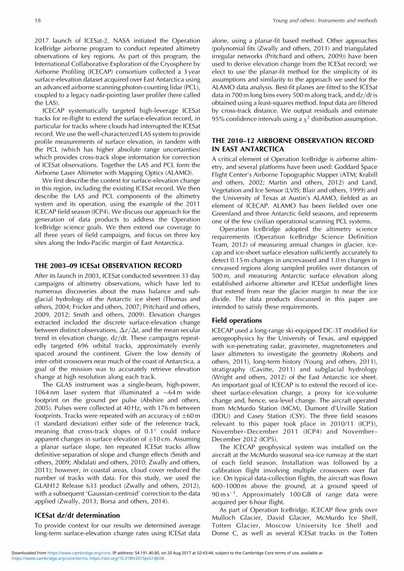
Glacier, David Glacier and Byrd Glacier catchments(Fig. 1). ICECAP also re-flew three ICESat tracks over theunnamed tributary ice streams of the Cook Ice Shelf, whichlie in George V Land overlying deep troughs extending intothe Wilkes Subglacial Basin.

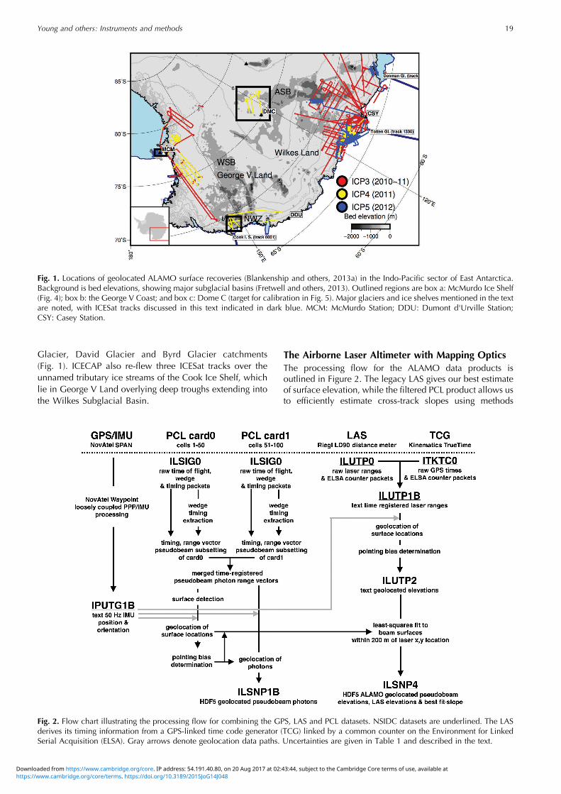
The Airborne Laser Altimeter with Mapping OpticsThe processing flow for the ALAMO data products isoutlined in Figure 2. The legacy LAS gives our best estimateof surface elevation, while the filtered PCL product allows usto efficiently estimate cross-track slopes using methods

Fig. 2. Flow chart illustrating the processing flow for combining the GPS, LAS and PCL datasets. NSIDC datasets are underlined. The LASderives its timing information from a GPS-linked time code generator (TCG) linked by a common counter on the Environment for LinkedSerial Acquisition (ELSA). Gray arrows denote geolocation data paths. Uncertainties are given in Table 1 and described in the text.

Fig. 1. Locations of geolocated ALAMO surface recoveries (Blankenship and others, 2013a) in the Indo-Pacific sector of East Antarctica.Background is bed elevations, showing major subglacial basins (Fretwell and others, 2013). Outlined regions are box a: McMurdo Ice Shelf(Fig. 4); box b: the George V Coast; and box c: Dome C (target for calibration in Fig. 5). Major glaciers and ice shelves mentioned in the textare noted, with ICESat tracks discussed in this text indicated in dark blue. MCM: McMurdo Station; DDU: Dumont d'Urville Station;CSY: Casey Station.

Young and others: Instruments and methods 19





required for ICESat-2. These ALAMO datasets (ILSNP1B andILSNP4), acquired during Operation IceBridge, along withthe input aircraft positioning data (IPUTG1B) and LAS data(ILUPT1B and ILUTP2), are freely available through the USNational Snow and Ice Data Center (NSIDC) and NASA’sReverb data server (Blankenship and others, 2013a,b).The LAS and the PCL share the same inertial measure-

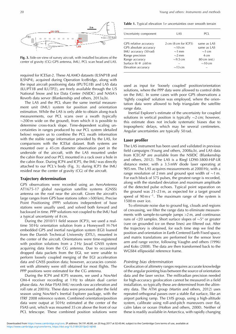
ment unit (IMU) system for position and orientationestimation. While the LAS is only able to obtain along-trackmeasurements, our PCL scans over a swath (typically�200m wide on the ground), from which it is possible todetermine cross-track slope. Time-dependent scaling un-certainties in ranges produced by our PCL system (detailedbelow) require us to combine the PCL swath informationwith the stable range information provided by the LAS, forcomparisons with the ICESat dataset. Both systems aremounted over a 45 cm diameter observation port in theunderside of the aircraft, with the LAS mounted underthe cabin floor and our PCL mounted in a rack over a hole inthe cabin floor. During ICP4 and ICP5, the IMU was directlyattached to our PCL’s body (Fig. 3); during ICP3 the IMUresided near the center of gravity (CG) of the aircraft.

Trajectory determinationGPS observations were recorded using an AeroAntennaAT1675-17 global navigation satellite systems (GNSS)antenna on the roof near the aircraft. Given the aircraft’slarge ranges from GPS base stations (often >500 km), PrecisePoint Positioning (PPP) solutions independent of basestations were usually used, and solved both forward andbackward in time. PPP solutions not coupled to the IMU hada typical uncertainty of 8 cm.During the 2010/11 field season (ICP3), we used a real-

time 50Hz orientation solution from a Honeywell H-764embedded GPS and inertial navigation system (EGI) loanedfrom the Danish Technical University (DTU), mounted inthe center of the aircraft. Orientations were time-registeredwith position solutions from a 2Hz Javad GNSS systemacquiring data from the CG antenna. Due to occasionaldropped data packets from the EGI, we were unable toperform loosely coupled merging of the EGI accelerationdata and GNSS position data; however, accuracies consist-ent with altimetry were still obtained for most flights. ThePPP positions were estimated for the CG antenna.During the ICP4 and ICP5 seasons, we used a NovAtel

OM-4 receiver recording at 1Hz to obtain dual carrierphase data. An iMar FSAS IMU records raw acceleration androll rate at 200Hz. These data were processed after the fieldseason using NovAtel’s Inertial Explorer package, with theITRF 2008 reference system. Combined orientation/positiondata were output at 50Hz estimated at the center of theFSAS unit, which was mounted 35 cm above the front of ourPCL telescope. These combined position solutions were

used as input for ‘loosely coupled’ position/orientationsolutions, where the PPP data were allowed to control driftson the IMU. In some cases with poor GPS observations a‘tightly coupled’ solution was employed, where the orien-tation data were allowed to help triangulate the satelliterange data.Inertial Explorer’s estimate of the uncertainty for coupled

solutions in vertical position is typically �2 cm; however,this estimate does not include systematic biases due totropospheric delays, which may be several centimeters.Angular uncertainties are typically 50 rad.

Laser profilerThe LAS instrument has been used and validated in previousfield campaigns (Young and others, 2008a,b), and LAS datafrom ICECAP are available from the NSIDC (Blankenshipand others, 2012). The LAS is a Riegl LD90-3800-HiP-LRdistance meter, with a 3.5mW diode laser operating at905 nm. The LAS acquires measurements at 2000Hz, with arange resolution of 2mm and ground spot width of �1m.For each block of 575 pulses, the greatest range is recorded,along with the standard deviation and maximum amplitudeof the detected pulse echoes. Typical point separation onthe ground was 21–23m, as expected for a target groundspeed of 90m s� 1. The maximum range of the system is1500m over ice.To eliminate noise due to ground fog, clouds and regions

of crevassing, we filter the range data to eliminate measure-ments with sample-to-sample jumps >2m, and continuousruns of <20 samples. Short surface slopes of �5° or greater(rare on grounded ice on these lines) are filtered out. Afterthe trajectory is obtained, for each time step we find theposition and orientation in Earth Centered Earth Fixed space,and matrix translations are performed for the sensor leverarm and range vector, following Vaughn and others (1996)and Koks (2008). The data are then transformed back to theWGS84 ellipsoidal reference frame.

Pointing bias determinationGeolocation of altimetry ranges requires accurate knowledgeof the angular pointing bias between the source of orientationdata and the laser vector. The milliradian precision neededfor high-accuracy geolocation cannot be measured in a fieldinstallation, so typically these are determined from the altim-etry data. The ATM group (Martin and others, 2012) usesrepeated orthogonal passes over a stable flat surface, like anairport parking ramp. The LVIS group, using a high-altitudesystem, calibrate using roll-and-pitch maneuvers over flat,calm lakes or ocean (Hofton and others, 2000). Neither ofthese is readily available in Antarctica, with rapidly changing

Table 1. Typical elevation 1� uncertainties over smooth terrain

Uncertainty component LAS PCL

GPS relative accuracy 2 cm (8 cm for ICP3) same as LASGPS absolute accuracy �10 cm same as LASIMU accuracy (50 rad) �1mm �1 cmRange precision �2mm 4cmRange accuracy �9.5 cm 80 cm (est.)Surface fit @ �60m – �10 cmElevation accuracy �13 cm –

Fig. 3. Side-on view of survey aircraft, with installed locations of thecenter of gravity (CG) GPS antenna, IMU, PCL scan head and LAS.






skiways or sea-ice infested coastal ocean being normal. Weuse elevation differences at orthogonal line crossovers todetermine our pointing bias, and designed calibration flightsto maximize crossovers of flat targets. We search the roll-bias/pitch-bias space for the minimum root-mean-square(rms) crossover difference. Without accurate a priori data forthe surface, range offsets are hard to determine, and canbleed into pitch-bias determination.On Flight 23 of the ICP4 season, we conducted a gridded

survey of the McMurdo Ice Shelf (Fig. 4). The line spacingwas 2 km� 10 km over an area of 20 km�100 km, yielding100 line crossings. We edited out crossovers over crevassedice; the results of the crossover minimization are detailed inTable 2. Similar calibration surveys were performed in ICP3and ICP5.Due to the bathymetric complexity of the McMurdo

Sound, we did not correct for tides; based on GPSmeasurements on the ice shelf, we expect 8 cm rmsdifference between crossovers due to tides.

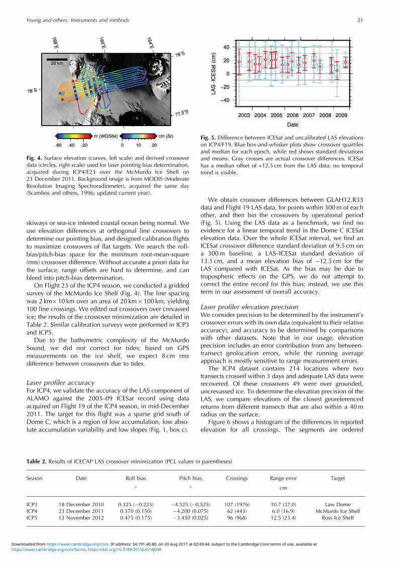
Laser profiler accuracyFor ICP4, we validate the accuracy of the LAS component ofALAMO against the 2003–09 ICESat record using dataacquired on Flight 19 of the ICP4 season, in mid-December2011. The target for this flight was a sparse grid south ofDome C, which is a region of low accumulation, low abso-lute accumulation variability and low slopes (Fig. 1, box c).

We obtain crossover differences between GLAH12.R33data and Flight 19 LAS data, for points within 300m of eachother, and then bin the crossovers by operational period(Fig. 5). Using the LAS data as a benchmark, we find noevidence for a linear temporal trend in the Dome C ICESatelevation data. Over the whole ICESat interval, we find anICESat crossover difference standard deviation of 9.5 cm ona 300m baseline, a LAS–ICESat standard deviation of13.1 cm, and a mean elevation bias of � 12:5 cm for theLAS compared with ICESat. As the bias may be due totropospheric effects on the GPS, we do not attempt tocorrect the entire record for this bias; instead, we use thisterm in our assessment of overall accuracy.

Laser profiler elevation precisionWe consider precision to be determined by the instrument’scrossover errors with its own data (equivalent to their relativeaccuracy), and accuracy to be determined by comparisonswith other datasets. Note that in our usage, elevationprecision includes an error contribution from any between-transect geolocation errors, while the running averageapproach is mostly sensitive to range measurement errors.The ICP4 dataset contains 214 locations where two

transects crossed within 3 days and adequate LAS data wererecovered. Of these crossovers 49 were over grounded,uncrevassed ice. To determine the elevation precision of theLAS, we compare elevations of the closest georeferencedreturns from different transects that are also within a 40mradius on the surface.Figure 6 shows a histogram of the differences in reported

elevation for all crossings. The segments are ordered

Fig. 4. Surface elevation (curves, left scale) and derived crossoverdata (circles, right scale) used for laser pointing bias determination,acquired during ICP4/F23 over the McMurdo Ice Shelf on23 December 2011. Background image is from MODIS (ModerateResolution Imaging Spectroradiometer), acquired the same day(Scambos and others, 1996; updated current year).

Table 2. Results of ICECAP LAS crossover minimization (PCL values in parentheses)

Season Date Roll bias Pitch bias Crossings Range error Target

° ° cm

ICP3 18 December 2010 0.325 (� 0:225) � 4:525 (� 0:525) 107 (1976) 10.7 (37.0) Law DomeICP4 23 December 2011 0.370 (0.150) � 4:200 (0.075) 62 (443) 6.0 (16.9) McMurdo Ice ShelfICP5 13 November 2012 0.475 (0.175) � 3:450 (0.025) 96 (968) 12.5 (23.4) Ross Ice Shelf

Fig. 5. Difference between ICESat and uncalibrated LAS elevationson ICP4/F19. Blue box-and-whisker plots show crossover quartilesand median for each epoch, while red shows standard deviationsand means. Gray crosses are actual crossover differences. ICESathas a median offset of +12.5 cm from the LAS data; no temporaltrend is visible.






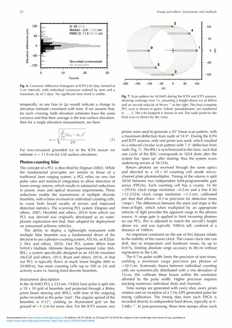
temporally, so any bias in �z would indicate a change inelevation estimate correlated with time. If we assume that,for each crossing, both elevation estimates have the samevariance and that their average is the true surface elevation,then for a single elevation measurement, we have

� ¼

ffiffiffiffiffiffiffiffiffiffiffiffiffiffiffiffiffiffiffiffiffiffiffiffiffiffiffiffiffiffiffiffiffiPN

i¼1ðz2, i � z1, iÞ2

2N

vuuut

ð1Þ

For non-crevassed grounded ice in the ICP4 season weestimate � ¼ 11:9 cm for LAS surface elevations.

Photon-counting lidarThe concept of a PCL is described by Degnan (2002). Whilethe fundamental principles are similar to those of atraditional laser ranging system, a PCL relies on very fastpulse rates and statistical integration to allow detection oflower-energy returns, which results in substantial reductionsin power, mass and optical structure requirements. Thesereductions enable the transmission of multiple discretebeamlets, with echoes received on individual counting cells,to cover both broad swaths of terrain and improveddetection statistics. The scanning PCL system (Degnan andothers, 2007; Herzfeld and others, 2014) from which ourPCL was derived was originally developed as an outer-planets exploration test bed, then adapted for deploymenton unmanned airborne vehicles.The ability to deploy a lightweight instrument with

multiple lidar beamlets was a fundamental driver of thedecision to use a photon-counting system, ATLAS, on ICESat-2 (Wu and others, 2010). Our PCL system differs fromNASA’s Multiple Altimeter Beam Experimental Lidar (MA-BEL), a system specifically designed as an ATLAS simulator(McGill and others, 2013; Brunt and others, 2014), in thatour PCL is typically flown at much lower heights (800 vs20 000m), has more counting cells (up to 100 vs 24) andactively scans vs. having fixed discrete beamlets.

Instrument descriptionIn the ALAMO PCL a 532nm, 19 kHz laser pulse is split intoa 10� 10 grid of beamlets and projected through a Risleyprism beam steering unit (BSU), with time of the outgoingpulse recorded as the pulse ‘start’. The angular spread of thebeamlets is 0.12°, yielding an illuminated grid on theground of �1–2m for every shot. For the ICP3 season, two

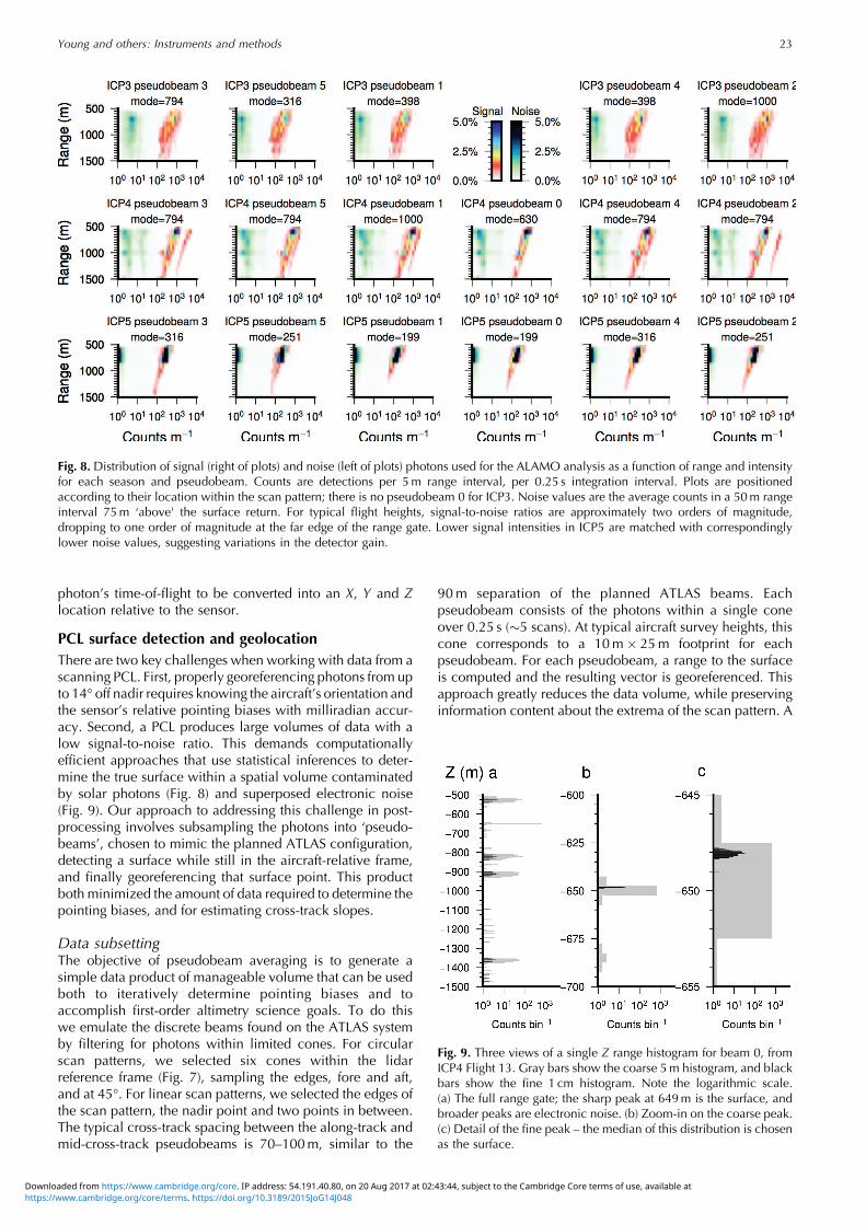
prisms were used to generate a 45° linear scan pattern, witha maximum deflection from nadir of 14.9°. During the ICP4and ICP5 seasons, only one prism was used, which resultedin a reduced circular scan pattern with 7.3° deflection fromnadir (Fig. 7). The BSU is synchronized to the laser, such thatone cycle of the BSU corresponds to 1024 shots after thesystem has ‘spun up’ after starting; thus the system scansunderlying terrain at 18.5Hz.Return photons are received through the same optics

and directed to a 10� 10 counting cell anode micro-channel plate photomultiplier. Timing of the returns is split50/50 between two independent field-programmable gatearrays (FPGAs). Each counting cell has a coarse, 16 bit�295Hz clock (range resolution �0.5m) and a fine 8 bit�12.5GHz clock (range resolution �1.2 cm), calibratedper shot that allows �0.1 ns precision for detection times(‘stops’). The differences between the starts and stops is thetime-of-flight, which when multiplied by an appropriatevelocity of light provides the apparent range to the photonsource. A range gate is applied to limit incoming photonson our PCL; this is adjusted to match the aircraft’s heightabove ice, and was typically 1000m tall, centered at adistance of 1000m.An important constraint on the use of this dataset relates

to the stability of the coarse clock. The coarse clock rate candrift, due to temperature and hardware issues, by up to0.01%, limiting absolute range accuracy to 80 cm withoutregistration to the LAS.The 0.7 ns pulse width limits the precision of start times,

yielding a minimum range precision per photon of�10.5 cm. Systematic biases between individual countingcells are symmetrically distributed with a rms deviation of15 cm. We calibrate these biases within the resolutionafforded by the pulse width. Higher precision requiresstacking numerous individual shots and channels.Time stamps are generated with every shot, every prism

rotation and on reception of a 1Hz GPS generated pulse fortiming calibration. The timing data from each FPGA isrecorded directly to independent hard drives, typically at 4–5MB s� 1. In post-processing, these time stamps allow each

Fig. 7. Scan pattern for ALAMO during the ICP4 and ICP5 seasons,showing coverage over 1 s, assuming a height above ice of 800mand an aircraft velocity of 90m s� 1 to the right. The final completePCL scan is shown in green. Subset ‘pseudobeams’ are numbered0, . . . , 5. The LAS footprint is shown in red. The nadir point for thefinal scan is shown by the cross.

Fig. 6. Crossover difference histogram of ICP4 LAS data, binned at5 cm intervals, with individual crossovers ordered by time and amaximum �t of 3 days. No significant time trend is visible.






photon’s time-of-flight to be converted into an X, Y and Zlocation relative to the sensor.

PCL surface detection and geolocationThere are two key challenges when working with data from ascanning PCL. First, properly georeferencing photons from upto 14° off nadir requires knowing the aircraft’s orientation andthe sensor’s relative pointing biases with milliradian accur-acy. Second, a PCL produces large volumes of data with alow signal-to-noise ratio. This demands computationallyefficient approaches that use statistical inferences to deter-mine the true surface within a spatial volume contaminatedby solar photons (Fig. 8) and superposed electronic noise(Fig. 9). Our approach to addressing this challenge in post-processing involves subsampling the photons into ‘pseudo-beams’, chosen to mimic the planned ATLAS configuration,detecting a surface while still in the aircraft-relative frame,and finally georeferencing that surface point. This productboth minimized the amount of data required to determine thepointing biases, and for estimating cross-track slopes.

Data subsettingThe objective of pseudobeam averaging is to generate asimple data product of manageable volume that can be usedboth to iteratively determine pointing biases and toaccomplish first-order altimetry science goals. To do thiswe emulate the discrete beams found on the ATLAS systemby filtering for photons within limited cones. For circularscan patterns, we selected six cones within the lidarreference frame (Fig. 7), sampling the edges, fore and aft,and at 45°. For linear scan patterns, we selected the edges ofthe scan pattern, the nadir point and two points in between.The typical cross-track spacing between the along-track andmid-cross-track pseudobeams is 70–100m, similar to the

90m separation of the planned ATLAS beams. Eachpseudobeam consists of the photons within a single coneover 0.25 s (�5 scans). At typical aircraft survey heights, thiscone corresponds to a 10m� 25m footprint for eachpseudobeam. For each pseudobeam, a range to the surfaceis computed and the resulting vector is georeferenced. Thisapproach greatly reduces the data volume, while preservinginformation content about the extrema of the scan pattern. A

Fig. 8. Distribution of signal (right of plots) and noise (left of plots) photons used for the ALAMO analysis as a function of range and intensityfor each season and pseudobeam. Counts are detections per 5m range interval, per 0.25 s integration interval. Plots are positionedaccording to their location within the scan pattern; there is no pseudobeam 0 for ICP3. Noise values are the average counts in a 50m rangeinterval 75m ‘above' the surface return. For typical flight heights, signal-to-noise ratios are approximately two orders of magnitude,dropping to one order of magnitude at the far edge of the range gate. Lower signal intensities in ICP5 are matched with correspondinglylower noise values, suggesting variations in the detector gain.

Fig. 9. Three views of a single Z range histogram for beam 0, fromICP4 Flight 13. Gray bars show the coarse 5m histogram, and blackbars show the fine 1 cm histogram. Note the logarithmic scale.(a) The full range gate; the sharp peak at 649m is the surface, andbroader peaks are electronic noise. (b) Zoom-in on the coarse peak.(c) Detail of the fine peak – the median of this distribution is chosenas the surface.






version (Blankenship and others, 2013b) of this dataset (withgeolocated photons) is available from NSIDC.

Surface detectionTo determine the surface location, we extract ranges from thepseudobeam’s subset photon cloud. For each pseudobeam,we first build a histogram along the Z vector of our PCLcoordinate system with 5m (coarse) bin resolution (Fig. 9).The maximum bin is selected as the coarse Z distance. Theaverage of a 10m window centered on 15m is used to assesssolar photon levels. Points where the peak coarse bin count is<50, or the coarse signal-to-noise ratio (SNR) is <2.5 areexcluded from the subsequent analysis. To determine a moreprecise location, we return the median Z distance of photonsin the maximum coarse bin and the two adjacent bins. Giventypical SNRs of 100 (Fig. 8), we estimate the precision of the40 cm wide integrated pulse to be

� ¼�rangeffiffiffiffiffiffiffiffiffiffiSNRp ¼

40 cmffiffiffiffiffiffiffiffiffi100p ¼ 4 cm ð2Þ

Using the known angles for this pseudobeam and thecomputed distance to the surface in the Z-direction, wecalculate X-distance and Y-distance in our PCL’s referenceframe. We then geolocate the surface range vector using themethod used for the LAS system. Photon counts for the peakcoarse and fine bins, the background noise rate, andinformation on the shape of the integrated surface returnare also reported. These data are distributed by NSIDC aspart of Operation IceBridge’s ILSNP4 data (Blankenship andothers, 2013a). Locations of ILSNP4 PCL surface elevationdata in the Wilkes Land region of East Antarctica are shownin Figure 1.

SURFACE-ELEVATION CHANGE DETERMINATIONFor this paper, we use the ILSNP4 slope and elevation dataproduct to assess the linear, invariant component of surface-elevation change over the ICESat record, as constrained bythe ALAMO cross-track slope product. We also use theILSNP4 data to investigate the surface-elevation changesince the end of the ICESat record, for which ICECAPrepresents a unique record.

Slope derivationWe derived surface slope using geolocated PCL beamsurface detections within 200m of each LAS point todetermine a best-fit plane specified by

zðx, yÞ ¼ axþ by þ c ð3Þ

where a, b and c are constants defining the slope, x and yare eastings and northings in the standard polar stereo-graphic projection, and z is elevation in the WGS84coordinate system. z at the location of the LAS coordinateis fixed to the LAS elevation. Solutions that are notconstrained by at least ten points from a side-pointingpseudobeam are rejected, as are solutions where thecentroid of the PCL points is >66m from the LAS spot. Weused a linear least-squares method to perform the fit, andoutput the standard deviation of the residuals, as well as theslope parameters.These combined surface-elevation and slope estimates

are included in the ILSNP4 Hierarchical Data Format 5(HDF5) data product available from NSIDC (Blankenshipand others, 2013a).

Linear ALAMO–ICESat dz/dt determinationUsing the ALAMO slope parameters, we find all ICESat foot-prints within 200m of each LAS spot measurement. We use

bzðxþ �x, yþ �yÞ ¼ zðx, yÞ þ a�xþ b�y ð4Þ

to estimate the ALAMO elevation at each ICESat point, andfind the elevation differences,�zI� A, and the time separation�tI� A, where ‘I’ and ‘A’ indicate ICESat and ALAMO,respectively. We filter out ICESat footprints with�zI� A > 20m, interpreting them as non-physical. For eachLAS spot, we solve

�zI� A ¼ dz=dt�tI� A þ C ð5Þ

as a linear fit to these two vectors, requiring a minimum offour ICESat footprints. dz=dt is the time-invariant rate ofsurface-elevation change, and C is the difference betweenexpected and observed elevations if this trend had continuedto the time of the ALAMO observation. From the residuals weestimate the R2 of the fit and combine the residuals with thenumber of footprints to find the 95% confidence intervalsassuming a �2 distribution. For this analysis, no binning orfiltering of the trends obtained is performed beyond this stepto further elucidate the sources of uncertainty.

Post-ICESat elevation changeC should be equal to zero if linear trends identified abovecontinue to the time of the ICECAP observation. If the 2003–09 dz=dt trend is significant but C is larger than the instru-ment errors, this would imply a change in behavior of thesystem. Where the ICESat era trend is significant, we convertC into the linear rate required to match the end of the ICESattime series to the ALAMO observation using the equation

dzdt2009þ

¼dzdt�

CdtICESat

ð6Þ

where dz/dt is elevation rate of change over the ICESatperiod and dtICESat is the time between the end of the ICESattime series and the ALAMO observation. Propagating the13 cm elevation error we estimate for LAS elevations (theultimate source of ALAMO surface elevations) through thisequation leads to an uncertainty of 7 cm in ICP3 and 3.5 cmin ICP5 due to ALAMO. The bulk of the uncertainty is in thetrend-line estimate of C. We therefore restrict this analysis toICESat era trends with an R2 value of at least 0.8.

RESULTS AND ANALYSISWilkes Land overviewWilkes Land and the adjacent George V Land of the Indo-Pacific sector of the Southern Ocean adjoins a region of theEast Antarctic ice sheet underlain by deep subglacial basinsthat bear evidence of considerable past retreat (Jordan andothers, 2010; Young and others, 2011) and current sub-glacial activity (Smith and others, 2009; Wright and others,2012; McMillan and others, 2013). As these basins aregrounded below sea level and slope toward the interior, theoverlying ice sheet is susceptible to rapid retreat through themarine ice-sheet instability if restraining forces on the sidesand front are released, in particular from bounding iceshelves (Schoof, 2007).Estimates from ice divergence indicate that basal melt

rates are currently low at Cook Ice Shelf (Rignot and others,2013), and evidence of current ice loss from the groundedice inland from spaceborne repeat altimetry (Pritchard and






others, 2009) and gravity (Chen and others, 2009; Luthckeand others, 2013) has been ambiguous.Totten Glacier is one of the largest glaciers on Earth and

has exhibited consistent lowering across the satellite record(Davis and others, 2005; Zwally and others, 2005; Flamentand Rémy, 2012; Khazendar and others, 2013), althoughrough terrain and pervasive cloud cover make it a difficulttarget for radar and optical systems, respectively.Denman Glacier represents another outlet of the Aurora

Subglacial |Basin, and from satellite data has also exhibitedlowering trends, associated with a dynamical ice shelf.However, due to its location in a pronounced valley in theice sheet, and association with exposed nunataks and blue-ice regions, it has been hypothesized that the lowering maybe due to enhanced wind erosion (Flament andRémy, 2012).

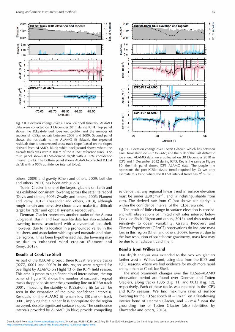
Results at Cook Ice ShelfAs part of the ICECAP project, three ICESat reference tracks(0277, 0001 and 0039) in this region were targeted foroverflight by ALAMO on Flight 13 of the ICP4 field season.This area is prone to significant cloud interruptions; the toppanel of Figure 10 shows the number of successful repeattracks dropped to six near the grounding line on ICESat track0001, impacting the stability of ICESat-only fits (as can beseen in the expansion of the pink confidence intervals).Residuals for the ALAMO fit remain low (30 cm) on track0001, implying that a planar fit is appropriate for the regionsurveyed, despite significant surface slopes. The confidenceintervals provided by ALAMO (in blue) provide compelling

evidence that any regional linear trend in surface elevationmust be under �30 cma� 1, and is indistinguishable fromzero. The derived rate from C (not shown for clarity) iswithin the confidence interval of the ICESat era rate.The result of little change in surface elevation is consist-

ent with observations of limited melt rates inferred belowCook Ice Shelf (Rignot and others, 2013), and thus reducedsensitivity to ocean variability. Gravity Recovery andClimate Experiment (GRACE) observations do indicate massloss in this region (Chen and others, 2009); however, due tothe low resolution of spaceborne gravimetry, mass loss maybe due to an adjacent catchment.

Results from Wilkes LandOur dz=dt analysis was extended to the two key glaciersfurther west in Wilkes Land, using data from the ICP3 andICP5 seasons, where we find evidence for much more rapidchange than at Cook Ice Shelf.The most prominent changes over the ICESat–ALAMO

observation period are found over Denman and TottenGlaciers, along tracks 1335 (Fig. 11) and 0033 (Fig. 12),respectively. Each of these tracks was repeated in the ICP3and ICP5 seasons. We find maximum rates of surfacelowering for the ICESat epoch of � 1ma� 1 on a fast-flowinginterior bend of Denman Glacier, and � 2ma� 1 near thegrounding line of Totten Glacier (also identified byKhazendar and others, 2013).

Fig. 10. Elevation change over a Cook Ice Shelf tributary. ALAMOdata were collected on 3 December 2011 during ICP4. Top panelshows the ICESat-derived ice-sheet profile, and the number ofsuccessful ICESat repeats between 2003 and 2009. Second panelshows the residuals to the ALAMO fit (black), the expectedresiduals due to uncorrected cross-track slope (based on the slopesderived from ALAMO, blue); white background shows where theaircraft track was within 100m of the ICESat reference track. Thethird panel shows ICESat-derived dz=dt with a 95% confidenceinterval (pink). The bottom panel shows ALAMO-corrected ICESatdz=dt with a 95% confidence interval (blue).

Fig. 11. Elevation change over Totten Glacier, which lies betweenLaw Dome (latitude � 67 to � 66�) and the bulk of the East Antarcticice sheet. ALAMO data were collected on 30 December 2010 inICP3 and 1 December 2012 during ICP5. Key is the same as Figure10; the fifth panel shows ICP3 ALAMO data. The purple linerepresents the post-ICESat dz=dt trend required by C; we onlyestimate this trend where the ICESat interval trend has R2 > 0:8.






Totten GlacierIn both the ICESat-only case (pink in Fig. 11 third panel)and the ALAMO-corrected datasets the hypothesis of nolinear trend can be rejected, with confidence intervals of�25 cm for most of the region. One region where theplanar assumption used for both ICESat-only and ALAMOdatasets appears to degrade is the south side and summit ofLaw Dome. This region of Law Dome is dominated by blueice and steep ice slopes; increased residuals (and acorresponding increase in the size of the confidenceinterval) are apparent.For Totten Glacier, we find in general that the difference

in ICESat and post-ICESat trends is within the 95%confidence interval, implying no significant changes inlowering. An exception is linked to a 5 km wide prominentspike of surface-elevation growth during the ICESat era at� 67:8°, focused on a downstream stepping 200m bedrelief feature. This feature may represent a localizedsubglacial hydraulic feature with time-varying behavior,and is linked to the interior subglacial hydrological network(Wright and others, 2012).

Denman GlacierTrack 0033 (Fig. 12) samples a variety of different terrains inWilkes Land, including the Obruchev Hills, a complex ofnunataks and blue ice on the ice-sheet slope, marginal icefeeding the main trunk of Denman Glacier (between � 66:6and � 66:95°), and the shear margin of Denman Glacier. It isalso in a cloudy portion of the Antarctic coast, with <10

repeats available for ICESat analysis. We find (as expected)very high residuals over the Obruchev Hills, and also whilecrossing the shear margin of Denman Glacier. We find in themarginal ice a progressive increasing lowering rate from� 50 cma� 1 to � 1ma� 1 as the shear margin is approached.When examining the implied post-ICESat rates (purple curvesin Fig. 12), we find that rates over the shear margin of theglacier appear to have doubled. These observations would beconsistent with a slowing of the main glacier trunk, followedby a kinematic wave propagating upstream.

CONCLUSIONSDuring the course of NASA’s Operation IceBridge, ICECAPcollected 25039 track kilometers of re-flights of ICESat linesover the margins of the East Antarctic ice sheet. TheAirborne Laser Altimeter with Mapping Optics (ALAMO), ascanning photon-counting lidar registered to a nadir laserprofiler, was deployed to extend the elevation record ofICESat. We find the ALAMO dataset meets IceBridge sciencerequirements and can confirm and enhance the ICESatrecord in Antarctica.With our record along existing ICESat lines we find little

evidence of broad surface-elevation change in the regionfeeding Cook Ice Shelf, indicating a relatively stable systemthere. Conversely, our observations show continued dra-matic ice lowering at Denman and Totten Glaciers, likelydriven by changes in the floating portions of the glacierscaused by enhanced ice-shelf melting. We also findevidence of localized surface-elevation change, consistentwith subglacial hydrology. This paper represents the firstdemonstration of swath photon-counting altimetry overAntarctica and sets a precedent for ATLAS observationsover ice sheets following the launch of ICESat-2.

ACKNOWLEDGEMENTSFunding for the fieldwork and data reduction was providedby NASA grants NNX09AR52G, NNG10HP06C andNNX11AD33G, Program DACOTA (06-VULN-016) of theAgence Nationale pour la Recherche, and UK NaturalEnvironment Research Council grant NE/D003733/1. Thiswork was supported by the Australian Government’sCooperative Research Centres Programme through theAntarctic Climate and Ecosystems Cooperative ResearchCentre (ACE CRC). This work received funding from theAmerican Recovery and Reinvestment Act. Logistical sup-port was provided by Australian Antarctic Division (throughAustralian Antarctic Programme projects 3103 and 4077),the US Antarctic Program and the French Polar Institute. Wethank DTU for their loan of an EGI and thank Gabriel Jodorand Christopher Field of Simga Space Corporation fortechnical guidance with this system. We thank Chad Greenefor reviewing drafts of this paper, and Tom Neumann, ananonymous reviewer and the scientific editor, Helen Fricker,for valuable suggestions. This paper is UTIG contributionNo. 2699.

REFERENCESAbdalati W and 16 others (2010) The ICESat-2 laser altimetrymission. IEEE Proc., 98(5), 735–751 (doi: 10.1109/JPROC.2009.2034765)

Fig. 12. Elevation change over the edge of Denman Glacier,between the Obruchev Hills (� 66:6° to � 66:5°) and the shearmargin of Denman Glacier (south of � 67°). ALAMO data werecollected on 18 January 2011 during ICP3 and 30 November 2012during ICP5. Key is the same as Figure 10; the bottom panel showsICP3 ALAMO data.






Abshire JB and 7 others (2005) Geoscience Laser Altimeter System(GLAS) on the ICESat Mission: on-orbit measurement perform-ance. Geophys. Res. Lett., 32(21), L21S02 (doi: 10.1029/2005GL024028)

Blair JB, Rabine DL and Hofton MA (1999) The Laser VegetationImaging Sensor: a medium-altitude, digitisation-only, airbornelaser altimeter for mapping vegetation and topography. ISPRS J.Photogramm. Remote Sens., 54(2–3), 115–122 (doi: 10.1016/S0924-2716(99)00002-7)

Blankenship DD, Kempf SD and Young DA (2012) IceBridge RieglLaser Altimeter L2 Geolocated Surface Elevation Triplets [EastAntarctica]. NASA Distributed Active Archive Center, NationalSnow and Ice Data Center, Boulder, CO. Digital media: http://nsidc.org/data/ilutp2 (updated 2013)

Blankenship DD, Kempf SD, Young DA and Lindzey LE (2013a)IceBridge Merged Photon Counting Lidar/Profiler L4 SurfaceSlope and Elevations [East Antarctica]. NASA Distributed ActiveArchive Center, National Snow and Ice Data Center, Boulder,CO. Digital media: http://nsidc.org/data/ilsnp4

Blankenship DD, Kempf SD, Young DA and Lindzey LE (2013b)IceBridge Photon Counting Lidar L1B Subset Geolocated PhotonElevations [East Antarctica]. NASA Distributed Active ArchiveCenter, National Snow and Ice Data Center, Boulder, CO.(updated 2014) Digital media: http://nsidc.org/data/ilutp2

Borsa AA, Moholdt G, Fricker HA and Brunt KM (2014) A rangecorrection for ICESat and its potential impact on ice-sheet massbalance studies. Cryosphere, 8(2), 345–357 (doi: 10.5194/tc-8-345-2014)

Brunt KM, Neumann TA, Walsh KM and Markus T (2014)Determination of local slope on the Greenland Ice Sheet usinga multibeam photon-counting Lidar in preparation for theICESat-2 Mission. IEEE Geosci. Remote Sens. Lett., 11(5),935–939 (doi: 10.1109/LGRS.2013.2282217)

Cavitte M (2011) Using radio-echo sounding as a tool forcorrelating ice core ages between Dome C and Vostok, EastAntarctica. (MSc thesis, University of Cambridge)

Chen JL, Wilson CR, Blankenship D and Tapley BD (2009)Accelerated Antarctic ice loss from satellite gravity measure-ments. Nature Geosci., 2(12), 859–862 (doi: 10.1038/ngeo694)

Church JA and 13 others (2013) Sea level change. In Stocker TF and9 others eds. Climate change 2013: the physical science basis.Contribution of Working Group I to the Fifth Assessment Reportof the Intergovernmental Panel on Climate Change. CambridgeUniversity Press, Cambridge

Davis CH, Li Y, McConnell JR, Frey MM and Hanna E (2005)Snowfall-driven growth in East Antarctic ice sheet mitigatesrecent sea-level rise. Science, 308(5730), 1898–1901 (doi:10.1126/science.1110662)

Degnan JJ (2002) Photon-counting multikilohertz microlaseraltimeters for airborne and spaceborne topographic measure-ments. J. Geodyn., 34(3–4), 503–549 (doi: 10.1016/S0264-3707(02)00045-5)

Degnan J, Wells D, Machan R and Leventhal E (2007) Secondgeneration airborne 3D imaging lidars based on photoncounting. In Becker W ed. Advanced photon counting tech-niques II. (Proceedings of SPIE 6771) International Society forOptics and Photonics, Bellingham, WA

Flament T and Rémy F (2012) Dynamic thinning of Antarcticglaciers from along-track repeat radar altimetry. J. Glaciol.,58(211), 830–840 (doi: 10.3189/2012JoG11J118)

Flament T, Berthier E and Rémy F (2014) Cascading waterunderneath Wilkes Land, East Antarctic Ice Sheet, observedusing altimetry and digital elevation models. Cryosphere, 8(2),673–687 (doi: 10.5194/tc-8-673-2014)

Fretwell P and 59 others (2013) Bedmap2: improved ice bed,surface and thickness datasets for Antarctica. Cryosphere, 7(1),375–393 (doi: 10.5194/tc-7-375-2013)

Fricker HA, Scambos T, Bindschadler R and Padman L (2007) Anactive subglacial water system in West Antarctica mapped

from space. Science, 315(5818), 1544–1548 (doi: 10.1126/science.1136897)

Herzfeld UC and 6 others (2014) Algorithm for detection of groundand canopy cover in micropulse photon-counting lidar altimeterdata in preparation for the ICESat-2 Mission. IEEE Trans. Geosci.Remote Sens., 52(4), 2109–2125 (doi: 10.1109/TGRS.2013.2258350)

Hofton M and 6 others (2000) An airborne laser altimetry survey ofLong Valley, California. Int. J. Remote Sens., 21(12), 2413–2437(doi: 10.1080/01431160050030547)

Intergovernmental Panel on Climate Change (IPCC) (2013) Summaryfor policymakers. In Stocker TF and 9 others eds. Climate change2013: the physical science basis. Contribution of Working GroupI to the Fifth Assessment Report of the Intergovernmental Panel onClimate Change. Cambridge University Press, Cambridge

Jordan TA, Ferraccioli F, Corr H, Graham A, Armadillo E and BozzoE (2010) Hypothesis for mega-outburst flooding from a palaeo-subglacial lake beneath the East Antarctic Ice Sheet. Terra Nova,22(4), 283–289 (doi: 10.1111/j.1365-3121.2010.00944.x)

Khazendar A, Schodlok MP, Fenty I, Ligtenberg SRM, Rignot E andVan den Broeke MR (2013) Observed thinning of Totten Glacieris linked to coastal polynya variability. Nature Commun., 4 (doi:10.1038/ncomms3857)

Koks D (2008) Using rotations to build aerospace coordinate sys-tems. (Tech. Rep. DSTO-TN-0640) Defence Science andTechnology Organisation Systems Sciences Laboratory, Edin-burgh, Australia

Krabill WB and 8 others (2002) Aircraft laser altimetry measure-ment of elevation changes of the Greenland ice sheet: techniqueand accuracy assessment. J. Geodyn., 34(3–4), 357–376 (doi:10.1016/S0264-3707(02)00040-6)

Luthcke SB, Sabaka TJ, Loomis BD, Arendt A, McCarthy JJ andCamp J (2013) Antarctica, Greenland and Gulf of Alaska land-ice evolution from an iterated GRACE global mascon solution.J. Glaciol., 59(216), 613–631 (doi: 10.3189/2013JoG12J147)

Martin CF and 6 others (2012) Airborne topographic mappercalibration procedures and accuracy assessment. (ASA Tech.Rep. NASA/TM-2012-215891) NASA Goddard Space FlightCenter, Greenbelt, MD

McGill M, Markus T, Scott VS and Neumann T (2013) The MultipleAltimeter Beam Experimental Lidar (MABEL): an airbornesimulator for the ICESat-2 Mission. J. Atmos. Ocean. Technol.,30(2), 345–352 (doi: 10.1175/JTECH-D-12-00076.1)

McMillan M, Corr H, Shepherd A, Ridout A, Laxon S and Cullen R(2013) Three-dimensional mapping by CryoSat-2 of subglaciallake volume changes. Geophys. Res. Lett., 40(16), 4321–4327(doi: 10.1002/grl.50689)

McMillan M and 7 others (2014) Increased ice losses fromAntarctica detected by CryoSat-2. Geophys. Res. Lett., 41(11),3899–3905 (doi: 10.1002/2014GL060111)

Operation IceBridge Science Definition Team (2012) IceBridgescience requirements summary. NASA Distributed ActiveArchive Center, National Snow and Ice Data Center, Boulder,CO http://bprc.osu.edu/rsl/IST/index_files/PROJECTDOCU-MENTS.htm

Pritchard HD, Arthern RJ, Vaughan DG and Edwards LA (2009)Extensive dynamic thinning on the margins of the Greenlandand Antarctic ice sheets. Nature, 461(7266), 971–975 (doi:10.1038/nature08471)

Pritchard HD, Ligtenberg SRM, Fricker HA, Vaughan DG, Van denBroeke MR and Padman L (2012) Antarctic ice-sheet loss drivenby basal melting of ice shelves. Nature, 484(7395), 502–505(doi: 10.1038/nature10968)

Rignot E, Jacobs S, Mouginot J and Scheuchl B (2013) Ice shelfmelting around Antarctica. Science, 341(6143), 266–270 (doi:10.1126/science.1235798)

Roberts JL and 12 others (2011) Refined broad-scale sub-glacialmorphology of Aurora Subglacial Basin, East Antarctica derivedby an ice-dynamics-based interpolation scheme. Cryosphere,5(3), 551–560 (doi: 10.5194/tc-5-551-2011)






Scambos T, Bohlander J and Raup B (1996) Images of Antarctic iceshelves [2002–present]. National Snow and Ice Data Center,Boulder, CO. Digital media: http://nsidc.org/data/iceshelves_images/index_modis.html

Schoof C (2007) Ice sheet grounding line dynamics: steady states,stability, and hysteresis. J. Geophys. Res., 112(F3), F03S28 (doi:10.1029/2006JF000664)

Schutz BE, Zwally HJ, Shuman CA, Hancock D and DiMarzio JP(2005) Overview of the ICESat Mission. Geophys. Res. Lett.,32(21), L21S01 (doi: 10.1029/2005GL024009)

Siegfried MR, Fricker HA, Roberts M, Scambos TA and Tulaczyk S(2014) A decade of West Antarctic subglacial lake interactionsfrom combined ICESat and CryoSat-2 altimetry. Geophys. Res.Lett., 41(3), 891–898 (doi: 10.1002/2013GL058616)

Smith BE, Fricker HA, Joughin IR and Tulaczyk S (2009) Aninventory of active subglacial lakes in Antarctica detected byICESat (2003–2008). J. Glaciol., 55(192), 573–595 (doi:10.3189/002214309789470879)

Thomas R and 17 others (2004) Accelerated sea-level rise fromWest Antarctica. Science, 306(5694), 255–258 (doi: 10.1126/science.1099650)

Vaughan DG and 13 others (2013) Observations: cryosphere. InStocker TF and 9 others eds. Climate change 2013: the physicalscience basis. Contribution of Working Group I to the FifthAssessment Report of the Intergovernmental Panel on ClimateChange. Cambridge University Press, Cambridge and New York

Vaughn CR, Bufton JL, Krabill WB and Rabine DL (1996)Georeferencing of airborne laser altimeter measurements.Int. J. Remote Sens., 17(11), 2185–2200 (doi: 10.1080/01431169608948765)

Wouters B, Bamber JL, Van den Broeke MR, Lenaerts JTM andSasgen I (2013) Limits in detecting acceleration of ice sheet massloss due to climate variability. Nature Geosci., 6(8), 613–616(doi: 10.1038/ngeo1874)

Wright AP and 12 others (2012) Evidence of a hydrologicalconnection between the ice divide and ice sheet margin in theAurora Subglacial Basin, East Antarctica. J. Geophys. Res.,117(F1), F01033 (doi: 10.1029/2011JF002066)

Wu AY and 9 others (2010) Space laser transmitter development forICESat-2 mission. SPIE Proc., 7578 (doi: 10.1117/12.843342)

Young DA, Kempf SD, Blankenship DD, Holt JW and Morse DL(2008a) Airborne laser altimetry of the Thwaites Glacier catch-ment, West Antarctica. National Snow and Ice Data Center,Boulder, CO. Digital media: http://nsidc.org/data/nsidc-0334

Young DA, Kempf SD, Blankenship DD, Holt JW and Morse DL(2008b) New airborne laser altimetry over the Thwaites Glaciercatchment, West Antarctica. Geochem. Geophys. Geosyst.,9(Q6), Q06006 (doi: 10.1029/2007GC001935)

Young DA and 11 others (2011) A dynamic early East Antarctic IceSheet suggested by ice-covered fjord landscapes. Nature,474(7349), 72–75 (doi: 10.1038/nature10114)

Zwally HJ (2013) GLAS Release 34 Altimetry: correction to theICESat data product surface elevations due to an error in therange determination from transmit-pulse reference-point selec-tion (centroid vs Gaussian). NASA/Distributed Active ArchiveCenter, National Snow and Ice Data Center, Boulder, CO nsidc.org/data/icesat/correction-to-product-surface-elevations.html

Zwally HJ and 7 others (2005) Mass changes of the Greenland andAntarctic ice sheets and shelves and contributions to sea-levelrise: 1992–2002. J. Glaciol., 51(175), 509–527 (doi: 10.3189/172756505781829007)

Zwally HJ and 11 others (2011) Greenland ice sheet mass balance:distribution of increased mass loss with climate warming; 2003–07 versus 1992–2002. J. Glaciol., 57(201), 88–102 (doi:10.3189/002214311795306682)

Zwally HJ and 7 others (2012) GLAS/ICESat L2 Antarctic andGreenland Ice Sheet altimetry data, version 001 [East Ant-arctica]. National Snow and Ice Data Center, Boulder, CO

MS received 25 March 2014 and accepted in revised form 18 September 2014






land-ice elevation changes from photon-counting swath ... · instruments and methods land-ice...

Documents