land mobile radio transceiver performance recommendations ... · pdf fileland mobile radio...

TIA-102.CAAB-C (Revision of TIA-102.CAAB)

January 2010

Land Mobile Radio Transceiver Performance Recommendations Project 25 - Digital Radio Technology C4FM/CQPSK Modulation

ANSI/TIA-102.CAAB-C APPROVED: JANUARY 8, 2010

--```,``,,`,,``,```,`````,`````-`-`,,`,,`,`,,`---

NOTICE TIA Engineering Standards and Publications are designed to serve the public interest through eliminating misunderstandings between manufacturers and purchasers, facilitating interchangeability and improvement of products, and assisting the purchaser in selecting and obtaining with minimum delay the proper product for their particular need. The existence of such Standards and Publications shall not in any respect preclude any member or non-member of TIA from manufacturing or selling products not conforming to such Standards and Publications. Neither shall the existence of such Standards and Publications preclude their voluntary use by Non-TIA members, either domestically or internationally. Standards and Publications are adopted by TIA in accordance with the American National Standards Institute (ANSI) patent policy. By such action, TIA does not assume any liability to any patent owner, nor does it assume any obligation whatever to parties adopting the Standard or Publication. This Standard does not purport to address all safety problems associated with its use or all applicable regulatory requirements. It is the responsibility of the user of this Standard to establish appropriate safety and health practices and to determine the applicability of regulatory limitations before its use. (From Standards Proposal No. 3-4613-RV3, formulated under the cognizance of the TIA, TR-8 Mobile and Personal Private Radio Standards. TR-8.6 Subcommittee on Equipment Performance Recommendation).

Published by

©TELECOMMUNICATIONS INDUSTRY ASSOCIATION Standards and Technology Department 2500 Wilson Boulevard Arlington, VA 22201 U.S.A.

PRICE: Please refer to current Catalog of TIA TELECOMMUNICATIONS INDUSTRY ASSOCIATION STANDARDS

AND ENGINEERING PUBLICATIONS or call IHS USA and Canada

(1-800-525-7052 ) International (303-790-0600) or search online at http://www.tiaonline.org/standards/catalog/

All rights reserved Printed in U.S.A.

--```,``,,`,,``,```,`````,`````-`-`,,`,,`,`,,`---

--```,``,,`,,``,```,`````,`````-`-`,,`,,`,`,,`---

NOTICE OF DISCLAIMER AND LIMITATION OF LIABILITY

The document to which this Notice is affixed (the “Document”) has been prepared by one or more Engineering Committees or Formulating Groups of the Telecommunications Industry Association (“TIA”). TIA is not the author of the Document contents, but publishes and claims copyright to the Document pursuant to licenses and permission granted by the authors of the contents.

TIA Engineering Committees and Formulating Groups are expected to conduct their affairs in accordance with the TIA Engineering Manual (“Manual”), the current and predecessor versions of which are available at http://www.tiaonline.org/standards/procedures/manuals/TIA’s function is to administer the process, but not the content, of document preparation in accordance with the Manual and, when appropriate, the policies and procedures of the American National Standards Institute (“ANSI”). TIA does not evaluate, test, verify or investigate the information, accuracy, soundness, or credibility of the contents of the Document. In publishing the Document, TIA disclaims any undertaking to perform any duty owed to or for anyone.

If the Document is identified or marked as a project number (PN) document, or as a standards proposal (SP) document, persons or parties reading or in any way interested in the Document are cautioned that: (a) the Document is a proposal; (b) there is no assurance that the Document will be approved by any Committee of TIA or any other body in its present or any other form; (c) the Document may be amended, modified or changed in the standards development or any editing process.

The use or practice of contents of this Document may involve the use of intellectual property rights (“IPR”), including pending or issued patents, or copyrights, owned by one or more parties. TIA makes no search or investigation for IPR. When IPR consisting of patents and published pending patent applications are claimed and called to TIA’s attention, a statement from the holder thereof is requested, all in accordance with the Manual. TIA takes no position with reference to, and disclaims any obligation to investigate or inquire into, the scope or validity of any claims of IPR. TIA will neither be a party to discussions of any licensing terms or conditions, which are instead left to the parties involved, nor will TIA opine or judge whether proposed licensing terms or conditions are reasonable or non-discriminatory. TIA does not warrant or represent that procedures or practices suggested or provided in the Manual have been complied with as respects the Document or its contents.

If the Document contains one or more Normative References to a document published by another organization (“other SSO”) engaged in the formulation, development or publication of standards (whether designated as a standard, specification, recommendation or otherwise), whether such reference consists of mandatory, alternate or optional elements (as defined in the TIA Engineering Manual, 4th edition) then (i) TIA disclaims any duty or obligation to search or investigate the records of any other SSO for IPR or letters of assurance relating to any such Normative Reference; (ii) TIA’s policy of encouragement of voluntary disclosure (see Engineering Manual Section 6.5.1) of Essential Patent(s) and published pending patent applications shall apply; and (iii) Information as to claims of IPR in the records or publications of the other SSO shall not constitute identification to TIA of a claim of Essential Patent(s) or published pending patent applications.

TIA does not enforce or monitor compliance with the contents of the Document. TIA does not certify, inspect, test or otherwise investigate products, designs or services or any claims of compliance with the contents of the Document.

ALL WARRANTIES, EXPRESS OR IMPLIED, ARE DISCLAIMED, INCLUDING WITHOUT LIMITATION, ANY AND ALL WARRANTIES CONCERNING THE ACCURACY OF THE CONTENTS, ITS FITNESS OR APPROPRIATENESS FOR A PARTICULAR PURPOSE OR USE, ITS MERCHANTABILITY AND ITS NONINFRINGEMENT OF ANY THIRD PARTY’S INTELLECTUAL PROPERTY RIGHTS. TIA EXPRESSLY DISCLAIMS ANY AND ALL RESPONSIBILITIES FOR THE ACCURACY OF THE CONTENTS AND MAKES NO REPRESENTATIONS OR WARRANTIES REGARDING THE CONTENT’S COMPLIANCE WITH ANY APPLICABLE STATUTE, RULE OR REGULATION, OR THE SAFETY OR HEALTH EFFECTS OF THE CONTENTS OR ANY PRODUCT OR SERVICE REFERRED TO IN THE DOCUMENT OR PRODUCED OR RENDERED TO COMPLY WITH THE CONTENTS.

--```,``,,`,,``,```,`````,`````-`-`,,`,,`,`,,`---

TIA SHALL NOT BE LIABLE FOR ANY AND ALL DAMAGES, DIRECT OR INDIRECT, ARISING FROM OR RELATING TO ANY USE OF THE CONTENTS CONTAINED HEREIN, INCLUDING WITHOUT LIMITATION ANY AND ALL INDIRECT, SPECIAL, INCIDENTAL OR CONSEQUENTIAL DAMAGES (INCLUDING DAMAGES FOR LOSS OF BUSINESS, LOSS OF PROFITS, LITIGATION, OR THE LIKE), WHETHER BASED UPON BREACH OF CONTRACT, BREACH OF WARRANTY, TORT (INCLUDING NEGLIGENCE), PRODUCT LIABILITY OR OTHERWISE, EVEN IF ADVISED OF THE POSSIBILITY OF SUCH DAMAGES. THE FOREGOING NEGATION OF DAMAGES IS A FUNDAMENTAL ELEMENT OF THE USE OF THE CONTENTS HEREOF, AND THESE CONTENTS WOULD NOT BE PUBLISHED BY TIA WITHOUT SUCH LIMITATIONS.

TIA-102.CAAB-C

i

FOREWORD (This foreword is not part of this Standard) This Standard was developed and will be maintained by the TR-8.6 Equipment Performance Recommendations Subcommittee of the TR-8 Land Mobile Services Committee. Participating in its development were radio equipment and measuring instrument manufacturers as well as representatives of public safety user groups from the Association of Public Safety Communications Officials, International (APCO), the National Association of State Telecommunications Directors (NASTD), and numerous federal government agencies. These user groups and agencies worked together under APCO Project 25, and several subcommittees and working groups at the Telecommunications Industry Association (TIA) worked together with them to formulate a family of Standards and Bulletins. Telecommunications Systems Bulletin TIA TSB-102-A, Project 25 System and Standards Definition, provides an overview of Project 25, outlines the user group requirements, and lists the family of more than 30 TIA documents developed under Project 25 which was intended to provide interoperable digitally modulated radio equipment for public safety users. This standard provides the standard limit values for the equipment characteristics assessed by the measurement methods described in ANSI/TIA-102.CAAA-C, Digital C4FM/CQPSK Transceiver Measurement Methods. This revision of the Standard incorporates equipment performance characteristics for test methods that utilize standard simulcast modulation types as defined in ANSI/TIA-102.CAAA-C, Digital C4FM/CQPSK Transceiver Measurement Methods. This Standard was approved for publication during the October 19, 2009 meeting of Subcommittee TR 8.6. When published it cancels and replaces predecessor document ANSI/TIA102.CAAB-B (July, 2004) There are two annexes in this Standard, The annexes, A and B, are informative and are not considered part of this Standard.

--```,``,,`,,``,```,`````,`````-`-`,,`,,`,`,,`---

TIA-102.CAAB-C

ii

Table of Contents

1 Introduction ............................................................................................................1

1.1 Scope .......................................................................................................................1 1.2 Object .......................................................................................................................1 1.3 Standard Definitions .................................................................................................1 1.4 Standard Test Conditions.........................................................................................1 1.5 Characteristics of Test Equipment ...........................................................................2 1.6 Normative Reference Documents ............................................................................2 1.7 Revision History .......................................................................................................2

2 Methods of Measurements ....................................................................................2

3 Standards for all equipment..................................................................................2

3.1 Receiver Section ......................................................................................................4 3.1.1 Radiated Spurious Field Strength ............................................................................4 3.1.2 Conducted Spurious Output Power..........................................................................4 3.1.3 Power Line Conducted Spurious Output Voltage.....................................................4 3.1.4 Reference Sensitivity................................................................................................5 3.1.5 Faded Reference Sensitivity ....................................................................................5 3.1.6 Signal Delay Spread Capability................................................................................5 3.1.7 Adjacent Channel Rejection .....................................................................................6 3.1.8 Co-Channel Rejection ..............................................................................................6 3.1.9 Spurious Response Rejection ..................................................................................6 3.1.10 Intermodulation Rejection.........................................................................................7 3.1.11 Signal Displacement Bandwidth...............................................................................7 3.1.12 Audio Output Distortion ............................................................................................7 3.1.13 Residual Audio Noise Ratio......................................................................................7 3.1.14 Average Radiation Sensitivity...................................................................................7 3.1.15 Acoustic Audio Output..............................................................................................8 3.1.16 Bit Error Rate Floor ..................................................................................................8 3.1.17 Late Entry Unsquelch Delay.....................................................................................8 3.1.18 Receiver Throughput Delay......................................................................................9 3.2 Transmitter Section ................................................................................................10 3.2.1 RF Output Power....................................................................................................10 3.2.2 Operating Frequency Accuracy..............................................................................10 3.2.3 Electrical Audio Performance .................................................................................11 3.2.4 Acoustic Audio Performance ..................................................................................11 3.2.5 Modulation Emission Spectrum..............................................................................11 3.2.6 Unwanted Emissions: Radiated Spurious ..............................................................12 3.2.7 Unwanted Emissions: Conducted Spurious ...........................................................13 3.2.8 Unwanted Emissions: Non-Spurious Adjacent Channel Power Ratio....................13 3.2.9 Intermodulation Attenuation ...................................................................................14

--```,``,,`,,``,```,`````,`````-`-`,,`,,`,`,,`---

TIA-102.CAAB-C

iii

3.2.10 Radiated Power Output ..........................................................................................15 3.2.11 Conducted Spurious Emissions into VSWR...........................................................16 3.2.12 Transmitter Power and Encoder Attack Time.........................................................16 3.2.13 Transmitter Power and Encoder Attack Time with Busy/Idle Operation.................16 3.2.14 Transmitter Throughput Delay................................................................................16 3.2.15 Frequency Deviation for C4FM ..............................................................................16 3.2.16 Modulation Fidelity .................................................................................................17 3.2.17 Symbol Rate Accuracy ...........................................................................................17 3.2.18 Transient Frequency Behavior ...............................................................................18 3.2.19 RFSS Throughput Delay ........................................................................................19 3.2.20 RFSS Idle to Busy Transition Time ........................................................................20 3.3 Trunked System Timing Characteristics.................................................................21 3.3.1 Trunking Control Channel Slot Times ....................................................................21 3.3.2 Trunking Request Time ..........................................................................................21 3.3.3 Trunking Voice Channel Access Time ...................................................................21 3.3.4 Time to Grant .........................................................................................................22 3.3.5 Transmitter Time to Key on a Traffic Channel........................................................22 3.4 Unit Characteristics ................................................................................................23 3.4.1 Power Supply Voltage Range ................................................................................23 3.4.2 Temperature Range ...............................................................................................25 3.4.3 High Humidity .........................................................................................................26 3.4.4 Vibration Stability....................................................................................................27 3.4.5 Shock Stability........................................................................................................27 3.4.6 DC Supply Noise Susceptibility ..............................................................................28 3.4.7 Battery Life .............................................................................................................28 3.4.8 Dimensions.............................................................................................................29 3.4.9 Weight ....................................................................................................................29 3.4.10 Other Environmental ..............................................................................................29

ANNEX A Measurement Uncertainty (Informative).............................................................33

A.1 Introduction.............................................................................................................33 A.2 Definitions...............................................................................................................33 A.2.1 Accuracy.................................................................................................................33 A.2.2 Measurand .............................................................................................................33 A.2.3 Error .......................................................................................................................33 A.2.4 Bias and Systematic Error......................................................................................33 A.2.5 Random Error.........................................................................................................34 A.2.6 RSS Errors .............................................................................................................34 A.2.7 Precision.................................................................................................................34 A.2.8 Uncertainty .............................................................................................................34 A.2.9 Confidence Limits...................................................................................................34 A.3 Principles for Calculating Measurement Uncertainties...........................................34 A.3.1 General...................................................................................................................34 A.3.2 Types of Errors.......................................................................................................34 A.3.3 Propagation of Errors .............................................................................................37 A.3.4 Converting Power Errors Expressed in dB to Percentage .....................................38

--```,``,,`,,``,```,`````,`````-`-`,,`,,`,`,,`---

TIA-102.CAAB-C

iv

A.3.5 Mismatch Uncertainty and Mismatch Loss.............................................................38 A.3.6 Sensitivity of Transmitter Output to Load ...............................................................39 A.3.7 Correcting rms Measurements for the Effects of rms Residuals ............................40 A.3.8 Correcting Peak Measurements for the Effects of Residuals.................................41

ANNEX B Example Calculations (Informative) ...................................................................42

B.1 Example Calculations for Receiver Measurements................................................42 B.1.1 Radiated Spurious Emission ..................................................................................42 B.1.2 Conducted Spurious Emission ...............................................................................42 B.1.3 Power Line Conducted Spurious Emission ............................................................42 B.1.4 Reference Sensitivity..............................................................................................43 B.1.5 Faded Reference Sensitivity ..................................................................................43 B.1.6 Signal Delay Spread Capability..............................................................................43 B.1.7 Adjacent Channel Rejection ...................................................................................44 B.1.8 Co-channel Rejection .............................................................................................44 B.1.9 Spurious Response Rejection ................................................................................44 B.1.10 Intermodulation Rejection.......................................................................................45 B.1.11 Signal Displacement Bandwidth.............................................................................45 B.1.12 Audio Output Distortion ..........................................................................................45 B.1.13 Residual Audio Noise Ratio....................................................................................46 B.1.14 Average Radiation Sensitivity.................................................................................46 B.1.15 Acoustic Audio Output............................................................................................46 B.1.16 Bit Error Rate Floor ................................................................................................46 B.1.17 Late Entry Unsquelch Delay...................................................................................47 B.1.18 Receiver Throughput Delay....................................................................................47 B.2 Example Calculations for Transmitter Measurements............................................48 B.2.1 RF Output Power....................................................................................................48 B.2.2 Operating Frequency Accuracy..............................................................................48 B.2.3 Electrical Audio Performance .................................................................................49 B.2.4 Acoustic Audio Performance ..................................................................................49 B.2.5 Modulation Emission Spectrum..............................................................................49 B.2.6 Radiated Spurious Emissions ................................................................................49 B.2.7 Conducted Spurious Emissions .............................................................................50 B.2.8 Adjacent Channel Power Ratio ..............................................................................50 B.2.9 Intermodulation Attenuation ...................................................................................51 B.2.10 Average Radiated Power Output............................................................................52 B.2.11 Conducted Spurious Emissions into VSWR...........................................................52 B.2.12 Transmitter Power and Encoder Attack Time.........................................................52 B.2.13 Transmitter Power and Encoder Attack Time with Busy/Idle Operation.................52 B.2.14 Transmitter Throughput Delay................................................................................53 B.2.15 Frequency Deviation for C4FM ..............................................................................53 B.2.16 Modulation Fidelity .................................................................................................53 B.2.17 Symbol Rate Accuracy ...........................................................................................54 B.2.18 Transient Frequency Behavior ...............................................................................54 B.2.19 RFSS Throughput Delay ........................................................................................54 B.2.20 RFSS Idle to Busy Transition Time ........................................................................55 B.3 Trunking System Measurements............................................................................56

--```,``,,`,,``,```,`````,`````-`-`,,`,,`,`,,`---

TIA-102.CAAB-C

v

B.3.1 Trunking Control Channel Slot Times ....................................................................56 B.3.2 Trunking Request Time ..........................................................................................56 B.3.3 Trunking Voice Access Time..................................................................................56 B.3.4 Time to Grant .........................................................................................................56 B.3.5 Transmitter Time to Key on a Traffic Channel........................................................56

--```,``,,`,,``,```,`````,`````-`-`,,`,,`,`,,`---

TIA-102.CAAB-C

vi

[Blank page]

--```,``,,`,,``,```,`````,`````-`-`,,`,,`,`,,`---

TIA-102.CAAB-C

1

1 Introduction 1.1 Scope

This Standard provides physical layer performance standards under standard conditions for 12.5 kHz channelization digitally modulated radio equipment with a maximum operating frequency of 1 GHz or less in the Private (Dispatch) Land Mobile Radio Services that employ compatible 4 level frequency modulation (C4FM) or compatible differential offset quadrature phase shift keying (CQPSK) or standard simulcast modulations for systems using digital modulation for transmission of voice or circuit switched data compliant with the Um reference point in ANSI/TIA/EIA 102.BAAA, Project 25 Recommended Common Air Interface, which defines the requirements of both the Physical Layer and the Data Link Layer in the OSI reference model. Telecommunications Systems Bulletin TSB-102-A, Project 25 System and Standards Definition, provides an overview of Project 25 and lists therein the TIA 102 family of documents developed under that project which was intended to provide interoperable digitally modulated radio equipment for public safety application. Two performance levels have been distinguished herein for certain equipment characteristics. The performance level of Class B is comparable to the performance level for 12.5 kHz analog radio equipment in TIA/EIA-603-C, Land Mobile FM or PM Communications Equipment. Class A describes a higher level of performance for more stringent applications. Should Federal Communications Commission (FCC) requirements as listed in 47 CFR, Code of Federal Regulations, Telecommunication, become more stringent than any standard contained herein, the FCC requirements supersede these. The standards in this document may be applicable to applications other than those specifically addressed in Project 25. Use of these standards is encouraged for any application of similar equipment; however, the user should review the required standards needed for the specific application.

1.2 Object The object of this document is to serve as a performance level benchmark for assessing interoperable digitally modulated radio equipment compliant with ANSI/TIA 102.BAAA using measurement methods defined in companion document ANSI/TIA/EIA 102.CAAA-C, and selected federal standards as noted in clause 3.4.10 herein.

1.3 Standard Definitions These are described in ANSI/TIA/EIA 102.CAAA-C, clause 1.3.

1.4 Standard Test Conditions These are described in ANSI/TIA/EIA 102.CAAA-C, clause 1.4.

--```,``,,`,,``,```,`````,`````-`-`,,`,,`,`,,`---

TIA-102.CAAB-C

2

1.5 Characteristics of Test Equipment These are described in ANSI/TIA/EIA 102.CAAA-C, clause 1.5.

1.6 Normative Reference Documents The following Standards contain provisions that, through reference in this text, constitute provisions of this Standard. At the time of publication, the editions indicated were valid. All standards are subject to revision, and parties to agreements based on this Standard are encouraged to investigate the possibility of applying the most recent editions of the standards indicated below. ANSI and TIA maintain registers of currently valid national standards published by them. [1] ANSI/TIA/EIA 102.CAAA-C, C4FM or CQPSK Digital transceiver methods of

measurement, TBD [2] MIL-STD-810E, Military Standard, Environmental test methods and engineering

guidelines, 14 July 1989 [3] MIL-STD-167-1(SHIPS), Military Standard, Mechanical vibrations of shipboard

equipment, 1 May 1974 [4] 47 CFR, US Code of Federal Regulations, Telecommunications, October 1,

2008 Informative Reference Document [5] Manual of Regulations and Procedures for Federal Radio Frequency

Management, January 2008

1.7 Revision History Release Date Description Initial November 2000 Rev A September 2002 Rev B May 2004 Revised power line conducted limits per FCC

regulations Rev C November 2009 Added limit values for standard simulcast

modulation cases

2 Methods of Measurements These are described in section 2 of Reference [1]; Reference [2], and Reference [3] for additional environmental exposure standards for radios to be used in applications calling for stringent environmental performance.

3 Standards for all equipment This section details the performance standards under specified conditions for land mobile communications equipment for public safety and non-public safety

--```,``,,`,,``,```,`````,`````-`-`,,`,,`,`,,`---

TIA-102.CAAB-C

3

applications as defined below. Clauses herein (e.g. - 3.x.y) refer to an associated clause in Section 2 (i.e. - 2.x.y) contained in Reference [1]. Mobile communications equipment are radio transmitters, receivers, vocoders, or any combinations of these which are capable of, or the manufacturer's intentions include, or a reasonable user's expectations encompass providing communications in a non-stationary environment, and ordinarily does not include an integral power source or antenna. Such equipment is further defined as that which is capable of being physically mounted on or to any vehicle used for transport of people, goods or services where the vehicle also provides mobility for a requisite power source or antenna. Unless otherwise indicated, associated equipment normally used with the mobile under test such as control units, power and interface cabling, etc., shall be included during the measurement procedures. This includes control stations that may be AC line powered. Portable communications equipment are radio transmitters, receivers, vocoders, or any combinations of these which can be hand-carried or worn on the person, and which are operated from their own portable power sources and antenna. The temperature operating range of the power source is not included. It excludes accessories like chargers, power boosters, batteries, etc. Base station communications equipment are comprised of radio transmitters, receivers, vocoders or any combinations of these which are capable of, or the manufacturer's intentions include, or a reasonable user's expectations encompass providing communications in a stationary environment, and ordinarily includes an integral power supply. Such equipment is further defined as that which is physically mounted on or in a stationary structure. For all types of equipment, mobile, portable and base station, cases where any of the elements, receiver, transmitter or vocoder are absent, the test(s) which pertain to the absent elements are not applicable The equipment shall be assembled with any requisite adjustments made in accordance with the manufacturer's instructions for the operating mode required. Where alternative modes are available, relevant adjustments should be made and equipment measurement procedures repeated for these modes. Unless otherwise indicated or required, special function subsystems such as an encryption device should be disabled while conducting the measurement procedures. If not disabled and such may have a material impact on results this fact should be recorded with the results. Unless otherwise noted all RF power measurements assume a 50 ohm impedance and a power level expressed in dBm where 0 dBm = 1 milliwatt. If the equipment under test requires a special interface device to accomplish a measurement procedure then the manufacturer shall specify such device.

TIA-102.CAAB-C

4

3.1 Receiver Section

Since a common air interface and channel spacing is employed in all the bands in which this equipment operates, and because mobile, portable and base station equipment are meant to interoperate, these standards are common to all equipment except where specifically stated otherwise.

3.1.1 Radiated Spurious Field Strength Applicable method of measurement and definition are described in clause 2.1.1. Standard (47 CFR 15.33 and 15.109) The total radiation on any discrete frequency at a distance of 3 meters from the receiver shall not exceed the levels in Table 3-1.

Table 3-1. Radiated spurious field strength limits Frequency

MHz Emission level at 3 meters

μV/m 30 - 88

88 - 216 216 - 960

>960

100 150 200 500

3.1.2 Conducted Spurious Output Power

Applicable methods of measurement and definition are described in clause 2.1.2. Standard (47 CFR 15.111) No spurious output appearing at the antenna terminals shall exceed -57 dBm.

3.1.3 Power Line Conducted Spurious Output Voltage Applicable method of measurement and definition are described in clause 2.1.3. Standard (47 CFR 15.107) The equipment must meet this standard whenever operated from a manufacturer specified power supply connected to the power lines or the backup battery is being charged from a manufacturer specified battery charger connected to the power lines. Radio frequency levels measured from the power line to ground at the power line input terminal of the specified battery charger or power supply shall not exceed the level in Table 3-2 when measured in a resolution bandwidth ≥ 9 kHz.

TIA-102.CAAB-C

5

Table 3-2. Power line conducted spurious output voltage

Frequency Range of Emission (MHz)

Quasi-Peak (dBμV)

Average (dBμV)

0.15 – 0.5 66 - 56* 56 – 46* 0.5 – 5 56 46 5 - 30 60 50

* Decreases with the logarithm of the frequency

3.1.4 Reference Sensitivity Applicable method of measurement and definition are described in clause 2.1.4. Standard The maximum RF input level for reference sensitivity shall not exceed the appropriate limit specified in Table 3-3 for C4FM and standard simulcast modulations.

Table 3-3. Reference sensitivity limits

Radio Application Mobile Portable Base Station

Class A -116 dBm -116 dBm -116 dBm Class B -113 dBm -113 dBm -113 dBm

3.1.5 Faded Reference Sensitivity

Applicable method of measurement and definition are described in clause 2.1.5. Standard The maximum RF input level for faded reference sensitivity shall not exceed the appropriate limit specified in Table 3-4 for C4FM and standard simulcast modulations.

Table 3-4. Faded reference sensitivity limits Radio Application Mobile Portable Base Station

Class A -108 dBm -108 dBm -108 dBm Class B -105 dBm -105 dBm -105 dBm

3.1.6 Signal Delay Spread Capability

Applicable methods of measurement and definition are described in clause 2.1.6. Standard When tested per clause 2.1.6.2 the signal delay spread capability shall meet or exceed the appropriate limit in Table 3-5 for C4FM or standard simulcast modulation.

--```,``,,`,,``,```,`````,`````-`-`,,`,,`,`,,`---

TIA-102.CAAB-C

6

Table 3-5 Signal delay spread capability

Modulation Type Delay Spread C4FM 50 μs

Standard Simulcast 80 μs

3.1.7 Adjacent Channel Rejection

Applicable methods of measurement and definition are described in clause 2.1.7.

3.1.7.1 Standard for Digital Adjacent Channel Rejection

When tested per clause 2.1.7.2, the adjacent channel rejection shall meet or exceed the appropriate limit in Table 3-6 for C4FM and standard simulcast modulations.

Table 3-6. Adjacent channel rejection limits Radio Application Mobile Portable Base Station

Class A 60 dB 60 dB 60 dB Class B 60 dB 50 dB 60 dB

3.1.7.2 Standard for Offset Digital Adjacent Channel Rejection

When tested per clause 2.1.7.3, the adjacent channel rejection shall not degrade more than 9 dB per kHz of frequency offset.

3.1.8 Co-Channel Rejection Applicable method of measurement and definition are described in clause 2.1.8. Standard The co-channel rejection shall not exceed 9 dB.

3.1.9 Spurious Response Rejection Applicable method of measurement and definition are described in clause 2.1.9. Standard The spurious response rejection shall meet or exceed the appropriate limit in Table 3-7.

Table 3-7. Spurious response rejection limits Radio Application Mobile Portable Base Station


--```,``,,`,,``,```,`````,`````-`-`,,`,,`,`,,`---

TIA-102.CAAB-C

7

3.1.10 Intermodulation Rejection Applicable method of measurement and definition are described in clause 2.1.10. Standard The intermodulation rejection ratio shall meet or exceed the appropriate limit specified in Table 3-8.

Table 3-8. Intermodulation rejection ration limits Radio Application Mobile Portable Base Station


3.1.11 Signal Displacement Bandwidth

Applicable method of measurement and definition are described in clause 2.1.11. Standard The minimum signal displacement bandwidth shall be 1000 Hz.

3.1.12 Audio Output Distortion Applicable method of measurement and definition are described in clause 2.1.12. Standard The maximum audio output distortion shall not exceed 5% when tested at both rated audio power, and 17 dB below rated audio power.

3.1.13 Residual Audio Noise Ratio Applicable method of measurement and definition are described in clause 2.1.13. Standard The residual audio noise ratio shall meet or exceed the Silence Pattern limit and shall not exceed the Muted limit in Table 3-9.

Table 3-9. Residual audio noise ratio Radio Application Silence Pattern Muted

Class A 45 dB -35 dBm Class B 35 dB -27 dBm

3.1.14 Average Radiation Sensitivity

Applicable to Portables only; method of measurement and definition are described in clause 2.1.14.

--```,``,,`,,``,```,`````,`````-`-`,,`,,`,`,,`---

TIA-102.CAAB-C

8

Standard The average radiation sensitivity shall not exceed the appropriate limit in Table 3-10.

Table 3-10. Average radiation sensitivity limits

Frequency Range (MHz)

Equipment with external antennas

(dBm)

Equipment with internal antennas

(dBm)

25 to 1000 -98 (Class A) -95 (Class B)

-80 (Class A) -77 (Class B)

3.1.15 Acoustic Audio Output

Applicable method of measurement and definition are described in clause 2.1.15. Standard This requirement shall apply only to units equipped with a loudspeaker. The C weighted level measured shall not be less than: (80 + 10 log10 (rated audio output power, in watts)) dBSPL.

3.1.16 Bit Error Rate Floor Applicable method of measurement and definition are described in clause 2.1.16. Standard The maximum bit error rate shall not exceed 0.01 %.

3.1.17 Late Entry Unsquelch Delay Applicable method of measurement and definition are described in clause 2.1.17. Standard The late entry unsquelch delay time is dependent upon the use of encryption and the use of talk group addressing. It shall not exceed the limits in Table 3-11.

Table 3-11. Late entry unsquelch delay limits Condition Maximum delay (ms)

No talk group or encryption 125 Talk group only 370 Encryption only 370 Both(on clear or encrypted channel) 460

--```,``,,`,,``,```,`````,`````-`-`,,`,,`,`,,`---

TIA-102.CAAB-C

9

3.1.18 Receiver Throughput Delay Applicable method of measurement and definition are described in clause 2.1.18. Standard The average receiver throughput delay time for voice service in a conventional non-trunked system shall not exceed 125 milliseconds.

--```,``,,`,,``,```,`````,`````-`-`,,`,,`,`,,`---

TIA-102.CAAB-C

10

3.2 Transmitter Section

Since a common air interface and channel spacing is employed in all the bands in which this equipment operates, and because mobile, portable and base station equipment are meant to interoperate, these requirements are common to all equipment intended for public safety or non public safety applications, except where specifically stated otherwise.

3.2.1 RF Output Power The manufacturer shall specify the radio frequency output power rating based upon the method of measurement described in clause 2.2.1. Standard The RF output power measured in accordance with clause 2.2.1.2 shall meet or exceed the manufacturer's rating, and it shall not exceed by more than 20% the rating for which the equipment has been type accepted by the FCC. No recommendations as to standardized output power levels are made with the exceptions noted in the following clauses.

3.2.1.1 Mobile or portable radios intended for public safety airborne application shall not exceed 10 watts.

3.2.1.2 Equipment designed to operate in the frequencies specified in FCC Part 27. 50 (b)

(775-776/805-806 MHz, 762-764 /792-794 MHz) and Part 90.541 (769-775/799-805 MHz) shall not exceed the limits in Table 3-12.

Table 3-12. RF output power limits

Station Type Maximum output power Mobile, and Control 30 Watts Portable (handheld) 3 Watts

3.2.2 Operating Frequency Accuracy

Applicable method of measurement and definition are described in clause 2.2.2. Standard The maximum permissible departure from the assigned frequency shall be per Table 3-13:

TIA-102.CAAB-C

11

Table 3-13. Operating frequency accuracy limits Frequency Departure (PPM)

Assigned Frequency (MHz) Mobile & Portable Base Station

Below 100 5.0 2.5 From 138 to 174 2.5 1.5 From 406 to 512 2.0 0.5

From 769 to 806 0.41 1.52 0.1

From 806 to 869 1.5 0.15 From 896 to 941 1.5 0.1

Notes: 1 When AFC is locked to the base station. 2 When AFC is not locked to the base station.

3.2.3 Electrical Audio Performance Applicable method of measurement and definitions are described in clause 2.2.3. Standard The manufacturer shall specify the audio frequency sensitivity (Vrms) of any external connection intended for modulating signals including the microphone audio input connector.

3.2.4 Acoustic Audio Performance Applicable method of measurement and definition are described in clause 2.2.4. Standard The manufacturer shall specify the acoustic microphone sensitivity (dBSPL).

3.2.5 Modulation Emission Spectrum Applicable method of measurement and definition are described in clause 2.2.5. The FCC standard is mandatory and the NTIA standard is recommended.

3.2.5.1 FCC Standard (47 CFR 90.210 (d))

The power of any emission component shall be attenuated below the unmodulated transmitter output power in accordance with Table 3-14.

--```,``,,`,,``,```,`````,`````-`-`,,`,,`,`,,`---

TIA-102.CAAB-C

12

Table 3-14. FCC Modulation emission spectrum limits Displacement Frequency (fd) Attenuation (dB)

0 kHz to 5.625 kHz 0 5.625 kHz < fd ≤12.5 kHz 7.27(fd -2.88 kHz)

12.5 kHz < fd 50 + 10log10(RFOP), or 70

whichever is the lesser attenuation

Displacement Frequency (fd) is the magnitude (in kHz) of the difference between the operating frequency and the emission component frequency. RFOP is the transmitter's RF Output Power in watts. NTIA Standard (NTIA Manual part 5.3.5.2) The power of any emission component shall be attenuated below the unmodulated transmitter output power in accordance with Table 3-15.

Table 3-15. NTIA Modulation emission spectrum limits Displacement Frequency (fd) Attenuation (dB)

0 kHz to 2.5 kHz 0 2.5 kHz < fd ≤12.5 kHz 7(fd -2.5 kHz)

12.5 kHz < fd 50 + 10log10(RFOP), or 70

whichever is smaller Displacement Frequency (fd) is the magnitude (in kHz) of the difference between the operating frequency and the emission component frequency. RFOP is the transmitter's RF Output Power in watts.

3.2.6 Unwanted Emissions: Radiated Spurious Applicable method of measurement and definition are described in clause 2.2.6. Standard

3.2.6.1 Non-radiating load (47 CFR 2.1053 & 47 CFR 90.210 (d))

Radiated spurious emissions shall be attenuated at least 50 + 10log(P) dB, or 70 dB, whichever is the lesser attenuation. 700 MHz Band: (47 CFR 27.53 (e)(8) & 47 CFR 90.543 (c)) On any frequency outside of the 700 MHz tables in 3.2.8, spurious emissions shall be attenuated at least 43 + 10log(P) dB below the average carrier power.

--```,``,,`,,``,```,`````,`````-`-`,,`,,`,`,,`---

TIA-102.CAAB-C

13

3.2.6.2 EIRP Emissions in the GNSS Band (47 CFR 27.53 (f) & 47 CFR 90.543 (f))

Unwanted radiated emissions in the band 1559-1610 MHz shall be limited to -70 dBW/MHz equivalent isotropically radiated power (EIRP) for wideband signals, and -80 dBW EIRP for discrete emissions of less than 700 Hz bandwidth.

3.2.6.3 Calculated EIRP Emissions in the GNSS Band (47 CFR 27.53 (f) and 47 CFR 90.543 (f))

Same as 3.2.6.2

3.2.7 Unwanted Emissions: Conducted Spurious Applicable method of measurement and definition are described in clause 2.2.7. Standard

3.2.7.1 Applicable to all frequency bands below 1 GHz excluding frequencies in the 700 MHz band as specified in 47 CFR 27.53 (e) (8) and 47 CFR 90.543 (c)

Conducted spurious emissions shall be attenuated at least 50 + 10log(P) dB, or 70 dB, whichever is the lesser attenuation.

3.2.7.2 700 MHz Band (47 CFR 27.53(e)(8) & 90.543(c))

On any frequency outside of the 700 MHz tables in 3.2.8, spurious emissions shall be reduced below the mean output power by at least 43 + 10log(P) dB below the average carrier power.

3.2.8 Unwanted Emissions: Non-Spurious Adjacent Channel Power Ratio Applicable method of measurement and definition are described in clause 2.2.8. Standard

3.2.8.1 Applicable to all frequency bands below 1 GHz excluding frequencies in the 700 MHz band as specified in 47 CFR 27.53 (e) (6) and 47 CFR 90.543 (a).

The adjacent channel power ratio shall meet or exceed 67 dB using an adjacent channel power measurement bandwidth of 6 kHz and a resolution bandwidth of 100 Hz.

3.2.8.2 700 MHz Band (47 CFR 27.53 (e) (6) & 47 CFR 90.543 (a))

The adjacent channel power ratio shall meet or exceed the limits in Table 3-16 and Table 3-17.

--```,``,,`,,``,```,`````,`````-`-`,,`,,`,`,,`---

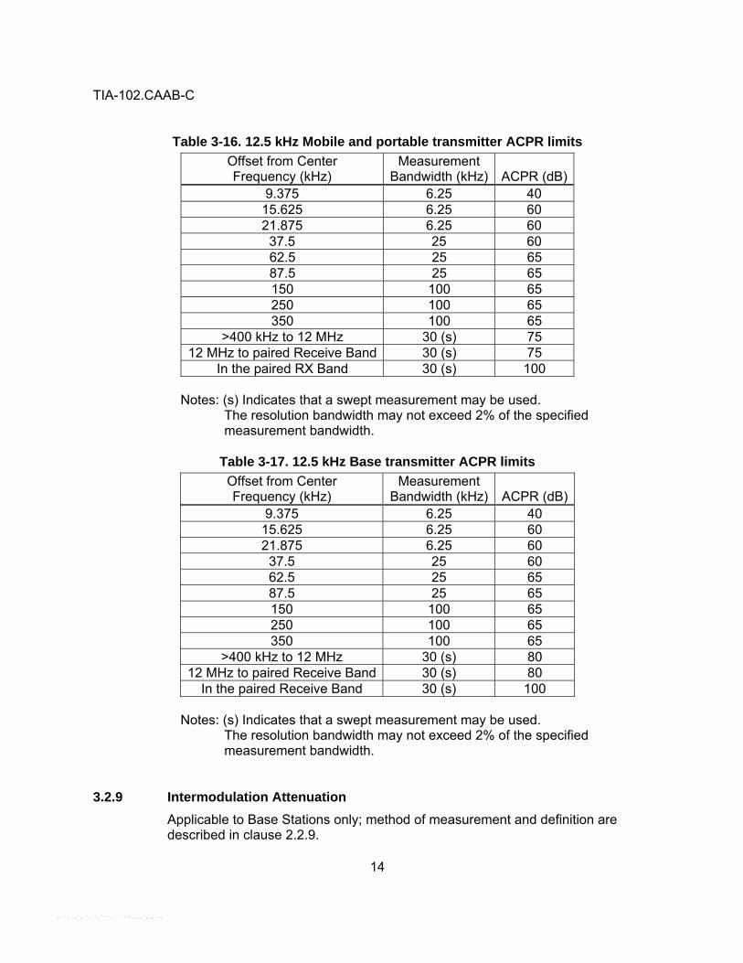
TIA-102.CAAB-C

14

Table 3-16. 12.5 kHz Mobile and portable transmitter ACPR limits

Offset from Center Frequency (kHz)

Measurement Bandwidth (kHz)

ACPR (dB)

9.375 6.25 40 15.625 6.25 60 21.875 6.25 60

37.5 25 60 62.5 25 65 87.5 25 65 150 100 65 250 100 65 350 100 65

>400 kHz to 12 MHz 30 (s) 75 12 MHz to paired Receive Band 30 (s) 75

In the paired RX Band 30 (s) 100

Notes: (s) Indicates that a swept measurement may be used. The resolution bandwidth may not exceed 2% of the specified

measurement bandwidth.

Table 3-17. 12.5 kHz Base transmitter ACPR limits Offset from Center Frequency (kHz)

Measurement Bandwidth (kHz)

ACPR (dB)

9.375 6.25 40 15.625 6.25 60 21.875 6.25 60

37.5 25 60 62.5 25 65 87.5 25 65 150 100 65 250 100 65 350 100 65

>400 kHz to 12 MHz 30 (s) 80 12 MHz to paired Receive Band 30 (s) 80

In the paired Receive Band 30 (s) 100

Notes: (s) Indicates that a swept measurement may be used. The resolution bandwidth may not exceed 2% of the specified

measurement bandwidth.

3.2.9 Intermodulation Attenuation Applicable to Base Stations only; method of measurement and definition are described in clause 2.2.9.

--```,``,,`,,``,```,`````,`````-`-`,,`,,`,`,,`---

TIA-102.CAAB-C

15

Standard The intermodulation attenuation shall meet or exceed 40 dB.

3.2.10 Radiated Power Output The method of measurement and definition are described in clause 2.2.10. The equipment position is to be specified by the manufacturer. The antenna position, mounting and type shall be specified by the manufacturer, and if applicable, shall be that normally supplied. The radiated output power shall be measured at Standard Test Voltage (Power Supply Voltage Range clause 3.3.1). Standard The Radiated Output Power shall conform to one or both of the clauses. Applicable to portable radios only.

3.2.10.1 Applicable to all frequency bands below 1 GHz excluding frequencies in the 700 MHz band as specified in 47 CFR 27.50 or 47 CFR 90.541.

The average radiated power output measured at Standard Test Voltage (Power Supply Voltage Range clause 3.3.1) shall meet or exceed the manufacturer's rating of average radiated power, and shall not exceed by more than 20% the rating for which the equipment has been type accepted by the FCC. No recommendations as to standardized Average Radiated Output Power levels are made.

3.2.10.2 Applicable to 700 MHz band

Equipment designed to operate in the 700 MHz band shall not exceed the limits in Table 3-18 per FCC 27.50 (b) (9) or (b) (10) or Table 3-19 per 90.541

Table 3-18. Part 27 Radiated power output limits Station Type Maximum ERP

Mobile 30 Watts Portable 3 Watts

Table 3-19. Part 90 Radiated power output limits Station Type Maximum ERP

Mobile 30 Watts Portable 3 Watts

Low Power Portable1 2 Watts Note 1: Narrowband lower power channels are listed in 90.531 (b) (3) and (b) (4).

--```,``,,`,,``,```,`````,`````-`-`,,`,,`,`,,`---

TIA-102.CAAB-C

16

3.2.11 Conducted Spurious Emissions into VSWR Applicable method of measurement and definition are described in clause 2.2.11. Standard (47 CFR 90.210(d)) Conducted spurious emissions shall be attenuated at least 50 + 10log(P) dB, or 70 dB, whichever is the lesser attenuation, when measured with any VSWR ≤ 3:1 for a mobile, ≤ 6:1 for a portable, and ≤ 2:1 for a base station.

3.2.12 Transmitter Power and Encoder Attack Time Applicable method of measurement and definition are described in clause 2.2.12 Standard for voice and circuit switched data service in a conventional non-trunked system. The transmitter power attack time shall not exceed 50 milliseconds. The transmitter encoder attack time shall not exceed 100 milliseconds

3.2.13 Transmitter Power and Encoder Attack Time with Busy/Idle Operation Applicable method of measurement and definition are described in clause 2.2.13 Standard for voice and circuit switched data service in a conventional non-trunked system The transmitter power attack time with busy/idle operation shall not exceed 30 milliseconds. The transmitter encoder attack time with busy/idle operation shall not exceed 30 milliseconds

3.2.14 Transmitter Throughput Delay Methods of measurement and definition are described in clause 2.2.14. Standard The transmitter throughput delay time for voice service shall not exceed 125 milliseconds.

3.2.15 Frequency Deviation for C4FM Applicable to C4FM transmitters only: methods of measurement and definition are described in clause 2.2.15. Standard High Level signal deviation shall exceed 2544 Hz but not exceed 3111 Hz. Low Level signal deviation shall exceed 848 Hz but not exceed 1037 Hz.

--```,``,,`,,``,```,`````,`````-`-`,,`,,`,`,,`---

TIA-102.CAAB-C

17

3.2.16 Modulation Fidelity

Methods of measurement and definition are described in clause 2.2.16. Standard For CQPSK or C4FM or standard simulcast modulation, when measured per the method of clause 2.2.16.2 the rms Error Magnitude shall not exceed the appropriate limit in Table 3-20.

Table 3-20. Modulation fidelity limits Radio Application Mobile Portable Base Station

Class A 5 % 5 % 5 % Class B 10 % 10 % 10 %

For CQPSK or C4FM or standard simulcast modulation, when measured per the method of clause 2.2.16.2 the carrier frequency offset shall not exceed the appropriate operating frequency error limit in the table of clause 3.2.2.2. For CQPSK or C4FM or standard simulcast modulation, when measured per the method of clause 2.2.16.2, the deviation shall exceed 1620 Hz but shall not exceed 1980 Hz. For C4FM only, when measured per the method of clause 2.2.16.4 the rms Error Magnitude shall not exceed the appropriate limit in Table 3-21.

Table 3-21. C4FM rms error magnitude limits Radio Application Mobile Portable Base Station

Class A 5 % 5 % 5 % Class B 10 % 10 % 10 %

For C4FM, when measured per the method of clause 2.2.16.4, the deviation shall exceed 1620 Hz but shall not exceed 1980 Hz. For C4FM only, when measured per the method of clause 2.2.16.4 the peak spurious frequency component amplitude shall not exceed the appropriate limit in Table 3-22.

Table 3-22. C4FM Peak spurious frequency limits Radio Application Mobile Portable Base Station

Class A 100 Hz 100 Hz 50 Hz Class B 150 Hz 150 Hz 100 Hz

3.2.17 Symbol Rate Accuracy

Applicable method of measurement and definition are described in clause 2.2.17.

--```,``,,`,,``,```,`````,`````-`-`,,`,,`,`,,`---

TIA-102.CAAB-C

18

Standard The symbol rate error shall not exceed 10 PPM.

3.2.18 Transient Frequency Behavior Applicable method of measurement and definition are described in clause 2.2.18. The standard that follows per Figure 1 and Figure 2 and Table 3-23 and applies to the mean frequency, which excludes peaks due to modulation. Standard (47 CFR 90.214)

-12.5

-6.25

0

6.25

12.5

t

Freq

uenc

y (k

Hz)

Per Clauses 3.2.2 plus 3.2.15

t1

t2

Figure 1 – Turn-on transient behavior and mean frequency limits

--```,``,,`,,``,```,`````,`````-`-`,,`,,`,`,,`---

TIA-102.CAAB-C

19

-12.5

-6.25

0

6.25

12.5

-2.5 2.5 7.5 12.5 17.5

t

Freq

uenc

y (k

Hz)

t3

Figure 2 – Turn-off transient behavior and mean frequency limits

Table 3-23. Mean transient frequency limits

Frequency Ranges (MHz)

Time Intervals 30 to 300 300 to 512 512 to 1000 t1 5.0 ms 10.0 ms 20.0 ms t2 20.0 ms 25.0 ms 50.0 ms t3 5.0 ms 10.0 ms 10.0 ms

During the period t1 and t3 the mean frequency difference shall not exceed ±12.5 kHz. During the period t2 the mean frequency difference shall not exceed ±6.25 kHz. If the transmitter carrier output power rating is 6 watts or less, the mean frequency difference during t1 and t3 may be greater than ±12.5 kHz. The corresponding plot of frequency versus time during t1 and t3 shall be recorded in the test data.

3.2.19 RFSS Throughput Delay Applicable method of measurement and definition are described in clause 2.2.19. Standard

--```,``,,`,,``,```,`````,`````-`-`,,`,,`,`,,`---

TIA-102.CAAB-C

20

The RFSS throughput delay shall not exceed 100 ms for simple repeaters. For other configurations of the RFSS the manufacturer shall specify the RFSS configuration and the average value that will not be exceeded.

3.2.20 RFSS Idle to Busy Transition Time Applicable method of measurement and definition are described in clause 2.2.20. Standard The RFSS idle to busy transition time shall not exceed 30 ms. For simulcast RFSS configurations the manufacturer shall specify the average value that will not be exceeded.

--```,``,,`,,``,```,`````,`````-`-`,,`,,`,`,,`---

TIA-102.CAAB-C

21

3.3 Trunked System Timing Characteristics

This clause defines performance limits for units intended for trunked system operation.

3.3.1 Trunking Control Channel Slot Times Applicable methods of measurement and definition are described in clause 2.3.1. Standard The trunking control channel encode attack time, trunking control channel RF power attack time, and trunking control channel RF power turn off time shall meet the control channel time slot duration dependent limits in Table 3-24.

Table 3-24. Trunking control channel slot time limits 37.5 ms slot 45 ms slot

Encode Attack Time 4.15 ms max. 2.00 ms min.

11.65 ms max. 2.00 ms min.

RF Power Attack Time 4.15 ms max. 0.00 ms min.

11.65 ms max. 0.00 ms min.

RF Power Turn Off Time 1.57 ms max. 1.57 ms max.

3.3.2 Trunking Request Time Applicable methods of measurement and definition are described in clause 2.3.2. Standard The trunking request time shall not exceed the slot time dependent limit in Table 3-25.

Table 3-25. Trunking request time limits 37.5 ms slot 45 ms slot

160 ms 167.5 ms

3.3.3 Trunking Voice Channel Access Time Applicable methods of measurement and definition are described in clause 2.3.3. Standard The trunking voice channel access time shall not exceed the limit specified by the manufacturer.

--```,``,,`,,``,```,`````,`````-`-`,,`,,`,`,,`---

TIA-102.CAAB-C

22

3.3.4 Time to Grant Applicable methods of measurement and definition are described in clause 2.3.4. Standard for non-simulcast systems The time to grant depends on the outbound signaling packet (OSP) duration and shall not exceed the inbound signaling packet (ISP) slot time dependent limits in Table 3-26.

Table 3-26. Non-Simulcast time to grant limits OSP duration 37.5 ms ISP 45 ms ISP

Single TSBK (37.5 ms) 337.5 ms 345.0 ms Double TSBK (60 ms) 354.0 ms 361.5 ms Triple TSBK (75 ms) 366.5 ms 374.0 ms

Standard for simulcast systems The time to grant depends on the outbound signaling packet (OSP) duration and shall not exceed the inbound signaling packet (ISP) slot time dependent limits in Table 3-27

Table 3-27. Simulcast time to grant limits OSP duration 37.5 ms ISP 45 ms ISP

Single TSBK (37.5 ms) 487.5 ms 495.0 ms Double TSBK (60 ms) 504.0 ms 511.5 ms Triple TSBK (75 ms) 516.5 ms 524.0 ms

3.3.5 Transmitter Time to Key on a Traffic Channel

Applicable methods of measurement and definition are described in clause 2.3.5. Standard for non-simulcast systems The RF transmitter time to key on a working channel and encoder transmit time depend on the working channel form and shall not exceed the limits in Table 3-28.

Table 3-28. Transmitter time to key on a traffic channel limits Short channel form Explicit channel form

RF transmitter time to key on a working channel 150.0 ms 171.1 ms

Encoder transmit time 150.0 ms 171.1 ms

--```,``,,`,,``,```,`````,`````-`-`,,`,,`,`,,`---

TIA-102.CAAB-C

23

3.4 Unit Characteristics This clause defines allowed degradation from standards (DFS) in clauses 3.1 and 3.2, in accordance with clause 1.3.5 for performance under specific environmental parameter conditions. No DFS, where used, means no degradation from the standard is allowed. Unless otherwise specified, all tests shall be done at the standard atmospheric conditions specified in clause 1.4.5. All equipment shall meet all standards in clauses 3.4.1 through 3.4.9. Class A equipment shall also meet all standards in clause 3.4.10.1 through 3.4.10.5. All equipment to be installed in marine or airborne environments shall meet the appropriate vibration standard in clause 3.4.10.6 through 3.4.10.8.

3.4.1 Power Supply Voltage Range Applicable methods of measurement and definition are described in clause 2.4.1. For tests on a portable the battery may be disconnected but not removed, per clause 1.4.4.1. Standard The equipment shall meet the allowable performance degradations specified for each test listed in the succeeding summary table when tested at the Standard Test Voltage specified in clause 1.4.4, as well as at the voltage variation limits specified in the summary table. Normally these tests are conducted with the battery not connected. Should tests be conducted with the battery connected, under no circumstances are test voltages to exceed the safe operating range of the battery technology specified by the manufacturer of the equipment. The limit voltages shall be at least either ±10% or ±20% voltage range from the standard test voltage as required by the specific test, or; a) Receivers only;

At the highest and lowest receiver voltages encountered during the portable equipment Battery Life (per clause 3.4.7).

b) Transmitters only; At the highest and lowest transmitter voltages encountered during the portable equipment Battery Life (per clause 3.4.7).

Table 3-29 summarizes the tests to be performed, the limit voltage conditions, and degradation allowances for both class A and Class B:

--```,``,,`,,``,```,`````,`````-`-`,,`,,`,`,,`---

TIA-102.CAAB-C

24

Table 3-29. Power supply variation tests and DFS limits

Standard

Specification Limit @ ±10% except where stated otherwise

3.1.4 Reference sensitivity 3 dB DFS @ ±20% 3.1.7 Adjacent Channel Rejection 2 dB DFS

3.1.8 Co-Channel Rejection 2 dB DFS 3.1.9 Spurious Response Rejection no DFS

3.1.10 Intermodulation Rejection 3 dB DFS 3.1.11 Signal Displacement BW no DFS 3.1.12 Audio Output Distortion

(Base Station only) (Mobile and Portable only)

(All radios)

<5% @ the following levels: Full rated power

Rated power less 3dB Rated power less 17dB

3.1.16 Bit Error Rate Floor 0.1 % 3.2.1 RF Output Power

(Base Station only) (Mobile and Portable only)

(All radios)

3 dB DFS @ ±20% 6 dB DFS @ ±20% 3 dB DFS @ ±10%

3.2.2 Operating Frequency Accuracy no DFS @ ±20% 3.2.3 Electrical Audio Performance 1 dB DFS 3.2.9 Intermodulation Attenuation 5 dB DFS

3.2.11 Conducted Spurious Emissions into VSWR No DFS

3.2.16 and/or 3.2.15 Transmitter Fidelity No DFS

3.2.16 Symbol Rate Accuracy No DFS -

-```,``,,`,,``,```,`````,`````-`-`,,`,,`,`,,`---

TIA-102.CAAB-C

25

3.4.2 Temperature Range Applicable method of measurement and definition are described in clause 2.4.2. Standard a) The lower temperature limit for all equipment is -30 °C. b) The upper temperature limit for all equipment is +60 °C. The tests listed in Table 3-30 should be performed for all equipment and results observed at both the lower and upper temperature limits using standard voltage, and ±10% voltage limits except where otherwise specified.

Table 3-30. Extreme Temperature tests and DFS limits Standard

Limit for Standard Voltage

Per 1.4.4

Limit for ±10% Limit Voltages

Per 3.4.1 3.1.4 Reference sensitivity 6 dB DFS 8 dB DFS 3.1.7 Adjacent Channel Rejection (Base Station only) (Mobile and Portable)

4 dB DFS

13 dB DFS

4 dB DFS

13 dB DFS 3.1.8 Co-Channel Rejection 2 dB DFS 3 dB DFS 3.1.9 Spurious Response Rejection (Base Station only) (Mobile and Portable)

6 dB DFS

10 dB DFS

6 dB DFS

10 dB DFS 3.1.10 Intermodulation Rejection (Base Station only) (Mobile and Portable)

6 dB DFS 6 dB DFS

6 dB DFS

10 dB DFS 3.1.11 Signal Displacement BW 500 Hz DFS 500 Hz DFS 3.1.12 Audio Output Distortion (Base Station only) (Mobile and Portable only) (All radios)

<5% @ rated power less: 0 dB 3 dB

17 dB


17 dB 3.1.16 Bit Error Rate Floor 0.5 % 0.5 % 3.2.1 RF Output Power 3 dB DFS 6 dB DFS 3.2.2 Operating Freq. Accuracy no DFS No DFS @ ±20% 3.2.3 Electrical Audio Performance 1 dB DFS 2 dB DFS 3.2.9 Intermodulation Attenuation 5 dB DFS 11 dB DFS 3.2.11 Conducted Spurious Emissions into VSWR No DFS No DFS

3.2.16 and/or 3.2.15 Transmitter Fidelity No DFS No DFS

3.2.16 Symbol Rate Accuracy No DFS No DFS

--```,``,,`,,``,```,`````,`````-`-`,,`,,`,`,,`---

TIA-102.CAAB-C

26

3.4.3 High Humidity Applicable method of measurement and definition are described in clause 2.4.3. Standard a) The relative humidity shall be between 90% and 95% at a temperature of

+50°C. b) The tests listed in Table 3-31 shall be performed on all equipment and results

observed while the equipment is subjected to the specified relative humidity at standard voltage, and at ±10% limit voltages except where specified otherwise:

Table 3-31. Relative humidity tests and DFS limits

Standard

Limit for Standard Voltage Per 1.4.4

Limit for ±10% Limit Voltages Per 3.4.1

3.1.4 Reference sensitivity 6 dB DFS 8 dB DFS 3.1.7 Adjacent Channel Rejection (Base Station only) (Mobile and Portable)

4 dB DFS 13 dB DFS

4 dB DFS 13 dB DFS

3.1.7 Co-Channel Rejection 2 dB DFS 3 dB DFS 3.1.9 Spurious Response Rejection (Base Station only) (Mobile and Portable)

6 dB DFS 10 dB DFS

6 dB DFS 10 dB DFS

3.1.10 Intermodulation Rejection (Base Station only) (Mobile and Portable)

6 dB DFS 6 dB DFS

6 dB DFS 10 dB DFS

3.1.11 Signal Displacement BW 500 Hz DFS 500 Hz DFS 3.1.12 Audio Output Distortion

(Base Station only)

(Mobile and Portable only) (All radios)


17 dB

<5% @ rated power less:

0 dB 3 dB

17 dB 3.1.16 Bit Error Rate Floor 0.5 % 0.5 %

3.2.1 RF Output Power 3 dB DFS 6 dB DFS 3.2.2

Operating Frequency Accuracy no DFS no DFS @ ±20%

3.2.3 Electrical Audio Performance 1 dB DFS 2 dB DFS 3.2.9 Intermodulation Attenuation 5 dB DFS 10 dB DFS

3.2.11 Conducted Spurious Emissions into VSWR No DFS No DFS

3.2.16 and/or 3.2.15 Transmitter Fidelity No DFS No DFS

3.2.17 Symbol Rate Accuracy No DFS No DFS

--```,``,,`,,``,```,`````,`````-`-`,,`,,`,`,,`---

TIA-102.CAAB-C

27

3.4.4 Vibration Stability Applicable method of measurement and definition are described in clause 2.4.4. Standard No fixed part shall become loose or any moveable part shift in position or adjustment under either of the two conditions of vibration. The vibration test shall consist of two parts: a) A mobile or portable unit shall complete three 5 minute cycles of simple

harmonic motion having an amplitude of 0.38 mm (total excursion of 0.76 mm) applied initially at a frequency of 10 Hz and increased at a uniform rate to 30 Hz in 2.5 minutes, then decreased at a uniform rate to 10 Hz in 2.5 minutes. The amplitude shall be 0.07 mm for a base station unit.

b) The unit shall next complete three 5 minute cycles of simple harmonic motion

having an amplitude of 0.19 mm (total excursion 0.38 mm) applied initially at a frequency of 30 Hz and increased at a uniform rate to 60 Hz in 2.5 minutes, then decreased at a uniform rate to 30 Hz in 2.5 minutes. The amplitude shall be 0.035 mm for a base station unit.

The above two-part test shall be applied for a total of 30 minutes in each of three directions, namely the directions parallel to both axes of the base and perpendicular to the plane of the base. The following tests shall be performed and the results observed shall be within the limits specified in Table 3-32.

Table 3-32. Vibration stability tests and DFS limits Standard Degradation Allowed

3.1.4 Reference Sensitivity No DFS 3.2.1 RF Output Power No DFS

3.2.2 Operating Frequency Accuracy No DFS

3.4.5 Shock Stability Applicable to Mobiles and Portables only; method of measurement and definition in

clause 2.4.5. Mobile Standard Mobile equipment shall meet all the requirements of clauses 3.1 and 3.2 and suffer no more than superficial mechanical damage after being subjected to a series of not less than ten impacts in each plane (total thirty). Each impact shall consist of a half sine wave acceleration pulse of 20g peak amplitude and 11 milliseconds duration.

--```,``,,`,,``,```,`````,`````-`-`,,`,,`,`,,`---

TIA-102.CAAB-C

28

Acceleration shall be applied to the manufacturer's mounting facilities and may be measured by means of a suitable accelerometer. The equipment shall be operated under standard test conditions and during half the impacts in each plane. Portable Standard Portable equipment shall suffer no more than superficial mechanical damage and shall meet all the standards of clauses 3.1 and 3.2 without degradation after being shocked. Shock will be delivered to the equipment by a drop test onto a smooth concrete floor with non-restrictive guides to assure free-fall dropping on the equipment surface being tested. Portable equipment shall be dropped once on each of six surfaces from a height of 100 cm. Onto a smooth concrete floor.

3.4.6 DC Supply Noise Susceptibility Applicable method of measurement and definition in clause 2.4.6. Standard The equipment shall be capable of no more than a 6 dB degradation in the residual audio noise ratio specification of clauses 3.1.12 when ripple with the following noise voltage characteristics are applied per Table 3-33.

Table 3-33. DC supply noise susceptibility characteristics Equipment type Frequency Range(Hz) Amplitude (mV peak to peak)

Base Station 50 to 40,000 100

Mobile and Portable 400 to 8,000

500 (or 100, only if the equipment is to be directly

connected to vehicular battery)

3.4.7 Battery Life

Applicable to Portables only; method of measurement and definitions are described in clauses 1.3.2.3 and 2.4.7. Standard for equipment consisting of a transmitter and a receiver The radio battery shall power the equipment for at least 8 hours when operated at the standard duty cycle. For equipment with a manufacturer specified battery life of less than 16 hours, the standard duty cycle shall be performed over the hours specified by the manufacturer.

--```,``,,`,,``,```,`````,`````-`-`,,`,,`,`,,`---

TIA-102.CAAB-C

29

For equipment with a manufacturer specified battery life in excess of 16 hours, the standard duty cycle shall be performed for 8 hours followed by 16 hours rest. Standard for equipment consisting only of a voice receiver The radio battery shall power the equipment for at least 8 hours when operated at a duty cycle comprised of 6 seconds receive at manufacturer's stated audio output power and 54 seconds standby. Standard for equipment consisting only of a transmitter The radio battery shall power the equipment for at least 8 hours when operated at a duty cycle of 6 seconds transmit at manufacturer's stated RF output power and 54 seconds standby.

3.4.8 Dimensions Applicable method of measurement and definition are described in clause 2.4.8. The manufacturer shall specify the dimensions per clause 2.4.8.2. Portable equipment shall be measured together with all accessories required for operation and support during its intended use with the exception that an antenna that protrudes beyond the basic equipment case may be excluded from the size measurement. Standard The size of the equipment, in metric units, shall not exceed the manufacturer's specifications.

3.4.9 Weight Applicable method of measurement and definition are described in clause 2.4.9. The manufacturer shall specify the weight per clause 2.4.9.2. Portable equipment shall be weighed together with all accessories required for operation and support during its intended use. Standard The weight of the equipment, in metric units, shall not exceed the manufacturer's specifications.

3.4.10 Other Environmental Applicable to Class A mobile and portable equipment only. The assessment methods to be used are described in MIL-STD-810E for the methods, procedures and categories listed in subsequent clauses 3.3.10.1 through 3.3.10.8, and MIL-STD-167 for clause 3.3.10.8. Specific test conditions and

--```,``,,`,,``,```,`````,`````-`-`,,`,,`,`,,`---

TIA-102.CAAB-C

30

tailoring are specified herein utilizing Tables and Figures contained in the applicable MIL-STD document.

3.4.10.1 Rain

3.4.10.1.1 Applicable Method 506.3, Procedure I - Blowing Rain

3.4.10.1.2 Specific Test Conditions and Tailoring

The equipment shall be powered on for the entire duration of the test. Emulated rainfall shall be applied at a rate of 5.2 inches per hour. Standard The equipment shall meet the standards in clauses 3.1 and 3.2 herein with no DFS immediately after being exposed, and there shall be no evidence of water penetration.

3.4.10.2 Salt Fog

3.4.10.2.1 Applicable Method 509.3, Procedure I - Aggravated Screening


Equipment shall not be powered at any time during the continuous 48 hour exposure. Standard The equipment shall meet the standards in clauses 3.1 and 3.2 herein with no DFS when operated at the end of the 48 hour drying period. No potential future effects on proper functioning of the equipment shall be evident from an analysis of corrosion, electrical, and physical effects resulting from the test environment.

3.4.10.3 Sand and Dust

3.4.10.3.1 Applicable Method 510.3, Procedure I - Blowing Dust, and Procedure II - Blowing Sand


The equipment shall not be powered at any time during the duration of the exposure. Sand shall be blown at a speed of 3540 to 5700 feet per minute for 90 minutes on each surface. Dust shall be blown at a speed between 300 and 1750 feet per minute for 6 hours at 23 °C, then 6 hours at 71 °C. Standard The equipment shall meet the standards in clauses 3.1 and 3.2 herein with no DFS when operated after removal from test environment, and after removal of accumulated dust by brushing, wiping, or shaking. Dust shall not be removed by either air blast or vacuum cleaning. No potential future effects on proper operation of the equipment shall be evident from an analysis of effects resulting from the test environment.

TIA-102.CAAB-C

31

3.4.10.4 Shock

3.4.10.4.1 Applicable Method 516.4, Procedure I - Functional Shock


The equipment shall not be powered at any time for the duration of the exposure. The shock response spectrum shall be per Figure 516.4-1 functional test for ground equipment (40 g peak acceleration). Test axes and number of shocks shall be 3 times in both directions along each of three orthogonal axes (total of 18 shocks). Standard After being shocked the equipment shall meet all standards in clauses 3.1 and 3.2 herein with no DFS; shall suffer no physical damage; and no fixed part shall become loose or any moveable part shift in position or adjustment.

3.4.10.5 Vibration (Ground Mobile)

3.4.10.5.1 Applicable Method 514.4, Procedure I, Category 8 for mobile equipment, and portable equipment with vehicle mounted adapter, to be mounted in a terrestrial vehicle.


The equipment shall not be powered at any time during the test. Random vibration shall be applied per Figure 514.4-16. Test duration and axes shall be per Table 514.4-VII for 1 hour per axis along 3 orthogonal axes. Sinusoidal vibration shall be applied per Figure 514.4-17. Test duration and axes shall be per Table 514.4-VII for 3 hours per axis along 3 orthogonal axes using a 30 minute logarithmic sweep from 5 Hz to 500 Hz. Standard After sinusoidal and random vibration exposure the equipment shall meet all standards in clauses 3.1 and 3.2 herein with no DFS; shall suffer no physical damage; and no fixed part shall become loose, or any moveable part shift in position or adjustment.

3.4.10.6 Vibration (Helicopter)

3.4.10.6.1 Applicable Method 514.4, Procedure I, Category 6 only for mobile equipment, and portable equipment with vehicle mounted adapter, to be mounted in a helicopter.


The equipment shall not be powered at any time during the test. Sinusoidal vibration shall be applied per Figure 514.4-17. Test duration and axes shall be per Table 514.4-VII for 3 hours per axis along 3 orthogonal axes using a 30 minute logarithmic sweep from 5 Hz to 500 Hz.

--```,``,,`,,``,```,`````,`````-`-`,,`,,`,`,,`---

TIA-102.CAAB-C

32

Random vibration shall be applied per Figure 514.4-9. Test duration and axes shall be per Table 514.4-IV for 1 hour per axis along 3 orthogonal axes. Standard After sinusoidal and random vibration exposure the equipment shall meet all standards in clauses 3.1 and 3.2 herein with no DFS; shall suffer no physical damage; and no fixed part shall become loose, or any moveable part shift in position or adjustment.

3.4.10.7 Vibration (Propeller Aircraft)

3.4.10.7.1 Applicable Method 514.4, Procedure I, Category 4 only for mobile equipment, and portable equipment with vehicle mounted adapter, to be mounted in a propeller driven aircraft.


The equipment shall not be powered at any time during the test. Random vibration shall be applied per Figure 514.4-7. Test duration and axes shall be per Table 514.4-II for 1 hour per axis along 3 orthogonal axes. Standard After vibration the equipment shall meet all standards in clauses 3.1 and 3.2 herein with no DFS; shall suffer no physical damage; and no fixed part shall become loose, or any moveable part shift in position or adjustment.

3.4.10.8 Vibration (Marine)

3.4.10.8.1 Applicable Method 514.4, Procedure I, Category 9 only for mobile equipment, and portable equipment with vehicle mounted adapter, to be mounted in a marine vessel.


The equipment shall not be powered at any time during the test. Sinusoidal vibration shall be applied per MIL-STD-167 type I - Environmental. Test duration and axes shall be 3 hours per axis along 3 orthogonal axes using a 30 minute logarithmic sweep from 5 Hz to 500 Hz. Random vibration shall be applied per Figure 514.4-15. Test duration and axes shall be for 2 hours per axis along 3 orthogonal axes. Standard After sinusoidal and random vibration exposure the equipment shall meet all standards in clauses 3.1 and 3.2 herein with no DFS; shall suffer no physical damage; and no fixed part shall become loose or any moveable part shift in position or adjustment.

TIA-102.CAAB-C

33

ANNEX A Measurement Uncertainty (Informative)

A.1 Introduction Since two observers making measurements on the same Unit Under Test will not obtain the same results, it is important that the measurement uncertainties be understood by both observers and a consistent method of determining these uncertainties be used. This appendix will not attempt to make a statement about the confidence level of the measurement uncertainties, but it will provide a consistent method that will allow two observers to compare their results. It also provides a method for evaluating and calculating the uncertainties when performing measurements to the limits specified in sections 3.1 through 3.4. This Annex contains: a) A tutorial on the types of measurement errors that can occur and provides a mathematical method to quantify these errors. b) Example calculations for the measurement methods in sections 2.1, 2.2 and 2.3. These examples may be used without an understanding of the mathematical derivations in section 3. The sources of errors listed in the example calculations may not include all the possibilities. Therefore, it is important that the observers identify all of the errors for their measurements and perform the analysis.

A.2 Definitions

A.2.1 Accuracy The degree of closeness of a stated value to the actual or true value. While a commonly-used term, its definition is not precise. Therefore, the term "uncertainty" will be used in preference to "accuracy" in this document.

A.2.2 Measurand A quantity subject to measurement.

A.2.3 Error The difference between the measured value and the true value of a measurand.

A.2.4 Bias and Systematic Error The difference between the expectation of the measured value and the true value of the measurand. The bias error is constant for a set of measurements performed on the same device, using the same measurement setup, performed within a reasonably short time frame. Bias error is the same as systematic error.

--```,``,,`,,``,```,`````,`````-`-`,,`,,`,`,,`---

TIA-102.CAAB-C

34

A.2.5 Random Error The difference between the measured value and the limiting mean, or expectation, of those values; the difference between the measured value and the bias error. The random error is different each time a measurement is performed.

A.2.6 RSS Errors Errors that are combined by calculating the square root of the sum of the square of the individual errors.

A.2.7 Precision A measure of the reproducibility of the measurement results made under one set of conditions; a measure of the spread of random error. Precision is often expressed in terms of the standard deviation of the measurements, or in terms of a confidence limit. The standard deviation may be determined each time the measurement is performed, or just once, using a very large set of measurements, to arrive at a more reliable estimate as long as it doesn't change among measurement sets, e., as long as the measurement process is stationary. In some cases where the distribution of measured values about its mean is known theoretically from the nature of the measurement, the standard deviation may be determined a prior

A.2.8 Uncertainty An estimate characterizing the range of values within which the true value of a measurand lies.

A.2.9 Confidence Limits Those values which the random component of error has some stated probability of being within; the random component of uncertainty.

A.3 Principles for Calculating Measurement Uncertainties A.3.1 General

When calculating the over all measurement uncertainty for a given method of measurement, one has to identify all of the individual errors and sum these errors. There are several different methods discussed on the ways to sum the errors. This appendix will use a method sufficient for transceiver test while providing a reasonable calculation.

A.3.2 Types of Errors A.3.2.1 Random Errors

From Murphy [1969, p. 360] Sometimes the precision is stated as ±2 standard deviations with the implication that approximately 95% of all the measurements of the measurement process will fall within two standard deviations of the long-run average for that process, whether

--```,``,,`,,``,```,`````,`````-`-`,,`,,`,`,,`---

TIA-102.CAAB-C

35

that long-run average agrees with the reference level [e., true value] or not. In some cases people have used the multiple 1.96 rather than 2 in the hope that they will have obtained limits which more truly represent actual bounds within which 95% of the universe will lie. Usually such refinements are specious on two grounds: first, because the accuracy with which the standard deviation will be known is not consistent with distinguishing between multipliers of 2.00 and 1.96; second, too great a reliance on the figure of 95% is unjustifiable, anyway, since some measurement processes will yield a universe of observations of which perhaps only 90% may lie within the 2-standard-deviation limits. It is reasonable to suppose in most cases, however, that such limits will include 90% to 95% of the statistical universe of observations. Because of the uncertainty associated with this multiple, it might usually be better avoided in favor of other alternatives.

A.3.2.2 Bias Errors

The overall systematic or bias error of a measurement is generally composed of a number of individual systematic errors. From Eisenhart [1969, p. 43]: Since the "known" systematic errors affecting a measurement process ascribable to specific origins are ordinarily determinate in origin only, their individual values ordinarily being unknown both with respect to sign and magnitude, it is not possible to evaluate their algebraic sum and thereby arrive at a value for the overall systematic error of the measurement process concerned. In consequence, it is necessary to arrive at bounds for each of the individual components of systematic error that may be expected to yield non-negligible contributions, and then from these bounds arrive at credible bounds to their combined effect on the measurement process concerned. Both of these steps are fraught with difficulties. Determination of reasonable bounds to the systematic error likely to be contributed by a particular origin or assignable cause necessarily involves an element of judgment, and the limits cannot be set in exactitude. By assigning ridiculously wide limits, one could be practically certain that the actual error due to a particular cause would never lie outside of these limits. But such limits are not likely to be very helpful. The narrower the range between the assigned limits, the greater the uneasiness one feels that the assigned limits will not include whatever systematic error is contributed by the cause in question. But a decision has to be made; and on the basis of theory, other related measurements, a careful study of the situation in hand, especially its sensitivity so small changes in the factor concerned, and so forth, "the experimenter presently will feel justified in saying that he feels, or believes, or is of the opinion," that the systematic error due to the particular source in question does not exceed such and such limits, "meaning thereby, since he makes no claim to omniscience, that he has found no reason believing" that it exceeds these limits. In other words, "nothing has come to light in the course of the work to indicate" that the systematic error concerned lies outside the stated range.

--```,``,,`,,``,```,`````,`````-`-`,,`,,`,`,,`---

TIA-102.CAAB-C

36

Given the above statement, the problem remains how to combine individual sources of systematic error into one estimate of bias. The commonly used methods are: a) Take the sum of the individual limits. b) Take the square root of the sum of the squares of the individual limits that are

expressed in fraction form of (delta X)/(X). c) Assume a probability distribution for each of the individual systematic errors

and calculate the probability distribution of their sum, assuming that the sources of error are independent. The estimated limits of the total bias error is then taken to be the points on the probability distribution function of the sum that encompass some fraction, typically 95%, of all the possible values.

Method a) is simple and often suitable when the number of individual sources of error is small, say 3 or less. It is probably overly pessimistic, however, when the number of errors is larger, as it seems very unlikely that all of the errors would be of the same sign and of the largest expected magnitude. Method c) is initially attractive from a theoretical standpoint, though it can be computationally complex when the number of sources is not large and their limits are not of similar magnitude. Further, it suffers the problem that the underlying assumption of the applicability of the theory of error to the problem is not strictly valid. It assumes that the systematic errors actually do vary from one test setup to another according to the probability distribution function and that over a large number of such setups, some fraction of the systematic errors will lie within the limits given by that fraction of the distribution function. The assumption also implies that over a large number of such setups, the average systematic error will tend to zero. There is typically no evidence to support this assumption. There is no basis in statistical theory for assigning a confidence level to the bias error so determined. [Dorsey and Eisenhart 1969, p.50.] Consequently, this standard will adopt method b) as the means of combining independent systematic errors since it provides a more reasonable estimate of the bias error limits than a), is commonly accepted, is computationally simpler than c) and does not lead one as easily to draw unsupported conclusions as the latter. As a comparison between methods b) and c), it may be noted that the limits computed by b) encompass between 94 and 100% of the error distributions computed as in c), if the individual errors are assumed to be uniformly distributed between their limits. If limits are calculated per c) using a "confidence level" of 95%, the calculated limits are from 5% less to 13% greater than those calculated using b). The effect of some systematic errors can be minimized by applying a correction factor to the measurement results when the value of the error and its effect on the measurement results are known. If the value of the systematic error itself is the result of a measurement, the errors in that measurement must be appropriately applied to the final uncertainty. An example of this is correcting modulation deviation measurements for the effect of residual noise.

--```,``,,`,,``,```,`````,`````-`-`,,`,,`,`,,`---

TIA-102.CAAB-C

37

A.3.3 Propagation of Errors

A.3.3.1 General

If some quantity z is calculated as a function of two other quantities x and y, then for some nominal or reference values x0 and y0 ,

z0 = f(x0 , y0) (1)

and for small deviations from this nominal value,

z0 + dz = f(x0 + dx, y0 + dy). (2)

first-order approximation, good for dx and dy much smaller than x0 and y0, respectively,

0 0 0 x=xy=y

x=xy=y

z + dz = f ( x , y ) + fx

dx| + fy

dy|00

00

∂∂

∂∂

(3)

dz = fx

dx| + fy

dy| x= xy= y

x= xy= y

00

00

∂∂

∂∂

(4)

If dx and dy are taken to represent errors in x and y, respectively, then dz is the error in z that results from those errors.

A.3.3.2 Propagation of Random Errors If x and y are random variables, as for example measurements having random errors, then z is also a random variable, and to a first-order approximation,

µz = f(µx , µy ) (5)

σ σ σ ρ σ σ∂∂

∂∂

∂∂

∂∂z

fx x

fy y xy

fx

fy x y

2 2 2 22 2

= ⎡⎣⎢

⎤⎦⎥

⎡

⎣⎢

⎤

⎦⎥+ + (6)

for σx and σy sufficiently small that f(x, y) is nearly linear in the vicinity of μx and μy. The square brackets signify that the derivatives within the brackets are to be evaluated at μx and μy. If x and y are uncorrelated (usually true if they are independent), then the correlation coefficient ρxy is zero and the second equation reduces to

σ σ σ∂∂

∂∂z

fx x

fy y

2 2 22 2

= ⎡⎣⎢

⎤⎦⎥

⎡

⎣⎢

⎤

⎦⎥+ (7)

The extension to functions of more than two variables is straightforward.

--```,``,,`,,``,```,`````,`````-`-`,,`,,`,`,,`---

TIA-102.CAAB-C

38

A.3.4 Converting Power Errors Expressed in dB to Percentage

A bias error having [power] limits of ±ε% may be expressed in dB using the relations δ+ = 10 log10(1 + ε/100) (8)

δ- = 10 log10(1 - ε/100) (9)

However, for small ε, δ±(dB) ≅ (10/ln(10))×(±ε/100) = 0.04343×(±ε) (10)

The conversion formula of equation (10), and the equivalent for voltage bias errors, will be used in this document since it is sufficiently accurate for our purposes, avoids the problem of asymmetric error limits, and is consistent with other commonly used approximations. For example, error limits of ±0.22 dB may be converted to an equivalent power bias error of ±5.07% using our approximation, while the exact limits are +5.20, -4.94%. However, if a measurement result is calculated as the ratio of two measured values, each having error limits of ±5%, it is common to attribute ±5% of the error in the ratio to the error in the denominator, while the error in the denominator actually has a +5.26, -4.76% effect on the ratio. Hence the conclusion that our approximation is consistent with (and actually better than) others commonly used. Since symmetric percentage error limits yield asymmetric limits in dB, and vice versa, it is prudent to express the total measurement uncertainty in the same units as the largest error contributions.

A.3.5 Mismatch Uncertainty and Mismatch Loss When two instruments in a measurement configuration are connected, there will be a mismatch uncertainty of the signal passing through the connection. The mismatch uncertainty is described by the following equation:

Mu(dB) =10 log10(1 ± rg×rl)2 (11)

If the mismatch uncertainty limits are given in percent deviation from unity rather than in dB, then the equation becomes:

Mu(%)= 100 [x(1 ± rlxrg)2-1] (12)

Like equations (8) and (9), Mu is an asymmetric number; but, by applying equation (10) the following approximation can be used.

--```,``,,`,,``,```,`````,`````-`-`,,`,,`,`,,`---

TIA-102.CAAB-C

39

Mu(dB) ≅ 8.686xrgxrl (13)

where rl is the reflection coefficient of the load. rg is the reflection coefficient of the generator.

A.3.6 Sensitivity of Transmitter Output to Load A transmitter is usually designed to work into a 50 ohm load. If the load is not exactly 50 ohms, then there will be an uncertainty in any measurements requiring knowledge of the transmitter's output power. The following method of measurement will determine an effective output VSWR for the transmitter. For the examples in this appendix we will use an effective transmitter VSWR of 2:1.and a standard load input VSWR of 2:1. This gives an uncertainty value of 0.26 dB for the transmitter output to standard load.

a) Connect the equipment as illustrated in Figure A1.

DIRECTIONAL

TERMINATION

RF POWER

COUPLER

TERMINATION

UNDER TEST

50 OHM

TRANSMITTER

ANALYZERNETWORK

ATTENUATOR

175 MHzAbove

METERIMPEDANCE

STRETCHER

CONSTANT

VARIABLE

175 MHz

Below50 OHMLCLS

Figure A.1 – Test system block diagram

b) For frequencies up to 175 MHz, recommend using a lumped constant line stretcher (LCLS) as the variable load (see section 5.25, 5.26 for the typical values of the inductors and capacitors).

c) For frequencies above 175 MHz, use constant impedance line stretcher with a RF short as the variable load.

d) Select the value for the attenuator to produce a VSWR of 3:1. The equivalent reflection coefficient is then rl =0.5.

e) Calibrate the variable load using the network analyzer at the frequencies of interest.

f) Key the transmitter into the 50 ohm load and measure the level at the RF power meter. Record this level as Pz0 .

TIA-102.CAAB-C

40

g) Key the transmitter into the variable load. Vary the phase of the load to find the maximum level into the RF power meter. Record this value as Pfmax.

h) Repeat step g) but vary the phase of the load to find the minimum level into the RF power meter. Record this value as Pfmin.

I) The output reflection coefficient (rg) can be calculated from the maximum value of the following:

rg1 =

1− Pz0

Pf max

r1 (14)

rg2 =

1− Pz0

Pf max

r1 (15)

The maximum of rg1 and rg2 is rg

j) The effective output VSWR of the transmitter is now calculated as:

VSWR =1+ rg

1− rg (16)

A.3.7 Correcting rms Measurements for the Effects of rms Residuals Because sinusoidal signals and random noise are uncorrelated, their mean-squared voltages add. Therefore, the measured rms value of a signal in the presence of noise will be

T S2

N2V = V + V (17)

where Vs is the rms value of the signal and VN is the rms value of the noise. If the signal level does not influence the noise level (as it might if an AGC circuit was in the signal path), then a separate measurement of VN may be made and used to correct the measurement of VT to obtain a closer estimate of VS . The

estimate of VS ( )^Vs is then

S T

2

N

2

V = V - V^ ^ ^

(18)

Taking partial derivatives and applying the propagation of error formulas, we find that the normalized error in the measurement of VS is:

S

S

T2

T2

N2

T

T

N2

T2

N2

N

N

dVV

= VV -V

VV

- VV -V

VV

δ δ

(19) Example: Let the measurement of the rms deviation of an FM signal in the presence of noise be 2.20 kHz and the measurement of residual noise alone be 100 Hz. Further, let

--```,``,,`,,``,```,`````,`````-`-`,,`,,`,`,,`---

TIA-102.CAAB-C

41

the specified accuracy of the modulation meter be 2% of reading plus 10 Hz. Let us say that the measurements are stable so there is no need to include the effects of random errors. The normalized (systematic) error in the measurement of the total deviation is 2% + 100x10/2200 = 2.45%; that of the residual noise is 2% + 100x10/100 = 12%. Therefore, taking the root-sum-square of the two components, the normalized error in the determination of the signal deviation is:

(1.00× 2.45)2 + (0.00207 ×12)2 = 2.45% (20) In this example the contribution of the error in the measurement of residual noise is negligible. It also turns out that the residual noise itself has a negligible effect on the measurement of the signal level--it only corrects the measurement by 2.3 Hz, or 0.1%. This example shows that residual noise typically has a very small effect on rms measurements at typical signal-to-noise ratios.

A.3.8 Correcting Peak Measurements for the Effects of Residuals The response of a peak detector to noise and a signal plus noise depends, in a complicated fashion, on a number of factors beyond the control and knowledge of the typical user. It is not possible, therefore, to provide an accurate rule in the general case for correcting peak measurements for the effect of noise. The best that can be said is that it is very unlikely that a peak measurement of a signal made in the presence of noise will be less than that of the signal alone or greater than the sum of the signal and noise each measured alone.

--```,``,,`,,``,```,`````,`````-`-`,,`,,`,`,,`---

TIA-102.CAAB-C

42

ANNEX B Example Calculations (Informative)

B.1 Example Calculations for Receiver Measurements The examples in this section are for the limits in Section 3 based on the methods of measurement in Section 2.1 and the characteristics of equipment in Section 1.5 of ANSI/TIA/EIA 102.CAAA. Conversion between decibels and percentage used herein utilize the symmetric approximation described in equation 10 of Appendix A.

B.1.1 Radiated Spurious Emission Uncertainty sources and estimates:

Table B.1. 1Radiated spurious emission errors

Test site and antenna 3 dB 69%

Test cable 0.2 dB 4.6%

Signal generator level 1 dB 23%

Example calculation: dBRSSerror 2.3%73236.469 222 ==++=

B.1.2 Conducted Spurious Emission Uncertainty sources and estimates:

Table B.1. 2

Mismatch between the receiver input and the spectrum analyzer 8.686 x rR x rA = 8.686 x 0.33 x 0.091

0.26 dB 6%

Spectrum analyzer amplitude log fidelity 2 dB 46%

Example calculation: dBRSS 2%4.46466 22error ==+=

B.1.3 Power Line Conducted Spurious Emission

Uncertainty sources and estimates: Table B.1. 3

Line stabilization network response 1 dB 23%


Mismatch between the receiver input and the spectrum analyzer 8.686 x rR x rA = 8.686 x 0.33 x 0.091

0.26 dB 6%

Example calculation: dBRSSerror 3.2%8.5164623 222 ==++=

--```,``,,`,,``,```,`````,`````-`-`,,`,,`,`,,`---

TIA-102.CAAB-C

43

B.1.4 Reference Sensitivity

Uncertainty sources and estimates: Table B.1. 4


BER detector 0.5 dB 11.5%

Impedance matching network and transmission line

0.2 dB 4.6%

Signal generator and receiver mismatch, 8.686 x rG x rR = 8.686 x 0.091 x 0.33

0.26 dB 6%

Example calculation: dBRSSerror 1.1%8.2666.45.1123 2222 ==+++=

B.1.5 Faded Reference Sensitivity Uncertainty sources and estimates:

Table B.1. 5



Impedance matching network and transmission line mismatch

0.2 dB 4.6%

Fader input mismatch, 8.686 x rG x rF = 8.686 x 0.091 x 0.091

0.07 dB 1.7%

Fader output mismatch, 8.686 x rF x rR = 8.686 x 0.091 x 0.33

0.26 dB 6 %

Fading profile mismatch 1 dB 23% Example calculation:

dBRSS error 5.1%3.352367.16.45.1123 222222 ==+++++=

B.1.6 Signal Delay Spread Capability Uncertainty sources and estimates:

Table B.1. 6

Fader delay spread setting 1 µs 2%

BER detector 5 µs 10% Example calculation (for a delay spread capability of 50 µs):

sRSSerror μ==+= 5.2%1.551 22

--```,``,,`,,``,```,`````,`````-`-`,,`,,`,`,,`---

TIA-102.CAAB-C

44

B.1.7 Adjacent Channel Rejection Uncertainty sources and estimates (assuming that reference sensitivity is first measured with the generator that is used as an interfering generator which prevents any uncertainty caused by differences in absolute level between the signal generators):

Table B.1. 7

Reference level setting 0.5 dB 11.5%

Interfering signal generator level 1 dB 23%

Contribution due to interfering signal generator frequency

1 dB 23%



B.1.8 Co-channel Rejection Uncertainty sources and estimates (assuming that reference sensitivity is first measured with the generator that is used as an interfering generator which prevents any uncertainty caused by differences in absolute level between the signal generators):

Table B.1. 8


Co-channel signal generator level 1 dB 23%


Example calculation: dBRSSerror 2.1%2.285.11235.11 222 ==++=

B.1.9 Spurious Response Rejection Uncertainty sources and estimates (assuming that reference sensitivity is first measured with the generator that is used as an interfering generator which prevents any uncertainty caused by differences in absolute level between the signal generators):

Table B.1. 9


Interfering signal generator level 1 dB 23%


Example calculation: dBRSSerror 2.1%2.285.11235.11 222 ==++=

--```,``,,`,,``,```,`````,`````-`-`,,`,,`,`,,`---

TIA-102.CAAB-C

45

B.1.10 Intermodulation Rejection Uncertainty sources and estimates (assuming that reference sensitivity is first measured with the generator that is used as an interfering generator which prevents any uncertainty caused by differences in absolute level between the signal generators):

Table B.1. 10


First interfering signal generator 1 dB 23%

Second interfering signal generator level 1 dB 23%



B.1.11 Signal Displacement Bandwidth Uncertainty sources and estimates (assuming a receiver with a 1 kHz signal displacement bandwidth):

Table B.1. 11

Setting signal generator level 100 Hz 10%

Reading BER meter 50 Hz 5%

Signal generator frequency 50 Hz 5%

Example calculation: %2.125510 222 =++=errorRSS

B.1.12 Audio Output Distortion Uncertainty sources and estimates:

Table B.1. 12

Distortion analyzer 3%

Power supply 10%

Power setting uncertainty 20%

Audio load uncertainty 20%

Example calculation: %302020103 2222 =+++=errorRSS

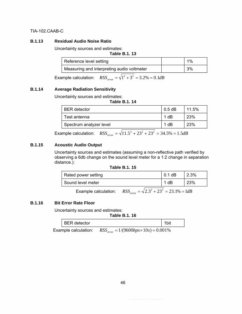
TIA-102.CAAB-C

46

B.1.13 Residual Audio Noise Ratio Uncertainty sources and estimates:

Table B.1. 13

Reference level setting 1%

Measuring and interpreting audio voltmeter 3%

Example calculation: dBRSSerror 1.0%2.331 22 ==+=

B.1.14 Average Radiation Sensitivity Uncertainty sources and estimates:

Table B.1. 14


Test antenna 1 dB 23%

Spectrum analyzer level 1 dB 23%

Example calculation: dBRSSerror 5.1%5.3423235.11 222 ==++=

B.1.15 Acoustic Audio Output Uncertainty sources and estimates (assuming a non-reflective path verified by observing a 6db change on the sound level meter for a 1:2 change in separation distance.):

Table B.1. 15

Rated power setting 0.1 dB 2.3%

Sound level meter 1 dB 23%

Example calculation: dBRSSerror 1%1.23233.2 22 ==+=

B.1.16 Bit Error Rate Floor Uncertainty sources and estimates:

Table B.1. 16

BER detector 1bit Example calculation: %001.0)109600/(1 =×= sbpsRSSerror

--```,``,,`,,``,```,`````,`````-`-`,,`,,`,`,,`---

TIA-102.CAAB-C

47

B.1.17 Late Entry Unsquelch Delay Uncertainty sources and estimates (for a receiver with a late entry unsquelch delay of 100 ms):

Table B.1. 17

Oscilloscope delta time base 410 μ s 0.4%

Switch closure 10 ms 10%

Example calculation: %10104.0 22 =+=errorRSS = 10 ms.

B.1.18 Receiver Throughput Delay Uncertainty sources and estimates (for a receiver with a throughput delay of 100 ms):

Table B.1. 18


Time for test tone appearance second output signal transition

10 ms 10%

Example calculation (for a receiver with a throughput delay of 100 ms):

%10104.0 22 =+=errorRSS = 10 ms.

--```,``,,`,,``,```,`````,`````-`-`,,`,,`,`,,`---

TIA-102.CAAB-C

48

B.2 Example Calculations for Transmitter Measurements B.2.1 RF Output Power

Uncertainty sources and estimates (for a 25 watt transmitter): Table B.2. 1

Power meter/sensor: reference level 2% 2%

Calibration mismatch 8.686 x rg x rl = 8.686 x 0.029 x 0.091

0.023 dB 0.5%

Sensor calibration factor 2.3% 2.3%

Range-to-range change (one range change) 0.02 dB 0.5%

Meter linearity 0.02 dB 0.5%

Meter zero 0.02 dB 0.5%

Mismatch transmitter load 8.686 x rTX x rLI = 8.686 x 0.33 x 0.091

0.26 dB 6.0%

Mismatch load power sensor 8.686 x rLO x rSI = 8.686 x 0.091 x 0.091

0.072 dB 1.76%

Load attenuation (can be reduced if the attenuator is calibrated at the transmitter's frequency)

0.5 dB 11.5%

Power supply contribution, @ 13.8 V 0.25 dB/V x 0.007V

0.02 dB 0.5%

Example calculation:

dBRSSerror 59.0%5.135.117.165.053.22 222222 ==+++×++= Note: RSS error = 13.4% (0.58 dB) for 25 mW (+14 dBm) into the power sensor.

B.2.2 Operating Frequency Accuracy Uncertainty sources and estimates error (based on a frequency of 550 MHz):

Table B.2. 2

Timebase (based on counter calibration cycle of 30 days), timebase drift x 30 days x 550 MHz = 10-9 x 30 x 550x106

16.5 Hz

Counter resolution 1 Hz

Example calculation: HzRSSerror 5.1615.16 22 =+=

--```,``,,`,,``,```,`````,`````-`-`,,`,,`,`,,`---

TIA-102.CAAB-C

49

B.2.3 Electrical Audio Performance Uncertainty sources and estimates error:

Table B.2. 3

Distortion meter used to measure the noise output at the standard receiver output

5% of reading

RMS voltmeter used to measure the audio noise source output

2% of reading

Example calculation: %4.525 22 =+=errorRSS of reading

B.2.4 Acoustic Audio Performance Uncertainty sources and estimates error:

Table B.2. 4

Distortion meter used to measure the pink noise output at the standard receiver output

5%

Sound level meter

1 dB 23%

Example calculation: dBRSSerror 0.1%5.23235 22 ==+=

B.2.5 Modulation Emission Spectrum Uncertainty sources and estimates error:

Table B.2. 5

Spectrum analyzer frequency response flatness 0.6 dB 13.8%


Example calculation: dBRSSerror 1.2%1.48468.13 22 ==+=

B.2.6 Radiated Spurious Emissions Uncertainty sources and estimates error:

Table B.2. 6

Substitution antenna position and gain 1 dB 23%

RF signal generator absolute level 1 dB 23%

Mismatch between the signal generator output and the substitution antenna 8.686 x rSO x rAT = 8.686 x 0.091 x 0.33

0.26 dB 6.0%

Standard radiation test site 3.0 dB 69%

--```,``,,`,,``,```,`````,`````-`-`,,`,,`,`,,`---

TIA-102.CAAB-C

50

Example calculation: dBRSSerror 3.3%6.76690.62323 2222 ==+++= Note: The uncertainty of the carrier power measurement needs to be included if the results were recorded as spurious emission attenuation rather than spurious emission power.

B.2.7 Conducted Spurious Emissions Uncertainty sources and estimates error (for a 10 watt transmitter):

Table B.2. 7

Load power coefficient: (assume output VSWR = 2.0:1 into a 30 dB ±0.5 dB load with power factor 0.001 dB/dB x 10W)

0.3 dB 6.9%

Mismatch transmitter ⇒ load 8.686 x rTX x rLI = 8.686 x 0.33 x 0.091

0.26 dB 6.0%

Mismatch load ⇒ notch filter 8.686 x rLO x rFI = 8.686 x 0.091 x 0.091

0.07 dB 1.7%

Mismatch notch filter⇒ spectrum analyzer 8.686 x rFO x rAI = 8.686 x 0.091 x 0.20

0.16 dB 3.6%


Signal generator ⇒ load 8.686 x rSO x rLI = 8.686 x 0.20 x 0.091

0.16 dB 3.6%

Mismatch load⇒ notch filter 8.686 x rLO x rFI = 8.686 x 0.091 x 0.091

0.07 dB 1.7%

Mismatch notch filter ⇒ spectrum analyzer 8.686 x rFO x rAI = 8.686 x 0.091 x 0.20

0.16 dB 3.6%

Example calculation:

dBRSSerror 1.1%6.256.37.16.3236.37.169.6 22222222 ==+++++++= Note: Uncertainty of the carrier power measurement needs to be included if the results were recorded as spurious emission attenuation.

B.2.8 Adjacent Channel Power Ratio Uncertainty sources and estimates error:

Table B.2. 8




--```,``,,`,,``,```,`````,`````-`-`,,`,,`,`,,`---

TIA-102.CAAB-C

51

B.2.9 Intermodulation Attenuation

Uncertainty sources and estimates error: Table B.2. 9

Power measurement (see clause on RF Output Power uncertainty)

0.59 dB 13.5%

20 dB attenuator 0.5 dB 11.5%

Coupler loss 0.5 dB 11.5%

10 dB attenuator 0.5 dB 11.5%

(The above three could be reduced if the path were calibrated)

Interfering signal to the transmitter:

Mismatch of interfering source⇒ 20 dB attenuator 8.686 x rINT x r20 = 8.686 x 0.33 x 0.046

0.13 dB 3.0%

Mismatch of 20 dB att ⇒ coupler 8.686 x r20 x rcplthru = 8.686 x 0.046 x 0.166

0.07 dB 1.5%

Mismatch uncertainty of coupler ⇒ 10 dB atten. 8.686 x rcplthru x r10 = 8.686 x 0.166 x 0.046

0.07 dB 1.5%

Mismatch uncertainty of 10 dB att ⇒ transmitter 8.686 x r10 x rTX = 8.686 x 0.0.046 x 0.33

0.13 3.0%

Assume that the above uncertainty in the interfering signal will have a 1 dB/ 1 dB effect on the intermodulation product.

Signals to the spectrum analyzer:

Mismatch of transmitter ⇒ 10 dB attenuator 8.686 x rTX x r10 = 8.686 x 0.33 x 0.046

0.13 dB 3.0%

Mismatch of 10 dB att ⇒ coupler 8.686 x r10 x rcplthru = 8.686 x 0.046 x 0.166

0.07 dB 1.5%

Mismatch of coupler ⇒ spectrum analyzer 8.686 x rcplau x rA = 8.686 x 0.23 x 0.20

0.4 dB 9.2%


Spectrum analyzer log fidelity amplitude 2 dB 46.1% Example calculation:

dBRSSerror 4.2%9.541.468.132.95.130.335.1135.13 2222222 ==+++×+×+×+=

--```,``,,`,,``,```,`````,`````-`-`,,`,,`,`,,`---

TIA-102.CAAB-C

52

B.2.10 Average Radiated Power Output Uncertainty sources and estimates error:

Table B.2. 10

Substitution antenna position and gain 1 dB 23%

Mismatch between the signal generator output and the substitution antenna 8.686 x rSO x rAT = 8.686 x 0.091 x 0.33

0.26 dB 6.0%

RF signal generator absolute level 1 dB 23%

Radiation test site 3.0 dB 69%

Example calculation: dBRSSerror 3.3%6.7669230.623 2222 ==+++=

B.2.11 Conducted Spurious Emissions into VSWR Uncertainty sources and estimates error:

Table B.2. 11

Mismatch of signal generator ⇒ load 8.686 x rSO x rCPLR/TERM = 0.686 x 0.091 x 0.091

0.07 dB 1.6%

Signal generator 1 dB 23%


B.2.12 Transmitter Power and Encoder Attack Time Uncertainty sources and estimates (for a transmitter with an approximate attack time of 100 ms)

Table B.2. 12


Switch closure 10 ms 10%

Example calculation: msRSSerror 10%10104.0 22 ==+= B.2.13 Transmitter Power and Encoder Attack Time with Busy/Idle Operation

Uncertainty sources and estimates (for a transmitter with an attack time of 100 ms) Table B.2. 13


Example calculation: sRSSerror μ=== 410%4.04.0 2

--```,``,,`,,``,```,`````,`````-`-`,,`,,`,`,,`---

TIA-102.CAAB-C

53

B.2.14 Transmitter Throughput Delay Uncertainty sources and estimates (for a transmitter with an attack time of 100 ms)

Table B.2. 14

Oscilloscope delta timebase 410 μ s 0.4%


B.2.15 Frequency Deviation for C4FM Uncertainty sources and estimates:

Table B.2. 15

FM demodulator deviation 1%

B.2.16 Modulation Fidelity Uncertainty sources and estimates: a) Combined C4FM and CQPSK method carrier offset:

Table B.2. 16

Carrier offset of the modulation fidelity measuring system

10 Hz 0.6%

Example calculation: HzRSSerror 10%6.06.0 2 === Table B.2. 16A

RMS deviation of the modulation fidelity measuring system

5%

Example calculation: %552 ==errorRSS b) C4FM only method:

Table B.2. 16B

RF FM signal generator 5%

FFT spectrum analyzer level 5%

FFT spectrum analyzer phase 5%

Example calculation: %7.853 2 =×=errorRSS

--```,``,,`,,``,```,`````,`````-`-`,,`,,`,`,,`---

TIA-102.CAAB-C

54

B.2.17 Symbol Rate Accuracy Uncertainty sources and estimates based on a 1200 symbol per second pattern:

Table B.2. 17

Time base uncertainty based on a counter calibration cycle of 30 days Time base drift x 30 days x 1200 Hz = 10-9x30x1200

3.6x10-5 Hz

Counter resolution (±1 count) 1x10-6 Hz Example calculation:

PPMHzRSSerror 03.0105.3)101()106.3( 52625 =×=×+×= −−−

B.2.18 Transient Frequency Behavior a) FM demodulator method: Uncertainty sources and estimates based on a 5 ms timing measurement:

Table B.2. 18A

Uncertainty of FM demodulator capture 1 ms 20%

Oscilloscope delta time base uncertainty 410 μ s 8.2%

Example calculation: ms1.1%6.2122.8220errorRSS ==+= b) Modulation domain analyzer method: Uncertainty sources and estimates based on a 5 ms timing measurement:

Table B.2. 18B

Modulation domain analyzer delta time resolution 44 µs 0.9%


B.2.19 RFSS Throughput Delay Uncertainty sources and estimates based on a 100 ms throughput delay:

Table B.2. 19

Calibrated receiver delay 14 ms 14%


Example calculation: msRSSerror 14%144.014 22 ==+=

--```,``,,`,,``,```,`````,`````-`-`,,`,,`,`,,`---

TIA-102.CAAB-C

55

B.2.20 RFSS Idle to Busy Transition Time Uncertainty sources and estimates based on a 100 ms transition time:

Table B.2. 20


Oscilloscope resolution 50 ps 0%

Example calculation: sRSSerror μ410%4.04.0 2 ===

--```,``,,`,,``,```,`````,`````-`-`,,`,,`,`,,`---

TIA-102.CAAB-C

56

B.3 Trunking System Measurements The examples in this section are for the limits in Section 3.3 using the methods of measurement in Section 2.3 of ANSI/TIA/EIA-102.CAAA.

B.3.1 Trunking Control Channel Slot Times Uncertainty sources and estimates based on a 100 ms slot time:

Table B.3 1


B.3.2 Trunking Request Time

Uncertainty sources and estimates based on a 100 ms trunking request time: Table B.3 2


B.3.3 Trunking Voice Access Time

Uncertainty sources and estimates based on a 100 ms trunking voice access time: Table B.3 3


B.3.4 Time to Grant

Uncertainty sources and estimates based on a 100 ms time to grant: Table B.3 4


B.3.5 Transmitter Time to Key on a Traffic Channel

Uncertainty sources and estimates based on a 100 W transmitter time to key on a traffic channel:

Table B.3 5

Oscilloscope delta time base 410 μ s 0.4% --```,``,,`,,``,```,`````,`````-`-`,,`,,`,`,,`---

TIA-102.CAAB-C

57

BIBLIOGRAPHY (informative) EIA/TIA – 603 –1993, Land mobile FM or PM communications equipment and performance standards. Murphy, R. B. On the Meaning of Precision and Accuracy, NBS Special Publication 300, Vol. 1, February 1969, pp. 357-360. Eisenhart, C. Realistic Evaluation of the Precision and Accuracy of Instrument Calibration Systems, NBS Special Publication 300, Vol. 1, February 1969, pp. 21-47. Eisenhart, C. Expression of the Uncertainties of Final Results, NBS Special Publication 300, Vol. 1, February 1969, pp. 69-72. Ku, H. H. Notes of the Use of Propagation of Error Formulas, NBS Special Publication 300, Vol. 1, February 1969, pp. 73-78. Dorsey, N. E. and Eisenhart, C. On Absolute Measurement, NBS Special Publication 300, Vol. 1, February 1969, pp. 49-55. Hewlett-Packard Application note 64-1, Fundamentals of RF and Microwave Power Measurements August 1977, pp. 29-34.

--```,``,,`,,``,```,`````,`````-`-`,,`,,`,`,,`---

--```,``,,`,,``,```,`````,`````-`-`,,`,,`,`,,`---