lane keeping and navigation assist system - yash sharma · lane keeping and navigation assist...
TRANSCRIPT
Lane Keeping and Navigation Assist System
Yash SharmaAlbert Nerken School of Engineering
The Cooper Union
Vishnu KaimalAlbert Nerken School of Engineering
The Cooper Union
Abstract
We built a miniature autonomous vehicle which can navigate through maps consist-
ing of various road topologies. Our system is comprised of a perception module,
for detecting lanes and intersections, and a control module, for lane keeping and
turn making. A map was constructed for validation, and we have verified that our
vehicle can navigate while keeping within the lane lines. This report details the
background necessary for understanding our project, related work similar to ours
proposed by researchers, and the details of our approach.

Contents
1 Introduction 1
2 Background 2
2.1 DARPA Challenges . . . . . . . . . . . . . . . . . . . . . . . . . . . . . . . . . . 2
2.1.1 Beyond DARPA . . . . . . . . . . . . . . . . . . . . . . . . . . . . . . . 2
2.2 Perception . . . . . . . . . . . . . . . . . . . . . . . . . . . . . . . . . . . . . . . 3
2.2.1 Camera Calibration . . . . . . . . . . . . . . . . . . . . . . . . . . . . . . 4
2.2.2 Perspective Transform . . . . . . . . . . . . . . . . . . . . . . . . . . . . 5
2.2.3 Edge Detection . . . . . . . . . . . . . . . . . . . . . . . . . . . . . . . . 6
2.2.4 Deep Learning . . . . . . . . . . . . . . . . . . . . . . . . . . . . . . . . 9
2.3 Sensors . . . . . . . . . . . . . . . . . . . . . . . . . . . . . . . . . . . . . . . . 13
2.3.1 Sensor Fusion . . . . . . . . . . . . . . . . . . . . . . . . . . . . . . . . . 14
2.3.2 Localization . . . . . . . . . . . . . . . . . . . . . . . . . . . . . . . . . . 16
2.3.3 Mapping . . . . . . . . . . . . . . . . . . . . . . . . . . . . . . . . . . . 16
2.4 Vehicle . . . . . . . . . . . . . . . . . . . . . . . . . . . . . . . . . . . . . . . . 17
2.4.1 Differential Steering . . . . . . . . . . . . . . . . . . . . . . . . . . . . . 17
2.4.2 2-Wheel Drive . . . . . . . . . . . . . . . . . . . . . . . . . . . . . . . . 18
2.5 Control . . . . . . . . . . . . . . . . . . . . . . . . . . . . . . . . . . . . . . . . 18
2.5.1 PID Controller . . . . . . . . . . . . . . . . . . . . . . . . . . . . . . . . 18
2.5.2 Model Predictive Control . . . . . . . . . . . . . . . . . . . . . . . . . . . 20
2.6 Planning . . . . . . . . . . . . . . . . . . . . . . . . . . . . . . . . . . . . . . . . . 21
2.6.1 Environmental Prediction . . . . . . . . . . . . . . . . . . . . . . . . . . . 21
2.6.2 Behavior Planning . . . . . . . . . . . . . . . . . . . . . . . . . . . . . . . 21
2.6.3 Trajectory Generation . . . . . . . . . . . . . . . . . . . . . . . . . . . . 22
2.6.4 Reinforcement Learning . . . . . . . . . . . . . . . . . . . . . . . . . . . 22
3 Related Work 23
4 Project Description 26
4.1 Lane Keeping System . . . . . . . . . . . . . . . . . . . . . . . . . . . . . . . . . 26
4.1.1 Perception Module . . . . . . . . . . . . . . . . . . . . . . . . . . . . . . 26
4.1.2 Control Module . . . . . . . . . . . . . . . . . . . . . . . . . . . . . . . . 28
4.2 Navigation System . . . . . . . . . . . . . . . . . . . . . . . . . . . . . . . . . . 28
4.2.1 Intersections . . . . . . . . . . . . . . . . . . . . . . . . . . . . . . . . . 29
4.3 Software Architecture . . . . . . . . . . . . . . . . . . . . . . . . . . . . . . . . . 30
5 Results and Evaluation 30
5.1 Experimental Setup . . . . . . . . . . . . . . . . . . . . . . . . . . . . . . . . . . 30
5.1.1 Vehicle . . . . . . . . . . . . . . . . . . . . . . . . . . . . . . . . . . . . 30
5.1.2 Lane Configurations . . . . . . . . . . . . . . . . . . . . . . . . . . . . . 32
5.1.3 Navigation Map . . . . . . . . . . . . . . . . . . . . . . . . . . . . . . . 32
5.2 Results . . . . . . . . . . . . . . . . . . . . . . . . . . . . . . . . . . . . . . . . . 33
6 Conclusion 34
1 Introduction
The possibility of self-driving cars has fascinated us for decades now, but only recently have they
appeared to be an impending reality. By 2007, with the final DARPA Urban Challenge finishing in a
success, the seeds were planted for research in this field, and now the first commercial self-driving
cars appear to be close to market. Google, Tesla, Uber, and other large players in this space, already
have self-driving vehicles navigating through neighborhoods. At this point, the tasks remaining for
such companies are building self-driving vehicles with inexpensive equipment such that they can
be viable commercial products, and convincing the market of the safety of such systems, as one
malfunction could result in death.
Despite the progress that has been made in the field, little public research is available, as most
researchers working on this topic are in industry, aiming to beat their competitors in bringing an
autonomous vehicle to the market. This makes the project of building a self-driving car one ripe with
exploration. Therefore, we have decided to test in a controlled environment, so real-world complexity
can be added for experimentation and not ever-present, making the project inviable.
In order to get started in building self-driving cars, understanding the history of the field is important,
as it details the direction for future work. In the background section, we will discuss the DARPA
Challenges, and how self-driving car research has progressed since then. We then will discuss the
modern approaches to perception, sensor fusion, control, and planning. We will also discuss pertinent
information needed for understanding such approaches, such as machine learning, kalman filters, and
differential steering. In the related work section, we will discuss public research work, which has
mainly been focused on how artificial intelligence, principally deep learning, can be used to solve
self-driving cars’ most difficult problems.
We will then describe our project: a lane keeping and navigation assist system. We will first describe
our experimental setup: our vehicle, lane configurations, and navigation map. We will then discuss
our approach, which consists of perception and control submodules wrapped in a multithreaded
software architecture. We will discuss our current results, both quantitative and qualitative, and
finally, we will discuss possible future work, thus concluding our report.
1
2 Background
In this section, we will discuss the history of self-driving car research, particularly the DARPA
challenges, which jump-started the field. We will then explain the techniques underlying the modern
self-driving car’s key subsystems: perception, sensors, the vehicle model, control, and planning.
2.1 DARPA Challenges
Self-driving cars are quite a hot topic nowadays, as nearly every automaker, tech company, and a
flock of startups are rushing to colonize an industry that has the potential to save tens of thousands of
lives, and generate trillions of dollars. What is shocking is how far we’ve come in the past ten years,
since the Defense Advanced Research Projects Agency, better known as DARPA, hosted their first
urban challenge for developing driverless cars.
The first competition was hosted in 2004, where every vehicle crashed, failed, or caught fire, most
of them in sight of the starting line. However, the competition ignited a community of people
interested in building this technology, and thus a second competition was hosted in 2005. Here, the
top-performing vehicle was from Stanford University, built by the Stanford Racing Team led by
Sebastien Thrun, and the basis for its functionality was machine learning. The vehicle, called Stanley,
was trained for generating appropriate speeds and steering angles, given the environmental state, in
order to safely and efficiently navigate across a desert. This use of artificial intelligence set the stage
for learning techniques to dominate recent research in solving autonomous vehicles’ most difficult
questions [31].
For the final DARPA challenge, hosted in 2007, a more realistic environment was used, an urban
environment with multiple vehicles navigating simultaneously. Various tasks were given, such as
executing three-point turns, parking and more, while constraining the vehicles to not crash into other
vehicles and obey California’s driving rules. The results were widely successful; 6 teams ended up
fully finishing the challenge. This time around, CMU’s “Boss” defeated Stanford’s “Junior” and
placed first [32, 25].
With the success of this final urban challenge, the community was convinced self-driving vehicles
will become a reality in the near future. However, significant hurdles would have to be overcome to
achieve the urban challenge’s encouraging results in the real world.
2.1.1 Beyond DARPA
As can be seen in Figure 1, a typical vehicle in the DARPA challenge carried multiple LIDARs,
Radars, a highly sensitive IMU, and computing power of a dozen computers [32]. Moreover, an
2
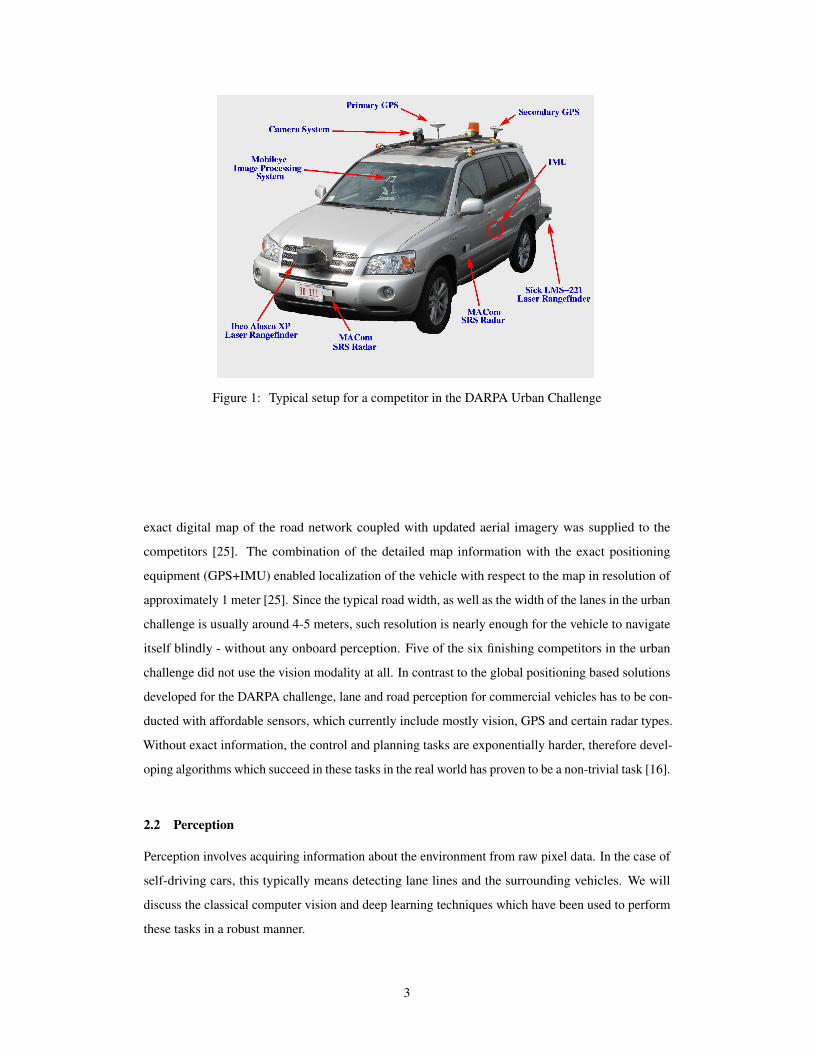
Figure 1: Typical setup for a competitor in the DARPA Urban Challenge
exact digital map of the road network coupled with updated aerial imagery was supplied to the
competitors [25]. The combination of the detailed map information with the exact positioning
equipment (GPS+IMU) enabled localization of the vehicle with respect to the map in resolution of
approximately 1 meter [25]. Since the typical road width, as well as the width of the lanes in the urban
challenge is usually around 4-5 meters, such resolution is nearly enough for the vehicle to navigate
itself blindly - without any onboard perception. Five of the six finishing competitors in the urban
challenge did not use the vision modality at all. In contrast to the global positioning based solutions
developed for the DARPA challenge, lane and road perception for commercial vehicles has to be con-
ducted with affordable sensors, which currently include mostly vision, GPS and certain radar types.
Without exact information, the control and planning tasks are exponentially harder, therefore devel-
oping algorithms which succeed in these tasks in the real world has proven to be a non-trivial task [16].
2.2 Perception
Perception involves acquiring information about the environment from raw pixel data. In the case of
self-driving cars, this typically means detecting lane lines and the surrounding vehicles. We will
discuss the classical computer vision and deep learning techniques which have been used to perform
these tasks in a robust manner.
3

Figure 2: Two common forms of radial distortion: barrel distortion and pincushion distortion
2.2.1 Camera Calibration
With the introduction of cheap, pinhole cameras in the late 20th century, cameras became a common
occurence in our everyday life. Unfortunately, this cheapness comes with a price, significant distortion.
Two major distortions which are introduced are radial distortion and tangential distortion.
Radial distortion is radially symmetric, or approximately so, arising from the symmetry of a pho-
tographic lens. An example of radial distortion can be seen in Figure 2. Due to radial distortion,
straight lines will appear curved. Positive radial distortion, barrel distortion, induces the visible effect
where lines which do not go through the center of the image are bowed outwards, away from the
center. On the other hand, negative radial distortion, pincushion distortion, forces such lines to bow
inwards, towards the center of the image. This distortion is represented as follows:
xdistorted = x(1 + k1r2 + k2r
4 + k3r6
ydistorted = y(1 + k1r2 + k2r
4 + k3r6
where ki are radial distortion coefficients [35]. Similarly, tangential distortion occurs because image-
taking lenses are not aligned perfectly parallel to the imaging plane. So, some areas in the image may
look nearer than expected. This is represented as below:
xdistorted = x+ [2p1xy + p2(r2 + 2x2)]
ydistorted = y + [2p2xy + p1(r2 + 2y2)]
where pi are tangential distortion coefficients. Therefore, the goal is to find these radial and tangential
distortion coefficients. However, the extrinsic and intrinsic parameters of the camera need to be
determined. Extrinsic parameters correspond to rotation and translation vectors which translates the
coordinates of a 3D point to a coordinate system. Intrinsic parameters are specific to the camera, such
as information like focal length (fx, fy) and optical centers (cx, cy).
4
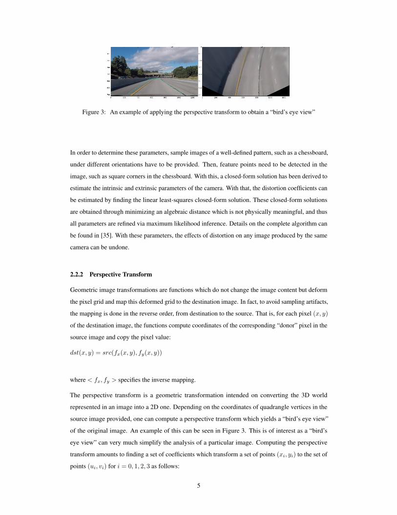
Figure 3: An example of applying the perspective transform to obtain a “bird’s eye view”
In order to determine these parameters, sample images of a well-defined pattern, such as a chessboard,
under different orientations have to be provided. Then, feature points need to be detected in the
image, such as square corners in the chessboard. With this, a closed-form solution has been derived to
estimate the intrinsic and extrinsic parameters of the camera. With that, the distortion coefficients can
be estimated by finding the linear least-squares closed-form solution. These closed-form solutions
are obtained through minimizing an algebraic distance which is not physically meaningful, and thus
all parameters are refined via maximum likelihood inference. Details on the complete algorithm can
be found in [35]. With these parameters, the effects of distortion on any image produced by the same
camera can be undone.
2.2.2 Perspective Transform
Geometric image transformations are functions which do not change the image content but deform
the pixel grid and map this deformed grid to the destination image. In fact, to avoid sampling artifacts,
the mapping is done in the reverse order, from destination to the source. That is, for each pixel (x, y)
of the destination image, the functions compute coordinates of the corresponding “donor” pixel in the
source image and copy the pixel value:
dst(x, y) = src(fx(x, y), fy(x, y))
where < fx, fy > specifies the inverse mapping.
The perspective transform is a geometric transformation intended on converting the 3D world
represented in an image into a 2D one. Depending on the coordinates of quadrangle vertices in the
source image provided, one can compute a perspective transform which yields a “bird’s eye view”
of the original image. An example of this can be seen in Figure 3. This is of interest as a “bird’s
eye view” can very much simplify the analysis of a particular image. Computing the perspective
transform amounts to finding a set of coefficients which transform a set of points (xi, yi) to the set of
points (ui, vi) for i = 0, 1, 2, 3 as follows:
5

ui =a0xi+a1yi+a2
c0xi+c1yi+1
vi =b0xi+b1yi+b2c0xi+c1yi+1
The eight coefficients can be calculated by solving the following linear system:
x0 y0 1 0 0 0 −x0u0 −y0u0x1 y1 1 0 0 0 −x1u1 −y1u1x2 y2 1 0 0 0 −x2u2 −y2u2x3 y3 1 0 0 0 −x3u3 −y3u30 0 0 x0 y0 1 −x0v0 −y0v00 0 0 x1 y1 1 −x1v1 −y1v10 0 0 x2 y2 1 −x2v2 −y2v20 0 0 x3 y3 1 −x3v3 −y3v3
a0
a1
a2
a3
b0
b1
b2
b3
=
u0
u1
u2
u3
v0
v1
v2
v3
There are many available software packages for solving linear systems of equations efficiently. The
solution to this system yields the perspective transform [30].
2.2.3 Edge Detection
Edge detection includes a variety of mathematical methods that aim at identifying points in a digital
image at which the image brightness changes sharply or, more formally, has discontinuities. The
points at which image brightness changes sharply are typically organized into a set of curved line
segments termed edges.
The purpose of detecting sharp changes in image brightness is to capture important events and
changes in properties of the world. In the ideal case, the result of applying an edge detector to an
image may lead to a set of connected curves that indicate the boundaries of objects, the boundaries of
surface markings as well as curves that correspond to discontinuities in surface orientation. Thus,
applying an edge detection algorithm to an image may significantly reduce the amount of data to
be processed and may therefore filter out information that may be regarded as less relevant, while
preserving the important structural properties of an image. If the edge detection step is successful,
the subsequent task of interpreting the information contents in the original image may therefore be
substantially simplified.
Most edge detection algorithms operate upon grayscale images, however there are methods to do
color edge detection, the simplest of which, called the output fusion method, applies edge detectors
6

Figure 4: Example of Sobel edge detector
to the three color channels (RGB or HSV) independently, then combines the results using a logical
operation. Some approaches apply various color transformations, such as converting to the LAB
or HLS colorspaces, then combining edge detection results on pertinent channels in each of the
spaces. There are also more sophisticated methods, called multi-dimensional gradient methods, which
treat the three channels as coordinates of the 3D color space, and try to find edges by analyzing the
gradient [5]. However, most practical applications convert the color images to grayscale, as the color
information is deemed unimportant for edge detection.
The basis for any edge detection algorithm are the intensity gradients of the image. The Sobel edge
detector makes use of two 3x3 convolution kernels [20]. Each is used to approximate a change in the
gradient along the vertical and horizontal axis. After convolving each of these kernels with a matrix
representation of the image, the values Gx and Gy , which represent the gradient along the horizontal
and vertical axis respectively, are calculated for each individual point of the image.
After obtaining the values Gx and Gy for each point of the image, the magnitude of the gradient
is then calculated as |G| =√G2
X +G2y. Next the angle of orientation of each point is calculated
as being θ = arctan(Gx/Gy) [20]. Thus, once the gradients are calculated, this can now be used
to identify edges. Points where the gradient is very high can be labeled as edges and those with
low gradients are not. However, the threshold for this gradient is very important. This is a user
defined parameter that will have to be defined based on the environment variables. For example, for
lane detection, the threshold has to be set such the lane markers have to be identified. This can be
quite difficult since the threshold would have to take into account various types of lanes in different
settings [23].
An example of the Sobel operator at work is shown in Figure 4 [2]. You can see that the outline of
the lanes and terrain in the background are identified clearly. Because there is a significant gradient
7
difference between the the lanes and the dark roads, the Sobel operator is able to easily find these
edges and extract these features for further processing.
A commonly discussed issue with the Sobel operator is that it is an approximation. Because the
pixels on an image are discrete, it is not possible to obtain a continuous gradient along the contours
of the image. Therefore, the smoothing that occurs through the convolution operations from before
are essentially approximations. While this may be true, the performance of this method is still quite
robust. This is mainly because gradient drops are not typically continuous either [20].
Besides the Sobel operator, another commonly used method for edge detection is Canny edge
detection [7]. Again, just like Sobel, Canny looks at gradient differences in the image to detect edges.
However, unlike the Sobel operator, Canny has a complicated pipelined process that one has to follow
to detect edges.
The first step in Canny edge detection is to remove any noise. Again, because we are looking for
gradient differences, any significant gradient drop will be picked up. Therefore, there may be isolated
pixels where the gradient drops off suddenly. To remove such noise from an image, Canny first
convolves the image with a Gaussian filter. This is typically known as applying a Gaussian blur. This
smooths the image by blurring the image. Therefore, the isolated pixels that have gradient drops
won’t be picked up at later stages.
Following this application of a Gaussian blur, the next step is to find the intensity gradients of the
image. This process is exactly the same as that which was described previously for the Sobel operator.
The magnitude of the the gradient is found by convolving a Sobel kernel with the image.
Once the intensity gradients are found at each pixel, the next step removes any unwanted pixels from
the image. This is done by using a technique called non-maximum suppression. Here, each pixel is
checked to see whether it is a local minimum in the direction of the gradient. If this is not the case,
the pixel value is set to zero. This process is intended to find connected pixels that may form an edge
within the image and to suppress any pixels that are otherwise not.
The final step in this process is thresholding. A minimum and maximum value for the gradient
are entered as parameters. Any pixel whose gradient is above the max threshold is automatically
categorized as a pixel and any pixel whose gradient is below the min threshold is categorized as not
a pixel. However, what makes Canny edge detection so robust is the fact that that it also considers
the connectivity of pixels. So, if there is a connected line of pixels in which some of the pixels
are between the minimum and maximum threshold, then all the pixels in that connected line are
categorized as edges. Other techniques simply classify an edge using one threshold [7].
8

Figure 5: Example of Canny edge detector
Shown in Figure 13 is an example of Canny edge detection for extracting features from an image with
lanes [4]. It is effective in identifying the edges of the lanes as well as the dash marks. What makes
Canny edge detection quite unique is that it can work in any environment, because of its effectiveness
in reducing noise in the image.
2.2.4 Deep Learning
A machine learning algorithm is an algorithm that is able to learn from data. The central challenge of
machine learning is to not just perform well on the data at hand, but to also perform well on new,
previously unseen inputs. This task is called generalization. Typically, when training a machine
learning model, we have access to a training set, we can compute some error measure on the training
set called the training error, and we reduce this training error. So far, what we have described is
simply an optimization problem. What separates machine learning from optimization is that we
want the generalization error, also called the test error, to be low as well. The generalization error
is defined as the expected value of the error on a new input. Here the expectation is taken across
different possible inputs, drawn from the distribution of inputs we expect the system to encounter in
practice. We typically estimate the generalization error of a machine learning model by measuring its
performance on a test set of examples that were collected separately from the training set.
The factors determining how well a machine learning algorithm will perform are its ability to 1) make
the training error small, and 2) make the gap between the training and test error small. These two
factors correspond to the two central challenges in machine learning: underfitting and overfitting.
Underfitting occurs when the model is not able to obtain a sufficiently low error value on the training
set. Overfitting occurs when the gap between the training error and test error is too large. We can
control whether a model is more likely to overfit or underfit by altering its capacity. Informally,
a model’s capacity is its ability to fit a wide variety of functions. Models with low capacity may
struggle to fit the training set. Models with high capacity can overfit by memorizing properties of the
training set that do not serve them well on the test set. Machine learning algorithms will generally
perform best when their capacity is appropriate for the true complexity of the task they need to
perform and the amount of training data they are provided with. Models with insufficient capacity are
9
unable to solve complex tasks. Models with high capacity can solve complex tasks, but when their
capacity is higher than needed to solve the present task they may overfit.
Learning theory claims that a machine learning algorithm can generalize well from a finite training
set of examples. This seems to contradict some basic principles of logic. Inductive reasoning, or
inferring general rules from a limited set of examples, is not logically valid. To logically infer a
rule describing every member of a set, one must have information about every member of that set.
In part, machine learning avoids this problem by offering only probabilistic rules, rather than the
entirely certain rules used in purely logical reasoning. Machine learning promises to find rules that
are probably correct about most members of the set they concern. Unfortunately, even this does not
resolve the entire problem. The no free lunch theorem for machine learning states that, averaged
over all possible data generating distributions, every classification algorithm has the same error rate
when classifying previously unobserved points. In other words, in some sense, no machine learning
algorithm is universally any better than any other. The most sophisticated algorithm we can conceive
of has the same average performance (over all possible tasks) as merely predicting that every point
belongs to the same class [34].
Fortunately, these results hold only when we average over all possible data generating distributions.
If we make assumptions about the kinds of probability distributions we encounter in real-world
applications, then we can design learning algorithms that perform well on these distributions. This
means that the goal of machine learning research is not to seek a universal learning algorithm or
the absolute best learning algorithm. Instead, our goal is to understand what kinds of distributions
are relevant to the “real world” that an AI agent experiences, and what kinds of machine learning
algorithms perform well on data drawn from the kinds of data generating distributions we care about.
Supervised learning algorithms are, roughly speaking, learning algorithms that learn to associate some
input with some output, given a training set of examples of inputs x and outputs y. In many cases the
outputs y may be difficult to collect automatically and must be provided by a human “supervisor,”
but the term still applies even when the training set targets were collected automatically. There are
various supervised learning algorithms, such as logistic regression, support vector machines, and
decision trees, which can be used for perception tasks. For example for identifying vehicles in a
dashcam video, a support vector machine can be trained on images of cars and non-cars and then run
a sliding window search on each video frame to identify the location of any cars. However, training a
classifier on raw image data is unnecessary and incredibly computationally expensive. Features have
to be extracted from the images to train such classifiers. Methods to do so include grouping color
features into bins spatially, histograms of color, and the Histogram of Oriented Gradients (HOG)
method [8].
10
The performance of machine learning algorithms depends heavily on the representation of the data
they are given. For example, when logistic regression is used to recommend cesarean delivery, the AI
system does not examine the patient directly. Instead, the doctor tells the system several pieces of
relevant information, such as the presence or absence of a uterine scar. Each piece of information
included in the representation of the patient is known as a feature. Logistic regression learns how
each of these features of the patient correlates with various outcomes. However, it cannot influence
the way that the features are defined in any way. If logistic regression was given an MRI scan of the
patient, rather than the doctor’s formalized report, it would not be able to make useful predictions.
Individual pixels in an MRI scan have negligible correlation with any complications that might occur
during delivery [14].
Many artificial intelligence tasks can be solved by designing the right set of features to extract for
that task, then providing these features to a simple machine learning algorithm. For example, a useful
feature for speaker identification from sound is an estimate of the size of speaker’s vocal tract. It
therefore gives a strong clue as to whether the speaker is a man, woman, or child. However, for
many tasks, it is difficult to know what features should be extracted. For example, in our vehicle
detection example, we know that cars have wheels, so we might like to use the presence of a wheel as
a feature. Unfortunately, it is difficult to describe exactly what a wheel looks like in terms of pixel
values. A wheel has a simple geometric shape but its image may be complicated by shadows falling
on the wheel, the sun glaring off the metal parts of the wheel, the fender of the car or an object in
the foreground obscuring part of the wheel, and so on. The feature extraction methods discussed
previously do a better job than the manual approach described, but are generic in that they don’t adapt
to the specific problem at hand.
One solution to this problem is to use machine learning to discover not only the mapping from
representation to output but also the representation itself. This approach is known as representation
learning [14]. Learned representations often result in much better performance than can be obtained
with hand-designed representations. They also allow AI systems to rapidly adapt to new tasks, with
minimal human intervention. A representation learning algorithm can discover a good set of features
for a simple task in minutes, or a complex task in hours to months. Manually designing features
for a complex task requires a great deal of human time and effort; it can take decades for an entire
community of researchers.
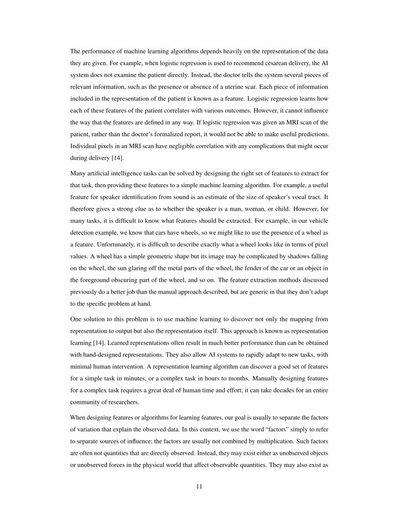
When designing features or algorithms for learning features, our goal is usually to separate the factors
of variation that explain the observed data. In this context, we use the word “factors” simply to refer
to separate sources of influence; the factors are usually not combined by multiplication. Such factors
are often not quantities that are directly observed. Instead, they may exist either as unobserved objects
or unobserved forces in the physical world that affect observable quantities. They may also exist as
11
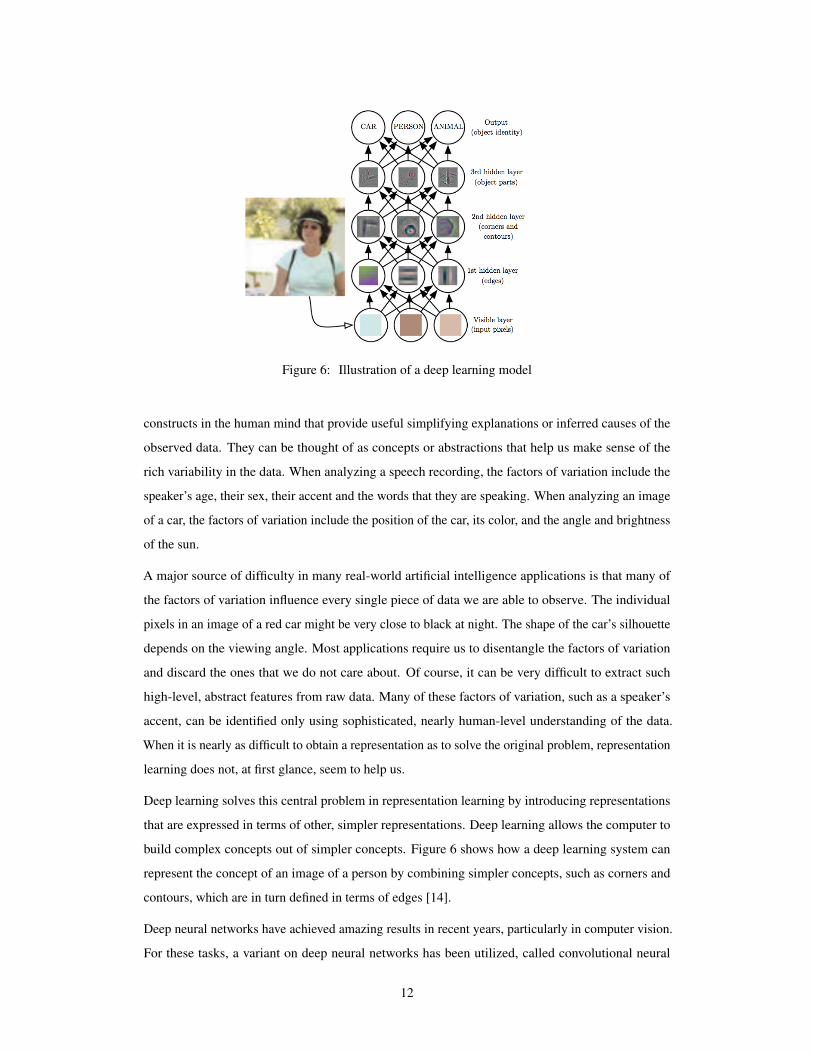
Figure 6: Illustration of a deep learning model
constructs in the human mind that provide useful simplifying explanations or inferred causes of the
observed data. They can be thought of as concepts or abstractions that help us make sense of the
rich variability in the data. When analyzing a speech recording, the factors of variation include the
speaker’s age, their sex, their accent and the words that they are speaking. When analyzing an image
of a car, the factors of variation include the position of the car, its color, and the angle and brightness
of the sun.
A major source of difficulty in many real-world artificial intelligence applications is that many of
the factors of variation influence every single piece of data we are able to observe. The individual
pixels in an image of a red car might be very close to black at night. The shape of the car’s silhouette
depends on the viewing angle. Most applications require us to disentangle the factors of variation
and discard the ones that we do not care about. Of course, it can be very difficult to extract such
high-level, abstract features from raw data. Many of these factors of variation, such as a speaker’s
accent, can be identified only using sophisticated, nearly human-level understanding of the data.
When it is nearly as difficult to obtain a representation as to solve the original problem, representation
learning does not, at first glance, seem to help us.
Deep learning solves this central problem in representation learning by introducing representations
that are expressed in terms of other, simpler representations. Deep learning allows the computer to
build complex concepts out of simpler concepts. Figure 6 shows how a deep learning system can
represent the concept of an image of a person by combining simpler concepts, such as corners and
contours, which are in turn defined in terms of edges [14].
Deep neural networks have achieved amazing results in recent years, particularly in computer vision.
For these tasks, a variant on deep neural networks has been utilized, called convolutional neural
12

networks [22]. Convolutional neural networks emerged from the study of the brain’s visual cortex,
stemming from the observations that many neurons in the visual cortex have small local receptive
field, they only react to visual stimuli located in a limited region of the visual field, and the receptive
fields of different neurons typically overlap, together tiling the whole visual field. Furthermore,
some neurons have larger receptive fields, and react to more complex patterns that are combinations
of the lower-level patterns. Given these biological identifications, convolutional architectures are
typically defined by stacking convolutional layers and pooling layers. Convolutional layers are
partially connected, meaning neurons in the first convolutional layer are only connected to pixels in
their receptive fields. These layers are essentially filters, called convolutional kernels, where each
neuron focuses on low-level features, filtering out all inputs that do not contain said features. During
training, the network finds the most useful filters for its task, and learns to combine them into more
complex patterns. Furthermore, multiple filters are simultaneously applied to the inputs, making
it capable of detecting multiple features anywhere in its input. Pooling layers subsample the input
image in order to reduce the computational load and the number of trainable parameters, thereby
limiting the risk of overfitting.
Convolutional neural networks have become the standard tool for performing image recognition since
2012, when AlexNet was able to trounce the state-of-the-art classical computer vision techniques
in the ImageNet Large-Scale Visual Recognition Challenge, a competition which has been called
the annual "Olympics" for computer vision. 2012 marked the first year where a CNN was used to
achieve a test error rate of 15.4%. The next best entry achieved an error of 26.2% [21, 10]. Since
then, convolutional architectures have grown larger and more complex, achieving amazing results
and remaining computationally tractable due to simultaneous GPU processing optimizations. These
excellent image recognition results have readily transferred over to perception tasks for self-driving
cars.
2.3 Sensors
So far we have discussed perception methods, which are relevant when a camera is used as a sensor
module. However, real-world self-driving vehicles have typically used other sensors, such as LIDAR
and RADAR for executing perception. LIDAR is a light-based RADAR. The sensor sends out short
pulses of invisible laser light, and times how long it takes to see the reflection. From this you learn
both the brightness of the target, and how far away it is, with good accuracy. LIDAR generates a 3-D
map of the world around you, making it easier to detect objects in the presence of others. Furthermore,
LIDAR uses emitted light, so it works independent of the ambient light. Night or day, clouds or sun,
shadows or sunlight, it pretty much sees the same in all conditions. Therefore, despite being very
expensive, multiple LIDARs are currently being used along with camera systems in order to generate
input to the perception module.
13

However, with multiple sensors involved, how does one utilize them all to generate a more accurate
measurement input? Kalman filters are the key mathematical tool for fusing together data, and thus
are discussed in more detail in Section 2.3.1. With sensor fusion results, one can accomplish the
localization task. This is even possible when the map is unknown, by taking the SLAM approach [11].
2.3.1 Sensor Fusion
Kalman filtering is an algorithm that uses a series of measurements observed over time, containing
statistical noise and other inaccuracies, and produces estimates of unknown variables that tend to
be more accurate than those based on a single measurement alone, by estimating a joint probability
distribution over the variables for each timeframe [19]. The algorithm works in a two-step process.
In the prediction step, the Kalman filter produces estimates of the current state variables, along with
their uncertainties. Once the outcome of the next measurement (necessarily corrupted with some
amount of error, including random noise) is observed, these estimates are updated using a weighted
average, with more weight being given to estimates with higher certainty. The algorithm is recursive.
It can run in real time, using only the present input measurements and the previously calculated state
and its uncertainty matrix; no additional past information is required. Using a Kalman filter does
not assume that the errors are Gaussian, however, the filter yields the exact conditional probability
estimate in the special case that all errors are Gaussian-distributed.
The Kalman filter is a recursive estimator. This means that only the estimated state from the previous
time step and the current measurement are needed to compute the estimate for the current state. In
contrast to batch estimation techniques, no history of observations and/or estimates are required. The
Kalman filter can be written as a single equation, however it is most often conceptualized as two
distinct phases: "Predict" and "Update". The predict phase uses the state estimate from the previous
timestep to produce an estimate of the state at the current timestep. This predicted state estimate
is also known as the a priori state estimate because, although it is an estimate of the state at the
current timestep, it does not include observation information from the current timestep. In the update
phase, the current a priori prediction is combined with current observation information to refine the
state estimate. This improved estimate is termed the a posteriori state estimate. Typically, the two
phases alternate, with the prediction advancing the state until the next scheduled observation, and the
update incorporating the observation. However, this is not necessary; if an observation is unavailable
for some reason, the update may be skipped and multiple prediction steps performed. Likewise,
if multiple independent observations are available at the same time, multiple update steps may be
performed [19].
Extensions and generalizations to the method have also been developed, such as the extended Kalman
filter (EKF) and the unscented Kalman filter (UKF) which work on nonlinear systems. The EKF
14
linearizes about an estimate of the current mean and covariance. In the original Kalman filter
formulation, the model assumes the true state at time k is evolved from the state at time (k-1)
according to:
xk = Fkxk−1 +Bkuk + wk
where Fk is the state transition model which is applied to the previous state xk−1, Bk is the control-
input model which is applied to the control vector uk, and wk is the process noise which is assumed
to be drawn from a zero-mean multivariate normal distribution. At time k an observation (or
measurement) zk of the true state xk is made according to:
zk = Hkxk + vk
where Hk is the observation model which maps the true state space into the observed space and
vk is the observation noise which is assumed to be drawn from a zero-mean multivariate normal
distribution. In the EKF formulation, the state transition and observation models don’t need to be
linear functions of the state but may instead be differentiable functions. When the state transition
and observation models are highly non-linear, the extended Kalman filter can give particularly poor
performance. This is because the covariance is propagated through linearization of the underlying non-
linear model. The UKF uses a deterministic sampling technique known as the unscented transform to
pick a minimal set of sample points (called sigma points) around the mean. These sigma points are
then propagated through the non-linear functions, from which a new mean and covariance estimate
are then formed. The result is a filter which, for certain systems, more accurately estimates the true
mean and covariance than EKF [18].
Alternatives to the Kalman filter include the particle filter. Particle filtering uses a genetic mutation-
selection sampling approach, with a set of particles (also called samples) to represent the posterior
distribution of some stochastic process given noisy and/or partial observations. The state-space model
can be nonlinear and the initial state and noise distributions can take any form required. Particle filters
implement the prediction-updating transitions of the filtering equation directly by using a genetic
type mutation-selection particle algorithm. The samples from the distribution are represented by a set
of particles; each particle has a likelihood weight assigned to it that represents the probability of that
particle being sampled from the probability density function [9].
Kalman filters and particle filters are quite related - The Kalman filter bakes the uncertainty into our
best-guess state by representing it as a multidimensional Gaussian, stretching a single belief out to
encompass a large area, whereas the particle filter peppers a number of discrete copies of that best
guess over relatively the same area.
15
2.3.2 Localization
In order to apply the Kalman filter or the particle filter to the tracking task, one needs to incorporate
motion models. The simplest motion model, the constant velocity (CV) model, assumes that, if
a pedestrian is being tracked, the pedestrain will continue to move in that way from one moment
to the next, and any change in that motion, acceleration, is modeled by the “process noise”. The
constant turn rate and velocity (CTRV) model trades the x and y components of the velocity for a
direction and magnitude, and adds in a “yaw rate” component - the change in heading from one
moment to the next. Other motion models include constant turn rate and acceleration (CTRA) and
constant curvature and acceleration (CCA) which introduce additional state parameters. For vehicle
location tracking, researchers find, unsurprisingly, unsurprisingly, that the models perform similarly
for highway driving, but that in an urban setting the more complex motion models outperform the
simpler ones [28].
With a motion model in place, sensor fusion methods can be used to fuse noisy LIDAR data together
to track a pedestrian, or any obstacle from one’s own vehicle’s perspective. Localization involves
finding one’s own uncertain location in a known, mapped area. With known ground truth landmark
locations, LIDAR data representing the observed location of landmarks in relation to the vehicle, and
vehicle control data, these methods can also be applied for solving the localization task.
2.3.3 Mapping
Localizing one’s own vehicle requires knowledge of the environment. In most situations, a known
map is provided; however when one is unavailable, localization can still be done by approaching
the task as a SLAM problem. In robotic mapping and navigation, simultaneous localization and
mapping (SLAM) is the computational problem of constructing or updating a map of an unknown
environment while simultaneously keeping track of an agent’s location within it. Given a series of
sensor observations ot over discrete time steps t, the SLAM problem is to compute an estimate of
the agent’s location xt and a map of the environment mt. Therefore, the objective is to compute
P (mt, xt|o1:t).
Applying Bayes’ rule gives a framework for sequentially updating the location posteriors, given
a map and a transition function P (xt|xt−1). The map can be updated sequentially in a similar
manner. Like many inference problems, the solutions to inferring the two variables together can
be found, to a local optimum solution, by alternating updates of the two beliefs in a form of EM
(expectation-maximization) algorithm. The Kalman filter and Particle filter can be used as statistical
estimation techniques for solving the SLAM problem [11].
16
2.4 Vehicle
Understanding the dynamics of a vehicle is important, especially when operating it for navigation
tasks. Therefore, in this section we will discuss differential steering and the elements of two-wheel
drive.
2.4.1 Differential Steering
The main basis behind differential steering is that there are two separate wheels, each acting inde-
pendently of each other. If both wheels were to spin at the same speed, then the axle that joins these
two wheels would go straight forward at a constant speed. However, if one would wheel were to
spin faster than the other, then this would lead to a differential in rotational speed between the two
wheels.This differential becomes the essence of how an axle turns. Because of the differential, there
is less torque being applied to one side as compared to other. As a result of this, the axle that joins
both wheels follows a radial path in the direction of the slower wheel.
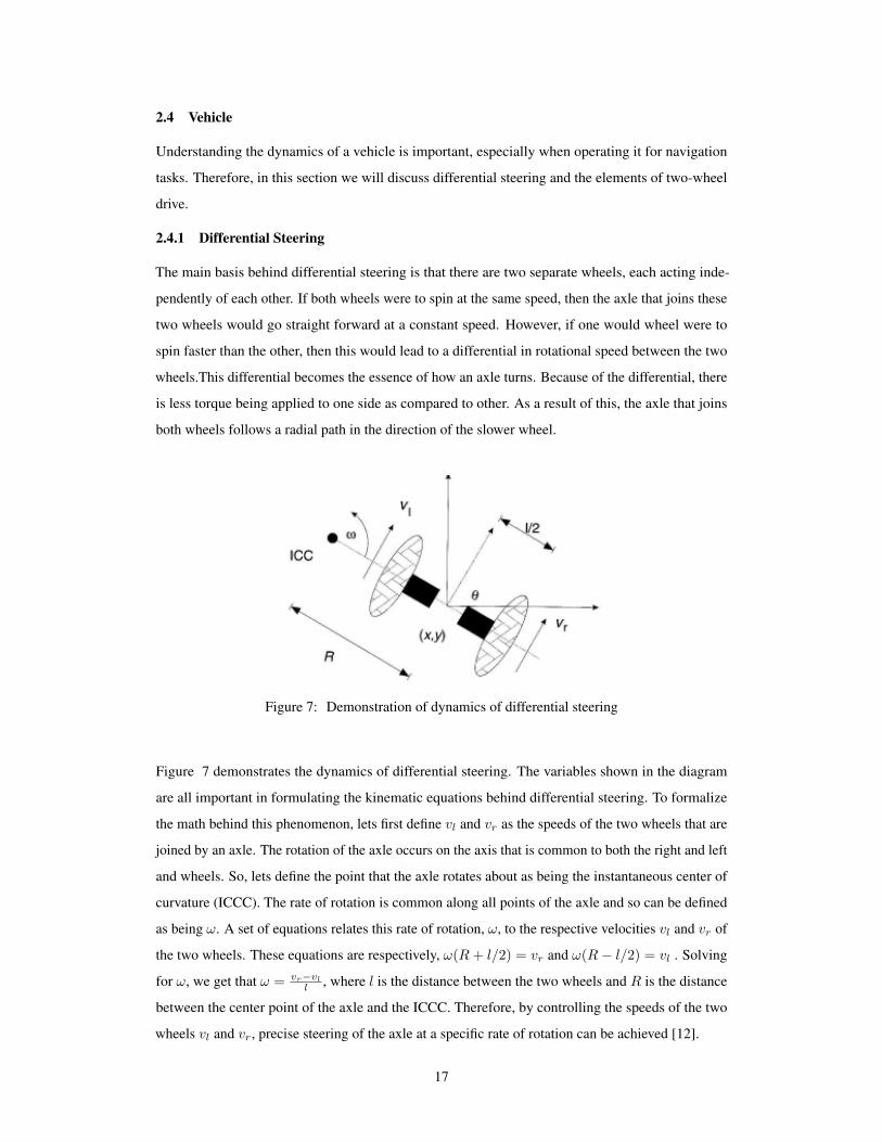
Figure 7: Demonstration of dynamics of differential steering
Figure 7 demonstrates the dynamics of differential steering. The variables shown in the diagram
are all important in formulating the kinematic equations behind differential steering. To formalize
the math behind this phenomenon, lets first define vl and vr as the speeds of the two wheels that are
joined by an axle. The rotation of the axle occurs on the axis that is common to both the right and left
and wheels. So, lets define the point that the axle rotates about as being the instantaneous center of
curvature (ICCC). The rate of rotation is common along all points of the axle and so can be defined
as being ω. A set of equations relates this rate of rotation, ω, to the respective velocities vl and vr of
the two wheels. These equations are respectively, ω(R+ l/2) = vr and ω(R− l/2) = vl . Solving
for ω, we get that ω = vr−vll , where l is the distance between the two wheels and R is the distance
between the center point of the axle and the ICCC. Therefore, by controlling the speeds of the two
wheels vl and vr, precise steering of the axle at a specific rate of rotation can be achieved [12].
17

2.4.2 2-Wheel Drive
A 2-wheel drive vehicle is one in which only two wheels receive power. On a four wheeled vehicle,
a 2-wheel drive provides sufficient traction and is also a simple design to implement. The vehicle
itself can be configured to be either run off the front two wheels or the back two wheels. This is
known as either front-wheel drive or rear-wheel drive. One main advantage of the front-wheel drive
is that it provides better traction. This is because the weight of the engine is balanced by the front
two wheels and thus allows for less slippage. On the other hand one main advantage of a rear-wheel
drive is that there is better balance overall for the vehicle and it also also for better initial acceleration.
The steering mechanism for a 2-wheel drive is implemented with differential steering. Most vehicles
today use what is known as a differential. The differential distributes different levels of power to each
wheel in order to steer [1].
2.5 Control
The control algorithm’s goal is to take the perception and sensor fusion modules’ outputs as input and
yield an actuation where, on average, the difference between the current trajectory and the desired
trajectory is minimized. The PID Controller is the classic closed-loop controller used for this problem,
and will be discussed in more detail below. Model predictive control (MPC), a more sophisticated
control algorithm used for stabilizing the vehicle in a noisy environment, will also be touched on.
2.5.1 PID Controller
The PID controller is a control feedback system that provides automatic control in a variety of
applications. The main advantage of the PID controller, which will be discussed in further detail,
is the precise correction that the controller applies to a system as a result of its use of three compo-
nents. These three components include proportional control, integral control, and derivative control
components. Each of these components allows for the controller to minimize error over time.
It is first important to define how error is calculated within a PID controller. Error is defined as being
the difference between the setpoint and the process variable. The setpoint is the desired or target
value for a specific variable in the system while the process variable is the measured value of a system
process. This defined error term is what the PID controller seeks to minimize and is thus the input
into the three aforementioned components of the controller. The full mathematical form of the PID
controller is defined as being u(t) = Kpe(t) +Ki
∫ t
tie(τ)dτ +Kd
de(t)dt where each of the additive
terms are respectively the proportional, integral, and derivative terms and u(t) represents the output
control variable that should be adjusted. Figure 8 shows the system diagram for the PID controller.
Each of the three components take in the error term as input and are then summed to obtain the
process variable. The output of the system is then fed back in order to calculate the new error at the
next time step.
18
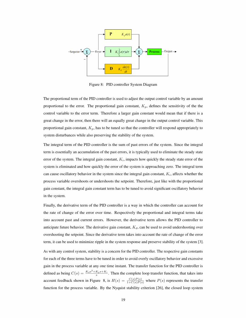
Figure 8: PID controller System Diagram
The proportional term of the PID controller is used to adjust the output control variable by an amount
proportional to the error. The proportional gain constant, Kp, defines the sensitivity of the the
control variable to the error term. Therefore a larger gain constant would mean that if there is a
great change in the error, then there will an equally great change in the output control variable. This
proportional gain constant, Kp, has to be tuned so that the controller will respond appropriately to
system disturbances while also preserving the stability of the system.
The integral term of the PID controller is the sum of past errors of the system. Since the integral
term is essentially an accumulation of the past errors, it is typically used to eliminate the steady state
error of the system. The integral gain constant, Ki, impacts how quickly the steady state error of the
system is eliminated and how quickly the error of the system is approaching zero. The integral term
can cause oscillatory behavior in the system since the integral gain constant, Ki, affects whether the
process variable overshoots or undershoots the setpoint. Therefore, just like with the proportional
gain constant, the integral gain constant term has to be tuned to avoid significant oscillatory behavior
in the system.
Finally, the derivative term of the PID controller is a way in which the controller can account for
the rate of change of the error over time. Respectively the proportional and integral terms take
into account past and current errors. However, the derivative term allows the PID controller to
anticipate future behavior. The derivative gain constant, Kd, can be used to avoid undershooting over
overshooting the setpoint. Since the derivative term takes into account the rate of change of the error
term, it can be used to minimize ripple in the system response and preserve stability of the system [3].
As with any control system, stability is a concern for the PID controller. The respective gain constants
for each of the three terms have to be tuned in order to avoid overly oscillatory behavior and excessive
gain in the process variable at any one time instant. The transfer function for the PID controller is
defined as being C(s) = Kds2+Kps+Ki
s . Then the complete loop transfer function, that takes into
account feedback shown in Figure 8, is H(s) = C(s)P (s)1+C(s)P (s) where P (s) represents the transfer
function for the process variable. By the Nyquist stability criterion [26], the closed loop system
19
maintains stability when |C(s)G(s)| < 1. This criteria ensures that the gain of the system isn’t
excessive and is bounded.
One method for tuning the weights of the PID controller is the Ziegler-Nichols method [36]. This
method follows a specific procedure geared toward each component of the PID controller. First,
the Kd and Ki terms are held to zero. The value of Kp is incrementally increased until the system
response achieves critical gain. Critical gain would mean that the system response is stable and has
oscillations that are bounded and periodic. Once this is achieved, then the Ki and Kd terms are
then adjusted to remove the steady state error and minimize the periodic oscillations in the system’s
response.
What makes the PID Controller easy to use is the fact that the parameters are interpretable, and thus
can be manually tuned. Since each term has a specific role in the system’s response, one can tune the
weights based on the type of behavior they are seeking.
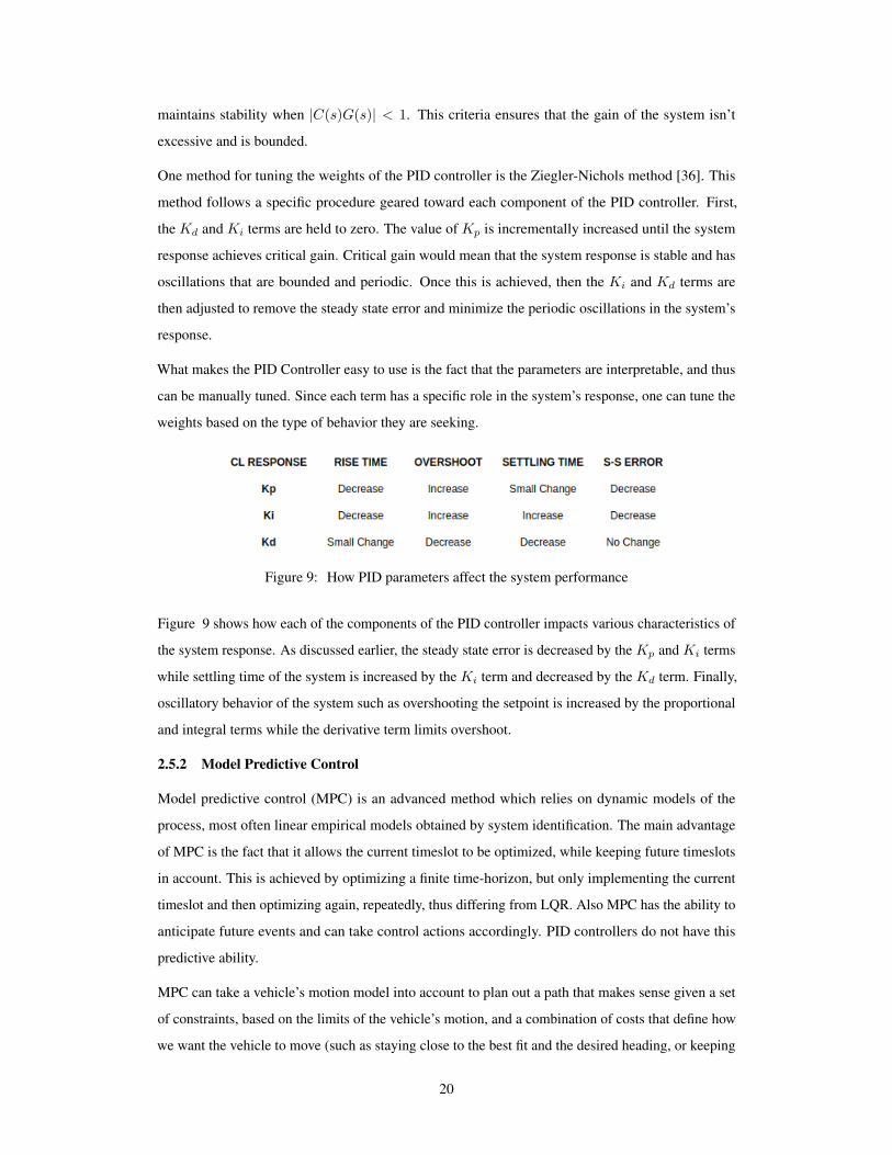
Figure 9: How PID parameters affect the system performance
Figure 9 shows how each of the components of the PID controller impacts various characteristics of
the system response. As discussed earlier, the steady state error is decreased by the Kp and Ki terms
while settling time of the system is increased by the Ki term and decreased by the Kd term. Finally,
oscillatory behavior of the system such as overshooting the setpoint is increased by the proportional
and integral terms while the derivative term limits overshoot.
2.5.2 Model Predictive Control
Model predictive control (MPC) is an advanced method which relies on dynamic models of the
process, most often linear empirical models obtained by system identification. The main advantage
of MPC is the fact that it allows the current timeslot to be optimized, while keeping future timeslots
in account. This is achieved by optimizing a finite time-horizon, but only implementing the current
timeslot and then optimizing again, repeatedly, thus differing from LQR. Also MPC has the ability to
anticipate future events and can take control actions accordingly. PID controllers do not have this
predictive ability.
MPC can take a vehicle’s motion model into account to plan out a path that makes sense given a set
of constraints, based on the limits of the vehicle’s motion, and a combination of costs that define how
we want the vehicle to move (such as staying close to the best fit and the desired heading, or keeping
20

it from jerking the steering wheel too quickly). The optimization considers a finite horizon, and the
number of discrete points in time that the optimizer uses in its plan, as well as the time gap between
them can be tuned in order to compute the best plan within a reasonable amount of time (minimize
latency). The optimizer requires a massive one-dimensional vector that includes state variables and
constraints on each for each time step in the plan, along with the overall cost function.
Since the variables for future time steps depend on previous time steps, their constraints make use
of the vehicle’s kinematic model. The kinematic model includes the vehicle’s x and y coordinates,
orientation angle (psi), and velocity, as well as the cross-track error and psi error (epsi). Actuator
outputs are just acceleration and delta (steering angle). As stated, this model can be obtained via
system identification.
MPC is very similar to another sophisticated control algorithm, the linear-quadratic regulator (LQR).
The main differences between MPC and LQR are that LQR optimizes in a fixed time window (horizon)
whereas MPC optimizes in a receding time window, and that a new solution is computed often whereas
LQR uses the single (optimal) solution for the whole time horizon. Therefore, MPC allows real-time
optimization against hard constraints, although it typically solves the optimization problem in smaller
time windows than the whole horizon and hence obtains a suboptimal solution [33].
2.6 Planning
Path planning is the brains of a self-driving car. It’s how a vehicle decides how to get where it’s going,
both at the macro and micro levels. The three core components of path planning are: environmental
prediction, behavior planning, and trajectory generation.
2.6.1 Environmental Prediction
Environmental prediction involves predicting what other vehicles around you will do next. Model-
based approaches decide which of several distinct maneuvers a vehicle might be undertaking. Data-
driven approaches use training data to map a vehicle’s behavior to what we’ve seen other vehicles do
in the past. Hybrid approaches combine models and data to predict where other vehicles will go next.
As discussed, with the sensor fusion data, objects can be tracked from the vehicle’s perspective.
Therefore, with a motion model selected, a set of rough predicted trajectories can be generated for
each of the other vehicles on the road. Furthermore, sensor fusion data can be used to predict one’s
own vehicle’s state (position, velocity, and acceleration), which can be projected out into the future to
generate smoother transitions and handle latency.
2.6.2 Behavior Planning
Behavior planning involves choosing what maneuver to perform. Finite state machines (FSM) are
built to represent all of the different possible maneuvers the vehicle could choose [27]. For example,
21
the FSM might include accelerate, decelerate, shift left, shift right, and continue straight. Then, a cost
function will be constructed that assigns a cost to each maneuver, and chooses the lowest-cost option.
Each available state is given a target end state based on the current state and the traffic prediction.
Trajectories are then produced for each available state and target, and each trajectory is evaluated
according to a set of cost functions, with the trajectory with the lowest cost selected. Examples of
cost functions which might be used are collision cost, which penalizes a trajectory that collides with
any predicted traffic trajectories, buffer cost, which penalizes a trajectory that comes within a certain
distance of another traffic vehicle trajectory, in-lane buffer cost, which penalizes driving in lanes
with relatively nearby traffic, efficiency cost, which penalizes trajectories with lower target velocity,
and not-middle-lane cost, which penalizes driving in any lane other than the center in an effort to
maximize available state options.
2.6.3 Trajectory Generation
Trajectory generation involves building candidate trajectories for the vehicle to follow. The trajectory
which maximally minimizes the defined cost function will be chosen. The trajectories generated in
vehicle planning are jerk-minimized trajectories. Jerk is the change in acceleration over time, which
can make for an uncomfortable ride. Jerk-minimized trajectories are polynomial trajectories (ex -
quintic) which minimize the total jerk by minimizing the integral over the third squared derivative of
location [17].
2.6.4 Reinforcement Learning
Machine learning algorithms can be classified into three paradigms: supervised, unsupervised, and
reinforcement learning [14]. Unsupervised learning algorithms experience a dataset containing many
features, then learn useful properties of the structure of this dataset. Typical tasks include density
estimation, denoising, and clustering. Supervised learning algorithms experience a dataset containing
features, but each example is also associated with a label or target. Roughly speaking, unsupervised
learning involves observing several examples of a random vector x, and attempting to implicitly or
explicitly learn a probability distribution p(x), or some interesting properties of that distribution,
while supervised learning involves observing several examples of a random vector x and an associated
value or vector y, and learning to predict y from x, usually by estimating p(y|x). The term supervised
learning originates from the view of the target y being provided by an instructor or teacher who shows
the machine learning system what to do. In unsupervised learning, there is no instructor or teacher,
and the algorithm must learn to make sense of the data without this guide.
Some machine learning algorithms do not just experience a fixed dataset. Reinforcement learning
algorithms interact with an environment, so there is a feedback loop between the learning system
and its experiences. A reward function is designed to give positive feedback for “good” actions and
22
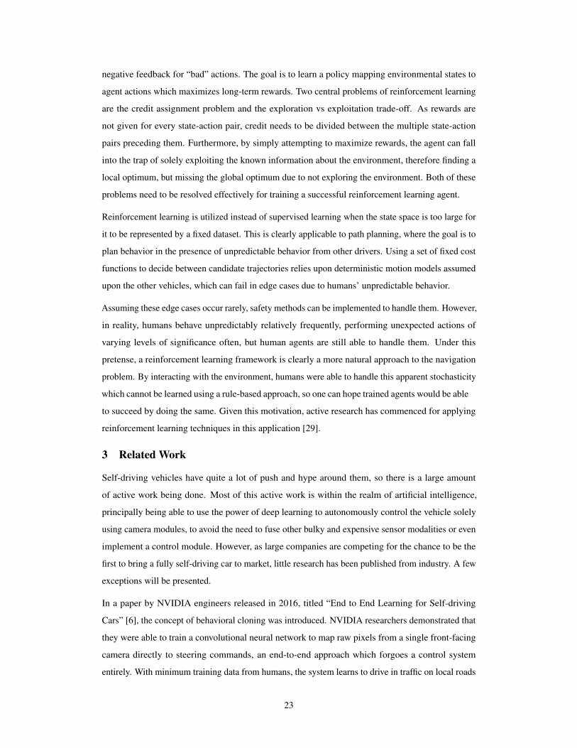
negative feedback for “bad” actions. The goal is to learn a policy mapping environmental states to
agent actions which maximizes long-term rewards. Two central problems of reinforcement learning
are the credit assignment problem and the exploration vs exploitation trade-off. As rewards are
not given for every state-action pair, credit needs to be divided between the multiple state-action
pairs preceding them. Furthermore, by simply attempting to maximize rewards, the agent can fall
into the trap of solely exploiting the known information about the environment, therefore finding a
local optimum, but missing the global optimum due to not exploring the environment. Both of these
problems need to be resolved effectively for training a successful reinforcement learning agent.
Reinforcement learning is utilized instead of supervised learning when the state space is too large for
it to be represented by a fixed dataset. This is clearly applicable to path planning, where the goal is to
plan behavior in the presence of unpredictable behavior from other drivers. Using a set of fixed cost
functions to decide between candidate trajectories relies upon deterministic motion models assumed
upon the other vehicles, which can fail in edge cases due to humans’ unpredictable behavior.
Assuming these edge cases occur rarely, safety methods can be implemented to handle them. However,
in reality, humans behave unpredictably relatively frequently, performing unexpected actions of
varying levels of significance often, but human agents are still able to handle them. Under this
pretense, a reinforcement learning framework is clearly a more natural approach to the navigation
problem. By interacting with the environment, humans were able to handle this apparent stochasticity
which cannot be learned using a rule-based approach, so one can hope trained agents would be able
to succeed by doing the same. Given this motivation, active research has commenced for applying
reinforcement learning techniques in this application [29].
3 Related Work
Self-driving vehicles have quite a lot of push and hype around them, so there is a large amount
of active work being done. Most of this active work is within the realm of artificial intelligence,
principally being able to use the power of deep learning to autonomously control the vehicle solely
using camera modules, to avoid the need to fuse other bulky and expensive sensor modalities or even
implement a control module. However, as large companies are competing for the chance to be the
first to bring a fully self-driving car to market, little research has been published from industry. A few
exceptions will be presented.
In a paper by NVIDIA engineers released in 2016, titled “End to End Learning for Self-driving
Cars” [6], the concept of behavioral cloning was introduced. NVIDIA researchers demonstrated that
they were able to train a convolutional neural network to map raw pixels from a single front-facing
camera directly to steering commands, an end-to-end approach which forgoes a control system
entirely. With minimum training data from humans, the system learns to drive in traffic on local roads
23

with or without lane markings and on highways. It also operates in areas with unclear visual guidance
such as in parking lots and on unpaved roads.
The system automatically learns internal representations of the necessary processing steps such as
detecting useful road features with only the human steering angle as the training signal. Compared to
explicit decomposition of the problem, such as lane marking detection, path planning, and control,
the end-to-end system optimizes all processing steps simultaneously. The researchers argue that
this will eventually lead to better performance and smaller systems. Better performance will result
because the internal components self-optimize to maximize overall system performance, instead of
optimizing human-selected intermediate criteria, e.g., lane detection. Such criteria understandably are
selected for ease of human interpretation which doesn’t automatically guarantee maximum system
performance. Smaller networks are possible because the system learns to solve the problem with the
minimal number of processing steps.
Figure 10: Training the neural network
The block diagram for their training system is shown in Figure 10. During training, three cameras
are mounted behind the windshield of the data-acquisition car, in order to have further variance
in the images to show the car in different shifts from the center of the lane and rotations from the
direction of the road. Once trained, the network can generate steering from the video images of a
single center camera. The final CNN architecture can be seen in Figure 11. The network has about 27
million connections and 250 thousand parameters. Evaluation was conducted both in simulation and
in on-road tests, where the vehicle succeeded in the situations presented to it [6].
Ford has also presented research in this field, albeit less ambitious than NVIDIA, focusing on lane
position estimation as opposed to behavioral cloning. An approach was presented to estimate lane
positions directly using a deep neural network that operates on images from laterally-mounted
down-facing cameras. Besides the ability to distinguish whether there is a lane-marker present or
not, the proposed network is able to estimate the position of a lane marker with sub-centimeter
accuracy at an average of 100 frames/s on an embedded automotive platform, requiring no pre- or
post-processing [15].
24
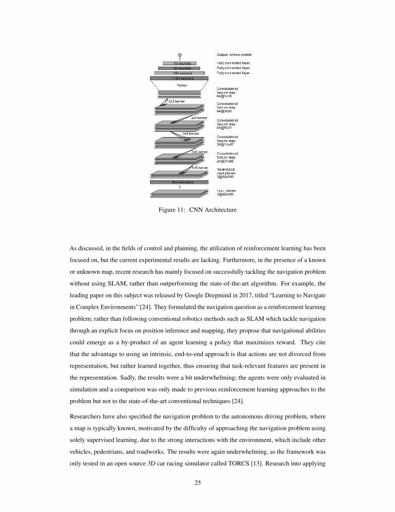
Figure 11: CNN Architecture
As discussed, in the fields of control and planning, the utilization of reinforcement learning has been
focused on, but the current experimental results are lacking. Furthermore, in the presence of a known
or unknown map, recent research has mainly focused on successfully tackling the navigation problem
without using SLAM, rather than outperforming the state-of-the-art algorithm. For example, the
leading paper on this subject was released by Google Deepmind in 2017, titled “Learning to Navigate
in Complex Environments” [24]. They formulated the navigation question as a reinforcement learning
problem; rather than following conventional robotics methods such as SLAM which tackle navigation
through an explicit focus on position inference and mapping, they propose that navigational abilities
could emerge as a by-product of an agent learning a policy that maximizes reward. They cite
that the advantage to using an intrinsic, end-to-end approach is that actions are not divorced from
representation, but rather learned together, thus ensuring that task-relevant features are present in
the representation. Sadly, the results were a bit underwhelming; the agents were only evaluated in
simulation and a comparison was only made to previous reinforcement learning approaches to the
problem but not to the state-of-the-art conventional techniques [24].
Researchers have also specified the navigation problem to the autonomous driving problem, where
a map is typically known, motivated by the difficulty of approaching the navigation problem using
solely supervised learning, due to the strong interactions with the environment, which include other
vehicles, pedestrians, and roadworks. The results were again underwhelming, as the framework was
only tested in an open source 3D car racing simulator called TORCS [13]. Research into applying
25
reinforcement learning for planning the navigation of self-driving cars is still in its early stages, but
preliminary signs indicate that this is a promising application of the science.
4 Project Description
The goal of our project is to build a system which enables a vehicle to navigate a model of a real-world
street map. The basis for such a system is lane keeping, the ability to stay within a lane. However,
real-world street maps are more than many lanes concatenated together; they incorporate intersections,
which is what a navigation system handles. We will describe the lane keeping and navigation systems,
as well as the software architecture, in this section.
4.1 Lane Keeping System
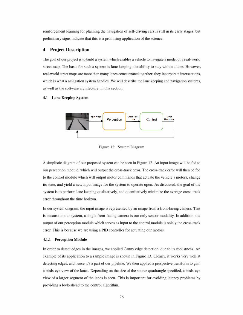
Figure 12: System Diagram
A simplistic diagram of our proposed system can be seen in Figure 12. An input image will be fed to
our perception module, which will output the cross-track error. The cross-track error will then be fed
to the control module which will output motor commands that actuate the vehicle’s motors, change
its state, and yield a new input image for the system to operate upon. As discussed, the goal of the
system is to perform lane keeping qualitatively, and quantitatively minimize the average cross-track
error throughout the time horizon.
In our system diagram, the input image is represented by an image from a front-facing camera. This
is because in our system, a single front-facing camera is our only sensor modality. In addition, the
output of our perception module which serves as input to the control module is solely the cross-track
error. This is because we are using a PID controller for actuating our motors.
4.1.1 Perception Module
In order to detect edges in the images, we applied Canny edge detection, due to its robustness. An
example of its application to a sample image is shown in Figure 13. Clearly, it works very well at
detecting edges, and hence it’s a part of our pipeline. We then applied a perspective transform to gain
a birds-eye view of the lanes. Depending on the size of the source quadrangle specified, a birds-eye
view of a larger segment of the lanes is seen. This is important for avoiding latency problems by
providing a look-ahead to the control algorithm.
26
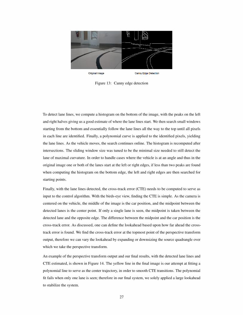
Figure 13: Canny edge detection
To detect lane lines, we compute a histogram on the bottom of the image, with the peaks on the left
and right halves giving us a good estimate of where the lane lines start. We then search small windows
starting from the bottom and essentially follow the lane lines all the way to the top until all pixels
in each line are identified. Finally, a polynomial curve is applied to the identified pixels, yielding
the lane lines. As the vehicle moves, the search continues online. The histogram is recomputed after
intersections. The sliding window size was tuned to be the minimal size needed to still detect the
lane of maximal curvature. In order to handle cases where the vehicle is at an angle and thus in the
original image one or both of the lanes start at the left or right edges, if less than two peaks are found
when computing the histogram on the bottom edge, the left and right edges are then searched for
starting points.
Finally, with the lane lines detected, the cross-track error (CTE) needs to be computed to serve as
input to the control algorithm. With the birds-eye view, finding the CTE is simple. As the camera is
centered on the vehicle, the middle of the image is the car position, and the midpoint between the
detected lanes is the center point. If only a single lane is seen, the midpoint is taken between the
detected lane and the opposite edge. The difference between the midpoint and the car position is the
cross-track error. As discussed, one can define the lookahead based upon how far ahead the cross-
track error is found. We find the cross-track error at the topmost point of the perspective transform
output, therefore we can vary the lookahead by expanding or downsizing the source quadrangle over
which we take the perspective transform.
An example of the perspective transform output and our final results, with the detected lane lines and
CTE estimated, is shown in Figure 14. The yellow line in the final image is our attempt at fitting a
polynomial line to serve as the center trajectory, in order to smooth CTE transitions. The polynomial
fit fails when only one lane is seen; therefore in our final system, we solely applied a large lookahead
to stabilize the system.
27
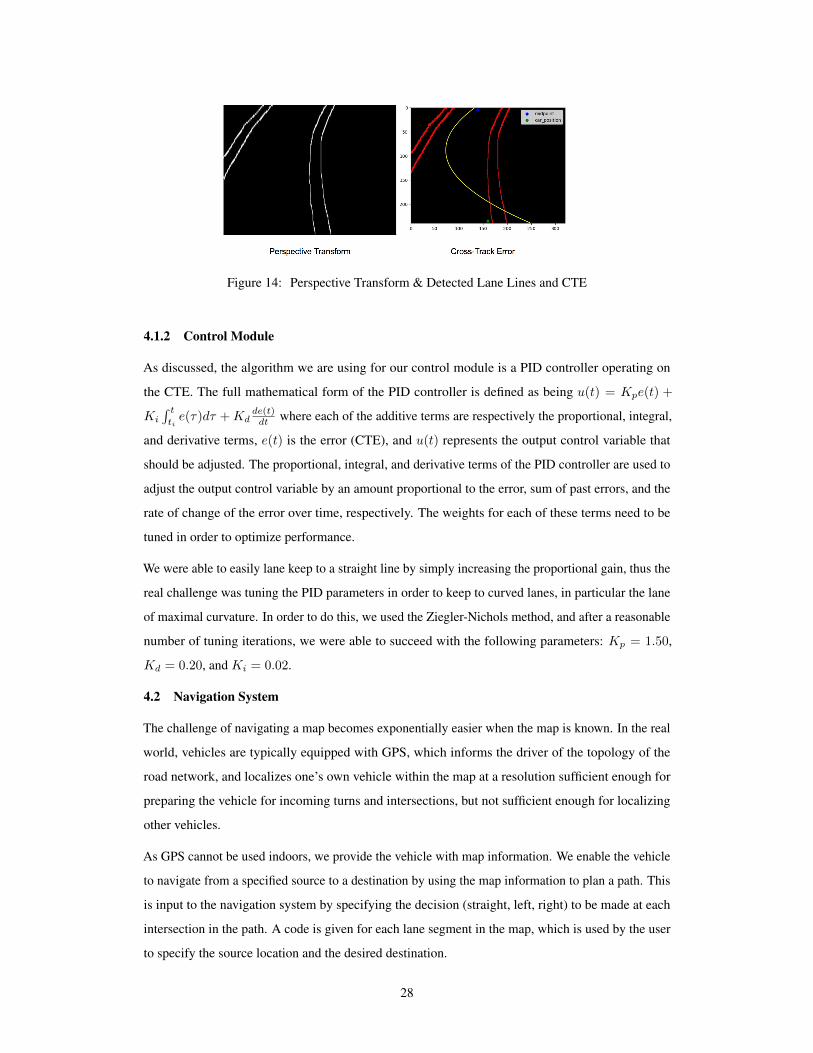
Figure 14: Perspective Transform & Detected Lane Lines and CTE
4.1.2 Control Module
As discussed, the algorithm we are using for our control module is a PID controller operating on
the CTE. The full mathematical form of the PID controller is defined as being u(t) = Kpe(t) +
Ki
∫ t
tie(τ)dτ +Kd
de(t)dt where each of the additive terms are respectively the proportional, integral,
and derivative terms, e(t) is the error (CTE), and u(t) represents the output control variable that
should be adjusted. The proportional, integral, and derivative terms of the PID controller are used to
adjust the output control variable by an amount proportional to the error, sum of past errors, and the
rate of change of the error over time, respectively. The weights for each of these terms need to be
tuned in order to optimize performance.
We were able to easily lane keep to a straight line by simply increasing the proportional gain, thus the
real challenge was tuning the PID parameters in order to keep to curved lanes, in particular the lane
of maximal curvature. In order to do this, we used the Ziegler-Nichols method, and after a reasonable
number of tuning iterations, we were able to succeed with the following parameters: Kp = 1.50,
Kd = 0.20, and Ki = 0.02.
4.2 Navigation System
The challenge of navigating a map becomes exponentially easier when the map is known. In the real
world, vehicles are typically equipped with GPS, which informs the driver of the topology of the
road network, and localizes one’s own vehicle within the map at a resolution sufficient enough for
preparing the vehicle for incoming turns and intersections, but not sufficient enough for localizing
other vehicles.
As GPS cannot be used indoors, we provide the vehicle with map information. We enable the vehicle
to navigate from a specified source to a destination by using the map information to plan a path. This
is input to the navigation system by specifying the decision (straight, left, right) to be made at each
intersection in the path. A code is given for each lane segment in the map, which is used by the user
to specify the source location and the desired destination.
28
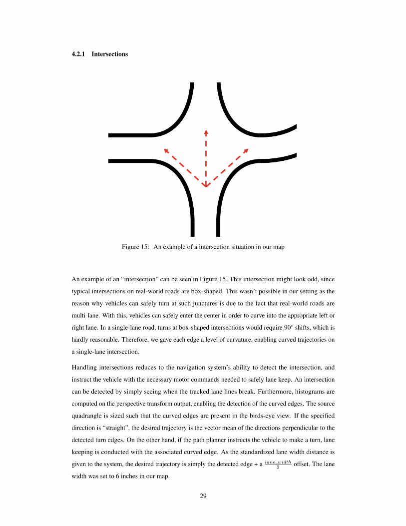
4.2.1 Intersections
Figure 15: An example of a intersection situation in our map
An example of an “intersection” can be seen in Figure 15. This intersection might look odd, since
typical intersections on real-world roads are box-shaped. This wasn’t possible in our setting as the
reason why vehicles can safely turn at such junctures is due to the fact that real-world roads are
multi-lane. With this, vehicles can safely enter the center in order to curve into the appropriate left or
right lane. In a single-lane road, turns at box-shaped intersections would require 90° shifts, which is
hardly reasonable. Therefore, we gave each edge a level of curvature, enabling curved trajectories on
a single-lane intersection.
Handling intersections reduces to the navigation system’s ability to detect the intersection, and
instruct the vehicle with the necessary motor commands needed to safely lane keep. An intersection
can be detected by simply seeing when the tracked lane lines break. Furthermore, histograms are
computed on the perspective transform output, enabling the detection of the curved edges. The source
quadrangle is sized such that the curved edges are present in the birds-eye view. If the specified
direction is “straight”, the desired trajectory is the vector mean of the directions perpendicular to the
detected turn edges. On the other hand, if the path planner instructs the vehicle to make a turn, lane
keeping is conducted with the associated curved edge. As the standardized lane width distance is
given to the system, the desired trajectory is simply the detected edge + a lane_width2 offset. The lane
width was set to 6 inches in our map.
29
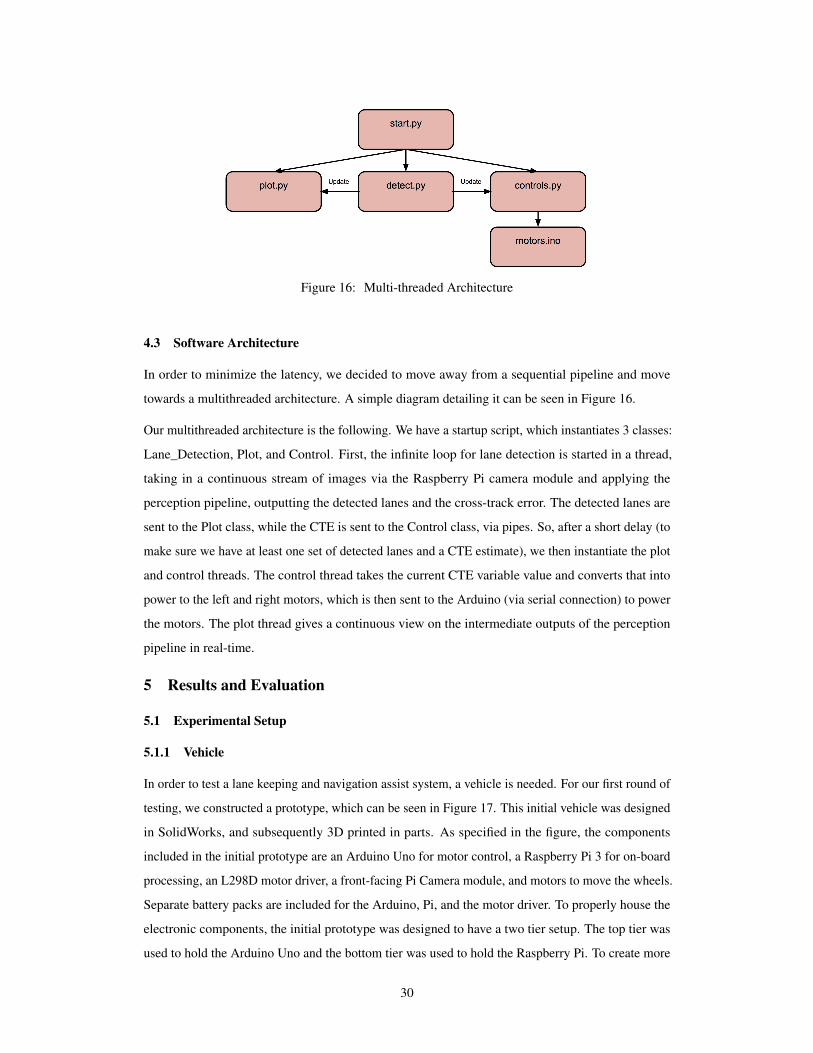
Figure 16: Multi-threaded Architecture
4.3 Software Architecture
In order to minimize the latency, we decided to move away from a sequential pipeline and move
towards a multithreaded architecture. A simple diagram detailing it can be seen in Figure 16.
Our multithreaded architecture is the following. We have a startup script, which instantiates 3 classes:
Lane_Detection, Plot, and Control. First, the infinite loop for lane detection is started in a thread,
taking in a continuous stream of images via the Raspberry Pi camera module and applying the
perception pipeline, outputting the detected lanes and the cross-track error. The detected lanes are
sent to the Plot class, while the CTE is sent to the Control class, via pipes. So, after a short delay (to
make sure we have at least one set of detected lanes and a CTE estimate), we then instantiate the plot
and control threads. The control thread takes the current CTE variable value and converts that into
power to the left and right motors, which is then sent to the Arduino (via serial connection) to power
the motors. The plot thread gives a continuous view on the intermediate outputs of the perception
pipeline in real-time.
5 Results and Evaluation
5.1 Experimental Setup
5.1.1 Vehicle
In order to test a lane keeping and navigation assist system, a vehicle is needed. For our first round of
testing, we constructed a prototype, which can be seen in Figure 17. This initial vehicle was designed
in SolidWorks, and subsequently 3D printed in parts. As specified in the figure, the components
included in the initial prototype are an Arduino Uno for motor control, a Raspberry Pi 3 for on-board
processing, an L298D motor driver, a front-facing Pi Camera module, and motors to move the wheels.
Separate battery packs are included for the Arduino, Pi, and the motor driver. To properly house the
electronic components, the initial prototype was designed to have a two tier setup. The top tier was
used to hold the Arduino Uno and the bottom tier was used to hold the Raspberry Pi. To create more
30
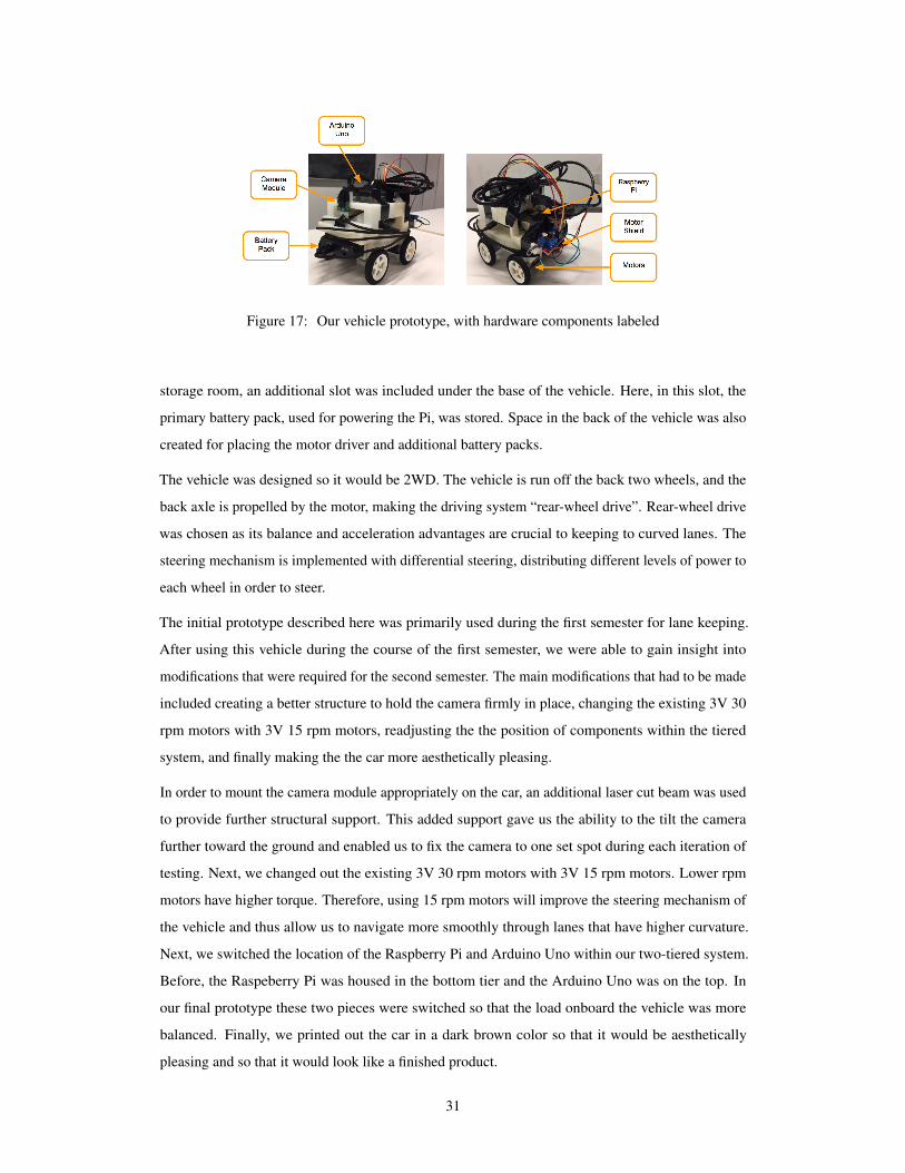
Figure 17: Our vehicle prototype, with hardware components labeled
storage room, an additional slot was included under the base of the vehicle. Here, in this slot, the
primary battery pack, used for powering the Pi, was stored. Space in the back of the vehicle was also
created for placing the motor driver and additional battery packs.
The vehicle was designed so it would be 2WD. The vehicle is run off the back two wheels, and the
back axle is propelled by the motor, making the driving system “rear-wheel drive”. Rear-wheel drive
was chosen as its balance and acceleration advantages are crucial to keeping to curved lanes. The
steering mechanism is implemented with differential steering, distributing different levels of power to
each wheel in order to steer.
The initial prototype described here was primarily used during the first semester for lane keeping.
After using this vehicle during the course of the first semester, we were able to gain insight into
modifications that were required for the second semester. The main modifications that had to be made
included creating a better structure to hold the camera firmly in place, changing the existing 3V 30
rpm motors with 3V 15 rpm motors, readjusting the the position of components within the tiered
system, and finally making the the car more aesthetically pleasing.
In order to mount the camera module appropriately on the car, an additional laser cut beam was used
to provide further structural support. This added support gave us the ability to the tilt the camera
further toward the ground and enabled us to fix the camera to one set spot during each iteration of
testing. Next, we changed out the existing 3V 30 rpm motors with 3V 15 rpm motors. Lower rpm
motors have higher torque. Therefore, using 15 rpm motors will improve the steering mechanism of
the vehicle and thus allow us to navigate more smoothly through lanes that have higher curvature.
Next, we switched the location of the Raspberry Pi and Arduino Uno within our two-tiered system.
Before, the Raspeberry Pi was housed in the bottom tier and the Arduino Uno was on the top. In
our final prototype these two pieces were switched so that the load onboard the vehicle was more
balanced. Finally, we printed out the car in a dark brown color so that it would be aesthetically
pleasing and so that it would look like a finished product.
31
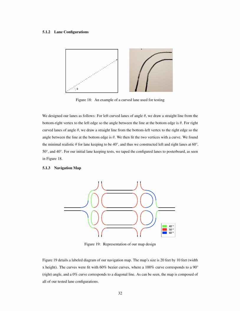
5.1.2 Lane Configurations
Figure 18: An example of a curved lane used for testing
We designed our lanes as follows: For left curved lanes of angle θ, we draw a straight line from the
bottom-right vertex to the left edge so the angle between the line at the bottom edge is θ. For right
curved lanes of angle θ, we draw a straight line from the bottom-left vertex to the right edge so the
angle between the line at the bottom edge is θ. We then fit the two vertices with a curve. We found
the minimal realistic θ for lane keeping to be 40°, and thus we constructed left and right lanes at 60°,
50°, and 40°. For our initial lane keeping tests, we taped the configured lanes to posterboard, as seen
in Figure 18.
5.1.3 Navigation Map
Figure 19: Representation of our map design
Figure 19 details a labeled diagram of our navigation map. The map’s size is 20 feet by 10 feet (width
x height). The curves were fit with 60% bezier curves, where a 100% curve corresponds to a 90°
(right) angle, and a 0% curve corresponds to a diagonal line. As can be seen, the map is composed of
all of our tested lane configurations.
32
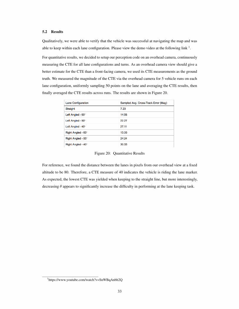
5.2 Results
Qualitatively, we were able to verify that the vehicle was successful at navigating the map and was
able to keep within each lane configuration. Please view the demo video at the following link 1.
For quantitative results, we decided to setup our perception code on an overhead camera, continuously
measuring the CTE for all lane configurations and turns. As an overhead camera view should give a
better estimate for the CTE than a front-facing camera, we used its CTE measurements as the ground
truth. We measured the magnitude of the CTE via the overhead camera for 5 vehicle runs on each
lane configuration, uniformly sampling 50 points on the lane and averaging the CTE results, then
finally averaged the CTE results across runs. The results are shown in Figure 20.
Figure 20: Quantitative Results
For reference, we found the distance between the lanes in pixels from our overhead view at a fixed
altitude to be 80. Therefore, a CTE measure of 40 indicates the vehicle is riding the lane marker.
As expected, the lowest CTE was yielded when keeping to the straight line, but more interestingly,
decreasing θ appears to significantly increase the difficulty in performing at the lane keeping task.
1https://www.youtube.com/watch?v=SnWBqAnbh2Q
33
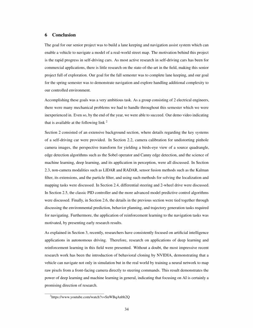
6 Conclusion
The goal for our senior project was to build a lane keeping and navigation assist system which can
enable a vehicle to navigate a model of a real-world street map. The motivation behind this project
is the rapid progress in self-driving cars. As most active research in self-driving cars has been for
commercial applications, there is little research on the state-of-the-art in the field, making this senior
project full of exploration. Our goal for the fall semester was to complete lane keeping, and our goal
for the spring semester was to demonstrate navigation and explore handling additional complexity to
our controlled environment.
Accomplishing these goals was a very ambitious task. As a group consisting of 2 electrical engineers,
there were many mechanical problems we had to handle throughout this semester which we were
inexperienced in. Even so, by the end of the year, we were able to succeed. Our demo video indicating
that is available at the following link 2
Section 2 consisted of an extensive background section, where details regarding the key systems
of a self-driving car were provided. In Section 2.2, camera calibration for undistorting pinhole
camera images, the perspective transform for yielding a birds-eye view of a source quadrangle,
edge detection algorithms such as the Sobel operator and Canny edge detection, and the science of
machine learning, deep learning, and its application in perception, were all discussed. In Section
2.3, non-camera modalities such as LIDAR and RADAR, sensor fusion methods such as the Kalman
filter, its extensions, and the particle filter, and using such methods for solving the localization and
mapping tasks were discussed. In Section 2.4, differential steering and 2-wheel drive were discussed.
In Section 2.5, the classic PID controller and the more advanced model predictive control algorithms
were discussed. Finally, in Section 2.6, the details in the previous section were tied together through
discussing the environmental prediction, behavior planning, and trajectory generation tasks required
for navigating. Furthermore, the application of reinforcement learning to the navigation tasks was
motivated, by presenting early research results.
As explained in Section 3, recently, researchers have consistently focused on artificial intelligence
applications in autonomous driving. Therefore, research on applications of deep learning and
reinforcement learning in this field were presented. Without a doubt, the most impressive recent
research work has been the introduction of behavioral cloning by NVIDIA, demonstrating that a
vehicle can navigate not only in simulation but in the real world by training a neural network to map
raw pixels from a front-facing camera directly to steering commands. This result demonstrates the
power of deep learning and machine learning in general, indicating that focusing on AI is certainly a
promising direction of research.
2https://www.youtube.com/watch?v=SnWBqAnbh2Q
34

In Section 4, our lane keeping system, navigation system, and software architecture were presented.
Our lane keeping system is composed of perception and control modules interacting with the vehicle
in a feedback loop. The following cycle continuously takes place: the front-facing camera takes an
image, the perception module yields the cross-track error, and the control module yields the motor
commands which would propel the vehicle forward. The perception module consists of detecting the
edges in the image, acquiring a birds-eye view of the lanes, detecting the lane lines with a sliding
window approach, and computing the error between the car position and the midpoint between the
lanes. The PID controller is tuned to minimize that error. For navigation, map information is provided
to the system to allow a path to be planned between a specified source and destination. Turns are
handled by appropriately lane keeping to the intersection’s curved edge, which is required due to the
single-lane nature of our map. To minimize latency, the described systems have been implemented in
a multithreaded software architecture.
In Section 5, we detailed our experimental setup and our qualitative and quantitative results. In
order to experiment, we built a test vehicle and printed out a map consisting of lane configurations
with varying levels of curvature, where the curvature was tuned with the θ parameter. Qualitatively,
we verified that the vehicle was capable of navigating the map while staying within the lane lines,
while our quantitative results indicate that increasing the curvature scales up the difficulty of the lane
keeping task considerably.
We believe adding real-world complexities to our controlled environment, and enabling the system to
navigate under environmental noise and with dynamic obstacles (other vehicles) present, is certainly
a valuable direction for future work. We were able to verify in our experiments that the system can
handle mild noise. For example, placing receipts and brown napkins on the curved lanes, which
contrast with the background, doesn’t cause the vehicle to falter. However, adding true real-world
noise to the physical environment can only be done by transitioning to the real world, which isn’t
possible for our miniature vehicle which has been tuned to handle a single-lane map. Furthermore,
adding dynamic obstacles, such as other vehicles, would involve building other vehicles and expanding
the map to consist of two-lane roads. In short, handling these complexities added not in simulation
but to the physical experimental setup is nontrivial, but taking this next step would bring this system
one step further to becoming a true real-world self-driving car system.
35

References
[1] 2wd vs awd vs 4wd:a guide to the differences and which is best for you.
https://www.consumerreports.org/cro/2012/12/2wd-awd-or-4wd-how-much-traction-do-
you-need/index.htm.
[2] Advanced lane detection. https://medium.com/@MSqalli/advanced-lane-detection-
6a769de0d581.
[3] Introduction: Pid controller design. http://ctms.engin.umich.edu/CTMS/index.php?example=Introductionsection=ControlPID.
[4] Lane detection with deep learning (part 1). https://towardsdatascience.com/lane-detection-with-
deep-learning-part-1-9e096f3320b7.
[5] A short history of color edge detection. http://ai.stanford.edu/ ruzon/compass/color.html.
[6] M. Bojarski, D. Del Testa, D. Dworakowsi, B. Firner, B. Flepp, P. Goyal, L.D. Jackel, M. Mon-
fort, U. Muller, and J. Zhang. End-to-end learning for self-driving cars. 2016.
[7] John Canny. A computational approach to edge detection. IEEE Transactions on Pattern
Analysis And Machine Intelligence, 1986.
[8] Navneet Dalal and Bill Triggs. Histograms of oriented gradients for human detection. In
Proceedings of the 2005 IEEE Computer Society Conference on Computer Vision and Pattern
Recognition (CVPR’05) - Volume 1 - Volume 01, CVPR ’05, pages 886–893, Washington, DC,
USA, 2005. IEEE Computer Society.
[9] P. Del Moral. Non-linear filtering: Interacting particle solution. 1996.
[10] J. Deng, W. Dong, R. Socher, L.J. Li, K. Li, and Fei-Fei Li. Imagenet: A large-scale hierarchical
image database. 2009.
[11] G. Dissanayake, P. Newman, S. Clark, H. Durrant-Whyte, and M. Csorba. A solution to the
simultaneous localization and map building problem. 2001.
[12] Gregory Dudek and Michael Jenkin. Computational principles of mobile robotics. 2010.
[13] A. El Sallab, M. Abdou, E. Perot, and S. Yogamani. Deep reinforcement learning framework
for autonomous driving. 2017.
[14] Ian Goodfellow, Yoshua Bengio, and Aaron Courville. Deep learning. 2016.
[15] Alexandru Gurghian, Tejaswi Koduri, Smita Bailur, Kyle Carey, and Vidya Murali. DeepLanes:
End-To-End Lane Position Estimation using Deep Neural Networks. 2016.
36
[16] Aharon Bar Hillel, Ronen Lerner, Dan Levi, and Guy Raz. Recent Progress in Road and Lane
Detection - A survey. 2014.
[17] N. Hogan. Adaptive control of mechanical impedance by coactivation of antagonist muscles.
1984.
[18] S.J. Julier and J.K. Uhlmann. A new extension of the kalman filter to nonlinear systems. 1997.
[19] R.E. Kalman. A new approach to linear filtering and prediction problems. 1960.
[20] Nick Kanopoulos and et.al. Design of an image edge detection filter using the sobel operator.
Journal of Solid State Circuits, pages 358–367, 1988.
[21] A. Krizhevsky, I. Sutskever, and G. Hinton. Imagenet classification with deep convolutional
neural networks. 2012.
[22] Yann LeCun, Léon Bottou, Yoshua Bengio, and Patrick Haffner. Gradient-based learning
applied to document recognition. In Proceedings of the IEEE, volume 86, pages 2278–2324,
1998.
[23] Q. Li, N. Zheng, and H. Cheng. A prototype autonomous vehicle and its algorithms for lane
detection. IEEE Trans. Intell. Transp.Systems, pages 300–308, 2004.
[24] P. Mirowski, R. Pascanu, F. Viola, H. Soyer, A. Ballard, A. Banino, M. Denil, R. Goroshin,
L. Sifre, K. Kavukcuoglu, D. Kumaran, and R. Hadsell. Learning to navigate in complex
environments. 2017.
[25] M. Montemerlo, J. Becker, S. Bhat, H. Dahlkamp, D. Dolgov, S. Ettinger, D. Haehnel, T. Hilden,
G. Hoffmann, B. Huhnke, D. Johnston, S. Klumpp, D. Langer, A. Levandowski, J. Levinson,
J. Marcil, D. Orenstein, J. Paefgen, I. Penny, A. Petrovskaya, M. Pflueger, G. Stanek, D. Stavens,
A. Vogt, and S. Thrun. Junior: The stanford entry in the urban challenge. 2008.
[26] H. Nyquist. Regeneration theory. 1932.
[27] Daniel Oliva Sales, Leandro Fernandes, Fernando Osorio, and Denis Wolf. Fsm-based visual
navigation for autonomous vehicles, 10 2012.
[28] R. Schubert, E. Richter, and G. Wanielik. Comparison and evaluation of advanced motion
models for vehicle tracking. 2008.
[29] R. Sutton and A. Barto. Reinforcement learning: An introduction. 1998.
[30] R. Szeliski. Computer vision: Algorithms and applications. 2010.
37
[31] S. Thrun, M. Montemerlo, H. Dahlkamp, D. Stavens, A. Aron, J. Diebel, P. Fong, J. Gale,
M. Halpenny, G. Hoffmann, K. Lau, C. Oakley, M. Palatucci, V. Pratt, P. Stang, S. Strohband,
C. Dupont, L.E. Jendrossek, C. Koelen, C. Markey, C. Rummel, J. van Niekerk, E. Jensen,
P. Alessandrini, G. Bradski, B. Davies, S. Ettinger, A. Kaehler, A. Nefian, and P. Mahoney.
Stanley: The robot that won the darpa grand challenge. 2006.
[32] C. Urmson, J. Anhalt, D. Bagnell, C. Baker, R. Bittner, M.N. Clark, J. Dolan, D. Duggins,
T. Galatali, C. Geyer, M. Gittleman, S. Harbaugh, M. Hebert, T.M. Howard, S. Kolski, A. Kelly,
M. Likhachev, M. McNaughton, N. Miller, K. Peterson, B. Pilnick, R. Rajkumar, P. Rybski,
B. Salesky, Y.-W. Seo, S. Singh, J. Snider, A. Stentz, W. Whittaker, Z. Wolkowicki, J. Ziglar,
H. Bae, T. Brown, D. Demitrish, B. Litkouhi, J. Nickolaou, V. Sadekar, W. Zhang, Taylor M.
Struble, J., M. Darms, and D. Ferguson. Autonomous driving in urban environments: Boss and
the urban challenge. 2008.
[33] L. Wang. Model predictive control system design and implementation. 2009.
[34] D. Wolpert. The lack of a priori distinctions between learning algorithms. 1996.
[35] Z. Zhang. A flexible new technique for camera calibration. 2000.
[36] J.G. Ziegler and N.B. Nichols. Optimum settings for automatic controllers. 1942.
38