The Munich Re Programme: Evaluating the Economics

of Climate Risks and Opportunities in the Insurance Sector

Laplace’s Demon and Climate Change

Roman Frigg, Seamus Bradley, Hailiang Du and Leonard A. Smith

January 2013

Centre for Climate Change Economics and Policy Working Paper No. 121

Munich Re Programme Technical Paper No. 17

Grantham Research Institute on Climate Change and the Environment

Working Paper No. 103

The Centre for Climate Change Economics and Policy (CCCEP) was established by the University of Leeds and the London School of Economics and Political Science in 2008 to advance public and private action on climate change through innovative, rigorous research. The Centre is funded by the UK Economic and Social Research Council and has five inter-linked research programmes:

1. Developing climate science and economics 2. Climate change governance for a new global deal 3. Adaptation to climate change and human development 4. Governments, markets and climate change mitigation 5. The Munich Re Programme - Evaluating the economics of climate risks and

opportunities in the insurance sector (funded by Munich Re) More information about the Centre for Climate Change Economics and Policy can be found at: http://www.cccep.ac.uk. The Munich Re Programme is evaluating the economics of climate risks and opportunities in the insurance sector. It is a comprehensive research programme that focuses on the assessment of the risks from climate change and on the appropriate responses, to inform decision-making in the private and public sectors. The programme is exploring, from a risk management perspective, the implications of climate change across the world, in terms of both physical impacts and regulatory responses. The programme draws on both science and economics, particularly in interpreting and applying climate and impact information in decision-making for both the short and long term. The programme is also identifying and developing approaches that enable the financial services industries to support effectively climate change adaptation and mitigation, through for example, providing catastrophe insurance against extreme weather events and innovative financial products for carbon markets. This programme is funded by Munich Re and benefits from research collaborations across the industry and public sectors. The Grantham Research Institute on Climate Change a nd the Environment was established by the London School of Economics and Political Science in 2008 to bring together international expertise on economics, finance, geography, the environment, international development and political economy to create a world-leading centre for policy-relevant research and training in climate change and the environment. The Institute is funded by the Grantham Foundation for the Protection of the Environment and the Global Green Growth Institute, and has five research programmes:

1. Global response strategies 2. Green growth 3. Practical aspects of climate policy 4. Adaptation and development 5. Resource security

More information about the Grantham Research Institute on Climate Change and the Environment can be found at: http://www.lse.ac.uk/grantham. This working paper is intended to stimulate discussion within the research community and among users of research, and its content may have been submitted for publication in academic journals. It has been reviewed by at least one internal referee before publication. The views expressed in this paper represent those of the author(s) and do not necessarily represent those of the host institutions or funders.

1

Laplace’s Demon and Climate Change

Roman Frigg, Seamus Bradley, Hailiang Du and Leonard A. Smith1

1. Introduction: Laplace’s Demon

Knowing what the future will bring is an age-old human desire. Yet it is a desire

mortals find difficult to satisfy, and creatures endowed with appropriate powers tend

to inhabit fictional landscapes. Among those creatures Laplace’s Demon has gained

notoriety. Laplace (1814, 4) invites us to consider a supreme intelligence who is able

to identify all basic components of nature and the forces acting between them, and

then observe these components’ initial conditions. On the basis of this information the

Demon knows the deterministic equations of motion of the world and uses his

supreme computational power to solve them. The solutions of the equations of motion

together with the initial conditions tell him everything he wants to know so that

‘nothing would be uncertain and the future, as the past, would be present to [his] eyes’

(ibid.). This operationally omniscient creature is now known as Laplace’s Demon.

Let us give precise statement of the Demon’s capabilities. In order to predict the

future, the Demon possesses a mathematical model of the world. It is part of

Laplace’s original scenario that the model is a model of the entire world. However,

nothing in what follows depends on the model being global in this sense, and so we

consider a scenario in which the Demon’s predicts the behaviour of a particular part

or aspect of the world (which can but need not be the entire world). In line with much

of the literature on modelling we refer to this part or aspect of the world as the target

system. Mathematically modelling a target system amounts to introducing a

dynamical system ),,( µφtX , which represents that target system.2 Unlike the target

1 To contact the authors write to r.p.frigg@lse.ac.uk; s.c.bradley@lse.ac.uk; h.l.du@lse.ac.uk and

lenny@maths.ox.ac.uk. 2 Calling both the model and the target ‘system’ is unfortunate; we do so only in order to stick with

conventionally used terminology. For a discussion of the anatomy of scientific modelling can be found

in (Frigg 2010).

2

system, which is part of the material world, a dynamical system is a mathematical

object. As indicated by the notation, a dynamical system consists of three elements.

The first element, X , is the system’s state space. When we take ),,( µφtX to

represent a target system, the states in X are taken to represent states of the target

system. For instance, the state space of a particle moving along a line consists of all

tuples ),( pqx = , where q and p are real numbers representing, respectively, the

particle’s position and momentum. The second element, tφ , is the time evolution: if

the system is in state Xx ∈0 at time 0=t , then it is in )( 0xy tφ= at some later time

t ; that is, tφ tells us how the system’s state changes in time. The state 0x is called the

system’s initial condition. Often tφ for a particular system is not formulated directly;

instead we formulate the system’s equation of motion and then tφ is the solution of

that equation. In the dynamical systems we are concerned with in this paper, the time

evolution of a system is generated by the repeated application of a map U at discrete

time steps: tt U=φ , for ,...2,1,0=t 3 The third element, µ , is the system’s Lebesgue

measure: it allows us to say that parts of X have certain size. In case X is the real

axis, µ is the length of an interval. The measure is used both to measure physical

distance, and (as we will see) it plays a role in defining a probability density over X .

With this bit of formal apparatus in place, we can describe Laplace’s Demon as a

creature with the following capabilities:

(1) He has unlimited computational power: he is able to calculate

instantaneously )(xy tφ= for all t and for any x .

(2) He has unlimited observational power: he is able to specify the true initial

condition 0x .

(3) He has unlimited dynamical knowledge: he is able to formulate the true

time evolution tφ .

3 This is a common assumption. For an introduction to dynamical systems see (Arnold and Avez 1968).

3

If these conditions are met, it is indeed the case that ‘nothing would be uncertain’ to

the Demon and ‘the future, as the past, would be present to [his] eyes’.4 In the

modelling literature having the true tφ is often referred to as the Perfect Model

Scenario; so condition (3) says that the Demon has the perfect (or true) model.

Humans do not have any of the Demon’s capabilities: most equations we can’t solve,

no measurement can ever reveal an exact initial condition, and for most systems

idealisations are unavoidable when formulating equations. It is therefore no surprise

that Laplace was quick to point out that the human mind ‘will always remain

infinitely removed’ from the Demon’s intelligence, of which it offers only a ‘feeble

idea’ (ibid.). The interesting question in connection with Laplace’s Demon is not

whether we fail to perform at the Demon’s level – of course we do. The interesting

question is how exactly we fail and what the consequences of this failure are.

Laplace’s own discussion emphasises the Demon’s unlimited computational power

and sees our main failure in being unable to do the calculations that the demon is able

to do. This was indicative of the concerns of physicists and mathematicians at the

time, when the focus was on developing techniques to solve differential equations.

Interestingly, Laplace paid little attention to the other two conditions.5 It is difficult to

say in retrospect what exactly his and his contemporaries’ attitude towards conditions

(2) and (3) was, but given that only scant attention was paid to them, it cannot be far

off the mark to assume that they were considered practical limitations of little

theoretical interest.

The old view that the unavailability of exact initial conditions is no impediment to

making successful predictions in a deterministic system was based on what is now

known as the strong principle of causality. The principle says that if y0, the initial

condition used for calculations, is close enough to x0, the true initial condition, then 4 Laplace implies that the dynamics is invertible. We ignore cases in which this is not the case because

we restrict attention on prediction. 5 He briefly mentions that the Demon must ‘comprehend all the forces by which nature is animated and

respective situation of beings who compose it’ (1814, 4). It is reasonable to assume that Laplace had

the true forces (and hence the true equation of motion) and the true initial positions in mind, but he

does not dwell on the point.

4

the trajectories originating in x0 and y0 stay together for all times – varying the initial

conditions a little bit will not change the outcome very much. When confronted with

the task of making a prediction, we have to assess what the required precision is and

then make a sufficiently precise measurement of the initial condition. This may be

challenging in practice, but in essence it is an engineering problem of no in-principle

importance.

This way of thinking about initial conditions was debunked by Poincaré at the

beginning of the last century. Poincaré’s crucial insight was that if a system’s

dynamics is non-linear (and most systems are better modelled as non-linear), then

even arbitrarily close initial conditions can diverge and end up taking very different

paths – an effect now known as sensitive dependence on initial conditions.6 So we

cannot infer from the fact that initial conditions are similar that the later trajectories

will be similar too. But if arbitrarily small variations in the initial condition can make

a dramatic difference, then the strong principle of causality is wrong and we can no

longer dismiss issues surrounding initial conditions a merely practical problem. In

fact, the failure of the strong principle has wide-ranging consequences, and the study

of these consequences is known as the study of chaos. So condition (2) is much less

innocuous than it originally seemed to be.

Similar issues arise in connection with condition (3). Just as we cannot get our hands

on the true initial condition, we cannot formulate the true equations of motion of a

target system (if such equations exist at all). Idealisations, distortions, omissions and

simplifications are inevitable. We model oblate spheroid planets as perfect spheres,

sticky surfaces as frictionless, markets as having no transaction costs, and so on. This

has of course long been recognised, but, as with condition (2), dismissed as a practical

issue of no in-principle importance. However, this dismissal has rarely, if ever, been

explicit. A tacit consensus has emerged that we are entitled to assume that if the

equations of our model are close enough to the true equations, then the predictions the

model makes are close enough. We call this assumption the closeness-to-goodness

6 This is effect is often referred to as chaos, but in fact the relation between sensitive dependence and

chaos is not straightforward; for a discussion of this point see (Smith 1998, Ch. 10).

5

link. This link is the ‘model-level analogue’ of the strong principle of causality – the

reasoning behind both principles is that close enough is good enough.

Unlike the strong principle of causality, the closeness-to-goodness link has not yet

attracted much attention. The central contention of this paper is that closeness-to-

goodness link does not fare better then the strong principle of causality: even the

slightest inaccuracy in the specification of the system’s dynamics destroys the

Demon’s ability to predict the future. More specifically we argue that if a

mathematical model is non-linear and if there is only a minuscule structural model

imperfection, then treating model outputs as decision-relevant forecasts can be

seriously misleading: the closeness-to-goodness link fails. And the worst is yet to

come: this is the case even if we were to limit attention to making probabilistic

forecasts. Unless the Demon has the true equations of motion, he cannot even make

reliable probabilistic forecasts.

This is more than a pedantic addition to a contrived thought experiment. In fact, this

addition has important implication for scientific practice because understanding the

conditions that need to be met by the Demon to make reliable predictions teaches us

important lessons about our own limitations. From planetary motion to nuclear

fission, from inventory control to sea level rise, and from the growth of populations to

the returns of an investment, and from short term weather forecasts to long term

climate predictions, there is hardly a phenomenon that has not at one point or other

been modelled mathematically, and the mathematical models are often used for the

purpose of forecasting. Moreover, there is a general trend, aided by the availability of

ever increasing computational power, of building ever larger and more complex

mathematical models of an ever growing variety of systems. This trend is particularly

prevalent in both climate science and in weather forecasting, where ever larger

models are constructed and run with the aim of making specific predictions.

This raises the question of exactly what man-made models deliver: can they provide

the results as advertised? This is where Laplace’s Demon comes into play. The limits

of the Demon are at once the limits of every mathematical modelling endeavour: the

fact that the Demon loses his predictive powers if there is only a small inaccuracy in

6

this specification of the system’s dynamics has profound implications for what we can

and cannot do with our mathematical models.

In Section 2 we introduce the Demon’s freshman apprentice, who shares some but not

all capabilities of the Demon. In Section 3 we let the apprentice offer bets in a

concrete situation based on the logistic map, and document his failures. This shows in

an exemplary manner what can go wrong if probabilities are used naively in an

imperfect model scenario. While one counterexample is sufficient to refute a general

view, it is important that the example used is not idiosyncratic and easily dismissed as

being irrelevant to those cases we really care about. This question is addressed in

Section 4, where we provide a general mathematical argument for the conclusion the

problems described in Section 3 are generic and occur in a large class of systems. In

Section 5 we discuss some concrete cases where the methodologies we criticise are

used; most notably climate and weather models belong to this class. In Section 6 we

discuss and dismiss a number of simple ways around the problem and in Section 7 we

present our own tentative solution, which suggests abandoning probabilism and using

non-probability odds instead. In Section 8 we draw some general conclusions.

2. Probabilistic Forecasting: The Demon’s Apprentice

It is now time to meet the Demon’s apprentices – the freshman apprentice and the

advanced apprentice. Like the master, both apprentices can calculate )(xy tφ=

instantaneously for all t and for any x . The senior apprentice also shares with the

Demon the ability to know the true time evolution operator tφ , but has limited

observational power and can specify the system’s initial condition only with a certain

margin of error (or, as physicists, would say: he only has noisy observations).7 The

freshman apprentice yet has to acquire the skills of the senior apprentice and can

neither specify a precise initial condition nor know the true time evolution.

7 This is the apprentice we have already encountered in (Smith 2007).

7

Both apprentices are aware of their limitations and come up with coping mechanisms.

In order to overcome the limited knowledge about initial conditions, when making

calculations, they both account for their uncertainty by considering a probability

distribution )(0 xp over relevant initial states, where the subscript indicates that the

distribution describes their uncertainty about the initial condition at 0=t .8 For the

apprentices, therefore, it makes no sense to move a single precise initial condition

forward in time; for them the relevant question is how initial probabilities change over

the course of time. To answer this question they use tφ to move )(0 xp forward in

time; that is, they calculate )]([:)( 0 xpxp tt φ= .9

This idea is simple and striking: if )(0 xp provides them with the probability of

finding the system’s state at a particular place in X at 0=t , then )(xpt is the

probability of finding the system’s state at a particular place at any later time t . We

call the apprentices’ view that decision-relevant probabilities for certain events to

occur can be obtained by using tφ to obtain forecast probabilities for events at later

times the default position. The qualification ‘decision-relevant’ is crucial. The Default

Position does not make the (trivial) statement that )(xpt is a probability distribution in

a purely formal sense of being an object that satisfies the mathematical axioms of

probability; the position is committed to the (non-trivial) claim that these probabilities

are the true probabilities for outcomes in the world and that a rational decision maker

should adjust his/her beliefs to these probabilities and act accordingly (assuming that

there is no other pertinent evidence). In other words, the apprentices take )(xpt to

8 There is a question about what the true distribution is (Allen and Smith 1996); we set this issue aside

and assume that in one way or another we can come by the true )(xp (in the sense that it is a correct

representation of our uncertainty). For a discussion of different kinds of uncertainty and their sources

see (Bradley 2011), (Smith 2007), (Schiermeier 2010) and (Judd and Smith 2004) 9 We use square brackets to indicate that )]([ 0 xptφ is the propagating forward in time of the initial

distribution )(0 xp . The time evolution of a distribution derives from the time evolution of a state as

follows: )()]([:)( 00 iitt zpxpxp Σ==φ , where the sum of iz reflects each of the states in X which

are mapped onto x under tφ (i.e. xzit =)(φ for all i ); if the time evolution is invertible this reduces

to ))(()( 0 xpxp tt −= φ .

8

provide us with predictions about the future of sufficient quality that we ought to

place bets, set insurance premiums, or make public policy decisions according to the

it.

Both apprentices are content with that solution, but the freshman has a further

obstacle to overcome: he is unaware of the true tφ . He has good sense for the target

systems and is able to make idealisations and simplifications that are sound in the

sense that they omit unnecessary detail while capturing the essence of the system, and

he can write down an idealised time evolution without knowing the true tφ . The core

of his response to his second limitation is captured in the slogan ‘close enough is good

enough’: he limits himself to time evolutions that are generated by the iterative

application of a map ( tt U=φ ), and adopts the principle that if U he comes up with is

close enough to the target system’s true U , then his model time evolution is not too

different from the true time evolution and hence his )(xpt should not too different

from the )(xpt one would get were one to use the true time evolution. Hence there is

nothing wrong with making decisions using his )(xpt . This is the main idea behind

the closeness-to-goodness link.

A precise rendering of the closeness-to-goodness link goes as follows. Let TU be the

Demon’s map (where the subscript ‘T’ stands for ‘true’ and indicates that the Demon

has the true model), and let AU be the Apprentice’s approximate time evolution

(where the subscript ‘A’ can stand either for ‘Apprentice’ or for ‘approximate’). Then

ATU UU −=∆ : is the difference between the two maps. Furthermore let

)]([:)( 0 xpxp Tt

Tt φ= be probabilities obtained under the true time evolution (where

tT

Tt U=φ ) and )]([:)( 0 xpxp A

tAt φ= the probabilities the result from the approximate

time evolution (where tA

At U=φ ). Then )()(:),( xpxptx A

tTtp −=∆ is the difference

between the two. The closeness-to-goodness link then says that if U∆ is small, then

9

),( txp∆ is small too for all time t , presupposing an appropriate notion of being

small.10

The Demon and his apprentices now get into a discussion about the validity of their

positions. The senior apprentice claims that while his inability to identify the true

initial condition prevent him from making exact forecasts, his probability forecasts are

good in the sense that if the initial probability distribution is decision relevant, then all

future probability distributions are as well; that is, his )(xpt is decision relevant

provided that )(0 xp is. Since we have agreed above to set issues with determining

)(0 xp aside, the senior apprentice’s position is correct. As long as we are content

with a probability forecast, knowing the true time evolution and being able to make

calculations as fast as we please, the resulting probability forecasts are decision

relevant.

The freshman now claims that he can achieve the same even without knowing the true

dynamics. He thinks that both the Demon and the senior apprentice use a

sledgehammer to crack nuts and that one can achieve the same result with fewer

resources because the closeness-to-goodness link makes knowledge of the true time

evolution obsolete. The Demon disagrees. He distrusts the closeness-to-goodness link,

which he regards as unfounded and potentially dangerous hand-waving. So he

challenges the freshman apprentice to establish the utility of his methods.

In the next section we describe the challenge and report on the outcomes. Before

doing so two points are worth emphasising. First, we will see that the Demon is right:

the closeness-to-goodness link will break. This establishes our central conclusion: in

order to foresee the future the Demon must know the true dynamics of the system;

even the slightest inaccuracy in the specification of the system’s dynamics limits his

ability to predict the future. In Section 3 we establish this conclusion with a specific

example. The use of an example makes the problem that arises when basing

predictions on the closeness-to-goodness link more vivid than an abstract argument,

10 The notion of U∆ being small can be explained in different ways without altering the conclusion.

Below we quantify U∆ in terms of the maximal one-step error.

10

and, from a logical point of view, all we need to debunk a universal rule is a striking

counterexample. In Section 4 we nevertheless provide a general argument based on a

mathematical theorem in support of our conclusion. This is to put worries to rest that

our conclusion is an artefact of the specific example which does not generalise to all

models of interest.

Second, those with limited interest in fictional narratives should rest assured that our

fiction is less distant from reality that we would like it to be. In fact, the freshman

apprentice’s methodology is modelled on real methodologies, and in Section 5 we

mention examples showing that the Apprentice’s methodology is the (tacit and

unacknowledged) background methodology of many scientific endeavours, among

them some approaches to predicting the local effects of climate change. So the

problems we describe are problems not only for the demonic apprentices; they

concern equally working scientists.

3. The Apprentice’s Adventures

The Demon believes that the Default Position combined with closeness-to-goodness

link causes havoc: )(xp At need not be the true probability distribution (or reflect that

distribution in some sense), and taking )(xp At as a guide to actions can be ruinous.

The Demon aims to highlight the problems with the method by presenting the

freshman apprentice (from now simply the ‘Apprentice’) with a case where one can

explicitly see that )(xp At need not be the true probability distribution. This is enough

to refute the Apprentice’s position, which has it that )(xp At always is the decision

relevant probability distribution.

The Demon challenges the Apprentice to model a simple situation in ecology: the

evolution over time of the size of a population of fish in a pond. To this end they

introduce the population ratio density tρ : the number of fish per cubic meter at time t

divided by the maximum number of fish the pond could accommodate per cubic

11

meter. Hence tρ lies in the unit interval ]1,0[ . Then they both go away and study the

situation.

After a while they reconvene and compare notes. The Apprentice’s dynamics is given

by the well-know logistic map,

)1(41 ttt ρρρ −=+ , (1)

where the difference between times t and 1+t is a generation. For ease of

presentation we assume that the fish reproduce weekly and hence t is measured in

units of weeks. In terms of dynamical systems, the Apprentice proposes as system

with ]1,0[=X as the state space. The initial condition is the population density at time

0=t , 0ρ . The time evolution Atφ is generated by iteratively applying the generative

map given by Equation (1); hence )1(4 tt ρρ − is AU . The Lebesgue measure is the

usual geometrical length.

The Demon has the true dynamical system based on the same state space and

measure, but with a slightly different generative map:

+−+−−=+ )1~~(

54)1()~1(~4~ 2

1 ttttt ρρεερρρ , (2)

where ε is a parameter taken here to be 0.1. We call this the quartic map. The right

hand side of Equation (2) is TU and hence iteratively applying his generative map

(Equation 2) yields Ttφ .

It is immediately clear that the Apprentice’s model is just missing a small

perturbation; for 0→ε the Demon’s map converges towards the Apprentice’s.

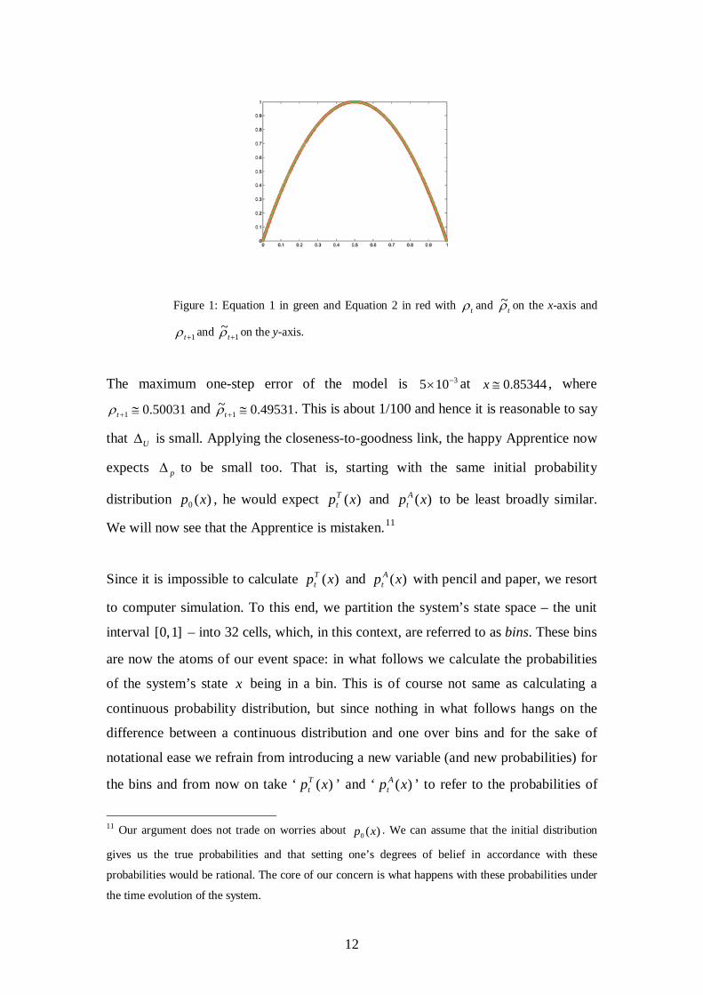
Figure 1 shows both TU and AU for 1.0=ε , making it obvious how small the

difference between the two is.

12

Figure 1: Equation 1 in green and Equation 2 in red with tρ and tρ~ on the x-axis and

1+tρ and 1~

+tρ on the y-axis.

The maximum one-step error of the model is 3105 −× at 85344.0≅x , where

50031.01 ≅+tρ and 0.49531~1 ≅+tρ . This is about 1/100 and hence it is reasonable to say

that U∆ is small. Applying the closeness-to-goodness link, the happy Apprentice now

expects p∆ to be small too. That is, starting with the same initial probability

distribution )(0 xp , he would expect )(xpTt and )(xp A

t to be least broadly similar.

We will now see that the Apprentice is mistaken.11

Since it is impossible to calculate )(xpTt and )(xp A

t with pencil and paper, we resort

to computer simulation. To this end, we partition the system’s state space – the unit

interval ]1,0[ – into 32 cells, which, in this context, are referred to as bins. These bins

are now the atoms of our event space: in what follows we calculate the probabilities

of the system’s state x being in a bin. This is of course not same as calculating a

continuous probability distribution, but since nothing in what follows hangs on the

difference between a continuous distribution and one over bins and for the sake of

notational ease we refrain from introducing a new variable (and new probabilities) for

the bins and from now on take ‘ )(xpTt ’ and ‘ )(xp A

t ’ to refer to the probabilities of

11 Our argument does not trade on worries about )(0 xp . We can assume that the initial distribution

gives us the true probabilities and that setting one’s degrees of belief in accordance with these

probabilities would be rational. The core of our concern is what happens with these probabilities under

the time evolution of the system.

13

bins. Similarly, a computer cannot handle analytical functions (or real numbers) and

so we represent )(0 xp by an ensemble of points. Specifically, we consider an

ensemble of 1024 initial conditions. We first draw a random initial condition

(according the invariant measure of the logistic map). By assumption this is the true

initial condition of the system at 0=t ; it is indicated designated by the cross in

Figure 2a. We then draw 1023 points randomly around the true initial condition

according to a Gaussian distribution. These 1024 points form our distribution, which

is shown in Figure 2a. Dividing the numbers on the y-axis by 1024 yields an estimate

of the probability for the system’s state to be in a particular bin.

We now evolve all these points forward both under the dynamics of the system and of

the model. Figures 2b-2d show how many points there are in each bin after two, four

and eight weeks respectively. Again, dividing these numbers by 1024 gives )(xpTt

and )(xp At at 2=t , 4=t and 8=t .

(a) (b)

(c) (d)

Figure 2: The evolution of the initial probability distribution under the Apprentice’s

approximate dynamics (green) and the Demon’s true dynamics (red). The crosses mark

the true initial condition and their time evolutions.

14

While the two distributions overlap relatively well after two and four weeks, they are

almost completely disjoint after two months. Hence, these calculations show the

failure of the closeness-to-goodness link because we have case where the smallness of

U∆ does not imply p∆ is small too for all t ; in fact for 8=t p∆ is as large as can be

because there is no overlap at all between the two distributions.12

This shows that even if a non-linear model is extremely close to the true dynamics

(remember that the maximal one step-error is 3105 −× !), then predictions, probabilistic

and deterministic alike, can break down. Hence, simply moving an initial distribution

forward in time under the dynamics of a good model need not yield decision-relevant

outcomes.

One could object that the presentation of our case is biased in various ways. The first

alleged bias is the use of an eight week forecast: had we used two or four week

forecasts instead, the apprentice’s endeavours would have been successful. While this

may be true in our specific example, in real modelling scenarios we cannot compare

model outputs with the true occurrences and affirm that we are fine at 4=t . In fact, if

we were able to calculate the evolution of the probabilities under the true dynamics

we would not use a model in the first place! Outside the thought experiment, the only

thing we have is the model, which we know to be imperfect in various ways. Our tail

shows that model-probabilities and probabilities in the world can come unstuck

dramatically, and as long as we have no means of telling when this happens, we’d

better be on guard.

Another alleged bias is the choice of the particular initial distribution shown in Figure

2a. This distribution, so the argument goes, is cleverly chosen to drive our point home

but most other distributions would not be misleading in such a way. Our results, so

the argument continues, only shows that unexpected results can occur every now and

then, but that is not enough for a wholesale rejection of the closeness-to-goodness

link.

12 We are operating with an intuitive notion of difference here; below we make this notion precise in

terms of relative entropy.

15

There is of course no denying that the above calculations rely on a particular initial

distribution, but that realisation does not rehabilitate the closeness-to-goodness link.

We repeated the same calculations with 2048 different initial distributions (chosen

randomly according to the invariant measure of the logistic map), and so we obtain

2048 pairs of )(xpTt and )(xp A

t for 2=t , 4=t and 8=t . So far we operated with an

intuitive notion of overlap of two distributions. But in order to analyse the 2048 pairs

of distributions we need a formal measure of the overlap of two distributions. We

choose the so-called relative entropy, which is defined as:

dxpppppS T

t

AtA

tTt

At ∫

=

1

0

log:)|( ,

where ln is the natural logarithm (i.e. the logarithm to the base e).13 The integral of

course becomes a sum over the bins of the partition. The relative entropy provides a

measure for the overlap of two distributions. If the distributions overlap perfectly,

then Tt

At pp = and the entropy is zero; the more different the distributions, the higher

the value of )|( Tt

At ppS . Figure 3 shows a histogram of the relative entropy of our

2048 distributions.

Figure 3 – Histogram of the relative entropy of 2048 pairs of

distributions at 8=t .

13 For a discussion of relative entropy and information theory see (Curd and Thomas 1991).

16

The histogram shows that the Apprentice’s probabilities are in line with the Demon’s

only in about a quarter of the cases. Almost half of the pairs of distributions have

relative entropy 7 or more. The two distributions shown in Figure 2d have a relative

entropy of 8.23.14 So our histogram shows that at 8=t almost half of all distribution

pairs are as disconnected as the ones on Figure 2d, and hence are seriously

misleading.

Observing how probabilities come unstuck and calling distributions ‘off track’ and

‘seriously misleading’ has intuitive force, but what exactly is the real damage? To

answer this question we observe the Apprentice’s next endeavour. Still not convinced

by the Demon’s arguments he opens the Pond Casino. The Pond Casino functions like

a normal casino in that it offers bets at certain odds on certain events. Let A be an

event that can obtain in whatever game is played in the casino. The odds )(Ao the

casino offers on A is the ratio of payout to stake. If, for instance, the casino offers

2)( =Ao (‘two for one’), this means that a punter who bets £1 on A gets £2 back

when A obtains. Within the context of standard probability theory odds are usually

taken to be the reciprocals of probabilities: )(/1)( ApAo = . When flipping a coin, for

instance, the probability for heads is 0.5, and if you bet £1 on heads and win, you get

£2 back.15 The Apprentice follows this convention when converting the probabilities

of his model into odds. However, we emphasise that it is by no means necessary, or

even advantageous, to construe the relation between probabilities and odds in this way

and we will discuss alternatives in Section 7.

14 In our calculations the lowest probability we assign to a bin is 1/(1024*32) when there is no

ensemble member in the bin. If the true probability for that bin is 1, then the entropy would be 10.4.

Hence 10.4 is the maximum value of the entropy.

15 We use so-called odds-for throughout this paper. They give the ratio of total payout to stake. Odds-to

give the ration of net gain to stake (net gain is the payout minus the stake paid for the bet). Odds-for

and odds-to are interdefinable: if the odds-for for an event are ba / , then the odds-to are bba /)( − .

Since in this case odds-for are equal to )(/1 Ap , the odds-to are )(/)(1 ApAp− which is equal to

)(/)( ApAp ¬ , where A¬ is ‘not A ’.

17

The Apprentice’s casino is different from a normal casino in that the events on which

punters can place bets are not outcomes of the spinning of a roulette wheel or any

other traditional gambling device but future values of tρ . The Apprentice takes the

above division of the unit interval into 32 bins and takes these as the basic events

(corresponding to the slots on the roulette wheel in a ‘normal’ casino). He then offers

odds on these events based on )(xp At

More specifically, playing a ‘round’ in the Pond Casino at time t amounts to placing

a bet at t on bin iB , where the outcome is whether the system is in iB at 4+t (that

is, a round is played with a four-step forecasts). So if you bet, say, on 31B at 3=t the

you win if 7=tρ is in 31B . The odds offered by the casino on this event are determined

by a four-step forecast using )(xp At . By contrast, the even that obtains at 7=t is

determined according to the true distribution )(xpTt because what happens in the

pond is of course not influenced by the Apprentice’s predictions.

Now a group of nine punters enters the casino. Each has £1000 and they adopt a

simple strategy. In every round, the first punter bets 10% of his wealth of on events

with probability in the interval ]1,5.0( . We call this strategy fractional betting (with

10/1=f ) for the probability interval ]1,5.0( .16 The second punter does the same

with events with probability in ]5.0,25.0( , the third with event with probability in the

interval ]25.0,125.0( , and so on with ]125.0,16/1( , ]16/1,32/1( , ]32/1,64/1( ,

]64/1,128/1( , ]128/1,256/1( , ]256/1,0[ . The minimum bet the casino accepts is £1;

so if a punter’s wealth falls below £1 he is effectively broke and can’t play any more.

We now use the same initial distribution as above (shown in Figure 2). The Pond

Casino offers odds on the events based on the Apprentice’s calculations; i.e. based on

)(xp At . The outcomes of bets are of course determined by the true dynamics; i.e.

)(xpTt . We now generate a string of outcomes based on )(xpT

t and trace the punters’

16 The argument does not depend on fractional betting, which we chose for its simplicity. Our

conclusions are robust in that they hold for other betting strategies (Smith et al. 2012).

18

wealth, which as a function of the number of rounds played. The result of this

exercise is seen in Figure 4.

Figure 4 – Wealth of punters as a function of the number of rounds played.

We see that the punters have the time of their lives. Three of them make huge gains

pretty soon, and further four follow suit a bit later. After 2500 rounds, seven out of

nine punters have increased their wealth at least ten-fold, while only two of them have

gone bust. So the punters take a huge amount of money off the casino!

One could now try to mitigate the suggestive force of this course of events by

pointing out that it may well be an incident of bad luck for the casino: we generated a

string of events by random draws according to )(xpTt , but this allows for the unlikely

events to happen and so the casino lost all that money is in fact due to a low

probability event happening.

To counter this objection we consider the same 2048 randomly chosen initial

probability distributions as above. For each of these we let the game take place as

before. If the above was a rare special event, then one would expect to see different

results in the other 2047 runs. Since producing another 2048 plots like the one seen in

Figure 4 would be rather cumbersome and since our focus is on the long term fate of

the casino, we assume that casino starts with a capital of £1,000,000 and now

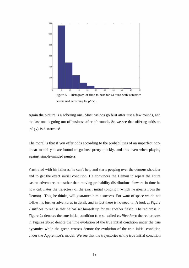
calculate the time-to-bust. Figure 5 shows how the casinos are doing.

19

Figure 5 – Histogram of time-to-bust for 64 runs with outcomes

determined according to )(xpTt .

Again the picture is a sobering one. Most casinos go bust after just a few rounds, and

the last one is going out of business after 40 rounds. So we see that offering odds on

)(xp At is disastrous!

The moral is that if you offer odds according to the probabilities of an imperfect non-

linear model you are bound to go bust pretty quickly, and this even when playing

against simple-minded punters.

Frustrated with his failures, he can’t help and starts peeping over the demons shoulder

and to get the exact initial condition. He convinces the Demon to repeat the entire

casino adventure, but rather than moving probability distributions forward in time he

now calculates the trajectory of the exact initial condition (which he gleans from the

Demon). This, he thinks, will guarantee him a success. For want of space we do not

follow his further adventures in detail, and in fact there is no need to. A look at Figure

2 suffices to realise that he has set himself up for yet another fiasco. The red cross in

Figure 2a denotes the true initial condition (the so-called verification); the red crosses

in Figures 2b-2c denote the time evolution of the true initial condition under the true

dynamics while the green crosses denote the evolution of the true initial condition

under the Apprentice’s model. We see that the trajectories of the true initial condition

20

under the two dynamical laws is vastly different, and any prediction generated with

the model is, once again, seriously misleading.

So making forecasts with exact initial conditions rather than probability distributions

does not convert failure into success. The lesson to be learned is that nothing short of

the Demon’s capabilities will deliver what we are after: reliable forecasts.

4. From Example to Proof

An obvious line of criticism would be to argue that the problems described in the last

section are specific to the logistic map and do not generalise to other systems, and in

particular don’t generalise to interesting cases like climate models. We are, so the

argument goes, guilty of overselling our case when making claims about all non-

linear models on the basis of the most specific of cases, and a more tempered attitude

to wards inductive generalisation would urge caution. Unfortunately the above

problems cannot be dismissed so easily. In fact there is a general mathematical

argument for the conclusion that the above phenomena occur in all structurally

imperfect non-linear models.17

Let us return to the scenario of Section 2 and consider the true Ttφ and the

Apprentices idealised Atφ , and, as before, we assume that A

tφ is idealised and

simplified and hence not identical with Ttφ . Also in keeping with the above set-up, let

us assume that there is finite observational resolution: we cannot observe the precise

initial condition but only assert that the system’s initial condition is somewhere in an

interval )(xI around the condition x which is the outcome of our measurement.18

States in )(xI cannot be distinguished by measurement in that that we cannot observe

17 What follows is a simplified version of the argument in (Judd and Smith 2004). See also (Smith

2002). Furthermore, in what follows we only consider parts of the state space that the systems actually

visit. 18 This is the most simple type of observational noise, arguments below generalise to more complex

forms of observational noise.

21

whether the system is in y or z for any )(, xIzy ∈ . We call such states non-

distinct.19

Now consider )(xIy∈ , xy ≠ at a given time, say 0t ; that is, x and y are non-

distinct at 0t . We can now ask the question whether x and y remain non-distinct in

the future if x evolves under the dynamics of the target system and y under the

dynamics of the model. Let us denote the set of states that are thus non-distinct by

)(xI∞ . More formally: )(xIy ∞∈ iff )(xTtφ and )(yA

tφ are non-distinct for all 0≥t .

Judd and Smith (2004) prove a theorem making a very general statement about

pseudo-orbits of imperfect systems. The theorem itself need not occupy us here. What

matters to us is that it implies what we call Proposition 1 (ibid., 231):

Proposition 1: For a chaotic model with structural model error the following

holds true: if there exists a non-empty )(xI∞ , then Ttφ and A

tφ are identical.

This is logically equivalent to the statement that if Ttφ and A

tφ are not identical then

there is no non-trivial )(xI∞ . If the model is not perfect there is no non-trivial set of

indistinguishable states. In other words: if the model is structurally imperfect, then ‘no

state of the model has a trajectory consistent with observations of the system’ (ibid.

228): the states in )(xI become distinguishable as time evolves.

In physical situations as the ones considered in Sections 2 and 3, the probability

distribution expresses the uncertainty about the system’s initial condition. The

conditions we are uncertain about are the ones we cannot distinguish by a

measurement. So if we determine that, for all practical purposes the initial condition is

x , we put a probability distribution over )(xI . The distribution in Figure 2a, for

instance, is a distribution over the indistinguishable states of the position

measurement. In keeping with the notation of Section 2, let us call this distribution

)(0 xp ; )(xpTt and )(xp A

t are then defined as before. The above theorem then has the

19 We use ‘non-distinct’ to avoid confusion because ‘indistinguishable’ is used in a technical – and

different – sense in (Judd and Smith 2004).

22

consequence that the relative entropy of the two distributions increases,20 and they

may even come unstuck in the way seen in Figure 2.

The theorem holds true under very general assumptions. In particular it holds for

Hamiltonian as well as for dissipative chaotic systems; and it holds true both for

discrete time evolutions of the kind discussed here and for continuous flows. This

drives the point home that the effects and problems described in Section 3 are not

specific to the logistic map and indeed occur in a vast class of systems.

5. Imperfect Models in Action

As we have briefly indicated above, the qualification that one must know the true

dynamics to make useful forecasts is more than academic hair-splitting. The scenario

we have discussed is a close cousin of many real-world research projects. In most

scientific scenarios the truth is beyond our reach and we have to rest content with an

approximation – it is a well-rehearsed truism that all models are wrong. Real scientists

are therefore often in the position of the freshman apprentice in that they produce

predictions with a less than perfect model. Some of these predictions are then used to

assess the risk of future outcomes, for instance when setting insurance policies or

assessing policy option. So insurers and policy makers are often like the owner of the

pond casino: they have to set premiums or make policies on the basis of imperfect

model outcomes. Of course scientists and insurers know that their models aren’t

perfect, but they nevertheless make predictions and set premiums using these models.

The tacit assumption behind this practice may be the closeness-to-goodness link: they

believe that if the model is close enough to the target system (which the models are

assumed to be), then its predictions are good enough inform the setting of insurance

premiums and policy making.

20 This is a direct consequence of the definition of the time-evolution of a distribution which we

mentioned above: )()]([:)( 00 iitt zpxpxp Σ==φ

23

Examples can be drawn from domains as different as load forecasting in power

systems (Fan and Hyndman 2012), inventory demand management (Snyder, Ord, and

Beaumonta 2012) and weather forecasting (Hagedorn and Smith 2009).

In these cases, and no doubt many others, probability distributions are moved forward

in time in the manner described above and hence there are serious worries about

whether these model outputs can be used as decision relevant probabilities. However,

the case we would like to highlight especially is climate change. For one, predicting

the world’s future climate is a modelling exercise par excellence. This case

particularly interesting also because unlike daily forecasting activities where one can

experience the success or failure of a forecasting system day after day, there is little,

arguably no, relevant out-of-sample verification for future climate change predictions.

For another, climate change is one of the important challenges of our time and so it is

important that forecasts on which many wide-ranging policy decisions are based be

reliable.

There is now a widespread consensus that the earth’s climate is warming up and that

human activities, in particular the burning of fossil fuels, are the main cause (Oreskes

2007; Dessler and Parson 2011, Ch. 3). But knowing that on the whole (or on

average) the climate is getting warmer is of limited use if we aim to design effective

adaptation strategies.21 The impact of climate change on humans (as well as other

organisms) occurs at a local scale, and so ideally we would like to know what changes

we have to expect in our immediate environment. For instance, how does the

precipitation change in London by the end of this century? The answer to questions of

this kind have significant implications, for instance, for the planning of water

reservoirs, agriculture and flood defences, and so having a reliable answer would

greatly aid policy makers (Smith and Stern 2011).

21 It may well be enough for mitigation: knowing that it happens is enough for not wanting to go there.

However, it is now widely acknowledged that the question we are facing can no longer be described as

an either-or question with mitigation and adaptation as alternatives. Since we are already in the midst

of climate change, some level of adaptation is unavoidable even if we still ought to aim at mitigating

against worse things happening.

24

A recent government-funded research project called United Kingdom Climate

Projections (UKCP) aims to answer exactly such questions by making high resolution

forecasts of the climate out to 2100. UKCP predicts, for instance, that there is a 0.5

probability for a 20-30% reduction in precipitation in London in 2080.22 How are

such predictions generated and how trustworthy are they?

This is the point at which high resolution general circulation models enter the scene.23

In the case of climate models X consists of relevant weather variables (such as air

temperature, precipitation, …), and tφ tell us how they change over time. When

described at that level of abstraction, one could be left under the impression that

climate models are rather simple things. It is important to counter this impression

before it gains traction. A full specification of the system’s state space would involve

giving the air temperature, precipitation, etc at every point on the surface of the earth!

It is not only a practical impossibility to obtain these data; it is also an impossibility to

store and process them with digital technology. So we discretise the state space,

meaning that we put a grid with a finite number of cells on X and represent the state of

an entire cell by one set of values for the relevant variables. The grid size is the length

of the sides of the cells. Typically the grid size used in a climate model is well over

100km. Covering the world with such a grid still leaves us an enormous amount of

data! Yet it is important to emphasise that the volume of numbers notwithstanding,

this is a rather coarse description. For instance, the weather in the entire city of

London is now represented by one set of numbers (one number for temperature, one

for precipitation, etc.).

The dynamics of the model raises further issues. The sheer scale and complexity of

the task makes it unavoidable that models are imperfect. In order to specify tφ we

have to make a number of strongly idealising assumptions: we distort important

aspects of the topography of the surface of the earth as the resolution of these models

does not allow for realistic mountain ranges like the Andes, does not resolve the

22 See http://www.ukcip.org.uk/wordpress/wp-content/UKCP09/Summ_Pmean_med_2080s.png;

retrieved on 12 October 2011. 23 For a general introduction to climate modelling see (McGuffie and Henderson-Sellers 2005); a

discussion of UKCP in particular can be found in (Frigg, Smith, and Stainforth 2012).

25

southern half of the state of Florida, many islands simply don’t exist, including small

volcanic islands chains easily visible in satellite photographs due to their interaction

with clouds, and of course clouds fields themselves are not modelled realistically.

Based on these idealising assumptions we can use basic physics (essentially fluid

dynamics and thermodynamics) to formulate the equations of motion for the

simplified earth’s climate system. These equations are non-linear and we cannot solve

them analytically. For this reason we resort to the most powerful computers available

to compute solutions. The result of these computer simulations is tφ .

It is practically impossible to specify the exact state of the earth-system at some time

0t because there is no measurement device that provides exactly true values and so

every measurement result comes with a certain margin of error.24 Climate models are

then used to turn these probabilities into predictions for the future. These models (e.g.

HadCM3) are de facto non-linear. So we are in the position that we have to use an

imperfect dynamical law to move current uncertainties forward in time, and for this

reason all the above worries arise. UKCP probabilities are formed in a more

complicated manner than by simply applying the Default Position; they are calculated

by combining outputs from multiple (imperfect) models using Bayesian methods.25

However, it is unclear why combining the outputs of several structurally imperfect

models in a complicated manner should make the problems we describe go away. In

the very least the burden of proof in this matter lies with those who wish to maintain

that this is the case. So there is a serious question whether these model outputs can be

trusted. When calculating, say, monthly precipitation in the 2080s based on climate

models we may well not fare better with our planning of flood provision and water

systems than the freshman apprentice with his casino!

24 Some would go even further and say that there is no exact initial condition because there is no such

thing as the true wind speed in a model grid point corresponding to central London! Whatever number

we settle on is an average of some kind or other; all we can truthfully say is something like ‘the wind

speed at a particular random location within that grid cell is likely to lie within a certain range’. For

what follows nothing depends on the issues of whether imprecise initial conditions are the result of

practical or in-principal limitations. 25 http://ukclimateprojections.defra.gov.uk/23239 and http://ukclimateprojections.defra.gov.uk/23210.

26

6. Attempts at Exorcism

The main consequence of the above argument is that there are serious questions

concerning a widely used modelling methodology. The first reaction of those trying to

help policy makers is therefore to question the soundness of our argument. In this

section we discuss several attempts to do so. We deal with them in ascending order of

severity and conclude that they prove unsuccessful. We concentrate on the climate

case; similar arguments can be made for other modelling context and the replies

remain the same mutatis mutandis.

6.1 Get Rid of Non-Linearity

A quick and simple reply is to say that if non-linearity causes so many difficulties,

then should just get rid of it and construct a linear model instead. This reply is

confused. We don’t construct non-linear models because we for some reason like

them – the choice between linear and non-linear models is not like the one between

strawberry and vanilla ice cream. Non-linearity is forced upon us by nature because

many processes in nature are non-linear (phase transitions of water are but one

example), or at any rate are better modelled by nonlinear mathematical equations than

linear ones So one can’t simply choose to have a linear rather than a non-linear model.

A more nuanced version of this objection would be that climate is not linear tout

court, but the non-linearities in climate systems are small and to make predictions on

the time scale of interest (50-100 years), the system can treated as linear (i.e. it can be

linearised) without loss. This does not seem to be plausible either. To begin with, it

would be incomprehensible why scientists put immense resources (in terms of

finances and research time) towards programming and running super computers to

numerically integrate nonlinear equations if these equations could effectively be

linearised and hence dealt with much more easily. A look at actual examples soon

reveals that there is nothing irrational about scientists use of resources. Essential

variables of climate models are strongly non-linear and we cannot simply linearise a

nonlinear model (the change in albedo due to the transition from snow to water as

tenmperature passes through zero degrees Celsius is a case in point).

27

6.2 Climate is About Averages

The next line of defence to fall is that while it is true that weather models are non-

linear (and hence suffer from the problems we describe, climate science is about

averages and averages obey linear laws.

This objection is mistaken twice over. First, climate is not about averages. How

exactly to define climate is an interesting question, but it has been pointed out

variously that it ought not be equated with averages. As early as 1938, Kendrew

insisted that there was more to climate than ‘mean conditions’; in 1959 the first

edition of the Glossary of the American Meteorological Society defined the climate as

‘the long term manifestations of weather, however they may be expressed’; and in

1982 Lamb bemoaned that climate was ‘wrongly defined in the past as just “average

weather”.26

Second, even if climate science dealt with averages, there would be no guarantee that

averages are governed by linear equations. There is nothing in the notion of an

average that makes it subject to linear laws. Indeed, there is no guarantee that

averages are governed by any law at all! Usually many states of a system are

compatible with a certain average and so there is need not be a dynamical law that

governs averages as such.

There is, however, a more sophisticated argument along the same lines. The challenge

now is that we are playing fast and loose with the notion of prediction. While the

freshman apprentice wants to predict what happens exactly two months from now, the

above-mentioned climate prediction is for the 2080s, an entire 10 year period. So we

seem to be comparing apples and oranges because in the climate case we are

interested in a decadal average and not a prediction for a specific instant of time as in

the fish case. Once this is realised, so the objection concludes, our argument loses its

bite.

26 For references an a further discussion of the relation between weather and climate see (Smith and

Stainforth 2012)

28

Implicit in this rejoinder is the assumption that averaging over a period makes the

above problems go away. This need not be so. In a simple system like the logistic map

is may well be the case that over a sufficiently long period the initial distribution

traces the entire state space in a way that makes averages insensitive towards the

actual trajectory taken (for instance, it would not matter whether the distribution

peaks in ]5.0,0[ at 4=t and in ]1,5.0( at 8=t or vice versa). In models with literally

tens of thousands of dimensions (such as climate models), however, the distribution

need not trace out the entire state space during the relevant time period, and so model

averages may well differ from their real world counterparts.

Furthermore, the situation in UKCP predictions is not as good as the critic assumes.

What looks like a decadal average is in fact an annual distribution. This is not so

different from weekly predictions in the fish model. Other predictions made by UKCP

are even more precise, e.g. the forecasts for the hottest day in August of a particular

year. So what UKCP provides are not long term averages and hence an appeal to

averages does not help circumventing the difficulties we describe.

6.3 Quibbles about time scales

We argue that structural model error leads to getting the distribution wrong, and that

once this has occurred one will have averages and extremes wrong. This argument is

as unassailable as it is simple. The only way out is to respond that the time scale for

this to occur is much larger than the time scale of interest.

In some cases this seems to be the right response. In weather forecasting, for instance,

we are mainly interested in predicting the immediate future and hence limiting model

runs to the short term is the right thing to do. But this response does not seem to work

in all cases. In both weather and climate modelling, for instance, we are also

interested in the medium or long term behaviour and so we cannot limit predictions to

short lead times. Of course what counts as short-term or long-term is relative to the

29

model and it could be the case that by standards of the relevant climate models a

prediction for 2080 is still a short term prediction.

We are doubtful that this is the case. Indeed, it would be surprising if predictions for

2080 would turn out to be short term even by the lights of a model used to make that

prediction. Our scepticism is rooted in the fact that state of the art climate models

differ in terms of their performance over the past century. The (empirically measured)

change in global mean temperature over the last century was approximately 0.5

centigrade, but the systematic error in model simulations is around 3 centigrade

(Smith 2012). Furthermore, currently available models differ significantly in their

medium and long term predictions. Comparing predictions for the relative changes in

precipitation for the period 2090–2099 (relative to 1980–1999) of different models

shows that for several parts of the world – Spain, the southern part of the United

States and substantial portions of Latin America and Africa – less than 66% of the

models considered agree even on the sign of the change! Some models say it will rain

more and some say it will rain less (IPCC2007 Figure SPM.7). So we know that the

details of the models have a significant impact on expected results and hence there is

no reason to assume that projections of 60 to 80 years are of a kind that is

unproblematic.27

Another challenge along the same lines argues for the opposite conclusion: what we

are interested in is long term behaviour and so we do not need detailed predictions at

all and can just study the invariant measure of the dynamics (in this context often

referred to as the climatology). The invariant measure reflects a system’s long term

behaviour because the initial distribution “washes out”, and hence it is immaterial

where we started. It then doesn’t matter that for medium times the distributions look

different because we are simply not interested in them. This view gains support from

the fact that we seem to have revealed only half of the truth in Section 3. If we

continue evolving the distribution forward to higher lead times rather than stopping at

8=t we find that the two distributions start looking similar again and, moreover, that

they start looking very much like the invariant measure of the dynamics (Lichtenberg

and Liebermann 1992, 501). This is shown in Figure 6 below. Hence, it seems that in

27 See (Smith 2002).

30

the long run all we need to make reliable predictions is the invariant measure and we

can forget about the ‘medium term aberrations’ seen in Figure 2.

Figure 6 – The same scenario as the one seen in Figure 2 but for lead times 16=t and 32=t .

Implicit in this proposal is the assumption that the invariant measures of similar

dynamical laws are similar, because unless Equations 1 and 2 have similar invariant

measures there is no reason to assume that adjusting beliefs according to the invariant

measure is less misleading than adjusting them according to )(xpmt . However, it is at

best unclear whether this is so. Even though Figure 6 suggests that this is so in the

case of the logistic and the quartic map, there is no reason to assume (let alone a

proof) that in general invariant measures have this property. Nonlinear systems are

not expected to be structurally stable in general, and invariant measures of nearby

systems are not expected to be similar.

Furthermore, unlike our pond, the world’s climate system is not a stationary system.

But transient systems do not have invariant measures, which forecloses a response

along the above lines. A response to this is that we are overstating the transient

character of the climate because, one of the most prominent models of the worlds

climate, namely HadCM3, in fact has an attractor. There is an invariant measure on

the attractor and so we can do exactly what was suggested above just with the

qualification that we study the invariant measure on the attractor.

HadCM3’s attractor is a red herring for several reasons. First, there is no proof that

such an attractor exists. If we focus on the model as implemented on a digital

computer we are bound to find recurring phenomena, but these need not be indicative

31

of an attractor. A digital computer is finite machine with a finite number of states and

hence sooner or later the same states are revisited – so what we find are periodic

orbits of the machine. If we look at the full equations of the model, then we simply

don’t know whether there is an attractor. Second, even if there is an attractor, this is

so only for fixed carbon dioxide levels. However, a core issue in any discussion of

climate change is that carbon dioxide levels increase and hence whether there is an

attractor for fixed levels is a somewhat moot point. Third, even if we focus on the

scenario with fixed carbon dioxide levels, it will take the system thousands of years to

reach the attractor (Smith 1987), which is too long to be of interest to humans. Lastly,

HadCM3 is only one model in a class of climate models, and different models will

have different attractors (if they have attractors at all), and predictions generated from

studying these attractors need not coincide (recall the above point about model

discrepancies for relative changes in precipitation).

6.4 Probabilism Reloaded

So far we have shown that making probabilistic forecasts with structurally imperfect

models can be seriously misleading. But have we not just used probabilities in a bad

way? An immediate response to the above problem would be to point out that by only

using one particular model to make generate predictions we have implicitly assigned

probability one to that model. Given that we have no reason to assume that this model

is true – indeed, there are good reasons to assume that it’s not! – this confidence is

misplaced and one really ought to take uncertainty about the model into account. This

can be done by using probabilities: put a probability measure on the space of all

models which expresses our uncertainty about the true model, generate predictions

with all those models, and take some kind of weighted aggregate of the result. This, so

the argument goes, would avoid the above problem which is rooted in completely

ignoring second order uncertainty about models.

Unfortunately this strategy does not work. Setting aside the fact that it is practically

infeasible to generate predictions with an entire class of models, there are theoretical

limitations that ground the project. The first problem is that it is not clear what the

relevant model class would be. This class would contain all possible models of a

32

target system (such at the earth’s atmosphere). The nice phrase ‘all models’ masks the

fact that mathematically this class is not defined, and indeed it’s not clear whether it is

definable at all. The second problem is that even if one could construct such a class in

one way or another, there are both technical and conceptual problems with putting an

uncertainty measure on this class. The technical problem is that the relevant class of

models would be a class of functions and function spaces do not come equipped with

measures. In fact, it is not clear how to put a measure on function spaces.28 The

conceptual issue is that even if the technical problem could be circumvented

somehow, what measure would we chose? The model class will contain an infinity of

models and it is at best unclear whether there is a non-arbitrary measure on such a set

that reflects our uncertainty about model choice. For these reasons this response does

not seem to be workable.29

7. Sustainable Odds

So far we have discussed problems with imperfect models and pointed out that there

is no easy fix. One natural reaction would be to throw in the towel and conclude that

the best would be not to use such models at all. This would be throwing out the baby

with the bathwater. As we have seen above, in some cases at least the model provides

insight (for instance for 2=t and 4=t in Figure 3). So the question is: how can we

use the information in the model without being too dramatically misled in the cases in

which the model goes wrong. This question has no easy answer because unlike in our

thought experiment, in which we have access to the true dynamics, in every day

science we don’t know what the truth is and so we cannot simply compare our models

with the true dynamics (indeed, if had access to the truth the model would be

superfluous!). So in everyday science we are like the freshman apprentice without the

Demon. So what should the apprentice do to improve his casino? In this section we

propose the use of non-probability odds as one way around the problem. We introduce

28 This is a well-known problem in the foundation of statistical mechanics; see (Frigg and Werndl). 29 A suggestion somehow along the lines of the above is (Murphy et al. 2007); however, they conclude

that all one can derive is a lower bound and not full probabilities (ibid., 2011).

33

these in Section 7.1. In Section 7.2 we show that they indeed solve the above

problem, and we end with a few cautionary remarks about decision theory (Section

7.3).

7.1 Non-Probability Odds

As we have seen above, the odds )(Eo the casino offers on an event E is the ratio of

total payout to stake (where ‘total’ indicated that the payout includes the initial stake).

If there is a probability )(Ep for E , then the odds on E are the reciprocals of the

probabilities: )(/1)( EpEo = . From this it follows, trivially, that the inverse of a

complete set of odds adds up to one. In more detail, let }...,,{: 1 nEE=α be complete

set of events (in the sense that any event that can possibly occur is in α ),30 and let

)( iEo , ni ...,,1= , be the odds on all the events in α . Then we have

1)(

11

=∑=

n

i iEo. (3)

So far we have taken probabilities as the starting point and talked about odds as if

they were the derivative quantities. This need not be so: we can just as well take odds

as out starting point, and say that the longer the odds for an event iA , the more

surprising it is if the event occurs. Odds thus understood do not necessarily have any

connection to probabilities. Considering again the complete event set of events α ,

and let )}(...,),({: 1 nEoEo=ω be the complete set of odds for α . The )( iEo simply

reflect how surprising or unsurprising we consider certain events to be. We then say

that the odds ω are probability-odds if, and only if, ω satisfies Equation 3; they are

non-probability odds otherwise.31

Let us then call )(/1:)( ii EoE =π the betting quotients on iE . The π are “probability-

like” in that they are numbers between zero and one, with one indicating that the 30 We only consider discrete and countable event spaces. 31 Non-probability odds have been introduced in (Judd 2007) and (Smith 2007).

34

obtaining of an event is no surprise at all and zero representing complete surprise. If

odds are probability-odds, then )()( ii EpE =π .32

Non probabilistic odds are interesting. On the one hand they immediately induce cold

sweat in everybody interested in rational decision because there are formal results for

the conclusion that one is irrational (one faces guaranteed loss) if one accepts bets that

do not respect probability calculus - we briefly come back to these results below in

Section 7.3. On the other hand they are ubiquitous in every day situations. Real

casinos, for instance, do not offer probability-odds. Assuming that they have true

probabilities for simple gambling devices like dice and roulette wheels, offering

probability-odds would result in them breaking even in the long run, but to run the

casino sustainably also in the short and medium term, they shorten the odds. The

American roulette wheel has 36 numbers plus 0 and 00. Let us assume that the wheel

is perfect (and is spun so that no one can calculate outcomes by taking the initial

condition and the speed into account). Then the probability for certain slot, say #23, is

38/1 and hence 38)]23#(/1[)23#( == po . However, all bets are paid at odds 36 , i.e.

odds that would be true fair the wheel only had 36 numbers. So we have

)#23()#23( π<p , and hence 1)(/11

>∑=

n

iiEo for the odds offered by the casino.

For a commercial casino shortening odds is simply a business decision. The main

point of this section is the shortening odds can also be used as a tool to guard against

the unquantified risk catastrophic loss (of the kind we have seen in Section 3), and the

amount of shortening can be regarded as a measure for our uncertainty about the

model – i.e. the apprentice’s uncertainty about his model outputs.

7.2 Non-probability Odds in Action: Threshold and Damping

Let us continue our thought experiment. After the first casino fiasco the Apprentice

wants to try again, but this time without going bust. From his last experience he

32 Sometimes the π are called implied probabilities. This nomenclature is misleading because, as we

have just seen, not all π are propbabilities.

35

knows that using probabilistic odds set according to )(xp At is recipe for disaster. So

he decides to shorten his odds to guard against loss. Of course you can always guard

against loss by not paying out any net gain at all and merely returning the stake to

punters when they win (i.e. by setting all 1)( =iEo ). This, however, is not interesting

to punters and they would not play in his new casino. So he aims to offer a game that

is as attractive as possible by offering odds that are as long as possible, but only so

long that he does not unexpectedly go bust.

There are different ways of shortening odds. Perhaps the simplest way is to impose a

threshold τ on the )( it Eπ : )()( iAtit EpE =π if τ>)( i

At Ep and τπ =)( it E if

τ≤)( iAt Ep , where τ can be any real number so that 10 ≤≤τ . We call odds thus

calculated threshold-odds. For the limiting case of 0=τ the )( it Eπ become

probabilities and the respective odds probabilistic odds. It is important to emphasise

the threshold rule applies to all possible events and not only the atoms of the partition,

the idea being that one simply does not offer π ’s smaller than τ no matter what the

event under consideration is. In particular, the rule applies to events and their

negation. If, for instance, we set 2.0=τ and have 95.0)( =iAt Ep (and hence, by the

axioms of probability 05.0)( =¬ iAt Ep ), then 95.0)( =it Eπ and 2.0)( =¬ it Eπ , where

iE¬ is the negation of iE (i.e. the non-occurrence of iE ).

This move is motivated by the following observation. In Figure 2 we see that if the

two distributions we are offering, based on Atp very long odds on events that are in

reality (i.e. according to Ttp ) very likely to happen; that is, we wrongly regard likely

events as unlikely and therefore offer long odds on them. Putting a threshold on the

)( it Aπ amounts to limiting the length of odds and so one limits the amount one

amount one pays out for likely events that one wrongly regards as unlikely.

We now repeat the scenario of Figure 4 with one exception: the Freshman apprentice

now offers non-probability odds with a thresholds of 05.0=τ , 1.0=τ and 2.0=τ .

The result of these calculations is shown in Figure 7a, 7b and 7c respectively.

36

(a) (b) (c)

Figure 7 – Wealth of punters as a function of the number of rounds played with the casino

offering non threshold-odds with thresholds of 0.05, 0.1 and 0.2.

In Figure 7 we see that this strategy is a success. Already a very low threshold of

05.0=τ undercuts the success of five out of seven punters, and only two still manage

to take money off the casino. A slightly higher threshold of 1.0=τ brings the number

of successful punters down to one. For . So for 2.0=τ the Freshman apprentice

achieves his goal of running a sustainable casino.

The second way of shortening odds is damping. On this method the betting quotients

are given by )](1[1)( iAtit EpE −−= βπ , where the damping parameter β is a real

number 10 ≤≤ β . We see that for 1=β the tπ are probabilities. We call odds thus

calculated damping-odds. We now repeat the same calculations as above and the

results are very similar indeed. For 95.0=β only two punters succeed (indeed the

same two as above). With a slightly stronger damping of 9.0=β only one is still

winning (again the same as above), and for 8.0=β all punters are either losing or not

playing at all (because no bets in their range are on offer).

The moral of this last part of our tale of the Demon and his apprentice is that by

shortening odds either by introducing a threshold or by damping one can guard

against unexpected losses.

Furthermore we can regard the amount of deviation of the ‘shortening parameters’

from their ‘probability limits’ (i.e. the deviation of τ from zero and of β from one)

37

as a measure of how the model uncertainty: the further away the parameters are from

their probability limits the more uncertain we are about the model.

Before moving on we briefly want to continue the discussion in Section 4 and point

out that also this last part of our take is closer to reality than it seems. The sustainable

yet interesting casino is modelled on a cooperative insurance company. Rather than

playing for gain, the ‘bets’ placed are insurance policies they buy to compensate for

losses suffered should certain events happen. What makes our insurance a cooperative

insurance is its attempt to offer has high a payout as possible (to compensate its

clients as best as possible), but only to the point that it operates in a sustainable way

(an insurance company that goes bust unexpectedly is of little use). So our non-

probability odds casino has a close real-world cousin, and the morals drawn above are

relevant beyond the tale about Laplace’s Demon.

7.3 Epistemology, Not Decision Theory

So far we have seen that one is bound to lose money when betting on imperfect

model-probabilities. The conclusion of our argument might be seen as a decision

theoretic one: that is, that it is pragmatically advantageous to adopt non probabilistic

odds. This is not the interpretation we favour. We prefer to see it as an

epistemological argument, albeit one that involves talk of betting. We are not making

any decision theoretic assumptions in coming to our conclusions. Talk of casinos,

betting and going bust, helps putting an epistemic problem into focus – the main point

is that the pragmatic flaw (going bust) points to an epistemological flaw in the agent’s

representation of belief.

Needless to say, the use of non-probability odds raises a host of issues. How exactly

should non-probability odds inform decision making? Presented with non-probability

odds (or equivalently: betting quotients), what decision rules should we apply? These

important questions for decision theory and rational choice, but we cannot discuss

these here.

38

An attempt to dismiss these issues quickly might be to try to bring these issues back

into well charted territory by denying that non-probability odds are really sui generis

items. Regarding them as such, so the argument goes, is a red herring because even if

we have odds whose inverses don’t add up to one it is trivial to renormalise them and

we then retrieve the homely probabilities for which there are well worked out decision

theories. Renormalisation amounts to multiplying all odds with )(\1: ∑= iEoυ , or,

equivalently, all π with υ/1 .

Unfortunately things are not as simple as that because the π do not satisfy the axioms

of probability even if they add up to one. The problem is that non-probability-odds do

not respect the symmetry between betting for and betting against that is enshrined into

probabilities. For probabilities we have 1)()( =¬+ EpEp for any event E (where

E¬ is the non-obtaining of E ). Non-probability odds need not add up to one:

)()( EE ¬+ππ can take in principle take value 1≥x . This can be easily seen when

calculating non-probability odds as in the first of the above examples. Consider three

events with respective probabilities of 0.95, 0.01 and 0.04. It is easy to see that

35.1=υ . We represent the values (all rounded to two digits) of these probabilities as

well as the non-probability odds and the renormalized nonprobability-odds Rπ in the

following chart:

1E 2E 3E 1E¬ 2E¬ 3E¬

p 0.95 0.01 0.04 0.05 0.99 0.96

π 0.95 0.2 0.2 0.2 0.99 0.96

Rπ 0.7 0.15 0.15 0.15 0.73 0.71

We see that the Rπ for 1E , 2E , and 3E add up to unity as one would expect from

probabilities, and yet 1)()( ≠¬+ ii EpEp for all i . For this reason the Rπ are not

probabilities, and renormalising is not an easy route back into the territory of

probabilism.

We would not like to leave the issue without a brief remark about Dutch books. One

might worry that our freshman apprentice, with his non probabilistic odds, is subject

39

to a Dutch book. That is, one might worry that a smarter bettor might be able to

guarantee to make money out of the apprentice by buying a set of bets that guarantee

the bettor a sure gain, whatever happens. This is not the case. This is for the same

reason that casinos can’t be Dutch booked. That is, you cannot bet against an event

happening. Likewise, our apprentice is only offering bets on, not bets against events

(Bradley 2012). This is not the place to discuss this point further.

8. Conclusion

We have argued that the combination of non-linear dynamics and model imperfection

is a poison pill in that it shows that treating model outputs as probabilistic predictions

can be seriously misleading. At some level, probabilistic forecasts are therefore

unreliable and do not provide a good guide for action.

This raises two questions. The first concerns the premises of the argument. The model

being non-linear has been an essential ingredient of our story. While this assumption

is realistic in that many relevant models have this property, there is still a question

whether the effects we describe are limited to non-linear models. Arguably, if the

world was governed by linear equations, then imperfect linear models might perhaps

not suffer from the effects we discuss. One might like to avoid the assumption that the

world is governed by any equations, of course, but the relevant point here is the role

of model imperfections: a linear model will suffer from these effects if its

imperfections are were nonlinear. The model being linear does not remove the

difficulty we note. And of course, in practice the best models are often not linear, nor

are the relevant laws of physics.

The second question is what conclusion we are to draw from the insight into the

unreliability of models. An extreme reaction would be to simply get rid of them. But

this would often amount to throwing out the baby with the bathwater because, as we

have seen, in the short run model results are roughly correct, and even in the medium

term about one third of the cases the model indicates usefully. This raises several

questions. The first is: how long is long? As we have indicated in Section 6, there

probably will be no general answer, but there may be answers in particular cases. So

40

future research may want to pay more attention than it has done so far to the issues of

estimating the time span of reliable prediction. The second question is how we can

use the model when it provides insight while guarding against damage when it does

not. Finding a way of doing this is a challenge for future research. We have indicated

that one way possible route could be to use non-probability odds, but more needs to

be said about how these can be used to provide decision support, and there may be

altogether different ways of avoiding the difficulties we sketch.

Acknowledgments

We would like to thank Reason Machete, Gregor Betz, and Joel Katzav for helpful

discussion and/or comments on earlier drafts. We would like to thank audiences in

Athens, Bristol, Ghent, Nancy, London, Paris, and Toronto for valuable discussions.

This research was supported by the Centre for Climate Change Economics and Policy,

funded by the Economic and Social Research Council and Munich Re. Smith would

also like to acknowledge support from Pembroke College Oxford. Frigg would like to

acknowledge support from the Spanish Ministry of Science and Innovation through

the project FFI2008-01580.

Bibliography

Allen, M. R., and Leonard A. Smith (1996), "Monte Carlo SSA: Detecting irregular oscillations in the presence of coloured noise", Journal of Climate 9 (12):3373-3404.

Arnold, Vladimir I., and André Avez (1968), Ergodic Problems of Classical Mechanics. New York and Amsterdam: W. A. Benjamin.

Bradley, Seamus (2011), "Scientific Uncertainty: A User’s Guide", Grantham Institute on Climate Change Discussion Paper 56 (available at http://www2.lse.ac.uk/GranthamInstitute/publications/WorkingPapers/Abstracts/50-59/scientific-uncertainty-users-guide.aspx).

——— (2012), "Dutch Book Arguments and Imprecise Probabilities ", in Dennis Dieks, Wenceslao Gonzalez, Stephan Hartmann, Michael Stoeltzner and Marcel Weber (eds.), Probabilities Laws and Structures, Berlin Springer, 3-17.

Curd, Thomas M., and Joy A. Thomas (1991), Elements of Information Theory. New York: Wiley.

41

Dessler, Andrew, and Edward A. Parson (2011), The Science and Politics of Climate Change. 2nd ed. Cambridge: Cambridge University Press.

Fan, Shu , and Rob J. Hyndman (2012), "Short-Term Load Forecasting Based on a Semi-Parametric Additive Model", IEEE Transactions on Power Systems 27 (1):134-141.

Frigg, Roman (2010), "Fiction and Scientific Representation", in Roman Frigg and Matthew Hunter (eds.), Beyond Mimesis and Convention: Representation in Art and Science, Berlin and New York: Springer, 97-138.

Frigg, Roman, Leonard A. Smith, and Dave A. Stainforth (2012), "The Myopia of Imperfect Climate Models", forthcoming in Philosophy of Science.

Frigg, Roman, and Charlotte Werndl "Demystifying Typicality", Philosophy of Science forthcoming.

Hagedorn, R., and Leonard Smith (2009), "Communicating the Value of Probabilistic Forecasts with Weather Roulette", Meteorological Applications 16 (2):143-155.

Judd, Kevin (2007), "Nonprobabilistic Odds." Under Review. . Judd, Kevin, and Leonard A. Smith (2004), "Indistinguishable States II: The

Imperfect Model Scenario", Physica D 196:224-242. Laplace, Marquis de (1814), A Philosophical Essay on Probilities, Dover Edition

1995. New York: Dover. Lichtenberg, Allan J., and Michael A. Liebermann (1992), Regular and Chaotic

Dynamics. 2nd ed. Berlin and New York: Springer. McGuffie, Kendal, and Ann Henderson-Sellers (2005), A Climate Modelling Primer.

3rd ed. New Jersey Wiley. Murphy, J. M., B. B. B. Booth, M. Collins, G. R. Harris, D. M. H. Sexton, and M. J.

Webb (2007), "A Methodology for Probabilistic Predictions of Regional Climate Change for Perturbed Physics Ensembles", Philosophical Transactions of the Royal Society A 365:1993-2028.

Oreskes, Naomi (2007), "The Scientific Consensus on Climate Change: How Do We Know We’re Not Wrong?" in Joseph F. C. DiMento and Pamela Doughman (eds.), Climate Change: What It Means for Us, Our Children, and Our Grandchildren, Boston: MIT Press, 65-99.

Schiermeier, Quirin (2010), "The Real Holes in Climate Science. " Nature 463:284-287.

Smith, Leonard (2002), "What Might We Learn from Climate Forecasts?| ", Proceedings of the National Academy of Science USA 4 (99):2487-2492.

——— (2007), Chaos. A Very Short Introduction. Oxford: Oxford University Press. Smith, Leonard A. (1987), PhD Thesis: Columbia University. ——— (2012), "Predictability and Insight: Contrasting the Achievable Aims of

Forecasting in Weather-Like Cases and Climate-Like Cases", Draft In Preparation.

Smith, Leonard A., Hailiang Du, Seamus Bradley, and Roman Frigg (2012), "Sustainable Odds", Draft.

Smith, Leonard A., and Dave A. Stainforth (2012), "Putting the Weather Back Into Climate", Draft In Preparation.

Smith, Leonard, and Nicholas Stern (2011), "Uncertainty in Science and its Role in Climate Policy", Philosophical Transactions of the Royal Society A 369:1-24

Smith, Peter (1998), Explaining Chaos. Cambridge: Cambridge University Press.

42

Snyder, Ralph D. , J. Keith Ord, and Adrian Beaumonta (2012), "Forecasting the intermittent demand for slow-moving inventories: A modelling approach", International Journal of Forecasting 28:485-496.