LARGE ARRAY EMG MONITORING OF LUMBAR REGION

MUSCLE ACTION IN DISCOGENIC LOW BACK PAIN

by

JAZZMYNE RICHARDSON BUCKELS

Presented to the Faculty of the Graduate School of

The University of Texas at Arlington

And

The University of Texas Southwestern Medical Center at Dallas

in Partial Fulfillment of the Requirements

for the Degree of

MASTER OF SCIENCE IN BIOMEDICAL ENGINEERING

THE UNIVERSITY OF TEXAS AT ARLINGTON

August 2005

Copyright © by Jazzmyne Richardson Buckels 2005

All Rights Reserved

iii

ACKNOWLEDGEMENTS

This work was supported in part by Innovative Spinal Technologies, Inc. and

Advanced Imaging Systems

I would like to express my deepest respect and appreciation to my advisor, Dr.

John J. Triano for his guidance and unending support throughout my research. I would

also like to acknowledge the guidance of Dr. Mark T. Finneran, Dr. Bo P. Wang and Dr.

Marion McGregor in my research and analysis methods. I also extend my love and

appreciation for the inspiration, dedication, encouragement and unconditional love of

my husband, Dedrick and my family, Mom, Dad, Daysha, Maya and Mark. Finally, I

would like to give ultimate thanks to my Lord and Savior, Jesus Christ, for with out

Him none of this would be possible.

July 25, 2005

iv

ABSTRACT

LARGE ARRAY EMG MONITORING OF LUMBAR REGION

MUSCLE ACTION IN DISCOGENIC LOW BACK PAIN

Publication No. ______

Jazzmyne Richardson Buckels, M.S.

The University of Texas at Arlington, 2005

Supervising Professor: John J. Triano

This project explored the use of large array surface electromyography (LASE)

as a technique for assessing the patterns of muscular activity under standardized loading

conditions in patients with lumbar disc related pain and healthy subjects. Specifically,

the project evaluated quantitative parameters of visually observed patterns of muscle

action proposed to clinically discriminate between groups. If such correlates exist, then,

this work may lead to technology assessment for sensitivity and specificity as a

diagnostic procedure.

Solutions to the issues for determining the effects of low back pain (LBP) on

force and moment generation in the spine as well as its effect on the paraspinal muscle

activity were sought in three stages. First, a biomechanical model was developed to

v

calculate the passive force and moment generation of the total subject population, which

included 38 subjects (20 healthy and 18 discogenic LBP). The model also allowed for

the assessment of the active forces and moments generated by the paraspinal muscles.

Second, LASE recordings were collected from each subject using three standardized

postures, upright, weighted holding 5 lb weights in hands extended 90º at the shoulder

and 20° lumbar flexion at the hip. The LASE recording were used to create a single

muscle equivalent, root mean square myoelectric signal (RMS-MES) model that

evaluated muscle activation levels during the standardized tasks performed by low back

pain patients and healthy control subjects. Such a model must be able, to partition

passive and active load components acting on the lumbar spine and to estimate

equivalent muscle loads from activity observed during the standardized tasks. Finally, a

novel RMS contour surface map was constructed as a means to quantify regional

muscle behavior. A first parameter for testing differences between subject groups used

symmetry/eccentricity.

Results confirmed that an increase in paraspinal muscle activity is directly

related to the tension generation of the muscles for both groups while performing the

standardized tasks. However, the LBP group demonstrated a disproportionately greater

increase in muscle tension generation when subjected to the monotonically increasing

loads than did the healthy subjects. Additionally, a stepwise logistic model was used to

identify important parameter differences between the two groups. It may be fruitful for

future work to examine other quantitative characteristics of RMS surface maps to

differentiate the behavior of muscle activity. In contrast to small area surface

vi

electromyography, LASE may provide additional information helpful in classifying

type and severity of low back injury leading to the development of more successful

treatment methods.

vii

TABLE OF CONTENTS

ACKNOWLEDGEMENTS................................................................................... iii ABSTRACT ......................................................................................................... iv LIST OF ILLUSTRATIONS................................................................................. ix LIST OF TABLES ................................................................................................ xii CHAPTER 1. INTRODUCTION..................................................................................... 1 1.1 Anatomy and Biomechanics of the Spine and Paraspinal Musculature.................................................................. 3 1.2 Diagnosis of Low Back Pain ................................................................ 11 1.2.1 Imaging Studies..................................................................... 12 1.2.2 Functional Measurement Studies ........................................... 15 1.3 Electromyography................................................................................ 18

1.4 Previous Work ..................................................................................... 20

1.5 LASE Monitoring ................................................................................ 27

1.6 Hypotheses and Specific Aims............................................................. 29

2. METHODS ............................................................................................... 31 2.1 Instrumentation.................................................................................... 31 2.2 Volunteer Selection.............................................................................. 35 2.3 EMG Data Collection .......................................................................... 36

viii

2.4 Biomechanical Modeling ..................................................................... 39 2.5 Myoelectric Activity Pattern Analysis.................................................. 45 2.6 Statistical and Data Analysis ................................................................ 50 3. RESULTS ................................................................................................. 52 3.1 Biomechanical Modeling ..................................................................... 52 3.2 Myoelectric Eccentricity Analysis........................................................ 56 4. DISCUSSION/SUMMARY ...................................................................... 61 5. CONCLUSIONS ....................................................................................... 68 APPENDIX A. MATLAB PROGRAMS ......................................................................... 70 B. PATIENT QUESTIONNAIRES ............................................................ 151 C. SUBJECT CONSENT FORMS ............................................................. 153 REFERENCES ..................................................................................................... 164 BIOGRAPHICAL INFORMATION ..................................................................... 183

ix

LIST OF ILLUSTRATIONS

Figure Page 1.1 Functional spinal unit ................................................................................... 4 1.2 Cross section of the lumbar spine paraspinal muscles ................................... 7 1.3a CT scan of a healthy L5/S1 disc ................................................................... 10 1.3b CT scan of a deranged L5/S1 disc with an annular tear................................. 10 1.4a Left (blue) and right (green) paraspinal muscle activity of a pain free subject during a flexion task................................................... 22 1.4b Left (blue) and right (green) paraspinal muscle activity of a LBP patient during a flexion task .............................................. 22 1.5 Slope of median frequency during contraction for patients with LBP and healthy subjects at recording sites L1 and L5 right and left ........................................................................26

1.6 LASE graphical representation of the myoelectric grid overlayed on a layer of back muscles ....................................................28

2.1 LASE flexible electrode array ......................................................................32 2.2 Typical signal recording in voltage-time of a normal Subject during a flexion task ........................................................................33 2.3 Closed loop circuit of the LASE system .......................................................34 2.4a Patient set-up ...............................................................................................35 2.4b LASE Electronics.........................................................................................35 2.5 Standardized postures used during EMG testing ...........................................37 2.6 Characteristic star pattern seen when electrode has lost contact with the skin ..............................................................................38

x

2.7 Free body diagram representation of the upright posture...............................40 2.8 Free body diagram representation of the flexion posture...............................41 2.9 Free body diagram representation of the weighted posture............................41 2.10 Force and moment components acting at L5/S1............................................43 2.11 Upright myoelectric patterns ........................................................................46 2.12 Lumbar flexion myoelectric patterns ............................................................47 2.13 Weighted myoelectric patterns .....................................................................47

3.1 Raw and Linear regression of healthy subjects maximum muscle activity versus active muscle tension................................55

3.2 Raw and Linear regression of LBP subjects maximum muscle activity versus active muscle tension................................55

3.3 Comparison of the linear regression of the muscle

activity versus active muscle tension ............................................................56 3.4 Graphical representation of posture versus maximum mean RMS.....................................................................................................57

4.1 X-ray of an unstable deranged disc in extension (black area in the disc is the tear)..................................................................62

xi

LIST OF TABLES

Table Page 1.1 Summary of Paraspinal Muscles................................................................... 9

1.2 Lumbar Spine Imaging Procedures in Clinical Use....................................... 15

2.1 LASE Specifications .................................................................................... 32

2.2 Summary of inclusion and exclusion criteria for study volunteers ........................................................................................... 36 2.3 Moment arm definitions ............................................................................... 45 2.4 Eccentric variables used to determine subject

myoelectric symmetry ..................................................................................50 3.1 Characteristics of LBP patients and healthy subjects

(mean (SD)) .................................................................................................52 3.2 Comparison of mean forces and moments for the

3D and 2D biomechanical models ................................................................53 3.3 Comparison of male and female active muscle tension and moment values.......................................................................................56

3.4 Maximum RMS Activity for each subject group (mean (SD)) .................................................................................................56 3.5 Distribution of maximum RMS values by test posture and sex from LASE......................................................................................58 3.6a Eccentric values for the healthy group..........................................................59 3.6b Eccentric values for the LBP group ..............................................................59 3.7 Characteristic coefficients for LBP in discography patients ..........................60

1

CHAPTER 1

INTRODUCTION

Low back pain (LBP) is the most common complaint of patients being treated

for spine related injury (1). Identifying the pathogenesis of back pain is problematic, in

part due to the complex anatomy of the back, which includes 10 vertebrae, 9 discs, 20

facet joints, 18 spinal nerve roots, and 96 muscles. Back pain may be related to

osteoarthritis, disc disease, degeneration, or muscular pathology, such as muscle strain

or spasm. Due to the overlapping innervation and referred pain patterns, the location of

the symptoms may be related anatomically to more than one source of pain. There may

also be multiple comorbid pathologies present (1). Often times the procedures used to

diagnose LBP are inconclusive, expensive and can be highly invasive. A clinicians

ability to treat a patient with disc related back pain relies heavily on the specificity of

the information gained by the diagnostic test used.

In past years, the biomechanics of muscle systems have been investigated as a

potential method for understanding muscle activity and its relationship to a patients

clinical pain. Electromyography (EMG) is a technique that is used to measure the level

of activity in the muscle. As a mechanism for protection, if any part of the spine is

injured, including: a disc, ligaments, bones, or muscles, the muscles may reflexively go

into spasm to reduce the motion around the area (3). Conversely, injury directly to the

muscle may result in inhibition with failure to timely or proportionately activate in

2

performing a task (3). There is clinical implication and electromyographic evidence that

shows a substantial number of patients with disc related pain have increased paraspinal

muscle activity (2). The literature (3) suggests that the stability of the spine is a result

of the highly coordinated muscle activation patterns involving many muscles, and that

recruitment patterns change depending on the task and pathological condition of the

spine. Both normal and abnormal activity patterns have been well documented in a

wide variety of tasks and have been linked with back disorders (3-5).

Quantifying the muscle activity patterns of an EMG requires the development of

an algorithm that not only describes the pattern of activity of the low back musculature,

but also describes its impact on the internal forces of the spine. A new surface EMG

system has been employed to characterize the patterns of activity of LBP patients and

used to evaluate the force and moment generation of these patients. There is a need for

a noninvasive diagnostic procedure that would not only improve a clinicians insight

into the pathology of their patients pain, but would also significantly reduce the overall

costs associated with the evaluation of low back pain. If an objective measure is

established that could discriminate between specific types of low back pain, specific

treatment programs related to particular impairments could be more efficiently applied,

improving outcomes and reducing costs of care. The current project explored the

quantification of a large array surface EMG (sEMG) parameter based approach to

assess and classify the differences in the behavior of the paraspinal muscles of patients

with LBP compared to healthy control subjects.

3

1.1 Anatomy and Biomechanics of the Spine and Paraspinal Musculature

The human spine serves as the bodys structure and support system as well as to

protect the spinal cord, which is responsible for the control of movement and organ

function (6). It extends from the skull to the apex of the coccyx, the most inferior part of

the sacrum, and is divided into three main segments: 1) cervical, 2) thoracic, and 3)

lumbar. The cervical region is the upper part of the spine, made up of seven vertebrae.

The thoracic region is the center portion of the spine, consisting of 12 vertebrae. The

lower portion is called the lumbar spine, usually made up of five vertebrae. Below the

lumbar region is the sacrum, a group of 5 specialized vertebrae that connect the spine to

the pelvis. During fetal development the vertebrae of the sacrum fuse creating one large

specialized vertebral bone that forms the base of the spine and center of the pelvis.

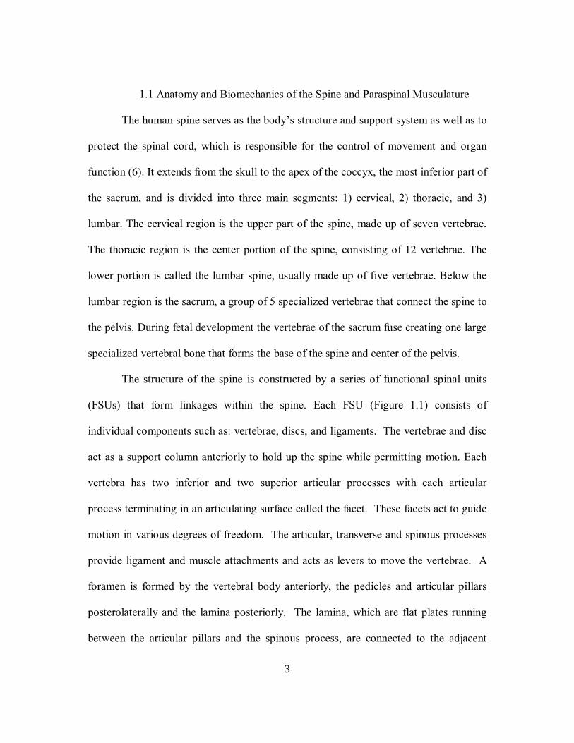
The structure of the spine is constructed by a series of functional spinal units

(FSUs) that form linkages within the spine. Each FSU (Figure 1.1) consists of

individual components such as: vertebrae, discs, and ligaments. The vertebrae and disc

act as a support column anteriorly to hold up the spine while permitting motion. Each

vertebra has two inferior and two superior articular processes with each articular

process terminating in an articulating surface called the facet. These facets act to guide

motion in various degrees of freedom. The articular, transverse and spinous processes

provide ligament and muscle attachments and acts as levers to move the vertebrae. A

foramen is formed by the vertebral body anteriorly, the pedicles and articular pillars

posterolaterally and the lamina posteriorly. The lamina, which are flat plates running

between the articular pillars and the spinous process, are connected to the adjacent

4

vertebrae above and below by the ligmentum flavum. This completes the enclosure of

the canal between the vertebrae posteriorly.

Figure 1.1 Functional spinal unit

The primary purposes of the intervertebral disc is to act both as a shock absorber

and major restraining ligament for the spine. Therefore, its resiliency is said by some to

be responsible for the stability of the spine as a whole (7). The basis of stability is a

point that is much debated by other researchers (8) who state that based on their

material properties, the vertebrae should be attributed as the main source of spinal

stability. Shock absorption allows the spine to compress and rebound pseudoelastically

when the spine is axially loaded and it resists the downward pull of gravity on the head

and trunk during prolonged sitting and standing (7). The structure of the disc is a

complex, composite material that can be classified into two main components: the

nucleus pulposous (NP) and annulus fibrosis. The nucleus is the gelatinous central

portion of the disc and is composed of 80 - 90% water. The solid portion of the nucleus

is primarily Type II collagen and non-aggregated proteoglycans. The annulus is the

outer ligamentous ring around the NP and hydraulically seals the nucleus allowing

intradiscal pressures to rise as the disc is loaded. The annulus has overlapping radial

5

bands, which allow torsional stresses to be distributed under normal loading without

rupture. For this reason, the disc functions as a pressure vessel: as the nucleus is

pressurized, the annular fibers serve to increase stiffness and to prevent the nucleus

from bulging or herniating (7). The gelatinous nuclear material directs the forces of

axial loading radially outward, and the hoops of annular fibers convert disc pressure

into axial force helping to distribute the load without injury (7). Additionally, the

height of a healthy disc maintains the separation distance between the adjacent bony

vertebral bodies. This allows biomechanics of motion to occur, allowing for the total

range of motion of the spine. Proper spacing is also important because it allows the

intervertebral foramen to maintain its height, which in turn allows the segmental nerve

roots room to exit each spinal level without impingement (9).

The lumbar spine is located in the lower portion of the spine and extends from

the thoracic spine to the sacrum. It is responsible for bearing up to 51% of body weight

(10, 31) while permitting forward, backward and side bending as well as rotation by

nature of the kinetic chain of FSUs forming a flexible beam-column. Generally, the

motion of the body is divided between the five segments in the lumbar spine, which

include the L1-2, L2-3, L3-4, L4-5 and L5-S1 levels. The majority of the force caused

by body motion and weight is located at the L4-5 and L5-S1 levels; thus, making these

locations the most likely to be affected by degeneration and instability (6). The normal

spine, as a whole, has an "S"-like curve, which allows for an even distribution of body

weight. The "S" curve helps a healthy spine withstand compressive and shear stress

caused by body motion, e.g. walking, bending and sitting.

6

The single most important mechanical function of the spine is to support loads

that result from the interaction between external loads and muscular tensions while

permitting flexibility. More specifically, the lumbar spine is anatomically close to the

hips causing it to be the primary load bearing section of the spine (10). Fifty percent of

flexion or bending forward occurs at the lumbar region. For this reason, there has been

an increased interest in the mechanics and modeling methods associated with the

lumbar spine, particularly investigating the mechanical properties of the diseased

lumbar disc. Consequently, in-depth static mechanical equilibrium based models have

been developed to give researchers and clinicians alike an improved visualization of the

mechanical interactions as well as the injury mechanics associated with the lumbar disc

and the surrounding muscle tissue. The equilibrium based models are governed by

Newtons Laws of motion. The most prominent of which is the static link segment

model that allows for the determination of lumbar loading conditions (10). Another

commonly used equilibrium approach is the single muscle equivalent model (SEM).

SEMs were created to provide a method for estimating spinal loads in industrial settings

(10) where motions are often repetitious and limited to tasks where simplifying

assumptions can apply. Similar to the SEM, but more anatomically detailed is the

Multimuscle Model, which allows for a better estimate of both the magnitude and

direction of spinal loading (10) under more general movement conditions. Lastly, are

the EMG-Assisted Models (10) that use biological signals to predict muscle tensions

and allow for tensions to be partitioned among muscles according to the recorded EMG

activity.

7

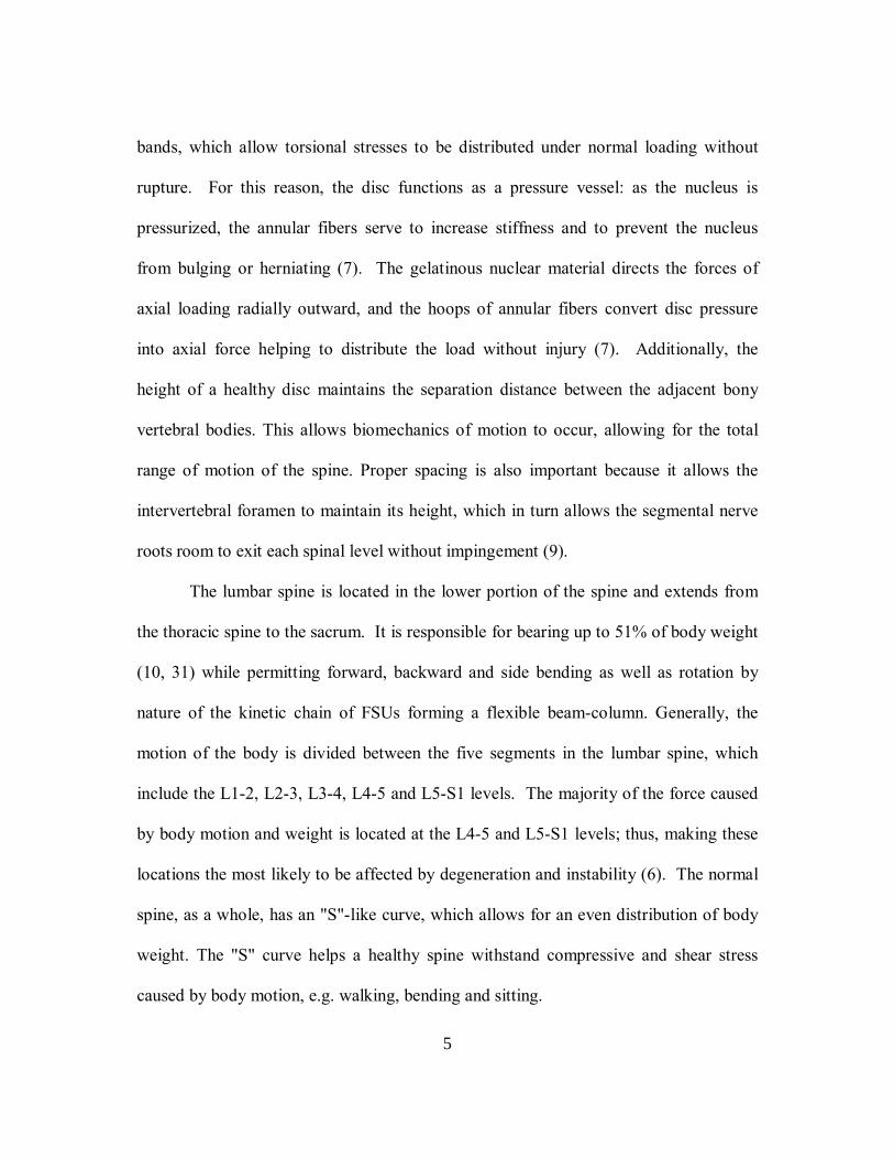
Upon examining a cross-sectional area of the lumbar spine (Fig. 1.2), it can be

seen that numerous muscles surround the spinal column. The group of muscles that are

primarily responsible for the mechanical stability of the spinal column are called the

paraspinal muscles (6).

Figure 1.2 Cross section of the lumbar spine paraspinal muscles (Adapted with permission from Primal Pictures Ltd.)

Typically, an osteoligamentous human lumbar spine can withstand a maximum

compressive load of 90 N before it will buckle (3, 11, 12). The primary role of the

paraspinal muscles is to form a support structure that will stiffen the spine and prevent

buckling (3, 13, 14). The muscles are attached at different levels along the spine and

the tension in the muscle acts to sustain the spine under large compressive forces (3, 13,

14). If a local tension within a muscle is reduced or inadequately timed, the support

system fails causing the spine to be vulnerable under compressive loads.

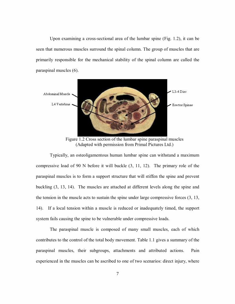
The paraspinal muscle is composed of many small muscles, each of which

contributes to the control of the total body movement. Table 1.1 gives a summary of the

paraspinal muscles, their subgroups, attachments and attributed actions. Pain

experienced in the muscles can be ascribed to one of two scenarios: direct injury, where

8

a muscle is strained or indirect injury related to spasms resulting from an injury in the

spine (6). It has been well documented in the literature (15) that the response of trunk

muscles are delayed in patients experiencing LBP and is indicative of a reflex rather

than voluntary action. Marras et al. demonstrated that there was a change in the muscle

recruitment patterns of LBP patients that increased the loading conditions of the spine

for a longer period of time (11). As such it is hypothesized that the activity of the

muscles, e.g. timing and sequence of recruitment during tasks and or amplitude, may

hold useful information with respect to the nature and/or location of injury to the

structure of the back.

9

Table 1.1 Summary of Paraspinal Muscles

Major Muscle Group Subgroup Origin Insertion Action

Iliocostalis lumborum

Common tendinous origin (same for all lower erector spinae)

Lower border of angles ribs (5) 6-12

Erector Spinae

Longissimus thoracis

Common tendinous origin, sacrum iliac crest, spinous processes of lower thoracic & most lumbar vertebrae

Transverse processes of all thoracic vertebrae, all ribs between tubercles and angles, transverse processes of upper lumbar vertebrae

Bilateral: extension of vertebral column, maintenance of erect posture, stabilization of vertebral column during flexion, acting in contrast to abdominal muscles and the action of gravity. Unilateral: lateral bend to same side rotation to same side opposite muscles contract eccentrically for stabilization

Multifidus lower portion of dorsal sacrum PSIS, deep surface of tendenous origin of erector spinae mamillary processes of all lumbar vertebrae

spinous process of all vertebrae extending from L5 - C2 (skipping 1-3 segments)

Bilaterally extends vertebral column, controls lateral flexion to side opposite contraction (eccentric for stability) unilaterally rotate vertebral bodies (column) to opposite side

Long rotators transverse process of one vertebra

one vertebra to insert on the base of spinous process of vertebra above

Rotate to opposite side, bilateral extension

Transversospinal Muscles

Short rotators transverse process of one vertebra

base of spinous process of vertebra immediately above

Rotate to opposite side bilateral extension

10

Because of the heavy loading conditions frequently undergone by the disc, many

individuals develop low back pain associated with various disc disorders. Of particular

interest in the present study is the pathology of internal disc derangement. Progressive

loss of the water binding capacity and a deterioration of nuclear function causes the

nucleus to be less able and sustain pressure. Because the disc in longer able to bind

water, greater loads are placed on the annulus fibrosus. The annulus is unable to sustain

the load; the disc loses height; and this changes the function of all the joints in the

affected area. Nuclear degradation eventually extends peripherally to affect annular

fibers, typically along radial fissures that have formed, which can lead to disc

protrusion/herniation. Once the disc is torn, it becomes more unstable by allowing for

excessive motion in extension. Figure 1.3a and 1.3b show a CT scan of a healthy and

deranged disc respectively.

(a) (b) Figure 1.3 (a)CT scan of a healthy L5/S1 disc, (b)CT scan of a deranged L5/S1 disc

with an annular tear

11

1.2 Diagnosis of Low Back Pain

Diagnosis of back problems is difficult. In part because of the overlap of

structures, innervation and the commonality of pain patterns, but also because the

relationship between the presence of abnormality including pathology is not direct. As

many as 28% and 85% of the adult male and female population respectively, having no

symptoms or restrictions in activity of daily living are known to have anatomical

pathology in the form of multilevel degeneration or disc bulge (16). Yet they are

functional with no or limited pain experience. Studies suggest that the current

diagnostic techniques have a low degree of sensitivity for findings of disc degeneration

and bulge/herniation as they relate to LBP (16). Magnetic resonance imaging (MRI)

and computed tomographic (CT) scanning have been found to demonstrate

abnormalities in "normal" asymptomatic people (17-19). Positive findings in patients

with back pain therefore have reduced or, at best, questionable clinical significance. In a

study conducted by Jensen et. al., MRI scans revealed herniated discs in approximately

25% of asymptomatic persons less than 60 years of age and in 33% of those more than

60 years of age (18). Clearly, the presence of abnormalities does not correlate well with

clinical symptoms. Common methods currently in use to diagnose back problems

include imaging studies, such as X-ray, MRI and CT scanning, as well as subjective

pain questionnaires and range of motion screening.

12

1.2.1 Imaging Studies

Although there is a broad range of imaging techniques used to diagnose LBP,

the common standards for these diagnostic tests are X-ray, computed tomography (CT),

magnetic resonance imaging (MRI), myelography and discography.

Traditionally, doctors relied on spine x-rays to diagnose patients; however,

literature suggests that there are multiple problems with this approach. The most

prominent of these studies is a 10-year long Swedish investigation that demonstrated

that at least for adults under age 50, X-rays added little diagnostic value to office

examinations, with unexpected results found in only one out of 2,500 patients (20).

Epidemiological research (21-23) showed that many conditions of the spine are often

times unrelated to symptoms and that large numbers of pain-free people have been X-

rayed to reveal that spine abnormalities were as common in asymptomatic people as in

those with pain. Hence, X-rays can be misleading for both the patient and physician

alike. Low-back X-rays involve exposing a patients radiosensitive tissues to large

doses of ionizing radiation, more than 1,000 times greater than that associated with a

chest X-ray; and, the interpretation of the results gained from the test are highly

subjective, which can lead to uncertainty and at times inappropriate treatment (20, 24,

25). The most recent clinical guidelines limit the use of X-rays to specific patients, for

example, those who have suffered major injuries from falling or an automobile accident

(20).

Because X-rays can only be used to view hard bone structures, the diagnoses

like disc protrusions or spinal stenosis requires the use of more advanced imaging

13

technology such as myelography, CT or MRI. Typically patients suspected of having

these disorders and being referred for this type of diagnostic testing are potential

surgical candidates. They present with an appropriate pain syndrome (e.g. radicular leg

pain, nerve root irritation and limited straight leg raising) or are patients suffering

chronic LBP, who have had a poor response to 4 to 6 weeks of conservative therapy and

require a more definitive diagnosis (20). Myelography uses static X-ray or fluoroscopy

to provide pictures of the cavity within the spinal canal that has been injected with a

radiopaque dye. Myelography may be done to detect blockage of the spinal canal

caused by a tumor, infection, a herniated disc, or arthritis. A computed tomography

(CT) scan uses X-rays to produce detailed pictures of structures inside the body. A CT

scanner directs a series of X-ray pulses through the body that lasts only a fraction of a

second and represents a slice of the organ or area being studied. A dye that contains

iodine (contrast material) that makes blood vessels and other structures or organs more

visible is often injected into the blood during a CT scan. The dye may be used to

evaluate blood flow, detect tumors, and locate areas of inflammation. MRI is a test that

can provide a detailed picture of structures and organs inside the body. It uses a

powerful magnetic field and radio signals to create the picture. Often times MRI

provides more detail than other tests, such as a CT scan, and does not require X-rays or

the injection of dyes or other substances. It may be used to create images of joints,

including the joints of the spine where it can detect problems such as joint injuries or

herniated discs. MRI is most effective at providing pictures of tissues or organs that

contain water but is not as useful for looking at structures that do not contain water.

14

Both myelography and CT scanning show herniation/protrusions in approximately 20%

of persons who have never had back pain (20). Similarly, MRIs show herniations in

almost 10% of asymptomatic young women and bulging discs in 45% (26). Without

the patient having significant clinical findings of LBP, these results will frequently lead

to ill-advised diagnoses that can cause a string of invasive clinical interventions,

especially when these imaging studies are done too early or in the absence of surgical

indications (20). The sensitivity and specificity of these imaging studies also appears to

be inefficient. It has been shown that CT and myelography have a sensitivity level of

80-90% but specificity as low as 68% in the diagnosis of herniated lumbar discs (27).

Another imaging study that remains controversial is lumbar discography (20).

This study is generally conducted when X-rays and MRIs do not yield specificity as to

the disc causing the clinical symptoms (28). In this method a radiographic contrast is

injected into the nucleus of each disc to be investigated. While the CT image taken of

each disc assists in the diagnosis, a key component of this test is the pain provocation, if

any, that can be compared to the patient's clinical pain. For this reason, there are three

outcomes that can result from a discogram procedure: two types of negative, and one

positive. A negative test may result from a normal CT or an abnormal CT scan but

failure to reproduce the patient's clinical symptoms. A positive test is noted when the

CT scan shows abnormality associated with reproduction of a patient's clinical

symptoms (28). Typically, the discogram is used specifically for determining if disc

degeneration causes pain without a herniation or nerve root compression. A positive

discogram has been said to be indicative of the need for a spinal fusion, a surgical

15

technique in which one or more of the vertebrae of the spine are fused together so that

motion no longer occurs between them. However, it has been argued that the value of

the discogram result does not compensate for the high subjectivity, invasiveness and

technical demand of the study (20). According to a study conducted by Deyo et. al.,

discography can identify internal disc disruption in approximately 40% of patients (20).

Table 1.2 summarizes the lumbar spine imaging procedures used clinically (20).

Table 1.2 Lumbar Spine Imaging Procedures in Clinical Use

1.2.2 Functional Measurement Studies

An alternative approach to imaging is that of functional measurement. There are

a number of options where the technical instrumentation already exists and is well

Procedure Methods Utility Plain Radiography Multiple Views View spinal vertebrae, able to

detect degeneration

Computed Tomography

Plain Computed Tomography Computed tomographic myelography Computed tomography with 3-dimensional reconstruction

Used for conditions that only affect the bones of the spine

Myelography X-ray with contrast material Investigate shape of the spinal sac and to determine if there is pressure on the nerves

Magnetic Resonance Imaging

Magnetic waves, picture slices of the spine with 3-diMESional reconstruction

Allows view of both hard a soft tissues in the spine

Discography CT scan with contrast material

Test for disc abnormalities and concordant pain conditions. Used for determining specificity of LBP.

16

understood. This includes objective measures of range of motion (ROM) and strength as

well as subjective self-reported patient questionnaires.

ROM is defined as the maximum angular deviation of a given joint and is used

to classify joint motion or mobility. One of the clinical aspects of LBP impairment is

decreased vertebral mobility and strength. The gold standard for spinal ROM is the

double inclinometer (DI) method (30). The DI method is based on the constant effects

of joint to orient the inclinometer and offers the possibility of excluding the hip range of

motion form the total flexion of a patient during bending. The relative motion measured

between the T12 level and the sacrum is used to represent lumbar spine motion. The

major drawbacks to this method are that the patient must remain in the flexion position

long enough for the clinician to read both inclinometers, which can cause a greater level

of discomfort and it is prone to measurement error from a number of sources. Thus, the

clinical use of this method is unpopular because it requires a moderate amount of skill

and training and is time-consuming (30). There are many factors that effect range of

motion data, including: age, gender, body stature, body weight and patient apprehension

of movement. Typically, after the 10- to 16-year age group, joint motion decreases by

about 10% from that of the first decade (31). However, studies have shown that gender

plays a significant role in the increase in joint mobility from men to women, with

women having a more than 100% increase in joint mobility versus men.

To allow clinicians to gain an understanding of the patients perspective of their

pain, self-reported patient questionnaires have increasingly become the standard method

17

of evaluation for patients with low back pain. Patients suffering from chronic LBP

typically report psychological distress and functional impairment, which they often

attribute to the severity of their pain (32, 33). Utilizing a screening tool can alert

clinicians to the presence of such distress and potentially leads to improved treatment

outcomes and reduction of patients long-term disability (32, 33). There are a number

of measures currently available, including but not limited to: the Oswestery Low Back

Pain Disability Index (ODI), the Visual Analog Scale (VAS) and the SF-36.

The most familiar of these questionnaires is the ODI, which was developed by

John O Brien, a specialist working with patients with chronic low back pain. The ODI

questionnaire was designed to identify the changes in the daily activities of patients due

to LBP (34, 35). The test is self-administered, which enhances its utility and has been

shown to have high test-retest reliability as well as having been validated in numerous

low back pain studies (34). It consists of ten items, with questions ranging from pain

intensity to personal care and social life effects.

The VAS is designed to present to the patient a rating scale with minimum

constraints. Patients mark a location on the line corresponding to the severity of pain

they experience allowing them the greatest freedom to choose the exact intensity of

their pain. Several versions exist, each giving a different level of precision in the

estimate. Test-retest reliability has been shown to be good (24, 36-38).

The SF-36 was designed for use in clinical practice and research, health policy

evaluations, and general population surveys in effort to quantify the patients perception

of their quality of life. The SF-36 includes one multi-item scale that assesses eight

18

health concepts: 1) limitations in physical activities because of health problems; 2)

limitations in social activities because of physical or emotional problems; 3) limitations

in usual role activities because of physical health problems; 4) bodily pain; 5) general

mental health (psychological distress and well-being); 6) limitations in usual role

activities because of emotional problems; 7) vitality (energy and fatigue); and 8) general

health perceptions (39).

Although, the use of questionnaires are acceptable for the average patient

population, patients who have severe disc related or chronic pain often have additional

psychosocial factors affecting ROM data and surveys, including but not limited to:

subject intent, willingness to perform, and fear of activity related pain. Studies (40-44)

have shown that performance of patients with lumbar pathology can be affected by

psychological factors, which cause them not to give an accurate portrayal of their ROM,

muscle strength, ability to perform daily activities and report increases in their

perceived pain intensity.

1.3 Electromyography

In contrast to anatomic imaging and other noninvasive functional measures, e.g.

range of motion and strength testing, surface electromyography (sEMG), evaluates the

physiological functioning of the back muscles that may be less influenced by subject

intent or willingness to perform (45, 46). Measures such as ROM and strength evaluate

a patients ability to perform certain movements such as lateral bending,

flexion/extension and straight leg raise for ROM or knee extension and plantar flexion

power for muscle strength tests. The pitfall of these tests is that they are influenced by

19

self-efficacy beliefs, i.e. the patients belief in their physical capacity (40, 47). Pain-

related fear of physical activity causes avoidance of activity and higher disability (40,

47). sEMG, a noninvasive objective measure, records the summation of activity from

muscle groups within the recording area under the electrodes. As the bioelectric

potentials reach the skin surface through volume conduction, electrical currents spread

(are conducted) three dimensionally through the volume of the body segments. Because

of the conductivity of tissue, at rest the volume conductor formed by the body is of

equal potential (isopotential) at all points. When a dipole is formed, current flows until

the point of isopotential is reached (45). Because sEMG relies on the placement of the

electrode, the amplitude of the waveform seen will be at its maximum when the

electrodes are aligned with the line of contraction of the muscle.

Muscle activity, while it may be influenced by other factors including, subject

intent, emotion, and reflex response, is driven from a biomechanical perspective largely

by postural task (29, 48-51). Because the sEMG potentials are driven primarily by the

necessity to maintain trunk stability and rigidity in response to a specified task, it tends

to be more objective. That is, the muscular recruitment is less likely to be altered

significantly by volitionally altered control. sEMG differs from needle

electromyography (nEMG) in that nEMG quantifies the summated action potential of

small regions of muscle. Needle insertion into the muscle evokes a bursting of fiber

activity that reflects the sensitivity of the membranes. Intact neural control of the

muscle fibers influences that sensitivity. As a result, nEMG can be used to represent not

only aspects of the muscle health but also that of its innervation. nEMG has the

20

advantage of being used to determine the presence and location of disease or injury to

the nerve or muscle itself. At the same time it has several disadvantages. The nEMG is

able to record activity from subsections of individual muscles but, it is not able to

adequately represent the extent of muscle activation as a whole. Most back pain patients

do not have disease affecting the nerve or muscle directly. Finally, nEMG is a painful

invasive procedure with some small risks of injury or infection.

Paraspinal surface EMG, has been evaluated as a means to identify myoelectric

signal patterns of recruitment timing and intensity as they relate to specific tasks. These

methods have been used in muscles of the extremities and in the paraspinal muscles for

healthy subjects and patients with back pain. Measurement strategies include use of a

single electrode pair overlying a target muscle or an array of electrodes placed on the

skin surface. Recordings are made either at rest, under loading from various postures or

tasks and, after a series of exercises. Electrical activity of the muscles has been

represented in various ways including simple pattern descriptions, envelope integration

amplitudes, epoch RMS values and frequency power spectra (52).

1.4 Previous Work

In the past there have been numerous studies aimed at understanding the

behavior of the paraspinal muscles in low back pain patients. Two primary approaches

can be identified. The first involves the monitoring of patterns and amplitudes of

myoelectric activation during designated tasks. One of the earliest findings was reported

in the 1950s with the definition of a phenomenon called flexion-relaxation (FR). FR is

measured from the paraspinal musculature of the low back during forward flexion tasks.

21

FR, defined by Allen, is the change in EMG activity of the paraspinal muscles

occurring as a person bends forward from standing (53). Typically for normal

subjects, the EMG activity increases as the load increases and the muscles support the

spine; then, as the ligaments take over, the muscles relax to a level below that of the

standing EMG activity. Triano and Schultz were among the first to show that the

presence or absence of FR was related to patient reported disability (38). They found

that healthy controls subjects had three clearly separate phases of back muscle

activation: 1) bending forward, 2) fully flexed and 3) rising to stance. In contrast,

subjects who had high Oswestry test scores showed a loss of flexion relaxation and hat

the three phases of FR were no longer apparent (Figure 1.4) (38). In Figure 1.4a, the

behavior of the paraspinal muscles, both left (top) and right (bottom), during a cycle of

forward flexion and recovery is shown. The cycle begins with a subject in upright

standing position (a). As the subject initiates trunk flexion, myoelectric activity appears

as a result of eccentric contraction in the lumbar paraspinal muscles to provide a

controlled lowering of body mass (b). At approximately 45° of flexion, the electrical

signal spontaneously diminishes (c) reflecting cessation of movement within the lumbar

spine and transfer of motion to the pelvis and hip joints. On recovery from full flexion,

the electrical signal remains silent at the initiation of trunk extension (d). As the

pelvic/hip function completes the initial recovery, then muscles become even more

active reflecting the need to oppose gravitational influence as the upper body returns to

upright position (e). In contrast, Figure 1.4b shows the same stages of flexion

movement for a subject with LBP. The FR phenomena is absent and asymmetric

22

myoelectric response appears during this sagitally symmetric task. Overall, Triano and

Schultz concluded that myoelectric signal levels may be objective indicators of low

back pain disability.

(a)

(b)

Figure 1.4 (a) Left (blue) and right (green) paraspinal muscle activity of a pain free subject during a flexion task (b) Left (blue) and right (green) paraspinal muscle activity

of a LBP patient during a flexion task

Subsequent studies (38, 49, 54-63) have examined reproducibility, consistency and

responsiveness to treatment. Results found in these studies were inconsistent at best and

23

in many cases, have been conflicting. Most of the conflict resulting from the method

used to establish the presence or absence of the FR phenomena, e.g. Mathieu and Forin

suggested that FR is present if muscle activity during full flexion is less than 10% of

muscle activity during re-extension and Haig et al. determined that the subject had

reached FR if EMG levels were greater standing than when fully flexed (64). Paquet et

al calculated a ratio between EMG at full flexion divided by EMG at midflexion, and

found that 40% of the chronic LBP patients tested exhibited the FR state (64). A

consistent feature however, is that they all clearly establish that normal flexion-

relaxation is biomechanically constrained. Although FR may be affected by functional

and or pathological states, it cannot determine or discriminate between them.

In conjunction with the FR technique, is pattern recognition of the muscle

activity. A number of authors have attempted to relate changes in muscular recruitment

patterns to the presence of pain (55, 78, 79, 91-97). Price et al was one of the first to

correlate a patients pain to the level of activity in an EMG. He found that paraspinal

EMG patterns tend to be asymmetrical with respect to bilaterally symmetrical

movements such as flexion (98, 99). Price observed patterns of muscle behavior that he

could assign to qualitatively different groups. Descriptive attributes for LBP patients

included: 1) asymmetrical activity in movements where bilateral symmetry was

expected, 2) characteristic overactivity, and 3) characteristic underactivity of a region

when compared to the pain free control subjects (98, 99). The authors hypothesized that

the hyperactiviy could be explained by reflex spasm due to pain or as a method for

24

avoiding contraction of another muscle that would result in pain (98, 99). Conversely,

hypoactivity was explained as a result of reflex inhibition (98, 99).

Janda and Wolf reported similar unexpected bilateral EMG activity, called co-

contraction, during asymmetrical tasks in separate studies (100, 101). These studies

demonstrated that pain free controls showed significantly greater activity in the muscle

contralateral to the direction of movement, whereas low back pain patients did not

display unilateral activity that were markedly different (100, 101). Edgerton et al.

characterized changes in muscle recruitment patterns proposing them as being a result

of muscle dysfunction (102). He found that tissue damage, even in the absence of pain,

can cause a loss of force generating capability and result in neural adaptations with

chronic hypoactive EMG activity patterns (102). Nouwen et. al. attempted to repeat

earlier studies conducted by Janda and Wolf, but failed to establish any statistical

significance for the paraspinal muscle activation intensity and low back pain subjects

(98). The authors postulated that absence of statistical differences arose from the

interaction of the left and right paraspinal EMG activity during dynamic movements.

They proposed that the differences might become more prominent during static

postures, a fact that is supported by the work of Collins et al (103). Collins found that

there were marked absolute left-right differences in paraspinal EMG activity during

exertive tasks, e.g. maximum forward bend (45°) and forward pelvic tilt (103).

A second technique has been to examine the fatigue behavior of muscle under

prescribed conditions where reproducibility and responsiveness have been evaluated

(47, 65-90). Muscular fatigue rates have been shown to change with task duration,

25

repetition and with chronic low back pain. The fatigue technique requires the

determination of a subjects maximal voluntary contraction (MVC) and then recording

the sEMG of the subject at typically 80% MVC for a length of time that would fatigue

the muscle (30-45 sec) (47, 68, 69). The median frequency (f) of the power spectrum is

then calculated for each 1 s interval of the recorded signal and compared to the f for the

recovery contractions where the subject exerts 80% MVC for a controlled amount of

time (5 sec, repeated at standardized time increments e.g. 1, 2, 3 and 5 minutes

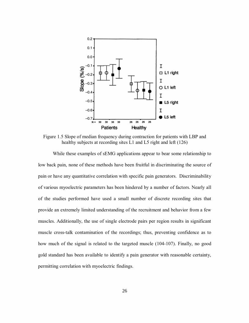
following the fatigue contraction) (47, 68, 69). Dedering et al. found that subjects

having low back pain had on average significantly higher f at L5 than at L1 and

therefore differed significantly from the healthy subjects (126). The fatigue contraction

was analyzed with linear regression analysis of f as a function of time t, from t=0 to

t=45 s (126). For each recording the initial median frequency (fi) was defined as the

intercept at t=0 (126). The decrease of f in slope (%/s) was defined as the slope of the

regression line (Hz/s) divided by fi/100 (126). Slopes which were significantly negative

were considered fatigue present and slopes not significantly negative as fatigue absent

(126). As Figure 1.5 shows, the LBP patients had on average significantly flatter slopes

(%/s) than healthy subjects (126). Overall, they found that significantly more patients

(58%) than healthy subjects (36%), i.e. had no EMG fatigue, i.e. 24 sites without

significantly negative slopes (126). In contrast to the pattern recognition studies, they

found no significant left-right difference between LBP patients and healthy control

subjects (126). Further, it still remains unclear as to what the source of pain may be.

26

Figure 1.5 Slope of median frequency during contraction for patients with LBP and healthy subjects at recording sites L1 and L5 right and left (126)

While these examples of sEMG applications appear to bear some relationship to

low back pain, none of these methods have been fruitful in discriminating the source of

pain or have any quantitative correlation with specific pain generators. Discriminability

of various myoelectric parameters has been hindered by a number of factors. Nearly all

of the studies performed have used a small number of discrete recording sites that

provide an extremely limited understanding of the recruitment and behavior from a few

muscles. Additionally, the use of single electrode pairs per region results in significant

muscle cross-talk contamination of the recordings; thus, preventing confidence as to

how much of the signal is related to the targeted muscle (104-107). Finally, no good

gold standard has been available to identify a pain generator with reasonable certainty,

permitting correlation with myoelectric findings.

27

1.5 LASE Monitoring

The LASE technology represents a new approach to monitoring back muscle

behavior. Its application may impart a potential solution to several of the problems of

earlier approaches. The electrode array provides a comprehensive sampling of muscle

activity of the lumbar region using 206 pairs (plus 1 ground) of electrodes to map the

regional muscle behavior. The parallel principle, which states that the muscles aligned

with the electrode pair parallel to its line of contraction are the muscles contributing the

largest proportion of amplitude observed in the waveform, is invoked in effort to

identify the likely muscle source for the majority of the activity observed by a pair of

electrodes. Through graphical overlay (Figure 1.6) comparisons with the location and

orientation of back muscles that might be contributing to the sEMG signal (108) are

made. The analysis software permits selective comparisons of electrode pairs,

graphically overlayed with the underlying anatomy, so that most parallel muscle to the

myoelectric activity can be estimated by use of the parallel principle. Moreover, access

to the actual signal from each electrode allows for an innovative analyses and lends

itself to cross-talk nullification (106) and pattern recognition through intelligent

algorithms such as neural network modeling (109).

28

Figure 1.6 LASE graphical representation of the myoelectric grid overlayed on a layer of back muscles. The circle represents an example of a local electrode and its neighbors

used to evaluate the relative activation and its trajectory

In a single study, myoelectric patterns observed from the LASE array during

standardized testing have been shown to discriminate patients with lumbar facet joint

inflammation through subjective pattern identification. Comparing muscle activity

during standardized tasks, changes in patterns of back muscle recruitment and pain

relief were contrasted before and after therapeutic facet injection. These patterns were

compared again with those from a population of patients having pain and internal disc

derangement determined from abnormal CT discography (110). Finneran et al. also

sought to characterize the response patterns of the paraspinal muscles of subjects

following an episode of acute LBP. In this study he determined that the LASE system

could be used to classify the severity of acute LBP and identified four response-pattern

subgroups: 1) normal low back response with symmetrical images, 2) acute LBP images

29

that were asymmetrical 3) acute LBP images that had multiple foci and 4) acute LBP

images that were both asymmetrical and mutifocal (111). However, it remains to be

determined whether the observations by Finneran et al. can be represented

quantitatively to discriminate between healthy and low back patients. Similarly, it is

unclear whether specific pain generators engender quantifiable differences based on

tissue of origin. Such a quantitative measure would provide an objective means that

could be more generizable for evaluating back pain patients.

1.6 Hypotheses and Specific Aims

The primary purpose of the present work was to evaluate the hypothesis that the

quantitative description of symmetry/eccentricity of regional low back myoelectric

behavior would be significantly different for healthy patients versus those with probable

discogenic low back pain during standardized tasks. A secondary purpose was to

quantitatively compare the predicted muscle loading of the spine from myoelectric

activation in patients and healthy subjects performing the same tasks using a first-order

approximation. To achieve testing of these hypotheses, several specific aims were

created to stage their development, validation and implementation.

! Specific Aim 1: Develop a simple sagittal plane, single muscle equivalent,

lumped parameter RMS-MES (root mean square-myoelectric signal) regression

model that estimates the muscle activity contribution to spine compression loads

under standardized tasks.

! Specific Aim 2: Validate the biomechanical model through comparison with

3DSSP U of M model.

30

! Specific Aim 3: Test myoelectric behavior from homogeneous sample

populations of healthy and discogenic low back pain subjects performing a

series of three standardized static postural tasks designed to induce

monotonically increasing spinal loads.

! Specific Aim 4: Develop simple regression models to predict the component of

spinal loads contributed from myoelectric activation, testing for differences

between healthy and discogenic low back pain.

! Specific Aim 5: Quantitatively define the differences in symmetry/eccentricity

of regional myoelectric behavior between groups using RMS-MES differences

between electrodes and their vectorial locations with respect to a common

reference site.

! Specific Aim 6: Apply step-wise regression analysis to identify any parameters

important to discriminating behavior differences between healthy and discogenic

low back pain patients.

31

CHAPTER 2

METHODS

2.1 Instrumentation

The Large-Array Surface Electromyographic (LASE) Imaging System used in

this study was developed by the Paraspinal Diagnostic Corporation in Columbus, Ohio.

The Food and Drug Administration has cleared this device for clinical use to monitor

and display the bioelectric signals produced by muscles to aid in the diagnosis and

prognosis of muscular disease or dysfunction (110-112).

The LASE system uses a 18 cm x 23 cm array of 63 adhesive surface electrodes,

each 2.5 cm apart, integrated into a flexible sheet (Figure 2.1). The central electrode is

the reference electrode and the remaining 62 electrodes are related to this electrode. A

grounding strap is placed on the subjects wrist. Using standardized skeletal landmarks

(reference electrode placed over the L3-4 disc); the array is applied to the subjects low

back overlying the lumbar spine and paraspinal muscles so that it is consistently located

and scalable with respect to underlying muscles.

32

Figure 2.1 LASE flexible electrode array

Table 2.1 gives a detailed listing of the specifications for the LASE instrumentation.

Table 2.1 LASE Specifications Specification Description

Operating System Windows NT, Pentium II, 64 channel A/D converter (Paraspinal Diagnostic

Corporation in Columbus, Ohio ) Sampling Rate (frequency) 2 kSamples/sec

Sampling Capacity 500 kSamples/sec Lowpass Filter (corner frequency) 500 Hz +/- 5% Highpass Filter (corner frequency) 1 Hz +/- 5%

Common Mode Rejection Ratio @ 60 Hz (per channel) 80 dB

Input Impedence >10,000 MW //2pF Output Impedence 200 W

Differential Mode Gain (per channel) 88.0 +/- 0.5% Supply Voltage 120 V

Input Bias Current 100 pA @ 25º C A/D Resolution 1.2 mV

The sEMG is calibrated to individual stature by anthropometric (subject height and

weight) as well as topographical measures, e.g. spine length (distance from the lower

scapula to L-4) and lateral distance from the L-4 spinous process to the left illium,

Reference Electrode

33

which are obtained prior to sEMG testing. The proprietary software uses these

measures to scale the location of the RMS-MES values recorded by stature such that

comparisons across subjects can be made. Bipolar, differential recordings from the 206

combinations of adjacent electrode pairs are collected over a one second interval, with

an analog-to-digital sampling rate of 2 kHz. The electromyographic activity between

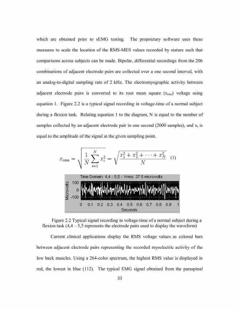
adjacent electrode pairs is converted to its root mean square (xrms) voltage using

equation 1. Figure 2.2 is a typical signal recording in voltage-time of a normal subject

during a flexion task. Relating equation 1 to the diagram, N is equal to the number of

samples collected by an adjacent electrode pair in one second (2000 samples), and xi is

equal to the amplitude of the signal at the given sampling point.

(1)

Figure 2.2 Typical signal recording in voltage-time of a normal subject during a flexion task (4,4 5,5 represents the electrode pairs used to display the waveform)

Current clinical applications display the RMS voltage values as colored bars

between adjacent electrode pairs representing the recorded myoelectric activity of the

low back muscles. Using a 264-color spectrum, the highest RMS value is displayed in

red, the lowest in blue (112). The typical EMG signal obtained from the paraspinal

34

musculature has frequencies that range from 30 to 150 Hz (113, 127, 128). The

sampling rate of the LASE A/D converter is 2000 samples per second per electrode

pair. This sampling rate produces a frequency resolution accurate up to 500 Hz (108),

which is well above the myoelectric frequencies of interest. The MES is amplified

with a gain of 1000 and filtered using both a high (30 Hz) and low (150 Hz) bandpass

filter before being converted by an analog-to-digital converter and stored in data files

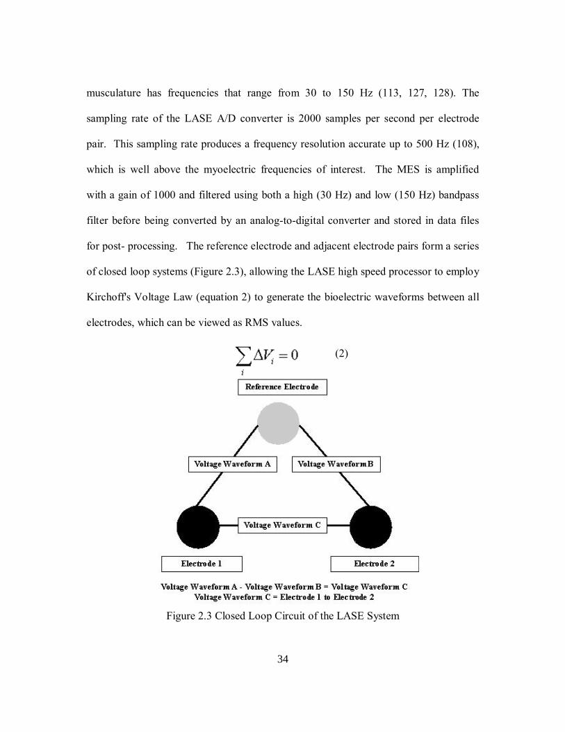
for post- processing. The reference electrode and adjacent electrode pairs form a series

of closed loop systems (Figure 2.3), allowing the LASE high speed processor to employ

Kirchoff's Voltage Law (equation 2) to generate the bioelectric waveforms between all

electrodes, which can be viewed as RMS values.

Figure 2.3 Closed Loop Circuit of the LASE System

(2)

35

As applied here, Kirchoffs law can be defined as the comparison of the waveform

voltage of one electrode, relative to the reference electrode, as subtracted from the

waveform of a second electrode relative to the reference electrode. The difference

between the two waveforms is the signal that would be observed between just those two

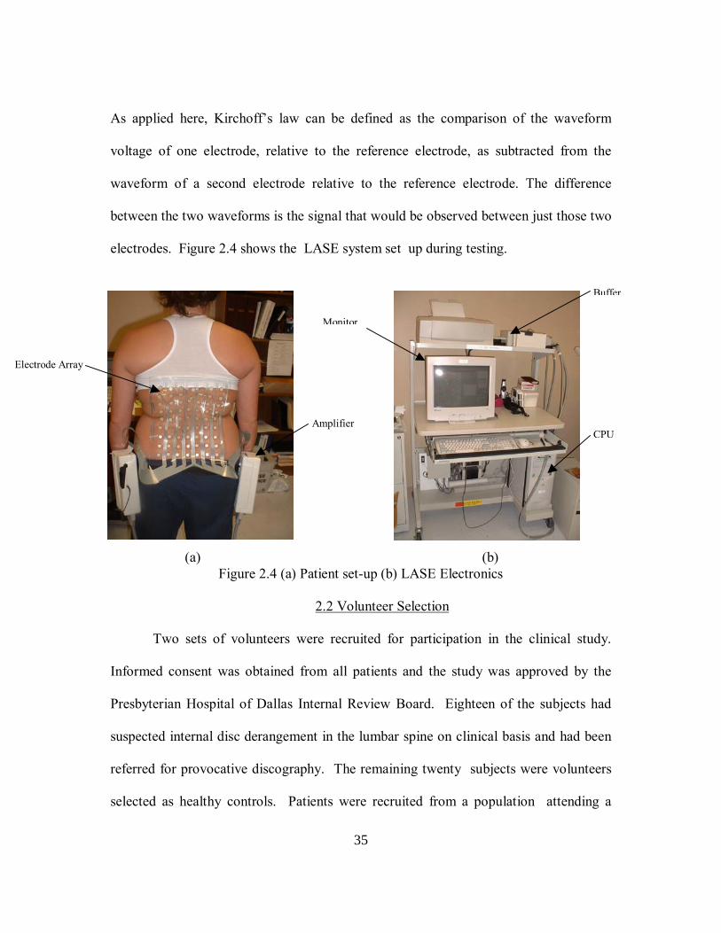
electrodes. Figure 2.4 shows the LASE system set up during testing.

(a) (b) Figure 2.4 (a) Patient set-up (b) LASE Electronics

2.2 Volunteer Selection

Two sets of volunteers were recruited for participation in the clinical study.

Informed consent was obtained from all patients and the study was approved by the

Presbyterian Hospital of Dallas Internal Review Board. Eighteen of the subjects had

suspected internal disc derangement in the lumbar spine on clinical basis and had been

referred for provocative discography. The remaining twenty subjects were volunteers

selected as healthy controls. Patients were recruited from a population attending a

Electrode Array

Amplifier

Buffer

Monitor

CPU

36

clinic for evaluation and treatment of low back pain and restricted to lumbar related

pain. Control subjects were recruited as volunteers who had no history of disabling

low back pain before testing. Volunteers from either group with clinical evidence of

scoliosis were excluded. Subjects in the LBP group had sEMG assessments conducted

prior to having the lumbar discogram. Following the discography, results were

reviewed by a radiologist and copies of the diagnosis were added to the patients study

records. Table 2.2 summarizes the inclusion and exclusion criteria that were used for

each group.

Table 2.2 Summary of inclusion and exclusion criteria for study volunteers

Healthy Controls LBP

Inclusion

! Age 18 - 67 ! No spinal deformity ! No prior spine surgery ! No history of disabling

back or leg pain. ! No history of back pain

for the past 6 months

! Age 18 67 ! Prior spine surgery limited to a

one level laminectomy/discectomy with no instrumentation.

! VAS > 3.0 ! The patient has been referred for

provocative discogram diagnostic study with a suspected single level internal disc derangement.

! Normal psychometric screening.

Exclusion ! Scoliosis ! Progressive neurological deficit

! Scoliosis

2.3 EMG Data Collection

Anthropometric data (height, weight, and age) and torso segment measures

(spine length, lateral and anterior-posterior for both abdomen and thoracic) as well as

subjects body mass index (BMI). The VAS pain scale was completed by each patient

37

to provide a subjective rating of the patients perceived level of pain. The subjects spine

length and transverse thoracic diameter (at T7) were obtained to scale the stature of the

subject in the LASE interface.

After the subjects skin surface was treated with isopropyl alcohol to remove

any residue that would impede the electrical signal. Unprepared skin resistance can be

2MΩ or greater except when wet or with perspiration (113). Skin impedance is reduced

to <10KΩ by using isopropyl alcohol, which also dries out the skin, providing

insulation from static electricity (113). The electrode array was applied as shown in

Figure 2.4a. Myoelectric data was collected during three postural tasks (Figure 2.5):

upright (Figure 2.5a), forward flexion (Figure 2.5b, bent 20º at the hip) and weighted

(Figure 2.5c, subject stands upright with arms stretched out and holding 5 lb weights in

each hand).

(a) (b) (c) Figure 2.5 Standardized Postures Used During EMG Testing: (a) Upright,

(b) 20° Lumbar Flexion, (c) Weighted

38

Subjects began testing in an upright stance then, the sequence of testing progressively

increased the demand on the musculature of the lower back to offset postural loads (31).

The tasks selected were those reported in the literature to be associated with negligible

abdominal muscle recruitment and only sagittally symmetric flexion moments acting on

the spine (110, 111). The flexed posture task was determined by inclinometer measure

taken at the L4/L5 landmark. Each position was held for 1 second during MES

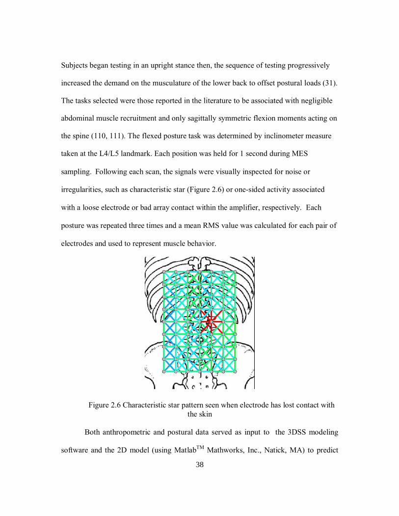
sampling. Following each scan, the signals were visually inspected for noise or

irregularities, such as characteristic star (Figure 2.6) or one-sided activity associated

with a loose electrode or bad array contact within the amplifier, respectively. Each

posture was repeated three times and a mean RMS value was calculated for each pair of

electrodes and used to represent muscle behavior.

Figure 2.6 Characteristic star pattern seen when electrode has lost contact with the skin

Both anthropometric and postural data served as input to the 3DSS modeling

software and the 2D model (using MatlabTM Mathworks, Inc., Natick, MA) to predict

39

the both the passive and active force and moment contributions acting at the level of

L5/S1. Finally, a linear regression model was developed to correlate the RMS data to

the active muscle tension contribution to the total loads.

2.4 Biomechanical Modeling

Direct measurements of the spine forces and moments generated by the

paraspinal muscle would be a highly invasive and risky procedure. Reliable estimates

of spinal loads can be made from appropriately designed biomechanical models (9, 11,

29, 114-119). Models may be simple or complex, depending on their application. For

the purposes of this work to estimate spinal loads during simple static and sagitally

symmetric task, a sagittal plane, single muscle equivalent, lumped parameter

biomechanical model was developed to gain insight into the low back loads and how

they may be generated. Currently, the greatest limitation to modeling the lumbar spine

is the complexity of the back muscles themselves (120). Muscles control movements

and postures, such as flexion, as well s static and dynamic spine stability. At the same

time, the muscle action contributes additional compressive and shear loads on the

lumbar spine in their own right. Consequently the total load acting on the FSU

corresponds to the algebraic sum of the externally applied load from body segment

mass, postural configuration, extrinsic loading and muscle tension (29, 120). The

magnitudes of the active muscle tensions are critical elements in any comprehensive

model that attempts to evaluate the total force exerted on the spine as they can be

significantly large in comparison to the body mass.

40

Loads acting on the spine can be partitioned into active and passive components

(9). Passive forces arise from the upper body mass, and any weight being held in the

hands, acting at the L5-S1 disc level . The passive forces were analyzed using a two

dimensional static model for the sagittally symmetric tasks and hand loads using a

multisegment spine model with reference system at the L5-S1 disc. Free body diagrams

were constructed for each subject performing the three postural tasks: upright, 20

degrees of lumbar flexion and weighted. Figures 2.7, 2.8, and 2.9 are the general

diagrams used to model the forces and moments acting at each disc level.

ΣF = 0: FR = FUB (3)

FL5-S1 = FRcos θ (4) θ = 40°

ΣM=0: ML5-S1 = rUBFUB ≈ 0 (5) rUB<<1

Figure 2.7 Diagramatic Representation of the Upright Posture

41

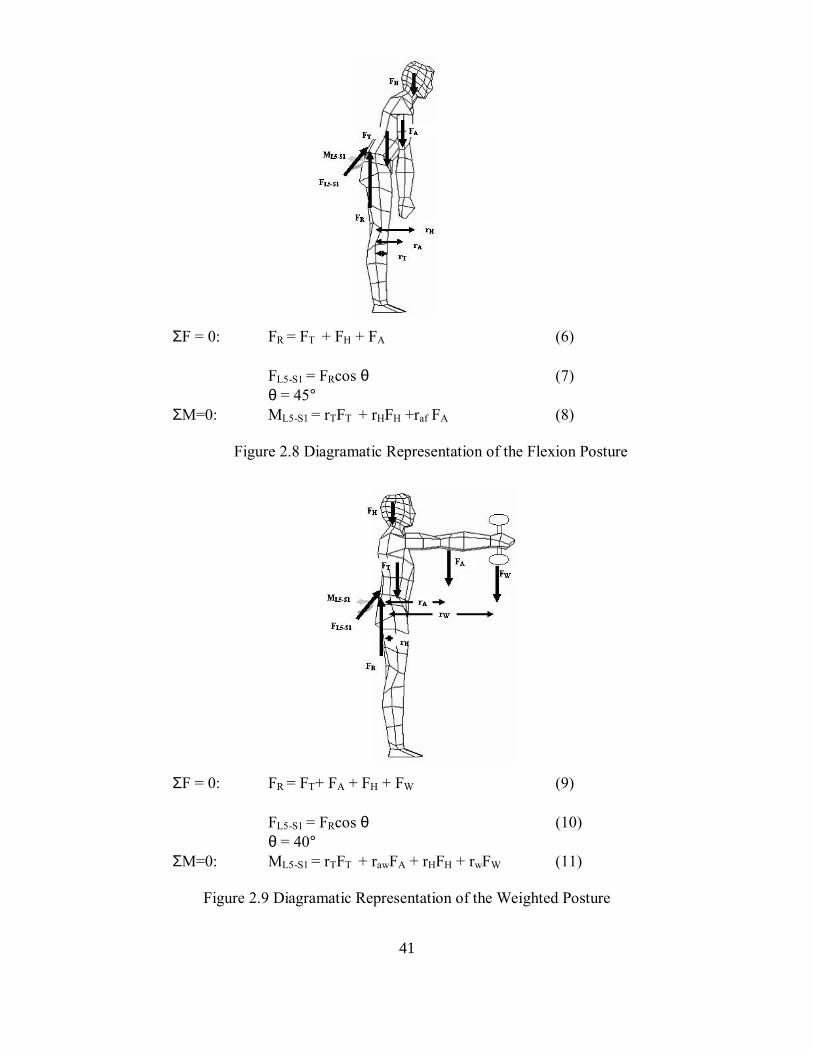
ΣF = 0: FR = FT + FH + FA (6)

FL5-S1 = FRcos θ (7) θ = 45°

ΣM=0: ML5-S1 = rTFT + rHFH +raf FA (8)

Figure 2.8 Diagramatic Representation of the Flexion Posture

ΣF = 0: FR = FT+ FA + FH + FW (9)

FL5-S1 = FRcos θ (10) θ = 40°

ΣM=0: ML5-S1 = rTFT + rawFA + rHFH + rwFW (11)

Figure 2.9 Diagramatic Representation of the Weighted Posture

42

The equations (Eqn. 6-8) that were used for the flexion calculations were similar

to those of the upright (Eqn. 3-5) and weighted (Eqn. 9-11) postures except that the

angle of the joints had to be adjusted for posture (the 20 degrees of lumbar flexion) and

external load (5 lb weight holding). FUB for the upright posture (Figure 2.7) is

representative of the total upper body weight including the trunk, arms and head. FT, FA,

and FH are the trunk, arm, and head loads respectively (Figures 2.8 and 2.9). FW is the

force resulting from the weight being held in the hands (Figure 2.9). Based on the

literature (29, 120, 121), the L5-S1 joint accounts for 25% of the total flexion in

forward bending posture. Therefore, the angle of the joint was taken to be the original

angle of 40 degrees plus an additional 5 degrees attributed to the flexion stance (25% x

20 degrees), for a total of 45 degrees (29, 120, 121). The active component arises from

the muscle tension required to maintain postural equilibrium, imposing additional

compression, shear and moment loads on the disc. The line of action of the erector

spinae muscles at L5/S1 are assumed to act parallel to the normal force of compression

on the disc. Figure 2.10 illustrates the forces and moments acting at the L5/S1 disc

level in the simplified single equivalent model.

43

Figure 2.10 Force and moment components acting at L5/S1

M

DDHHAATTM r

Fr Fr Fr Fr F ++= (12)

The moment arm lengths were determined from the anthropometric measures for

each subject. Table 2.3 gives the definition of the moment arms as well as how they

were determined (31).

Table 2.3 Moment Arm Definitions

Condition Moment Arm Definition

Upright rUB Moment arm from L5-S1 COM to upper body COM* Flexion rH moment arm from L5-S1COM to head length COM

Flexion rAF moment arm from L5-S1 COM to arm COM (0.413*Upper Arm Length+ Lower Arm & Hand Length)

Flexion rT moment arm from L5-S1 COM to trunk COM Weighted rAW moment arm from L5-S1 COM to arm COM Weighted rW moment arm from L5-S1 COM to hand COM

Active rM moment arm from L5-S1 COM to erector spinae COM Active rD Moment arm from L5-S1 COM to abdominal muscle COM

*COM= Center of mass

44

Results from the 2D passive biomechanical model were used to confirm the partitioned

loads obtained from a commercially available model (3D Static Strength Prediction

Program, 3DSSPP University of Michigan, Ann Arbor, Michigan) that has been

independently validated in the literature (31) . The 3D model is a result of the work of

Chaffin et al (31) and predicts lumbar spine loads from patient anthropometry, applied

weights and quantification of patient posture. As a part of the data reported by this three

dimensional static biomechanical model, the relative contribution of equivalent muscle

tension developed to maintain static equilibrium is quantitatively reported. The 3DSSPP

model makes quantitative estimates partitioning active and passive spinal components

allowing for determination of the active loads contributed by the paraspinal muscles

(122). In addition to providing a realistic estimate of passive loads, the 3D model also

estimates the muscle tension components necessary to maintain stable, upright postures.

The specific factors attained from the 3D model include quantitative estimates of the

passive joint load, compressive, shear and moment components at the L5/S1 spine level

(121, 122) and the tension generated by myoelectric activity. The partitioning of active

and passive loads is useful for sagitally symmetric tasks (where there are only two

degrees of freedom) and allows for the muscle activity to be combined into a single

muscle equivalent model, which provides a means to evaluate muscle activity for the

postural tasks. The 3D model assumes a sacral base angle for the L5/S1 disc at 40

degrees and predicts the active load components based on biomechanical optimization

methods (31, 121, 122). The active muscle tensions were then correlated to the RMS-

MES activity measured using the LASE instrumentation. For each subject group, a

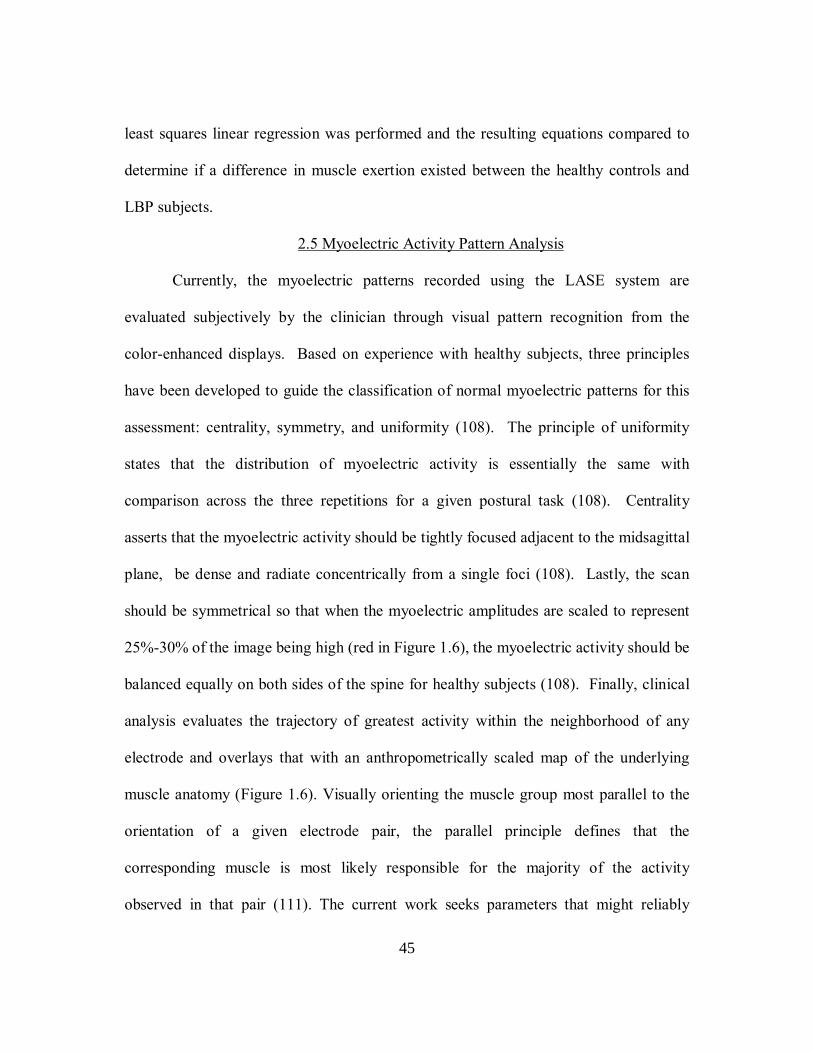
45

least squares linear regression was performed and the resulting equations compared to

determine if a difference in muscle exertion existed between the healthy controls and

LBP subjects.

2.5 Myoelectric Activity Pattern Analysis

Currently, the myoelectric patterns recorded using the LASE system are

evaluated subjectively by the clinician through visual pattern recognition from the

color-enhanced displays. Based on experience with healthy subjects, three principles

have been developed to guide the classification of normal myoelectric patterns for this

assessment: centrality, symmetry, and uniformity (108). The principle of uniformity

states that the distribution of myoelectric activity is essentially the same with

comparison across the three repetitions for a given postural task (108). Centrality

asserts that the myoelectric activity should be tightly focused adjacent to the midsagittal

plane, be dense and radiate concentrically from a single foci (108). Lastly, the scan

should be symmetrical so that when the myoelectric amplitudes are scaled to represent

25%-30% of the image being high (red in Figure 1.6), the myoelectric activity should be

balanced equally on both sides of the spine for healthy subjects (108). Finally, clinical

analysis evaluates the trajectory of greatest activity within the neighborhood of any

electrode and overlays that with an anthropometrically scaled map of the underlying

muscle anatomy (Figure 1.6). Visually orienting the muscle group most parallel to the

orientation of a given electrode pair, the parallel principle defines that the

corresponding muscle is most likely responsible for the majority of the activity

observed in that pair (111). The current work seeks parameters that might reliably

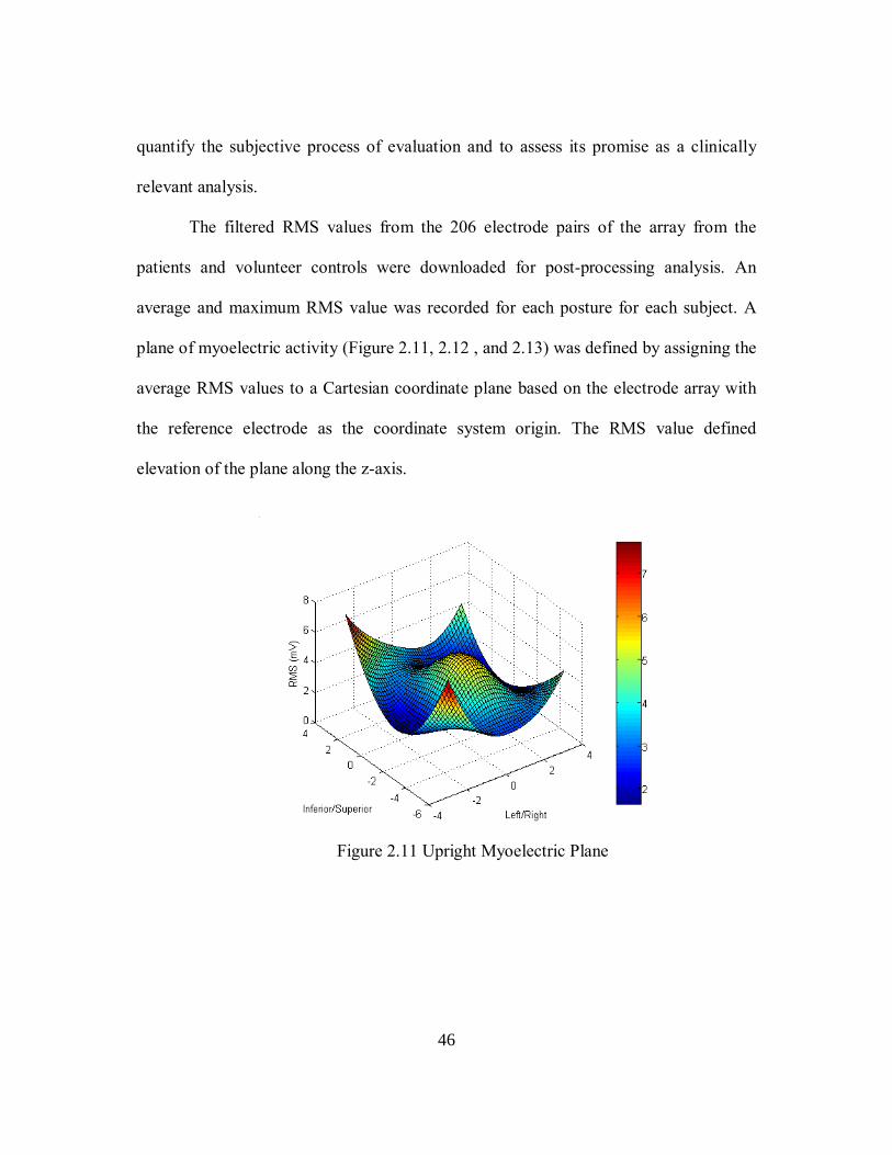
46

quantify the subjective process of evaluation and to assess its promise as a clinically

relevant analysis.

The filtered RMS values from the 206 electrode pairs of the array from the

patients and volunteer controls were downloaded for post-processing analysis. An

average and maximum RMS value was recorded for each posture for each subject. A

plane of myoelectric activity (Figure 2.11, 2.12 , and 2.13) was defined by assigning the

average RMS values to a Cartesian coordinate plane based on the electrode array with

the reference electrode as the coordinate system origin. The RMS value defined

elevation of the plane along the z-axis.

Figure 2.11 Upright Myoelectric Plane

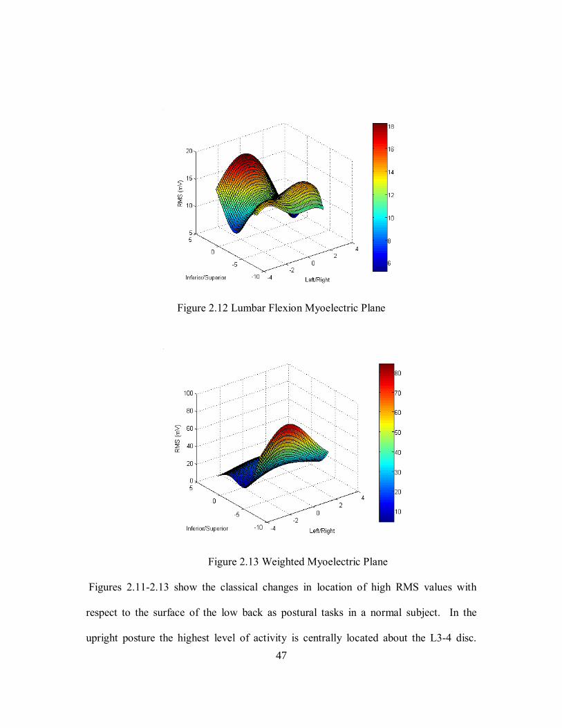
47

Figure 2.12 Lumbar Flexion Myoelectric Plane

Figure 2.13 Weighted Myoelectric Plane

Figures 2.11-2.13 show the classical changes in location of high RMS values with

respect to the surface of the low back as postural tasks in a normal subject. In the

upright posture the highest level of activity is centrally located about the L3-4 disc.

48

Then, the maximum activity shifts to the lumbar and thoracic regions of the paraspinal

muscles for the flexion and weighted tasks respectively.

To determine the myoelectric centrality and symmetry about the spine, two

parameters representing the eccentricity (i.e. directed offset, positive or negative) for the

sum of RMS values and their first moment with respect to the reference planes at L3

were defined. For purposes of this study, symmetry was defined as having an

eccentricity value of zero based on subtracting the sum of the RMS on each side of the

reference axis. The horizontal (X) axis defines vertical symmetry (ev) while the vertical

(Y) axis defines transverse symmetry (et). In addition, a weighting factor, first moment

of RMS, was created to evaluate centrality for conditions of non-zero eccentricity. That

is, greater activity on one side of the spine that is closer or farther away from the

midline (sagittal) or the horizontal (transverse) planes can be represented by a multiple

of the moment arm and the RMS value. Similarly, first moment activity that was more

or less above the axis at the coordinate center was separately determined. The first

moments were calculated by taking the scalar difference between the voltage values for

each set (defined as the matching positional vector on either side of the sagittal or

transverse planes) of electrode pairs for each posture. Together, these values in the

myoelectric plane provided a vectorial representation of the electrical activity arising

from the back during a given task. A detailed listing of the algorithm used to determine

the eccentric quantity can be found in Appendix A. In addition to the eccentric values,

the first moment of eccentricity (EM, Equations 13 and 14 ) for the muscle activity was

determined by multiplying the eccentric value by its corresponding distance from the

49

spine. For comparison, absolute value variables were determined by taking the absolute

value of each of the aforementioned variables for each subject. Table 2.4 gives the

variables and their corresponding definitions.

For the sagittal plane:

Eccentricity (ev) = evi= Σ Lvi - Rvi (13)

1st moment of ev (EMvi)= Σ (Lvi*lvi)-( Rvi*rvi) (14)

where Lvi =Voltage value for the ith pair on the left side, (i=1:3)

lyi = distance of the ith left side pair to the spine, given in cm as

defined by LASE specification manual

Rvi = Voltage value for the ith pair on the right side, (i=1:3)

rvi = distance of the ith right side pair to the spine, given in cm as

defined by LASE specification manual

For the transverse plane:

Eccentricity (et) = Σ Sti Iti (15)

1st moment of et EMti=Σ ( Sti*lti) ( Iti*rti) (16)

where Sti =Voltage value for the ith pair on the superior spine, (i=1:3)

lti = distance of the ith superior pair to the spine, given in cm as

defined by LASE specification manual

Iti = Voltage value for the ith pair on the inferior spine, (i=1:3)

rti = distance of the ith inferior pair to the spine, given in cm as

defined by LASE specification manual

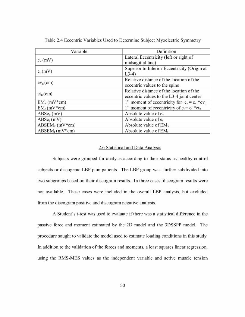
50

Table 2.4 Eccentric Variables Used to Determine Subject Myoelectric Symmetry

Variable Definition

ev (mV) Lateral Eccentricity (left or right of midsagittal line)

et (mV) Superior to Inferior Eccentricity (Origin at L3-4)

evn (cm) Relative distance of the location of the eccentric values to the spine

etn (cm) Relative distance of the location of the eccentric values to the L3-4 joint center

EMv (mV*cm) 1st moment of eccentricity for ev = ev *evn EMt (mV*cm) 1st moment of eccentricity of et = et *etn ABSev (mV) Absolute value of ev ABSet (mV) Absolute value of et ABSEMv (mV*cm) Absolute value of EMv ABSEMt (mV*cm) Absolute value of EMt

2.6 Statistical and Data Analysis

Subjects were grouped for analysis according to their status as healthy control

subjects or discogenic LBP pain patients. The LBP group was further subdivided into

two subgroups based on their discogram results. In three cases, discogram results were

not available. These cases were included in the overall LBP analysis, but excluded

from the discogram positive and discogram negative analysis.

A Students t-test was used to evaluate if there was a statistical difference in the

passive force and moment estimated by the 2D model and the 3DSSPP model. The

procedure sought to validate the model used to estimate loading conditions in this study.

In addition to the validation of the forces and moments, a least squares linear regression,

using the RMS-MES values as the independent variable and active muscle tension

51

components as the dependent variable was performed to predict the expected muscle

load in both the healthy and LBP groups.

Finally, a stepwise logistic regression (logit) model was used to estimate the

influence of various anatomical and physiological attributes on a subjects group

assignment (healthy versus LBP). This type of analysis was chosen due to the binary

nature of the subject population categorization in the study. The model was constructed

and analyzed with robust standard errors that are more conservative and account for

heteroskedasticity (123). The independent variables included were: subject height,

weight, body mass index (BMI), posture, discogram result (positive versus negative) as

well as each of the measured variables listed in Table 2.3. The logit model served to

establish which of the several parameters were significantly associated with

membership in the low back pain discography candidate group.

52

CHAPTER 3

RESULTS

The current study was undertaken to compare the myoelectric characteristics of

discogenic low back pain from those of healthy control subjects performing standard,

sagitally symmetric tasks. sEMG tests were performed on 19 men and 19 women

whose ages ranged from 23-61 years (Table 3.1and 3.2). Mean subject height and

weight were 170.28 ± 10.72 centimeters and 77.44 ± 16.67 kg respectively. There was

no significant difference in age or height between the sample groups; however, there

was a significant difference found between the healthy versus LBP groups in terms of

weight (p=0.029) with the patients being heavier. The healthy group had a mean weight

of 72.55 ± 15.09 kg and LBP group mean of 82.88 ± 17.05 kg. Table 3.1 displays the

characteristics of the subjects by group.

Table 3.1 Characteristics of LBP patients and healthy subjects (mean (SD))

Variable Healthy Subjects LBP Patients n = 20 Disco + (n = 12) Disco (n = 3)

Age (years) 40.55 (10.74) 41.08 (10.29) 40.67 (4.62) Weight (kg) 72.55 (15.09) 81.83 (18.27) 84.52 (22.11) Height (cm) 170.18 (10.55) 168.80 (12.44) 175.26 (9.16) VAS LBP 0.1 (0.15) 5.30 (2.71) 2.30 (2.40) VAS leg pain 0.05 (0.01) 4.08 (2.67) 0.60 (0.85)

53

3.1 Biomechanical Model

The mean passive loading conditions acting on the L5-S1 disc from the three

repetitions were calculated from both the 3D and 2D models for each of the three

standardized postures (upright, weighted, and flexion). The association of forces and

moments between the 3D model and the 2D static model were assessed by using

Pearson’s correlation for comparability in response and a Student’s t-test analyzed the

differences between the outputs of the two models (Table 3.1). Acceptable correlation

was found for both the passive disc compression (R2 = 0.831) and moment generation

(R2 = 0.743). No systematic bias existed for the compression forces (p=0.374), however

a significant difference was found for the moments (p=4.43 x 10-5) respectively.

Although there was no significant difference between means for the compressive forces

or the moments, the 2D model did slightly underestimate the compressive force of the

disc by 0.40% when compared to the 3D model. Further, the moments were

overestimated by 7.05% in contrast to the 3D model.

Table 3.2 Comparison of Mean Forces and Moments for the 3D and 2D Biomechanical Models

3DSS Model 2D Model Mean SD Mean SD T statistic P-value Force (N) 287.34 67.90 286.19 62.50 -0.321 0.748 Moment (Nm) 52.69 10.60 56.68 12.40 4.144 4.43 x 10-5

Active forces generated by estimated muscular tension was extracted from the

3D biomechanical model and served as input to a regression model along with the

RMS values measured by the LASE sEMG system. A regression was performed using

both the average RMS across the 206 electrode and the maximum RMS value for each

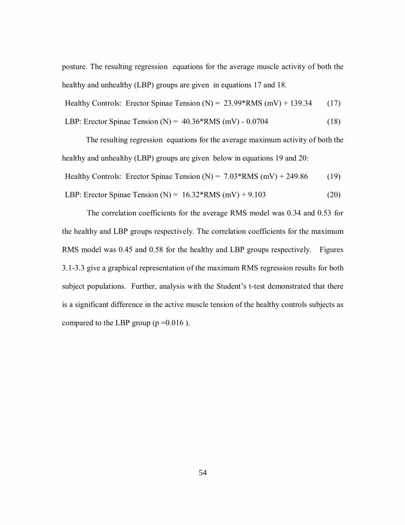
54

posture. The resulting regression equations for the average muscle activity of both the

healthy and unhealthy (LBP) groups are given in equations 17 and 18.

Healthy Controls: Erector Spinae Tension (N) = 23.99*RMS (mV) + 139.34 (17)

LBP: Erector Spinae Tension (N) = 40.36*RMS (mV) - 0.0704 (18)

The resulting regression equations for the average maximum activity of both the

healthy and unhealthy (LBP) groups are given below in equations 19 and 20:

Healthy Controls: Erector Spinae Tension (N) = 7.03*RMS (mV) + 249.86 (19)

LBP: Erector Spinae Tension (N) = 16.32*RMS (mV) + 9.103 (20)

The correlation coefficients for the average RMS model was 0.34 and 0.53 for

the healthy and LBP groups respectively. The correlation coefficients for the maximum

RMS model was 0.45 and 0.58 for the healthy and LBP groups respectively. Figures

3.1-3.3 give a graphical representation of the maximum RMS regression results for both

subject populations. Further, analysis with the Students t-test demonstrated that there

is a significant difference in the active muscle tension of the healthy controls subjects as

compared to the LBP group (p =0.016 ).

55

0

200

400

600

800

1000

1200

1400

1600

1800

0 50 100 150 200

RMS (mV)

Hea

lthy

Erec

tor

Spi

nae

Mus

cle

Tens

ion

(N) Healthy Erector Spinae

Muscle Tension (N)Predicted Healthy ErectorSpinae Muscle Tension (N)

0

200

400

600

800

1000

1200

1400

1600

0 20 40 60 80 100

RMS (mV)

LBP

Ere

ctor

Spi

nae

Mus

cle

Tens

ion

(N)

LBP Erector SpinaeMuscle Tension (N)Predicted LBP ErectorSpinae Muscle Tension (N)

Figure 3.1 Raw and Linear regression data of healthy subject maximum muscle activity versus active muscle tension

Figure 3.2 Raw and Linear regression data of LBP subject maximum muscle activity versus active muscle tension

56

Figure 3.3 Comparison of the linear regression of the maximum muscle activity versus

active muscle tension for healthy and LBP subjects

Both subject populations were divided by gender such that active muscle

tension and resulting moment generation could be evaluated by subject sex. Table 3.3

summarizes the results of the gender differences. No difference was found between the

healthy versus LBP subjects for the men (p = 0.014) or women (p =0.035 ) respectively.

Also, no difference existed between the male versus female population for forces (p =

.24), however systemic bias did exist for the moments (p = 3.61x10-5).

Table 3.3 Comparison of male and female active muscle tension and moment values

Sex Healthy LBP

Force (N) Women Men

585.54 (234.36) 582.66 (266.69)

616.13(357.34) 671.35 (336.17)

Moment (Nm) Women Men

2185.32 (933.61) 2197.30(973.49)

2318.37 (1390.08) 2512.52 (1218.44)

3.2 Myoelectric Eccentricity Analysis

The mean level of muscle activity (RMS) for each postural task was calculated

for each group (healthy, LBP, positive discogram and negative discogram). Table 3.4

57

0.00

10.00

20.00

30.00

40.00

50.00

60.00

70.00

80.00

90.00

Upright Flexion Weighted

Posture

Mea

n RM

S (m

V)

HealthyLBPDisco +Disco -

provides central tendency and dispersion of each group. Figure 3.4 graphs the change in

maximum muscle activity with respect to posture.

Table 3.4 Maximum RMS activity for each subject group (Mean (SD)) Posture RMS (mV)

Healthy LBP Disco + Disco - Upright 17.53 (6.68) 17.22 (7.27) 16.97(8.62) 18.33(4.84) Flexion 45.27(15.84) 40.43(13.31) 41.33(15.20) 40.44(13.80)

Weighted 79.82(39.33) 58.98(15.27) 56.33(16.89) 69.89(11.67)

Figure 3.4 Graphical representation of posture versus mean maximum RMS

To evaluate any differences between RMS activity of men and women, each

subject population was divided by gender and compared (i.e. healthy men versus LBP

men and healthy women versus LBP women). There was statistical significance found

between groups, healthy versus LBP p= 0.20 and 0.08 for the men and women

respectively. Also, no difference in RMS activity across postural tasks existed between

male versus female populations (p = 0.36).

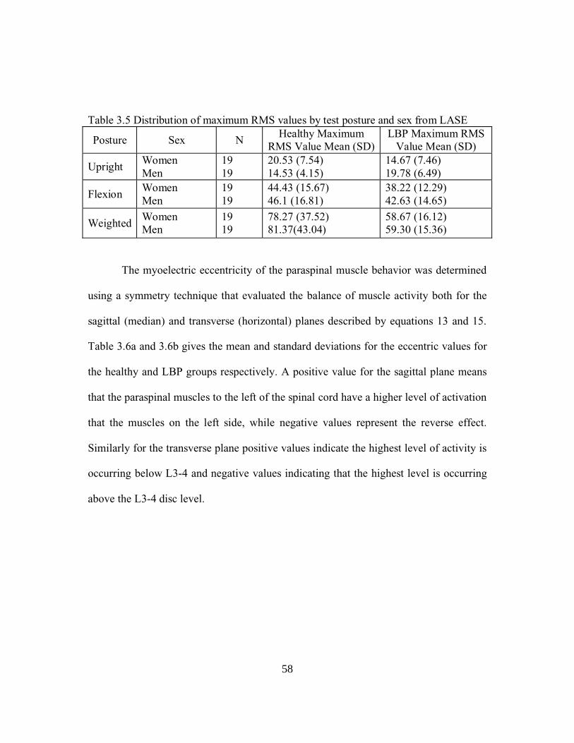
58

Table 3.5 Distribution of maximum RMS values by test posture and sex from LASE

Posture Sex N Healthy Maximum RMS Value Mean (SD)

LBP Maximum RMS Value Mean (SD)

Upright Women Men

19 19

20.53 (7.54) 14.53 (4.15)

14.67 (7.46) 19.78 (6.49)

Flexion Women Men

19 19

44.43 (15.67) 46.1 (16.81)

38.22 (12.29) 42.63 (14.65)

Weighted Women Men

19 19

78.27 (37.52) 81.37(43.04)

58.67 (16.12) 59.30 (15.36)

The myoelectric eccentricity of the paraspinal muscle behavior was determined

using a symmetry technique that evaluated the balance of muscle activity both for the

sagittal (median) and transverse (horizontal) planes described by equations 13 and 15.

Table 3.6a and 3.6b gives the mean and standard deviations for the eccentric values for

the healthy and LBP groups respectively. A positive value for the sagittal plane means

that the paraspinal muscles to the left of the spinal cord have a higher level of activation

that the muscles on the left side, while negative values represent the reverse effect.

Similarly for the transverse plane positive values indicate the highest level of activity is

occurring below L3-4 and negative values indicating that the highest level is occurring

above the L3-4 disc level.

59

Table 3.6a Eccentric values for the healthy group

Table 3.6b Eccentric values for the LBP group

Upright

et (mV)

ev (mV)

EMT (mV*cm)

EMV (mV*cm)

ABS et (mV)

ABS ev (mV)

ABS EMT

(mV*cm)

ABS EMV

(mV*cm) Mean 12.43 45.23 43.54 191.79 19.30 53.60 92.46 248.67 SD 24.67 57.91 122.60 279.35 19.36 49.83 89.60 227.31

Flexion

et (mV)

ev (mV)

EMT (mV*cm)

EMV (mV*cm)

ABS et (mV)

ABS ev (mV)

ABS EMT

(mV*cm)

ABS EMV

(mV*cm) Mean 31.38 -50.0 173.31 -308.46 48.48 115.80 223.94 611 SD 48.92 153.2 206.47 750.97 30.92 109.6 146.49 520.73

Weighted

et (mV) ev (mV)

EMT (mV*cm)

EMV (mV*cm)

ABS et (mV)

ABS ev (mV)

ABS EMT

(mV*cm)

ABS EMV

(mV*cm) Mean 66.17 204.3 272 1044.27 72.43 222.8 433.25 1123.69 SD 88.89 185.6 731.27 951.91 83.58 161.7 644.24 851.41

Upright

et (mV) ev (mV) EMT

(mV*cm)EMV

(mV*cm)ABS et (mV)

ABS ev (mV)

ABS EMT (mV*cm)

ABS EMV

(mV*cm) Mean 8.78 28.407 55.46 89.58 17.81 49.82 78.24 232.78 SD 19.82 59.738 78.77 285.03 11.76 42.38 54.58 179.9

Flexion

et (mV) ev (mV) EMT

(mV*cm)EMV

(mV*cm)ABS et (mV)

ABS ev (mV)

ABS EMT (mV*cm)

ABS EMV

(mV*cm) Mean 14.13 26.611 149 64.51 55.17 82.76 291.64 426.55 SD 74.523 136.07 317.98 642.36 50.42 109.61 185.9 473.69

Weighted

et (mV) ev (mV) EMT

(mV*cm)EMV

(mV*cm)ABS et (mV)

ABS ev (mV)

ABS EMT (mV*cm)

ABS EMV

(mV*cm) Mean 53.13 214.59 315.81 1007.69 88.65 218.44 391.04 1034.26 SD 101.77 158 340.93 746.41 70.88 152.31 244.81 706.88

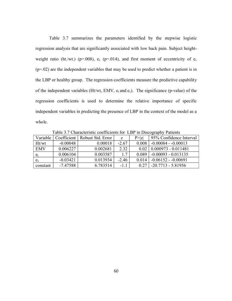
60

Table 3.7 summarizes the parameters identified by the stepwise logistic

regression analysis that are significantly associated with low back pain. Subject height-

weight ratio (ht./wt.) (p=.008), ev (p=.014), and first moment of eccentricity of ev

(p=.02) are the independent variables that may be used to predict whether a patient is in

the LBP or healthy group. The regression coefficients measure the predictive capability

of the independent variables (Ht/wt, EMV, et and ev). The significance (p-value) of the

regression coefficients is used to determine the relative importance of specific

independent variables in predicting the presence of LBP in the context of the model as a

whole.

Table 3.7 Characteristic coefficients for LBP in Discography Patients Variable Coefficient Robust Std. Error z P>|z| 95% Confidence IntervalHt/wt -0.00048 0.00018 -2.67 0.008 -0.00084 - -0.00013 EMV 0.006227 0.002681 2.32 0.02 0.000973 - 0.011481 et 0.006104 0.003587 1.7 0.089 -0.00093 - 0.013135 ev -0.03421 0.013934 -2.46 0.014 -0.06152 - -0.00691 constant -7.47588 6.783514 -1.1 0.27 -20.7713 - 5.81956

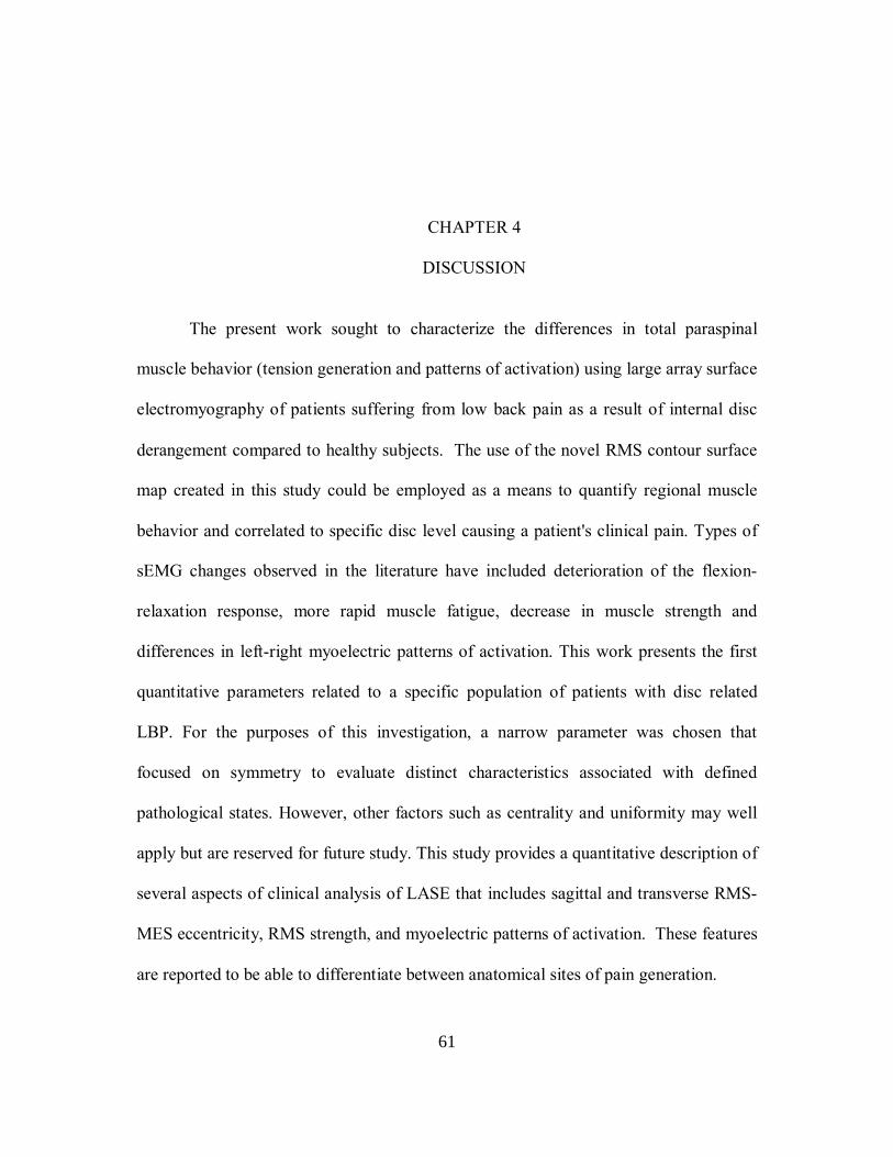
61

CHAPTER 4

DISCUSSION

The present work sought to characterize the differences in total paraspinal

muscle behavior (tension generation and patterns of activation) using large array surface

electromyography of patients suffering from low back pain as a result of internal disc

derangement compared to healthy subjects. The use of the novel RMS contour surface

map created in this study could be employed as a means to quantify regional muscle

behavior and correlated to specific disc level causing a patient's clinical pain. Types of

sEMG changes observed in the literature have included deterioration of the flexion-

relaxation response, more rapid muscle fatigue, decrease in muscle strength and

differences in left-right myoelectric patterns of activation. This work presents the first

quantitative parameters related to a specific population of patients with disc related

LBP. For the purposes of this investigation, a narrow parameter was chosen that

focused on symmetry to evaluate distinct characteristics associated with defined

pathological states. However, other factors such as centrality and uniformity may well

apply but are reserved for future study. This study provides a quantitative description of

several aspects of clinical analysis of LASE that includes sagittal and transverse RMS-

MES eccentricity, RMS strength, and myoelectric patterns of activation. These features

are reported to be able to differentiate between anatomical sites of pain generation.

62

The spinal stabilizing system can be divided into three main components: 1) the

spinal column, which provides intrinsic stability, 2) spinal muscles, providing dynamic

stability and 3) neural control unit, assessing requirements for stability, initiating

motion and coordinating muscle response (124). Under normal conditions these systems

coordinate and provide the needed mechanical stability; however, if one system fails,

the others must compensate for that loss (124). An example of a failed system per

above, is that of internal disc derangement, where the spinal column may loose stability

causing the spinal muscles to exhibit a change in myoelectric activity and increase

spinal stiffness to prevent failure of the system. Figure 4.1 is a X-ray showing how the

disc tear caused by internal disc derangement makes the spine unstable by allowing for

excessive motion in extension. In patients where pathology exists but the spine remains

stable, the muscles may react with increased myoelectric activity in response to painful

stimuli (125). Thus, muscle action in these patients may also provide a mechanism for

stiffening and protecting the spine from additional injury.

Figure 4.1 X-ray of an unstable deranged disc in extension (black area in the disc is the tear)

63

The three standardized test postures provided monotonically increasing loading

of the spine for each subject. As a result, the passive loads acting on the spine at L5/S1

were proportional to subject stature and posture. Differences in muscle reaction between

groups represent activation caused by other factors, in this case, probably pain.

Normalization was not used for the MES activity attained from the LASE studies

because no direct comparison between individual subjects were made. The postural

tasks that were chose rely on the involuntary contraction of the paraspinal muscles to

maintain trunk stability. In contrast, normalization is typically measured as a given

percentage of a subjects maximum voluntary contraction (MVC) and this protocol did

not approach MVC. EMG normalization also requires a moderate amount of subject

training to assure the accuracy of the MVC measure, else erroneous data may result.

The biomechanical models partitioned activity into a first approximation of load from

muscle versus posture/stature. When the subjects were grouped as to the presence or

absence of LBP, a statistical regression of the mean and maximum muscle activity

(RMS) versus active muscle load from the LBP and healthy control group was

conducted. The regression yielded different predictive equations for active muscle

loads for each subject population. The mean RMS yielded a better estimation of the

data (R2 = 0.45 ), however, there was a negative intercept for the LBP subjects, which is

misleading as to the physiological significance for the zero muscle activity condition.

In the maximum RMS regression, both models (Figure 3.3) had non zero intercepts

suggesting that there is tension in the muscle in the non-contracted state. The nonzero

intercept may be correlated with the passive loads of the muscle tendon group, however,

64

future study would be needed to confirm this assumption. In Figures 3.1 and 3.2 there

are clusters of data resulting from the significant change in postural tasks which causes

both the offset of the y-intercept and more curvilinear graph. This observation appears

to indicate that a linear regression model may not be sufficient for the data collected in

this study, and a more curvilinear model should be explored in future work. Further,

individual regressions for each subject accounting for posture may correct the offset,

however, would not yield the necessary predictive equations for the subjects groups as a

whole as was sought in this investigation. Overall, the findings related to the

biomechanical models are in agreement with the literature, which shows that patients

with LBP present an increase in active muscle load as compared to healthy subjects.

The equations provide an estimate of the relative increased spine load derived from

myoelectric behavior beyond biomechanical demands of the test tasks. Such

information may be useful in future study to understand the factors associated with

compensation for instability or pain.

The results of the sEMG screening revealed that the symmetry/eccentricity of

the RMS-MES distribution and the first moment of eccentricity about the sagittal plane

coupled with subject stature (height-weight ratio) are correlated with the presence or

absence of LBP. The present patient group is a sample representing a common group of

people with chronic disc-related LBP. The mean level of muscle activity in the LBP

group was 10.33% and 19.41% lower than the healthy group for the lumbar flexion and

weighted postures respectively. Separating the patients with negative discogram result

from the LBP group, the level of muscle activity was 23.9% lower than the activity of

65

the pain free group. This increased level of significance suggests that the intensity of

muscle load is correlated with a positive discogram result. Because the sample was

dominated by positive discograms, this observation should be tested in future work.

Future analysis of these myoelectric data may identify other parameters related to

location or intensity of muscle action within the stabilizing system of the lumbar region

that further differentiates the groups. The sample size for this study was relatively

small, yielding disproportion between positive and negative discogram results.

Moreover, the sample of subjects recruited was biased by the fact that they were being

sent for discography on the basis of clinical suspicion expecting a positive report. As a

result, while there appeared to be differences in the mean of RMS values, they did not

reach statistical significance. Accumulation of additional negative discogram subjects

will permit the determination of any utility for myoelectric parameters in discrimination

of positive from negative patients. Table 3.5 shows that grouping the subjects by

gender does not yield a systemic bias between the healthy and LBP groups.

Additionally, no systemic bias was found between the RMS activity of the total male

(including healthy and LBP men) and the total female (including healthy and LBP)

populations. The absence of differences based on age and gender probably reflects the

recruitment of subjects resulting in comparable distributions between groups. This

observation implies that age and gender are not important factors in myoelectric

behaviors despite the fact that incidence and prevalence of care seeking do show

statistically different trends (129).

66

The statistically different parameters (ev, height-weight ratio, and EM V)

suggest that they may serve as predictors to separate patients from healthy people. The

strongest parameter among the EMG variables was the symmetry about the sagittal

plane. Based on the results, the LBP group demonstrated a significant increase in the

left-right RMS-MES difference of the muscles. The present analysis supports previous

findings (3-5) in that both the myoelectric balance of LBP patients and height-weight

ratio differ from that of healthy control subjects. Studies (130, 131) have shown that

there is a prevalence of obesity in LBP patient populations. Successful stratification of a

new sample of healthy and discogenic pain subjects using these parameters will be

necessary to confirm the results for clinical use in diagnosis. Ideally, the eccentricity

for a sagitally symmetric task for healthy subjects would be zero, however, as can be

seen from Table 3.4a, the subjects in the present study deviated from this expectation.

This finding suggests that the ideal left-right symmetry for healthy subjects is not

supported. Other factors that may influence the symmetry of MES activation of the

paraspinal muscles include but are not limited to: left/right handedness, spinal

curvature, and past physical activity (i.e. whether the subject was a participant in sports

that required repetitive asymmetric tasks). Future study of these factors may lead to the

determination of the level of influence each has on eccentricity.

Although the present study was successful in identifying the difference in the

overall behavior of the muscles between LBP patients and healthy control subjects, it

failed to discriminate between subjects with positive and negative discogram result. It

could be postulated that no difference exists; however, given the small sample size of

67

negative discogram results (20% of LBP subjects); this conclusion seems to be

premature. Increasing the sample size of the LBP group would give a better perspective

for characterizing if any difference exists. The patient population was limited to those

subjects with the specific diagnosis of internal disc derangement. Once there is a

clearly defined method associating the patterns of activation with the result of the

discogram, the study can be expanded to include other pathologies such as herniation or

sacroiliac joint syndrome; allowing for the determination as to whether sEMG has

specificity of diagnosis.

68

CHAPTER 5

CONCLUSIONS

As shown in Figure 3.3, an increase in muscle activity causes a more

disproportionate increase in active muscle loads of LBP patients versus healthy control

subjects. Furthermore, parameters derived from contour maps of the lumbar regional

muscle behavior appear to quantitatively describe useful patterns that may differentiate

LBP patients versus healthy subjects. The main result of this work is the discovery that

the overall decrease in myoelectric symmetry may be a distinguishing characteristic of

LBP patients. The data attained from the LASE sEMG strongly supports that body mass

and a reduction in the sagittal eccentricity are different between the LBP and healthy

control subjects. The absence of statistical difference between the male and female

population suggests that gender is not linked to the myoelectric behavior of patients

seeking treatment for disc-related back pain. The greatest weakness of this study is the

small sample population of LBP patients and the need to perform confirmation of the

step-wise regression model with a subsequent sample. The importance of this work

relies on the fact that its results suggest that there are different types of information

gained from regional mapping of the muscle behavior than there is from small segment

sampling at isolated spine levels. It is at least conceivable that there exists patients who

have different patterns of activation than subjects tested in this study.

69

It may also be fruitful for future work to examine other quantitative

characteristics of RMS surface maps to differentiate the behavior of muscle activity. In

contrast to small area surface electromyography, LASE may provide additional

information helpful in classifying type and severity of low back injury leading to the

development of more successful treatment methods. Combined with the work of

Finneran et al, which showed clear distinctions for patients with lumbar facet disorders,

the quantitative parameters found in this study establishes a foundation for the use of

LASE as a viable diagnostic technique for evaluating LBP patients.

70

APPENDIX A

MATLAB PROGRAMS

71

% This file will calculate the forces and moments at the L5/S1, L4/5 and % L3/4 disc levels for each posture upright, flexion and weighted %Input of subject data D=[Ht (m) Wt (kg)] X=xlsread('K:\Thesis\Matlab analysis\Data\Height_Weight');%where col 1=subject no. col 2=height, col 3 =weight, col 4=AP measurement, col 5=arm length, col 6=hand length X(:,1)=[]; %deletes subject numbers and shifts all columns to the left %X(1,:)=[]; %deletes 1st row of x in case it coMES through as a NaN value %(row 1 contains the headings [n,m]=size(X); %Angles a5=37*(pi/180); a5f=42*(pi/180); %L5-S1 a4=40*(pi/180); a4f=42.5*(pi/180); %L4-5 a3=0*(pi/180); a3f=2.5*(pi/180); %L3-4 %metric units for i=1:n %Force Calculations g=9.81; %gravity FUB(i,:)=[((X(i,2)*g)*.468) ((X(i,2)*g)*.439) ((X(i,2)*g)*.413)]; % Weight of the head, neck and trunk at each disc level [L5/S1 L4/5 L3-4] %Calculation of the total forces at the disc levels for each posture FU(i,:)=[(FUB(i,1))*cos(a5) (FUB(i,2))*cos(a4) (FUB(i,3))*cos(a3)]; %Upright FF(i,:)=[(FUB(i,1))*cos(a5f) (FUB(i,2))*cos(a4f) (FUB(i,3))*cos(a3f)]; %Flexion HL=44.48; %hand load in Newtons FW(i,:)=[((FUB(i,1))+HL)*cos(a5) ((FUB(i,2))+HL)*cos(a4) ((FUB(i,3))+HL)*cos(a3)]; %Weighted %Moment Calculations %Flexion Input forces FH(i,:)=[(X(i,2)*.062)*cos(a5f) (X(i,2)*.062)*cos(a4f) (X(i,2)*.062)*cos(a3f)]*g; %head FA(i,:)=[(X(i,2)*.051)*cos(a5f) (X(i,2)*.051)*cos(a4f) (X(i,2)*.051)*cos(a3f)]*g; %arm FT(i,:)=[(X(i,2)*.355)*cos(a5f) (X(i,2)*.326)*cos(a4f) (X(i,2)*.3)*cos(a3f)]*g; %trunk th=[a5f a4f a3f]; %angle at each disc level in radians rh(i,:)=[tan(th(1,1))*(0.406*X(i,1)) tan(th(1,2))*((0.406*X(i,1)-.366)) tan(th(1,3))*((0.406*X(i,1)-.729))]*.01; %moment arm from L5-S1, L4-5, L3-4 COM to head COM raf(i,:)=[tan(th(1,1))*(0.288*X(i,1)) tan(th(1,2))*((0.288*X(i,1)-.366)) tan(th(1,3))*((0.288*X(i,1)-.729))]*.01;%%moment arm from L5-S1, L4-5, L3-4 COM to arm COM rt(i,:)=[tan(th(1,1))*(0.604*X(i,1)) tan(th(1,2))*((0.604*X(i,1)-.366)) tan(th(1,3))*((0.604*X(i,1)-.729))]*.01; %moment arm from L5-S1 COM to trunk COM %Calcualte moments at each level MF(i,:)=[(FH(i,1)*rh(i,1))+(FA(i,1)*raf(i,1))+(FT(i,1)*rt(i,1)) (FH(i,2)*rh(i,2))+(FA(i,2)*raf(i,2))+(FT(i,2)*rt(i,2)) (FH(i,3)*rh(i,3))+(FA(i,3)*raf(i,3))+(FT(i,3)*rt(i,3))]; %Weighted raw(i,:)=[((X(i,4)+X(i,5))*.413)+(0.5*X(i,3))]; rw(i,:)=[X(i,4)+(0.494*(X(i,5)))+(0.5*(X(i,3)))]; W(i,:)=[HL*cos(a5) HL*cos(a4) HL*cos(a3)];

72

MW(i,:)=[(FA(i,1)*raw(i,:))+(W(i,1)*rw(i,:)) (FA(i,2)*raw(i,:))+(W(i,2)*rw(i,:)) (FA(i,3)*raw(i,:))+(W(i,3)*rw(i,:))]; end %Regression Analysis R1=XLSREAD('C:\Documents and Settings\Compaq_Owner\Desktop\Thesis\Matlab analysis\Data\sub1'); R2=XLSREAD('C:\Documents and Settings\Compaq_Owner\Desktop\Thesis\Matlab analysis\Data\sub2'); R3=XLSREAD('C:\Documents and Settings\Compaq_Owner\Desktop\Thesis\Matlab analysis\Data\sub3'); R4=XLSREAD('C:\Documents and Settings\Compaq_Owner\Desktop\Thesis\Matlab analysis\Data\sub4'); R5=XLSREAD('C:\Documents and Settings\Compaq_Owner\Desktop\Thesis\Matlab analysis\Data\sub6'); R6=XLSREAD('C:\Documents and Settings\Compaq_Owner\Desktop\Thesis\Matlab analysis\Data\sub10'); R7=XLSREAD('C:\Documents and Settings\Compaq_Owner\Desktop\Thesis\Matlab analysis\Data\sub11'); R8=XLSREAD('C:\Documents and Settings\Compaq_Owner\Desktop\Thesis\Matlab analysis\Data\sub12'); R9=XLSREAD('C:\Documents and Settings\Compaq_Owner\Desktop\Thesis\Matlab analysis\Data\sub13'); R10=XLSREAD('C:\Documents and Settings\Compaq_Owner\Desktop\Thesis\Matlab analysis\Data\sub15'); R11=XLSREAD('C:\Documents and Settings\Compaq_Owner\Desktop\Thesis\Matlab analysis\Data\sub21'); R12=XLSREAD('C:\Documents and Settings\Compaq_Owner\Desktop\Thesis\Matlab analysis\Data\sub23'); R13=XLSREAD('C:\Documents and Settings\Compaq_Owner\Desktop\Thesis\Matlab analysis\Data\sub24'); R14=XLSREAD('C:\Documents and Settings\Compaq_Owner\Desktop\Thesis\Matlab analysis\Data\sub25'); R15=XLSREAD('C:\Documents and Settings\Compaq_Owner\Desktop\Thesis\Matlab analysis\Data\sub29'); R16=XLSREAD('C:\Documents and Settings\Compaq_Owner\Desktop\Thesis\Matlab analysis\Data\sub32'); R17=XLSREAD('C:\Documents and Settings\Compaq_Owner\Desktop\Thesis\Matlab analysis\Data\sub33'); R18=XLSREAD('C:\Documents and Settings\Compaq_Owner\Desktop\Thesis\Matlab analysis\Data\sub34'); R19=XLSREAD('C:\Documents and Settings\Compaq_Owner\Desktop\Thesis\Matlab analysis\Data\sub14'); R20=XLSREAD('C:\Documents and Settings\Compaq_Owner\Desktop\Thesis\Matlab analysis\Data\sub28'); R21=xlsread('C:\Documents and Settings\Compaq_Owner\Desktop\Thesis\Matlab analysis\Data\sub5'); R22=xlsread('C:\Documents and Settings\Compaq_Owner\Desktop\Thesis\Matlab analysis\Data\sub7'); R23=xlsread('C:\Documents and Settings\Compaq_Owner\Desktop\Thesis\Matlab analysis\Data\sub16'); R24=xlsread('C:\Documents and Settings\Compaq_Owner\Desktop\Thesis\Matlab analysis\Data\sub17'); R25=xlsread('C:\Documents and Settings\Compaq_Owner\Desktop\Thesis\Matlab analysis\Data\sub18'); R26=xlsread('C:\Documents and Settings\Compaq_Owner\Desktop\Thesis\Matlab analysis\Data\sub19'); R27=xlsread('C:\Documents and Settings\Compaq_Owner\Desktop\Thesis\Matlab analysis\Data\sub22');

73

R28=xlsread('C:\Documents and Settings\Compaq_Owner\Desktop\Thesis\Matlab analysis\Data\sub26'); R29=xlsread('C:\Documents and Settings\Compaq_Owner\Desktop\Thesis\Matlab analysis\Data\sub30'); R30=xlsread('C:\Documents and Settings\Compaq_Owner\Desktop\Thesis\Matlab analysis\Data\sub31'); R31=xlsread('C:\Documents and Settings\Compaq_Owner\Desktop\Thesis\Matlab analysis\Data\sub35'); R32=xlsread('C:\Documents and Settings\Compaq_Owner\Desktop\Thesis\Matlab analysis\Data\sub36'); R33=xlsread('C:\Documents and Settings\Compaq_Owner\Desktop\Thesis\Matlab analysis\Data\sub37'); R34=xlsread('C:\Documents and Settings\Compaq_Owner\Desktop\Thesis\Matlab analysis\Data\sub38'); R35=xlsread('C:\Documents and Settings\Compaq_Owner\Desktop\Thesis\Matlab analysis\Data\sub39'); R36=xlsread('C:\Documents and Settings\Compaq_Owner\Desktop\Thesis\Matlab analysis\Data\sub41'); R37=xlsread('C:\Documents and Settings\Compaq_Owner\Desktop\Thesis\Matlab analysis\Data\sub42'); R38=xlsread('C:\Documents and Settings\Compaq_Owner\Desktop\Thesis\Matlab analysis\Data\sub43'); RMSC(:,:)=[sum(R1(:,10)) sum(R1(:,14)) sum(R1(:,18)); sum(R2(:,10)) sum(R2(:,14)) sum(R2(:,18)); sum(R3(:,10)) sum(R3(:,14)) sum(R3(:,18)); sum(R4(:,10)) sum(R4(:,14)) sum(R4(:,18)); sum(R5(:,10)) sum(R5(:,14)) sum(R5(:,18)); sum(R6(:,10)) sum(R6(:,14)) sum(R6(:,18)); sum(R7(:,10)) sum(R7(:,14)) sum(R7(:,18)); sum(R8(:,10)) sum(R8(:,14)) sum(R8(:,18)); sum(R9(:,10)) sum(R9(:,14)) sum(R9(:,18)); sum(R10(:,10)) sum(R10(:,14)) sum(R10(:,18)); sum(R11(:,10)) sum(R11(:,14)) sum(R11(:,18)); sum(R12(:,10)) sum(R12(:,14)) sum(R12(:,18)); sum(R13(:,10)) sum(R13(:,14)) sum(R13(:,18)); sum(R14(:,10)) sum(R14(:,14)) sum(R14(:,18)); sum(R15(:,10)) sum(R15(:,14)) sum(R15(:,18)); sum(R16(:,10)) sum(R16(:,14)) sum(R16(:,18)); sum(R17(:,10)) sum(R17(:,14)) sum(R17(:,18)); sum(R18(:,10)) sum(R18(:,14)) sum(R18(:,18)); sum(R19(:,10)) sum(R19(:,14)) sum(R19(:,18)); sum(R20(:,10)) sum(R20(:,14)) sum(R20(:,18))]; AF=xlsread('K:\Thesis\Matlab analysis\Data\Regression'); AF(:,1)=[]; %Regression for the pain free controls for j=1:20 FC(j,:)=AF(j,:); end RRC=[RMSC(:,1);RMSC(:,2);RMSC(:,3)]; FnewC=[FC(:,1);FC(:,2);FC(:,3)]; for n1 = 1:60 x1(n1,1) = 1; x1(n1,2) = RRC(n1); y1(n1,1) = FnewC(n1); end

74

% Use the matrix division operation. NotK: The notation x = b/A will not work. a = x1\FnewC; % Calculate the values of the final weight predicted by the equation. % Then calculate the difference between the experimental and predicted values FpredC = x1*a; res = FnewC - FpredC; % Create output fprintf('\n\n\n The coefficients a1 and a2 respectively for the Pain Free Group are: \n' ) fprintf(' a1 = %5.2e \n', a(1)) fprintf(' a2 = %5.2e \n ', a(2)) % fprintf(' Experimental Force Pain Free Predicted Force Pain Free Difference \n') % for n1 = 1:54 % fprintf(' %5.2e %5.2e %5.2e \n', FnewC(n1), FpredC(n1), res(n1)); % end % %Regression for the LBP Group RMSP(:,:)=[sum(R21(:,10)) sum(R21(:,14)) sum(R21(:,18)); sum(R22(:,10)) sum(R22(:,14)) sum(R22(:,18)); sum(R23(:,10)) sum(R23(:,14)) sum(R23(:,18)); sum(R24(:,10)) sum(R24(:,14)) sum(R24(:,18)); sum(R25(:,10)) sum(R25(:,14)) sum(R25(:,18)); sum(R26(:,10)) sum(R26(:,14)) sum(R26(:,18)); sum(R27(:,10)) sum(R27(:,14)) sum(R27(:,18)); sum(R28(:,10)) sum(R28(:,14)) sum(R28(:,18)); sum(R29(:,10)) sum(R29(:,14)) sum(R29(:,18)); sum(R30(:,10)) sum(R30(:,14)) sum(R30(:,18)); sum(R31(:,10)) sum(R31(:,14)) sum(R31(:,18)); sum(R32(:,10)) sum(R32(:,14)) sum(R32(:,18)); sum(R33(:,10)) sum(R33(:,14)) sum(R33(:,18)); sum(R34(:,10)) sum(R34(:,14)) sum(R34(:,18)); sum(R35(:,10)) sum(R35(:,14)) sum(R35(:,18)); sum(R36(:,10)) sum(R36(:,14)) sum(R36(:,18)); sum(R37(:,10)) sum(R37(:,14)) sum(R37(:,18)); sum(R38(:,10)) sum(R38(:,14)) sum(R38(:,18))]; for k=1:18 for d=20:38 FP(k,:)=AF(k,:); end end RRP=[RMSP(:,1);RMSP(:,2);RMSP(:,3)]; FnewP=[FP(:,1);FP(:,2);FP(:,3)]; for n2 = 1:54 x2(n2,1) = 1;

75

x2(n2,2) = RRP(n2); y2(n2,1) = FnewP(n2); end % Use the matrix division operation. Note: The notation x = b/A will not work. b = x2\FnewP; % Calculate the values of the final weight predicted by the equation. % Then calculate the difference between the experimental and predicted values FpredP = x2*b; resP = FnewP - FpredP; % Create output fprintf('\n\n\n The coefficients b1 and b2 respectively for the Low Back Pain Group are: \n' ) fprintf(' b1 = %5.2e \n', b(1)) fprintf(' b2 = %5.2e \n', b(2)) %fprintf(' Experimental Force LBP Predicted Force LBP Difference \n') % for n = 1:57 % fprintf(' %5.2e %5.2e %5.2e \n', FnewP(n2), FpredP(n2), resP(n2)); % end figure (1) hidden off subplot(3,1,1);plotmatrix(RRC,FnewC,'gx') title('RMS vs. Muscle Load @L5-S1 for Pain Free Controls') xlabel('RMS (mV)') ylabel('Muscle Force (N)') hold on plot(RRC,FpredC,'b.-') legend('Raw Data','Linear Regression Data',2) hold off subplot(3,1,2);plotmatrix(RRP,FnewP,'bx') title('RMS vs. Muscle Load @L5-S1 for Low Back Pain Group') xlabel('RMS (mV)') ylabel('Muscle Force (N)') hold on plot(RRP,FpredP,'g.-') legend('Raw Data','Linear Regression Data',2) hold off subplot(3,1,3);plot(RRC,FpredC,'bo-') hold on plot(RRP,FpredP,'gx-') title('Comparison of Linear Regression for Pain Free & Low Back Pain Subjects') xlabel('RMS (mV)') ylabel('Muscle Force (N)') legend('Pain Free Controls','LBP Subjects',2) hold off

76

%Contour Maps %Translation calculation rap=[-3;-6;0]; rbp=[1;1;0]; rab=[4;7;0]; Rab=[1 0 0;0 1 0;0 0 1]; R=-Rab'; Rr=R*rab; Tab=[1 0 0 0;Rr Rab]; rck=Tab*[1;rbp]; %Load data A1=XLSREAD('C:\Documents and Settings\Compaq_Owner\Desktop\Thesis\Matlab analysis\Data\sub1'); A2=XLSREAD('C:\Documents and Settings\Compaq_Owner\Desktop\Thesis\Matlab analysis\Data\sub2'); A3=XLSREAD('C:\Documents and Settings\Compaq_Owner\Desktop\Thesis\Matlab analysis\Data\sub3'); A4=XLSREAD('C:\Documents and Settings\Compaq_Owner\Desktop\Thesis\Matlab analysis\Data\sub4'); A5=XLSREAD('C:\Documents and Settings\Compaq_Owner\Desktop\Thesis\Matlab analysis\Data\sub6'); A6=XLSREAD('C:\Documents and Settings\Compaq_Owner\Desktop\Thesis\Matlab analysis\Data\sub10'); A7=XLSREAD('C:\Documents and Settings\Compaq_Owner\Desktop\Thesis\Matlab analysis\Data\sub11'); A8=XLSREAD('C:\Documents and Settings\Compaq_Owner\Desktop\Thesis\Matlab analysis\Data\sub12'); A9=XLSREAD('C:\Documents and Settings\Compaq_Owner\Desktop\Thesis\Matlab analysis\Data\sub13'); A10=XLSREAD('C:\Documents and Settings\Compaq_Owner\Desktop\Thesis\Matlab analysis\Data\sub15'); A11=XLSREAD('C:\Documents and Settings\Compaq_Owner\Desktop\Thesis\Matlab analysis\Data\sub21'); A12=XLSREAD('C:\Documents and Settings\Compaq_Owner\Desktop\Thesis\Matlab analysis\Data\sub23'); A13=XLSREAD('C:\Documents and Settings\Compaq_Owner\Desktop\Thesis\Matlab analysis\Data\sub24'); A14=XLSREAD('C:\Documents and Settings\Compaq_Owner\Desktop\Thesis\Matlab analysis\Data\sub25'); A15=XLSREAD('C:\Documents and Settings\Compaq_Owner\Desktop\Thesis\Matlab analysis\Data\sub29'); A16=XLSREAD('C:\Documents and Settings\Compaq_Owner\Desktop\Thesis\Matlab analysis\Data\sub32'); A17=XLSREAD('C:\Documents and Settings\Compaq_Owner\Desktop\Thesis\Matlab analysis\Data\sub33'); A18=XLSREAD('C:\Documents and Settings\Compaq_Owner\Desktop\Thesis\Matlab analysis\Data\sub34'); A19=XLSREAD('C:\Documents and Settings\Compaq_Owner\Desktop\Thesis\Matlab analysis\Data\sub14');

77

A20=XLSREAD('C:\Documents and Settings\Compaq_Owner\Desktop\Thesis\Matlab analysis\Data\sub28'); A21=xlsread('C:\Documents and Settings\Compaq_Owner\Desktop\Thesis\Matlab analysis\Data\sub5'); A22=xlsread('C:\Documents and Settings\Compaq_Owner\Desktop\Thesis\Matlab analysis\Data\sub7'); A23=xlsread('C:\Documents and Settings\Compaq_Owner\Desktop\Thesis\Matlab analysis\Data\sub16'); A24=xlsread('C:\Documents and Settings\Compaq_Owner\Desktop\Thesis\Matlab analysis\Data\sub17'); A25=xlsread('C:\Documents and Settings\Compaq_Owner\Desktop\Thesis\Matlab analysis\Data\sub18'); A26=xlsread('C:\Documents and Settings\Compaq_Owner\Desktop\Thesis\Matlab analysis\Data\sub19'); A27=xlsread('C:\Documents and Settings\Compaq_Owner\Desktop\Thesis\Matlab analysis\Data\sub22'); A28=xlsread('C:\Documents and Settings\Compaq_Owner\Desktop\Thesis\Matlab analysis\Data\sub26'); A29=xlsread('C:\Documents and Settings\Compaq_Owner\Desktop\Thesis\Matlab analysis\Data\sub30'); A30=xlsread('C:\Documents and Settings\Compaq_Owner\Desktop\Thesis\Matlab analysis\Data\sub31'); A31=xlsread('C:\Documents and Settings\Compaq_Owner\Desktop\Thesis\Matlab analysis\Data\sub35'); A32=xlsread('C:\Documents and Settings\Compaq_Owner\Desktop\Thesis\Matlab analysis\Data\sub36'); A33=xlsread('C:\Documents and Settings\Compaq_Owner\Desktop\Thesis\Matlab analysis\Data\sub37'); A34=xlsread('C:\Documents and Settings\Compaq_Owner\Desktop\Thesis\Matlab analysis\Data\sub38'); A35=xlsread('C:\Documents and Settings\Compaq_Owner\Desktop\Thesis\Matlab analysis\Data\sub39'); A36=xlsread('C:\Documents and Settings\Compaq_Owner\Desktop\Thesis\Matlab analysis\Data\sub41'); A37=xlsread('C:\Documents and Settings\Compaq_Owner\Desktop\Thesis\Matlab analysis\Data\sub42'); A38=xlsread('C:\Documents and Settings\Compaq_Owner\Desktop\Thesis\Matlab analysis\Data\sub43'); [n,m]=size(A1); for i=1:n %Designate the x,y & v coordinates in space D1(i,:)=[A1(i,6) A1(i,5) A1(i,10)]; %midpoints T=Tab; DTr1(:,i)=T*[1;D1(i,:)']; %translate the orign DT1=DTr1'; DT1(:,1)=[]; %Calculate the eccentric matrix vectors R=[0 0 0]; V1(i,:)=DT1(i,:)-R; D2(i,:)=[A2(i,6) A2(i,5) A2(i,10)]; DTr2(:,i)=T*[1;D2(i,:)']; DT2=DTr2'; DT2(:,1)=[]; V2(i,:)=DT2(i,:)-R; D3(i,:)=[A3(i,6) A3(i,5) A3(i,10)]; DTr3(:,i)=T*[1;D3(i,:)']; DT3=DTr3'; DT3(:,1)=[]; V3(i,:)=DT3(i,:)-R; D4(i,:)=[A4(i,6) A4(i,5) A4(i,10)]; DTr4(:,i)=T*[1;D4(i,:)']; DT4=DTr4'; DT4(:,1)=[]; V4(i,:)=DT4(i,:)-R;

78

D5(i,:)=[A5(i,6) A5(i,5) A5(i,10)]; DTr5(:,i)=T*[1;D5(i,:)']; DT5=DTr5'; DT5(:,1)=[]; V5(i,:)=DT5(i,:)-R; D6(i,:)=[A6(i,6) A6(i,5) A6(i,10)]; DTr6(:,i)=T*[1;D6(i,:)']; DT6=DTr6'; DT6(:,1)=[]; V6(i,:)=DT6(i,:)-R; D7(i,:)=[A7(i,6) A7(i,5) A7(i,10)]; DTr7(:,i)=T*[1;D7(i,:)']; DT7=DTr7'; DT7(:,1)=[]; V7(i,:)=DT7(i,:)-R; D8(i,:)=[A8(i,6) A8(i,5) A8(i,10)]; DTr8(:,i)=T*[1;D8(i,:)']; DT8=DTr8'; DT8(:,1)=[]; V8(i,:)=DT8(i,:)-R; D9(i,:)=[A9(i,6) A9(i,5) A9(i,10)]; DTr9(:,i)=T*[1;D9(i,:)']; DT9=DTr9'; DT9(:,1)=[]; V9(i,:)=DT9(i,:)-R; D10(i,:)=[A10(i,6) A10(i,5) A10(i,10)]; DTr10(:,i)=T*[1;D10(i,:)']; DT10=DTr10'; DT10(:,1)=[]; V10(i,:)=DT10(i,:)-R; D11(i,:)=[A11(i,6) A11(i,5) A11(i,10)]; DTr11(:,i)=T*[1;D11(i,:)']; DT11=DTr11'; DT11(:,1)=[]; V11(i,:)=DT11(i,:)-R; D12(i,:)=[A12(i,6) A12(i,5) A12(i,10)]; DTr12(:,i)=T*[1;D12(i,:)']; DT12=DTr12'; DT12(:,1)=[]; V12(i,:)=DT12(i,:)-R; D13(i,:)=[A13(i,6) A13(i,5) A13(i,10)]; DTr13(:,i)=T*[1;D13(i,:)']; DT13=DTr13';

79

DT13(:,1)=[]; V13(i,:)=DT13(i,:)-R; D14(i,:)=[A14(i,6) A14(i,5) A14(i,10)]; DTr14(:,i)=T*[1;D14(i,:)']; DT14=DTr14'; DT14(:,1)=[]; V14(i,:)=DT14(i,:)-R; D15(i,:)=[A15(i,6) A15(i,5) A15(i,10)]; DTr15(:,i)=T*[1;D15(i,:)']; DT15=DTr15'; DT15(:,1)=[]; V15(i,:)=DT15(i,:)-R; D16(i,:)=[A16(i,6) A16(i,5) A16(i,10)]; DTr16(:,i)=T*[1;D16(i,:)']; DT16=DTr16'; DT16(:,1)=[]; V16(i,:)=DT16(i,:)-R; D17(i,:)=[A17(i,6) A17(i,5) A17(i,10)]; DTr17(:,i)=T*[1;D17(i,:)']; DT17=DTr17'; DT17(:,1)=[]; V17(i,:)=DT17(i,:)-R; D18(i,:)=[A18(i,6) A18(i,5) A18(i,10)]; DTr18(:,i)=T*[1;D18(i,:)']; DT18=DTr18'; DT18(:,1)=[]; V18(i,:)=DT18(i,:)-R; D19(i,:)=[A19(i,6) A19(i,5) A19(i,10)]; DTr19(:,i)=T*[1;D19(i,:)']; DT19=DTr19'; DT19(:,1)=[]; V19(i,:)=DT19(i,:)-R; D20(i,:)=[A20(i,6) A20(i,5) A20(i,10)]; DTr20(:,i)=T*[1;D20(i,:)']; DT20=DTr20'; DT20(:,1)=[]; V20(i,:)=DT20(i,:)-R; D21(i,:)=[A21(i,6) A21(i,5) A21(i,10)]; DTr21(:,i)=T*[1;D21(i,:)']; DT21=DTr21'; DT21(:,1)=[]; V21(i,:)=DT21(i,:)-R;

80

D22(i,:)=[A22(i,6) A22(i,5) A22(i,10)]; DTr22(:,i)=T*[1;D22(i,:)']; DT22=DTr22'; DT22(:,1)=[]; V22(i,:)=DT22(i,:)-R; D23(i,:)=[A23(i,6) A23(i,5) A23(i,10)]; DTr23(:,i)=T*[1;D23(i,:)']; DT23=DTr23'; DT23(:,1)=[]; V23(i,:)=DT23(i,:)-R; D24(i,:)=[A24(i,6) A24(i,5) A24(i,10)]; DTr24(:,i)=T*[1;D24(i,:)']; DT24=DTr24'; DT24(:,1)=[]; V24(i,:)=DT24(i,:)-R; D25(i,:)=[A25(i,6) A25(i,5) A25(i,10)]; DTr25(:,i)=T*[1;D25(i,:)']; DT25=DTr25'; DT25(:,1)=[]; V25(i,:)=DT25(i,:)-R; D26(i,:)=[A26(i,6) A26(i,5) A26(i,10)]; DTr26(:,i)=T*[1;D26(i,:)']; DT26=DTr26'; DT26(:,1)=[]; V26(i,:)=DT26(i,:)-R; D27(i,:)=[A27(i,6) A27(i,5) A27(i,10)]; DTr27(:,i)=T*[1;D27(i,:)']; DT27=DTr27'; DT27(:,1)=[]; V27(i,:)=DT27(i,:)-R; D28(i,:)=[A28(i,6) A28(i,5) A28(i,10)]; DTr28(:,i)=T*[1;D28(i,:)']; DT28=DTr28'; DT28(:,1)=[]; V28(i,:)=DT28(i,:)-R; D29(i,:)=[A29(i,6) A29(i,5) A29(i,10)]; DTr29(:,i)=T*[1;D29(i,:)']; DT29=DTr29'; DT29(:,1)=[]; V29(i,:)=DT29(i,:)-R; D30(i,:)=[A30(i,6) A30(i,5) A30(i,10)]; DTr30(:,i)=T*[1;D30(i,:)']; DT30=DTr30'; DT30(:,1)=[];

81

V30(i,:)=DT30(i,:)-R; D31(i,:)=[A31(i,6) A31(i,5) A31(i,10)]; DTr31(:,i)=T*[1;D31(i,:)']; DT31=DTr31'; DT31(:,1)=[]; V31(i,:)=DT31(i,:)-R; D32(i,:)=[A32(i,6) A32(i,5) A32(i,10)]; DTr32(:,i)=T*[1;D32(i,:)']; DT32=DTr32'; DT32(:,1)=[]; V32(i,:)=DT32(i,:)-R; D33(i,:)=[A33(i,6) A33(i,5) A33(i,10)]; DTr33(:,i)=T*[1;D33(i,:)']; DT33=DTr33'; DT33(:,1)=[]; V33(i,:)=DT33(i,:)-R; D34(i,:)=[A34(i,6) A34(i,5) A34(i,10)]; DTr34(:,i)=T*[1;D34(i,:)']; DT34=DTr34'; DT34(:,1)=[]; V34(i,:)=DT34(i,:)-R; D35(i,:)=[A35(i,6) A35(i,5) A35(i,10)]; DTr35(:,i)=T*[1;D35(i,:)']; DT35=DTr35'; DT35(:,1)=[]; V35(i,:)=DT35(i,:)-R; D36(i,:)=[A36(i,6) A36(i,5) A36(i,10)]; DTr36(:,i)=T*[1;D36(i,:)']; DT36=DTr36'; DT36(:,1)=[]; V36(i,:)=DT36(i,:)-R; D37(i,:)=[A37(i,6) A37(i,5) A37(i,10)]; DTr37(:,i)=T*[1;D37(i,:)']; DT37=DTr37'; DT37(:,1)=[]; V37(i,:)=DT37(i,:)-R; D38(i,:)=[A38(i,6) A38(i,5) A38(i,10)]; DTr38(:,i)=T*[1;D38(i,:)']; DT38=DTr38'; DT38(:,1)=[]; V38(i,:)=DT38(i,:)-R; end %Calculate the Mean RMS values for the Healthy group and plot contour

82

Zn=mean([DT1(:,3) DT2(:,3) DT3(:,3) DT4(:,3) DT5(:,3) DT6(:,3) DT7(:,3) DT8(:,3) DT9(:,3) DT10(:,3) DT11(:,3) DT12(:,3) DT13(:,3) DT14(:,3) DT15(:,3) DT16(:,3) DT17(:,3) DT18(:,3) DT19(:,3) DT20(:,3)]'); XN=DT1(:,1); YN=DT1(:,2); ZN=Zn'; SDN=std(ZN); XDataN=[XN YN]; YDataN=ZN; XLN=[-3 3]; XUN=[3 -6]; h=0.5; OUTN=MQR_Fun(XLN,XUN,XDataN,YDataN,XDataN,h,.0001); CN=OUTN.C0; [AsN,BsN]=scalex(XLN,XUN); XCN=XDataN; xN=linspace(-3,3,50); yN=linspace(3,-6,50); [xxN,yyN]=meshgrid(xN,yN); XRN=[xxN(:) yyN(:)]; XCsN=getxs(XCN,AsN,BsN); XRsN=getxs(XRN,AsN,BsN); dN=dist0(XRsN,XCsN'); BN=sqrt(dN.^2+h); VIN=BN*CN; VVN=reshape(VIN,size(xxN)); figure(1) title('Upright Contour Plots') subplot(3,4,1),CCN=contour(xxN,yyN,VVN); hold on clabel(CCN) title('Healthy Controls Contour Plots') xlabel('X') ylabel('Y') subplot(3,4,5),contourf(xxN,yyN,VVN) colorbar xlabel('X') ylabel('Y') subplot(3,4,9),surf(xxN,yyN,VVN) colorbar xlabel('X') ylabel('Y') zlabel('RMS (mV)') %Unhealthy

83

% Zu=mean([DT21(:,3) DT22(:,3) DT23(:,3) DT24(:,3) DT25(:,3) DT26(:,3) DT27(:,3) DT28(:,3) DT29(:,3) DT30(:,3) DT31(:,3) DT32(:,3) DT33(:,3) DT34(:,3) DT35(:,3) DT36(:,3) DT37(:,3) DT38(:,3)]'); % XU=DT1(:,1); % YU=DT1(:,2); % ZU=Zu'; % SDU=std(ZU); % XDataU=[XU YU]; % YDataU=ZU; % XLU=[-3 3]; % XUU=[3 -6]; % h=0.5; % OUTU=MQR_Fun(XLU,XUU,XDataU,YDataU,XDataU,h,.0001); % CU=OUTU.C0; % % [AsU,BsU]=scalex(XLU,XUU); % XCU=XDataU; % xU=linspace(-3,3,50); % yU=linspace(3,-6,50); % [xxU,yyU]=meshgrid(xU,yU); % % XRU=[xxU(:) yyU(:)]; % XCsU=getxs(XCU,AsU,BsU); % XRsU=getxs(XRU,AsU,BsU); % dU=dist0(XRsU,XCsU'); % BU=sqrt(dU.^2+h); % VIU=BU*CU; % VVU=reshape(VIU,size(xxU)); % figure(1) % subplot(3,4,2),CCU=contour(xxU,yyU,VVU); % clabel(CCU) % title('Unhealthy Contour Plots') % xlabel('X') % ylabel('Y') % % subplot(3,4,6),contourf(xxU,yyU,VVU) % colorbar % xlabel('X') % ylabel('Y') % % subplot(3,4,10),surf(xxU,yyU,VVU) % colorbar % xlabel('X') % ylabel('Y') % zlabel('RMS (mV)') % % %Disco positive % Zdp=mean([DT21(:,3) DT22(:,3) DT24(:,3) DT25(:,3) DT26(:,3) DT27(:,3) DT28(:,3) DT29(:,3) DT30(:,3) DT31(:,3) DT32(:,3) DT36(:,3)]'); % XDP=DT1(:,1); % YDP=DT1(:,2); % ZDP=Zdp';

84

% SDDP=std(ZDP); % XDataDP=[XDP YDP]; % YDataDP=ZDP; % XLDP=[-3 3]; % XUDP=[3 -6]; % h=0.5; % OUTDP=MQR_Fun(XLDP,XUDP,XDataDP,YDataDP,XDataDP,h,.0001); % CDP=OUTDP.C0; % % [AsDP,BsDP]=scalex(XLDP,XUDP); % XCDP=XDataDP; % xDP=linspace(-3,3,50); % yDP=linspace(3,-6,50); % [xxDP,yyDP]=meshgrid(xDP,yDP); % % XRDP=[xxDP(:) yyDP(:)]; % XCsDP=getxs(XCDP,AsDP,BsDP); % XRsDP=getxs(XRDP,AsDP,BsDP); % dDP=dist0(XRsDP,XCsDP'); % BDP=sqrt(dDP.^2+h); % VIDP=BDP*CDP; % VVDP=reshape(VIDP,size(xxDP)); % figure(1) % subplot(3,4,3),CCDP=contour(xxDP,yyDP,VVDP); % clabel(CCDP) % title('Discogram Positive Contour Plots') % xlabel('X') % ylabel('Y') % % subplot(3,4,7),contourf(xxDP,yyDP,VVDP) % colorbar % xlabel('X') % ylabel('Y') % % subplot(3,4,11),surf(xxDP,yyDP,VVDP) % colorbar % xlabel('X') % ylabel('Y') % zlabel('RMS (mV)') % % %Discogram Negative % Zdn=mean([DT23(:,3) DT34(:,3) DT38(:,3)]'); % XDN=DT1(:,1); % YDN=DT1(:,2); % ZDN=Zdn'; % SDDN=std(ZDN); % XDataDN=[XDN YDN]; % YDataDN=ZDN; % XLDN=[-3 3]; % XUDN=[3 -6]; % h=0.5; % OUTDN=MQR_Fun(XLDN,XUDN,XDataDN,YDataDN,XDataDN,h,.0001);

85

% CDN=OUTDN.C0; % % [AsDN,BsDN]=scalex(XLDN,XUDN); % XCDN=XDataDN; % xDN=linspace(-3,3,50); % yDN=linspace(3,-6,50); % [xxDN,yyDN]=meshgrid(xDN,yDN); % % XRDN=[xxDN(:) yyDN(:)]; % XCsDN=getxs(XCDN,AsDN,BsDN); % XRsDN=getxs(XRDN,AsDN,BsDN); % dDN=dist0(XRsDN,XCsDN'); % BDN=sqrt(dDN.^2+h); % VIDN=BDN*CDN; % VVDN=reshape(VIDN,size(xxDN)); % figure(1) % subplot(3,4,4),CCDN=contour(xxDN,yyDN,VVDN); % clabel(CCDN) % title('Discogram Negative Contour Plots') % xlabel('X') % ylabel('Y') % % subplot(3,4,8),contourf(xxDN,yyDN,VVDN) % colorbar % xlabel('X') % ylabel('Y') % % subplot(3,4,12),surf(xxDN,yyDN,VVDN) % colorbar % xlabel('X') % ylabel('Y') % zlabel('RMS (mV)') %%%%%%%%%%%%%%%%%%%%%%%%%%%%%%%%%%%%%%%%%%%% %Plot original vs translated coordinate system % XM=A1(:,6); % YM=A1(:,5); % VM=A1(:,10); % figure,plot(XM,YM,'ro','linewidth',3) %Plot contour Maps for each subject X1=DT1(:,1); Y1=DT1(:,2); Z1=DT1(:,3); % hold on,plot(X1,Y1,'bx','linewidth',3) XData1=[X1 Y1]; YData1=Z1; XL1=[-3 3]; XU1=[3 -6];

86

h=0.5; OUT1=MQR_Fun(XL1,XU1,XData1,YData1,XData1,h,.0001); C1=OUT1.C0; [As1,Bs1]=scalex(XL1,XU1); XC1=XData1; x1=linspace(-3,3,50); y1=linspace(3,-6,50); [xx1,yy1]=meshgrid(x1,y1); XR1=[xx1(:) yy1(:)]; XCs1=getxs(XC1,As1,Bs1); XRs1=getxs(XR1,As1,Bs1); d1=dist0(XRs1,XCs1'); B1=sqrt(d1.^2+h); VI1=B1*C1; VV1=reshape(VI1,size(xx1)); figure(2) subplot(3,2,1),CC1=contour(xx1,yy1,VV1); clabel(CC1) xlabel('X') ylabel('Y') subplot(3,2,2),contourf(xx1,yy1,VV1) colorbar xlabel('X') ylabel('Y') subplot(3,2,3),surf(xx1,yy1,VV1) colorbar xlabel('X') ylabel('Y') zlabel('RMS (mV)') % %%%%%%%%%%%%%%%%%%%%%%%%%%%%%%%%%%%%%%%%%%%%%%% % X2=DT2(:,1); % Y2=DT2(:,2); % Z2=DT2(:,3); % % hold on,plot(X2,Y2,'bx','linewidth',3) % % XData2=[X2 Y2]; % YData2=Z2; % XL2=[-3 3]; % XU2=[3 -6]; % h=0.5; % OUT2=MQR_Fun(XL2,XU2,XData2,YData2,XData2,h,.0001); % C2=OUT2.C0; % % [As2,Bs2]=scalex(XL2,XU2); % XC2=XData2; % x2=linspace(-3,3,50); % y2=linspace(3,-6,50); % [xx2,yy2]=meshgrid(x2,y2);

87

% % XR2=[xx2(:) yy2(:)]; % XCs2=getxs(XC2,As2,Bs2); % XRs2=getxs(XR2,As2,Bs2); % d2=dist0(XRs2,XCs2'); % B2=sqrt(d2.^2+h); % VI2=B2*C2; % VV2=reshape(VI2,size(xx2)); % figure(2) % subplot(3,2,1),CC2=contour(xx2,yy2,VV2); % clabel(CC2) % xlabel('X') % ylabel('Y') % % subplot(3,2,2),contourf(xx2,yy2,VV2) % colorbar % xlabel('X') % ylabel('Y') % % subplot(3,2,3),surf(xx2,yy2,VV2) % colorbar % xlabel('X') % ylabel('Y') % zlabel('RMS (mV)') % %%%%%%%%%%%%%%%%%%%%%%%%%%%%%%%%%%%%%%%%%%%%%%% % X3=DT3(:,1); % Y3=DT3(:,2); % Z3=DT3(:,3); % % hold on,plot(X3,Y3,'bx','linewidth',3) % % XData3=[X3 Y3]; % YData3=Z3; % XL3=[-3 3]; % XU3=[3 -6]; % h=0.5; % OUT3=MQR_Fun(XL3,XU3,XData3,YData3,XData3,h,.0001); % C3=OUT3.C0; % % [As3,Bs3]=scalex(XL3,XU3); % XC3=XData3; % x3=linspace(-3,3,50); % y3=linspace(3,-6,50); % [xx3,yy3]=meshgrid(x3,y3); % % XR3=[xx3(:) yy3(:)]; % XCs3=getxs(XC3,As3,Bs3); % XRs3=getxs(XR3,As3,Bs3); % d3=dist0(XRs3,XCs3'); % B3=sqrt(d3.^2+h); % VI3=B3*C3; % VV3=reshape(VI3,size(xx3)); % figure(3)

88

% subplot(3,2,1),CC3=contour(xx3,yy3,VV3); % clabel(CC3) % xlabel('X') % ylabel('Y') % % subplot(3,2,2),contourf(xx3,yy3,VV3) % colorbar % xlabel('X') % ylabel('Y') % % subplot(3,2,3),surf(xx3,yy3,VV3) % colorbar % xlabel('X') % ylabel('Y') % zlabel('RMS (mV)') % %%%%%%%%%%%%%%%%%%%%%%%%%%%%%%%%%%%%%%%%%%%%%%% % X4=DT4(:,1); % Y4=DT4(:,2); % Z4=DT4(:,3); % % hold on,plot(X4,Y4,'bx','linewidth',3) % % XData4=[X4 Y4]; % YData4=Z4; % XL4=[-3 3]; % XU4=[3 -6]; % h=0.5; % OUT4=MQR_Fun(XL4,XU4,XData4,YData4,XData4,h,.0001); % C4=OUT4.C0; % % [As4,Bs4]=scalex(XL4,XU4); % XC4=XData4; % x4=linspace(-3,3,50); % y4=linspace(3,-6,50); % [xx4,yy4]=meshgrid(x4,y4); % % XR4=[xx4(:) yy4(:)]; % XCs4=getxs(XC4,As4,Bs4); % XRs4=getxs(XR4,As4,Bs4); % d4=dist0(XRs4,XCs4'); % B4=sqrt(d4.^2+h); % VI4=B4*C4; % VV4=reshape(VI4,size(xx4)); % figure(4) % subplot(3,2,1),CC4=contour(xx4,yy4,VV4); % clabel(CC4) % xlabel('X') % ylabel('Y') % % subplot(3,2,2),contourf(xx4,yy4,VV4) % colorbar % xlabel('X') % ylabel('Y')

89

% % subplot(3,2,3),surf(xx4,yy4,VV4) % colorbar % xlabel('X') % ylabel('Y') % zlabel('RMS (mV)') % %%%%%%%%%%%%%%%%%%%%%%%%%%%%%%%%%%%%%%%%%%%%%%% % X5=DT5(:,1); % Y5=DT5(:,2); % Z5=DT5(:,3); % % hold on,plot(X5,Y5,'bx','linewidth',3) % % XData5=[X5 Y5]; % YData5=Z5; % XL5=[-3 3]; % XU5=[3 -6]; % h=0.5; % OUT5=MQR_Fun(XL5,XU5,XData5,YData5,XData5,h,.0001); % C5=OUT5.C0; % % [As5,Bs5]=scalex(XL5,XU5); % XC5=XData5; % x5=linspace(-3,3,50); % y5=linspace(3,-6,50); % [xx5,yy5]=meshgrid(x5,y5); % % XR5=[xx5(:) yy5(:)]; % XCs5=getxs(XC5,As5,Bs5); % XRs5=getxs(XR5,As5,Bs5); % d5=dist0(XRs5,XCs5'); % B5=sqrt(d5.^2+h); % VI5=B5*C5; % VV5=reshape(VI5,size(xx5)); % figure(5) % subplot(3,2,1),CC5=contour(xx5,yy5,VV5); % clabel(CC5) % xlabel('X') % ylabel('Y') % % subplot(3,2,2),contourf(xx5,yy5,VV5) % colorbar % xlabel('X') % ylabel('Y') % % subplot(3,2,3),surf(xx5,yy5,VV5) % colorbar % xlabel('X') % ylabel('Y') % zlabel('RMS (mV)') % %%%%%%%%%%%%%%%%%%%%%%%%%%%%%%%%%%%%%%%%%%%%%%% % X6=DT6(:,1);

90

% Y6=DT6(:,2); % Z6=DT6(:,3); % % hold on,plot(X6,Y6,'bx','linewidth',3) % % XData6=[X6 Y6]; % YData6=Z6; % XL6=[-3 3]; % XU6=[3 -6]; % h=0.5; % OUT6=MQR_Fun(XL6,XU6,XData6,YData6,XData6,h,.0001); % C6=OUT6.C0; % % [As6,Bs6]=scalex(XL6,XU6); % XC6=XData6; % x6=linspace(-3,3,50); % y6=linspace(3,-6,50); % [xx6,yy6]=meshgrid(x6,y6); % % XR6=[xx6(:) yy6(:)]; % XCs6=getxs(XC6,As6,Bs6); % XRs6=getxs(XR6,As6,Bs6); % d6=dist0(XRs6,XCs6'); % B6=sqrt(d6.^2+h); % VI6=B6*C6; % VV6=reshape(VI6,size(xx6)); % figure(6) % subplot(3,2,1),CC6=contour(xx6,yy6,VV6); % clabel(CC6) % xlabel('X') % ylabel('Y') % % subplot(3,2,2),contourf(xx6,yy6,VV6) % colorbar % xlabel('X') % ylabel('Y') % % subplot(3,2,3),surf(xx6,yy6,VV6) % colorbar % xlabel('X') % ylabel('Y') % zlabel('RMS (mV)') % %%%%%%%%%%%%%%%%%%%%%%%%%%%%%%%%%%%%%%%%%%%%%%% % X7=DT7(:,1); % Y7=DT7(:,2); % Z7=DT7(:,3); % % hold on,plot(X7,Y7,'bx','linewidth',3) % % XData7=[X7 Y7]; % YData7=Z7; % XL7=[-3 3]; % XU7=[3 -6]; % h=0.5;

91

% OUT7=MQR_Fun(XL7,XU7,XData7,YData7,XData7,h,.0001); % C7=OUT7.C0; % % [As7,Bs7]=scalex(XL7,XU7); % XC7=XData7; % x7=linspace(-3,3,50); % y7=linspace(3,-6,50); % [xx7,yy7]=meshgrid(x7,y7); % % XR7=[xx7(:) yy7(:)]; % XCs7=getxs(XC7,As7,Bs7); % XRs7=getxs(XR7,As7,Bs7); % d7=dist0(XRs7,XCs7'); % B7=sqrt(d7.^2+h); % VI7=B7*C7; % VV7=reshape(VI7,size(xx7)); % figure(7) % subplot(3,2,1),CC7=contour(xx7,yy7,VV7); % clabel(CC7) % xlabel('X') % ylabel('Y') % % subplot(3,2,2),contourf(xx7,yy7,VV7) % colorbar % xlabel('X') % ylabel('Y') % % subplot(3,2,3),surf(xx7,yy7,VV7) % colorbar % xlabel('X') % ylabel('Y') % zlabel('RMS (mV)') % %%%%%%%%%%%%%%%%%%%%%%%%%%%%%%%%%%%%%%%%%%%%%%% % X8=DT8(:,1); % Y8=DT8(:,2); % Z8=DT8(:,3); % % hold on,plot(X8,Y8,'bx','linewidth',3) % % XData8=[X8 Y8]; % YData8=Z8; % XL8=[-3 3]; % XU8=[3 -6]; % h=0.5; % OUT8=MQR_Fun(XL8,XU8,XData8,YData8,XData8,h,.0001); % C8=OUT8.C0; % % [As8,Bs8]=scalex(XL8,XU8); % XC8=XData8; % x8=linspace(-3,3,50); % y8=linspace(3,-6,50); % [xx8,yy8]=meshgrid(x8,y8); %

92

% XR8=[xx8(:) yy8(:)]; % XCs8=getxs(XC8,As8,Bs8); % XRs8=getxs(XR8,As8,Bs8); % d8=dist0(XRs8,XCs8'); % B8=sqrt(d8.^2+h); % VI8=B8*C8; % VV8=reshape(VI8,size(xx8)); % figure(8) % subplot(3,2,1),CC8=contour(xx8,yy8,VV8); % clabel(CC8) % xlabel('X') % ylabel('Y') % % subplot(3,2,2),contourf(xx8,yy8,VV8) % colorbar % xlabel('X') % ylabel('Y') % % subplot(3,2,3),surf(xx8,yy8,VV8) % colorbar % xlabel('X') % ylabel('Y') % zlabel('RMS (mV)') % %%%%%%%%%%%%%%%%%%%%%%%%%%%%%%%%%%%%%%%%%%%%%%% % X9=DT9(:,1); % Y9=DT9(:,2); % Z9=DT9(:,3); % % hold on,plot(X9,Y9,'bx','linewidth',3) % % XData9=[X9 Y9]; % YData9=Z9; % XL9=[-3 3]; % XU9=[3 -6]; % h=0.5; % OUT9=MQR_Fun(XL9,XU9,XData9,YData9,XData9,h,.0001); % C9=OUT9.C0; % % [As9,Bs9]=scalex(XL9,XU9); % XC9=XData9; % x9=linspace(-3,3,50); % y9=linspace(3,-6,50); % [xx9,yy9]=meshgrid(x9,y9); % % XR9=[xx9(:) yy9(:)]; % XCs9=getxs(XC9,As9,Bs9); % XRs9=getxs(XR9,As9,Bs9); % d9=dist0(XRs9,XCs9'); % B9=sqrt(d9.^2+h); % VI9=B9*C9; % VV9=reshape(VI9,size(xx9)); % figure(9) % subplot(3,2,1),CC9=contour(xx9,yy9,VV9);

93

% clabel(CC9) % xlabel('X') % ylabel('Y') % % subplot(3,2,2),contourf(xx9,yy9,VV9) % colorbar % xlabel('X') % ylabel('Y') % % subplot(3,2,3),surf(xx9,yy9,VV9) % colorbar % xlabel('X') % ylabel('Y') % zlabel('RMS (mV)') % %%%%%%%%%%%%%%%%%%%%%%%%%%%%%%%%%%%%%%%%%%%%%%% % X10=DT10(:,1); % Y10=DT10(:,2); % Z10=DT10(:,3); % % hold on,plot(X10,Y10,'bx','linewidth',3) % % XData10=[X10 Y10]; % YData10=Z10; % XL10=[-3 3]; % XU10=[3 -6]; % h=0.5; % OUT10=MQR_Fun(XL10,XU10,XData10,YData10,XData10,h,.0001); % C10=OUT10.C0; % % [As10,Bs10]=scalex(XL10,XU10); % XC10=XData10; % x10=linspace(-3,3,50); % y10=linspace(3,-6,50); % [xx10,yy10]=meshgrid(x10,y10); % % XR10=[xx10(:) yy10(:)]; % XCs10=getxs(XC10,As10,Bs10); % XRs10=getxs(XR10,As10,Bs10); % d10=dist0(XRs10,XCs10'); % B10=sqrt(d10.^2+h); % VI10=B10*C10; % VV10=reshape(VI10,size(xx10)); % figure(10) % subplot(3,2,1),CC10=contour(xx10,yy10,VV10); % clabel(CC10) % xlabel('X') % ylabel('Y') % % subplot(3,2,2),contourf(xx10,yy10,VV10) % colorbar % xlabel('X') % ylabel('Y') %

94

% subplot(3,2,3),surf(xx10,yy10,VV10) % colorbar % xlabel('X') % ylabel('Y') % zlabel('RMS (mV)') % %%%%%%%%%%%%%%%%%%%%%%%%%%%%%%%%%%%%%%%%%%%%%%% % X11=DT11(:,1); % Y11=DT11(:,2); % Z11=DT11(:,3); % % hold on,plot(X11,Y11,'bx','linewidth',3) % % XData11=[X11 Y11]; % YData11=Z11; % XL11=[-3 3]; % XU11=[3 -6]; % h=0.5; % OUT11=MQR_Fun(XL11,XU11,XData11,YData11,XData11,h,.0001); % C11=OUT11.C0; % % [As11,Bs11]=scalex(XL11,XU11); % XC11=XData11; % x11=linspace(-3,3,50); % y11=linspace(3,-6,50); % [xx11,yy11]=meshgrid(x11,y11); % % XR11=[xx11(:) yy11(:)]; % XCs11=getxs(XC11,As11,Bs11); % XRs11=getxs(XR11,As11,Bs11); % d11=dist0(XRs11,XCs11'); % B11=sqrt(d11.^2+h); % VI11=B11*C11; % VV11=reshape(VI11,size(xx11)); % figure(11) % subplot(3,2,1),CC11=contour(xx11,yy11,VV11); % clabel(CC11) % xlabel('X') % ylabel('Y') % % subplot(3,2,2),contourf(xx11,yy11,VV11) % colorbar % xlabel('X') % ylabel('Y') % % subplot(3,2,3),surf(xx11,yy11,VV11) % colorbar % xlabel('X') % ylabel('Y') % zlabel('RMS (mV)') % %%%%%%%%%%%%%%%%%%%%%%%%%%%%%%%%%%%%%%%%%%%%%%% % X12=DT12(:,1); % Y12=DT12(:,2); % Z12=DT12(:,3);

95

% % hold on,plot(X12,Y12,'bx','linewidth',3) % % XData12=[X12 Y12]; % YData12=Z12; % XL12=[-3 3]; % XU12=[3 -6]; % h=0.5; % OUT12=MQR_Fun(XL12,XU12,XData12,YData12,XData12,h,.0001); % C12=OUT12.C0; % % [As12,Bs12]=scalex(XL12,XU12); % XC12=XData12; % x12=linspace(-3,3,50); % y12=linspace(3,-6,50); % [xx12,yy12]=meshgrid(x12,y12); % % XR12=[xx12(:) yy12(:)]; % XCs12=getxs(XC12,As12,Bs12); % XRs12=getxs(XR12,As12,Bs12); % d12=dist0(XRs12,XCs12'); % B12=sqrt(d12.^2+h); % VI12=B12*C12; % VV12=reshape(VI12,size(xx12)); % figure(12) % subplot(3,2,1),CC12=contour(xx12,yy12,VV12); % clabel(CC12) % xlabel('X') % ylabel('Y') % % subplot(3,2,2),contourf(xx12,yy12,VV12) % colorbar % xlabel('X') % ylabel('Y') % % subplot(3,2,3),surf(xx12,yy12,VV12) % colorbar % xlabel('X') % ylabel('Y') % zlabel('RMS (mV)') % %%%%%%%%%%%%%%%%%%%%%%%%%%%%%%%%%%%%%%%%%%%%%%% % X13=DT13(:,1); % Y13=DT13(:,2); % Z13=DT13(:,3); % % hold on,plot(X13,Y13,'bx','linewidth',3) % % XData13=[X13 Y13]; % YData13=Z13; % XL13=[-3 3]; % XU13=[3 -6]; % h=0.5; % OUT13=MQR_Fun(XL13,XU13,XData13,YData13,XData13,h,.0001); % C13=OUT13.C0;

96

% % [As13,Bs13]=scalex(XL13,XU13); % XC13=XData13; % x13=linspace(-3,3,50); % y13=linspace(3,-6,50); % [xx13,yy13]=meshgrid(x13,y13); % % XR13=[xx13(:) yy13(:)]; % XCs13=getxs(XC13,As13,Bs13); % XRs13=getxs(XR13,As13,Bs13); % d13=dist0(XRs13,XCs13'); % B13=sqrt(d13.^2+h); % VI13=B13*C13; % VV13=reshape(VI13,size(xx13)); % figure(13) % subplot(3,2,1),CC13=contour(xx13,yy13,VV13); % clabel(CC13) % xlabel('X') % ylabel('Y') % % subplot(3,2,2),contourf(xx13,yy13,VV13) % colorbar % xlabel('X') % ylabel('Y') % % subplot(3,2,3),surf(xx13,yy13,VV13) % colorbar % xlabel('X') % ylabel('Y') % zlabel('RMS (mV)') % %%%%%%%%%%%%%%%%%%%%%%%%%%%%%%%%%%%%%%%%%%%%%%% % X14=DT14(:,1); % Y14=DT14(:,2); % Z14=DT14(:,3); % % hold on,plot(X14,Y14,'bx','linewidth',3) % % XData14=[X14 Y14]; % YData14=Z14; % XL14=[-3 3]; % XU14=[3 -6]; % h=0.5; % OUT14=MQR_Fun(XL14,XU14,XData14,YData14,XData14,h,.0001); % C14=OUT14.C0; % % [As14,Bs14]=scalex(XL14,XU14); % XC14=XData14; % x14=linspace(-3,3,50); % y14=linspace(3,-6,50); % [xx14,yy14]=meshgrid(x14,y14); % % XR14=[xx14(:) yy14(:)]; % XCs14=getxs(XC14,As14,Bs14);

97

% XRs14=getxs(XR14,As14,Bs14); % d14=dist0(XRs14,XCs14'); % B14=sqrt(d14.^2+h); % VI14=B14*C14; % VV14=reshape(VI14,size(xx14)); % figure(14) % subplot(3,2,1),CC14=contour(xx14,yy14,VV14); % clabel(CC14) % xlabel('X') % ylabel('Y') % % subplot(3,2,2),contourf(xx14,yy14,VV14) % colorbar % xlabel('X') % ylabel('Y') % % subplot(3,2,3),surf(xx14,yy14,VV14) % colorbar % xlabel('X') % ylabel('Y') % zlabel('RMS (mV)') % %%%%%%%%%%%%%%%%%%%%%%%%%%%%%%%%%%%%%%%%%%%%%%% % X15=DT15(:,1); % Y15=DT15(:,2); % Z15=DT15(:,3); % % hold on,plot(X15,Y15,'bx','linewidth',3) % % XData15=[X15 Y15]; % YData15=Z15; % XL15=[-3 3]; % XU15=[3 -6]; % h=0.5; % OUT15=MQR_Fun(XL15,XU15,XData15,YData15,XData15,h,.0001); % C15=OUT15.C0; % % [As15,Bs15]=scalex(XL15,XU15); % XC15=XData15; % x15=linspace(-3,3,50); % y15=linspace(3,-6,50); % [xx15,yy15]=meshgrid(x15,y15); % % XR15=[xx15(:) yy15(:)]; % XCs15=getxs(XC15,As15,Bs15); % XRs15=getxs(XR15,As15,Bs15); % d15=dist0(XRs15,XCs15'); % B15=sqrt(d15.^2+h); % VI15=B15*C15; % VV15=reshape(VI15,size(xx15)); % figure(15) % subplot(3,2,1),CC15=contour(xx15,yy15,VV15); % clabel(CC15) % xlabel('X')

98

% ylabel('Y') % % subplot(3,2,2),contourf(xx15,yy15,VV15) % colorbar % xlabel('X') % ylabel('Y') % % subplot(3,2,3),surf(xx15,yy15,VV15) % colorbar % xlabel('X') % ylabel('Y') % zlabel('RMS (mV)') % %%%%%%%%%%%%%%%%%%%%%%%%%%%%%%%%%%%%%%%%%%%%%%% % X16=DT16(:,1); % Y16=DT16(:,2); % Z16=DT16(:,3); % % hold on,plot(X16,Y16,'bx','linewidth',3) % % XData16=[X16 Y16]; % YData16=Z16; % XL16=[-3 3]; % XU16=[3 -6]; % h=0.5; % OUT16=MQR_Fun(XL16,XU16,XData16,YData16,XData16,h,.0001); % C16=OUT16.C0; % % [As16,Bs16]=scalex(XL16,XU16); % XC16=XData16; % x16=linspace(-3,3,50); % y16=linspace(3,-6,50); % [xx16,yy16]=meshgrid(x16,y16); % % XR16=[xx16(:) yy16(:)]; % XCs16=getxs(XC16,As16,Bs16); % XRs16=getxs(XR16,As16,Bs16); % d16=dist0(XRs16,XCs16'); % B16=sqrt(d16.^2+h); % VI16=B16*C16; % VV16=reshape(VI16,size(xx16)); % figure(16) % subplot(3,2,1),CC16=contour(xx16,yy16,VV16); % clabel(CC16) % xlabel('X') % ylabel('Y') % % subplot(3,2,2),contourf(xx16,yy16,VV16) % colorbar % xlabel('X') % ylabel('Y') % % subplot(3,2,3),surf(xx16,yy16,VV16) % colorbar

99

% xlabel('X') % ylabel('Y') % zlabel('RMS (mV)') % %%%%%%%%%%%%%%%%%%%%%%%%%%%%%%%%%%%%%%%%%%%%%%% % X17=DT17(:,1); % Y17=DT17(:,2); % Z17=DT17(:,3); % % hold on,plot(X17,Y17,'bx','linewidth',3) % % XData17=[X17 Y17]; % YData17=Z17; % XL17=[-3 3]; % XU17=[3 -6]; % h=0.5; % OUT17=MQR_Fun(XL17,XU17,XData17,YData17,XData17,h,.0001); % C17=OUT17.C0; % % [As17,Bs17]=scalex(XL17,XU17); % XC17=XData17; % x17=linspace(-3,3,50); % y17=linspace(3,-6,50); % [xx17,yy17]=meshgrid(x17,y17); % % XR17=[xx17(:) yy17(:)]; % XCs17=getxs(XC17,As17,Bs17); % XRs17=getxs(XR17,As17,Bs17); % d17=dist0(XRs17,XCs17'); % B17=sqrt(d17.^2+h); % VI17=B17*C17; % VV17=reshape(VI17,size(xx17)); % figure(17) % subplot(3,2,1),CC17=contour(xx17,yy17,VV17); % clabel(CC17) % xlabel('X') % ylabel('Y') % % subplot(3,2,2),contourf(xx17,yy17,VV17) % colorbar % xlabel('X') % ylabel('Y') % % subplot(3,2,3),surf(xx17,yy17,VV17) % colorbar % xlabel('X') % ylabel('Y') % zlabel('RMS (mV)') % %%%%%%%%%%%%%%%%%%%%%%%%%%%%%%%%%%%%%%%%%%%%%%% % X18=DT18(:,1); % Y18=DT18(:,2); % Z18=DT18(:,3); % % hold on,plot(X18,Y18,'bx','linewidth',3) %

100

% XData18=[X18 Y18]; % YData18=Z18; % XL18=[-3 3]; % XU18=[3 -6]; % h=0.5; % OUT18=MQR_Fun(XL18,XU18,XData18,YData18,XData18,h,.0001); % C18=OUT18.C0; % % [As18,Bs18]=scalex(XL18,XU18); % XC18=XData18; % x18=linspace(-3,3,50); % y18=linspace(3,-6,50); % [xx18,yy18]=meshgrid(x18,y18); % % XR18=[xx18(:) yy18(:)]; % XCs18=getxs(XC18,As18,Bs18); % XRs18=getxs(XR18,As18,Bs18); % d18=dist0(XRs18,XCs18'); % B18=sqrt(d18.^2+h); % VI18=B18*C18; % VV18=reshape(VI18,size(xx18)); % figure(18) % subplot(3,2,1),CC18=contour(xx18,yy18,VV18); % clabel(CC18) % xlabel('X') % ylabel('Y') % % subplot(3,2,2),contourf(xx18,yy18,VV18) % colorbar % xlabel('X') % ylabel('Y') % % subplot(3,2,3),surf(xx18,yy18,VV18) % colorbar % xlabel('X') % ylabel('Y') % zlabel('RMS (mV)') % %%%%%%%%%%%%%%%%%%%%%%%%%%%%%%%%%%%%%%%%%%%%%%% % X19=DT19(:,1); % Y19=DT19(:,2); % Z19=DT19(:,3); % % hold on,plot(X19,Y19,'bx','linewidth',3) % % XData19=[X19 Y19]; % YData19=Z19; % XL19=[-3 3]; % XU19=[3 -6]; % h=0.5; % OUT19=MQR_Fun(XL19,XU19,XData19,YData19,XData19,h,.0001); % C19=OUT19.C0; % % [As19,Bs19]=scalex(XL19,XU19);

101

% XC19=XData19; % x19=linspace(-3,3,50); % y19=linspace(3,-6,50); % [xx19,yy19]=meshgrid(x19,y19); % % XR19=[xx19(:) yy19(:)]; % XCs19=getxs(XC19,As19,Bs19); % XRs19=getxs(XR19,As19,Bs19); % d19=dist0(XRs19,XCs19'); % B19=sqrt(d19.^2+h); % VI19=B19*C19; % VV19=reshape(VI19,size(xx19)); % figure(19) % subplot(3,2,1),CC19=contour(xx19,yy19,VV19); % clabel(CC19) % xlabel('X') % ylabel('Y') % % subplot(3,2,2),contourf(xx19,yy19,VV19) % colorbar % xlabel('X') % ylabel('Y') % % subplot(3,2,3),surf(xx19,yy19,VV19) % colorbar % xlabel('X') % ylabel('Y') % zlabel('RMS (mV)') % %%%%%%%%%%%%%%%%%%%%%%%%%%%%%%%%%%%%%%%%%%%%%%% % X20=DT20(:,1); % Y20=DT20(:,2); % Z20=DT20(:,3); % % hold on,plot(X20,Y20,'bx','linewidth',3) % % XData20=[X20 Y20]; % YData20=Z20; % XL20=[-3 3]; % XU20=[3 -6]; % h=0.5; % OUT20=MQR_Fun(XL20,XU20,XData20,YData20,XData20,h,.0001); % C20=OUT20.C0; % % [As20,Bs20]=scalex(XL20,XU20); % XC20=XData20; % x20=linspace(-3,3,50); % y20=linspace(3,-6,50); % [xx20,yy20]=meshgrid(x20,y20); % % XR20=[xx20(:) yy20(:)]; % XCs20=getxs(XC20,As20,Bs20); % XRs20=getxs(XR20,As20,Bs20); % d20=dist0(XRs20,XCs20');

102

% B20=sqrt(d20.^2+h); % VI20=B20*C20; % VV20=reshape(VI20,size(xx20)); % figure(20) % subplot(3,2,1),CC20=contour(xx20,yy20,VV20); % clabel(CC20) % xlabel('X') % ylabel('Y') % % subplot(3,2,2),contourf(xx20,yy20,VV20) % colorbar % xlabel('X') % ylabel('Y') % % subplot(3,2,3),surf(xx20,yy20,VV20) % colorbar % xlabel('X') % ylabel('Y') % zlabel('RMS (mV)') % %%%%%%%%%%%%%%%%%%%%%%%%%%%%%%%%%%%%%%%%%%%%%%% % X21=DT21(:,1); % Y21=DT21(:,2); % Z21=DT21(:,3); % % hold on,plot(X21,Y21,'bx','linewidth',3) % % XData21=[X21 Y21]; % YData21=Z21; % XL21=[-3 3]; % XU21=[3 -6]; % h=0.5; % OUT21=MQR_Fun(XL21,XU21,XData21,YData21,XData21,h,.0001); % C21=OUT21.C0; % % [As21,Bs21]=scalex(XL21,XU21); % XC21=XData21; % x21=linspace(-3,3,50); % y21=linspace(3,-6,50); % [xx21,yy21]=meshgrid(x21,y21); % % XR21=[xx21(:) yy21(:)]; % XCs21=getxs(XC21,As21,Bs21); % XRs21=getxs(XR21,As21,Bs21); % d21=dist0(XRs21,XCs21'); % B21=sqrt(d21.^2+h); % VI21=B21*C21; % VV21=reshape(VI21,size(xx21)); % figure(21) % subplot(3,2,1),CC21=contour(xx21,yy21,VV21); % clabel(CC21) % xlabel('X') % ylabel('Y') %

103

% subplot(3,2,2),contourf(xx21,yy21,VV21) % colorbar % xlabel('X') % ylabel('Y') % % subplot(3,2,3),surf(xx21,yy21,VV21) % colorbar % xlabel('X') % ylabel('Y') % zlabel('RMS (mV)') % %%%%%%%%%%%%%%%%%%%%%%%%%%%%%%%%%%%%%%%%%%%%%%% % X22=DT22(:,1); % Y22=DT22(:,2); % Z22=DT22(:,3); % % hold on,plot(X22,Y22,'bx','linewidth',3) % % XData22=[X22 Y22]; % YData22=Z22; % XL22=[-3 3]; % XU22=[3 -6]; % h=0.5; % OUT22=MQR_Fun(XL22,XU22,XData22,YData22,XData22,h,.0001); % C22=OUT22.C0; % % [As22,Bs22]=scalex(XL22,XU22); % XC22=XData22; % x22=linspace(-3,3,50); % y22=linspace(3,-6,50); % [xx22,yy22]=meshgrid(x22,y22); % % XR22=[xx22(:) yy22(:)]; % XCs22=getxs(XC22,As22,Bs22); % XRs22=getxs(XR22,As22,Bs22); % d22=dist0(XRs22,XCs22'); % B22=sqrt(d22.^2+h); % VI22=B22*C22; % VV22=reshape(VI22,size(xx22)); % figure(22) % subplot(3,2,1),CC22=contour(xx22,yy22,VV22); % clabel(CC22) % xlabel('X') % ylabel('Y') % % subplot(3,2,2),contourf(xx22,yy22,VV22) % colorbar % xlabel('X') % ylabel('Y') % % subplot(3,2,3),surf(xx22,yy22,VV22) % colorbar % xlabel('X') % ylabel('Y')

104

% zlabel('RMS (mV)') % %%%%%%%%%%%%%%%%%%%%%%%%%%%%%%%%%%%%%%%%%%%%%%% % X23=DT23(:,1); % Y23=DT23(:,2); % Z23=DT23(:,3); % % hold on,plot(X23,Y23,'bx','linewidth',3) % % XData23=[X23 Y23]; % YData23=Z23; % XL23=[-3 3]; % XU23=[3 -6]; % h=0.5; % OUT23=MQR_Fun(XL23,XU23,XData23,YData23,XData23,h,.0001); % C23=OUT23.C0; % % [As23,Bs23]=scalex(XL23,XU23); % XC23=XData23; % x23=linspace(-3,3,50); % y23=linspace(3,-6,50); % [xx23,yy23]=meshgrid(x23,y23); % % XR23=[xx23(:) yy23(:)]; % XCs23=getxs(XC23,As23,Bs23); % XRs23=getxs(XR23,As23,Bs23); % d23=dist0(XRs23,XCs23'); % B23=sqrt(d23.^2+h); % VI23=B23*C23; % VV23=reshape(VI23,size(xx23)); % figure(23) % subplot(3,2,1),CC23=contour(xx23,yy23,VV23); % clabel(CC23) % xlabel('X') % ylabel('Y') % % subplot(3,2,2),contourf(xx23,yy23,VV23) % colorbar % xlabel('X') % ylabel('Y') % % subplot(3,2,3),surf(xx23,yy23,VV23) % colorbar % xlabel('X') % ylabel('Y') % zlabel('RMS (mV)') % %%%%%%%%%%%%%%%%%%%%%%%%%%%%%%%%%%%%%%%%%%%%%%% % X24=DT24(:,1); % Y24=DT24(:,2); % Z24=DT24(:,3); % % hold on,plot(X24,Y24,'bx','linewidth',3) % % XData24=[X24 Y24]; % YData24=Z24;

105

% XL24=[-3 3]; % XU24=[3 -6]; % h=0.5; % OUT24=MQR_Fun(XL24,XU24,XData24,YData24,XData24,h,.0001); % C24=OUT24.C0; % % [As24,Bs24]=scalex(XL24,XU24); % XC24=XData24; % x24=linspace(-3,3,50); % y24=linspace(3,-6,50); % [xx24,yy24]=meshgrid(x24,y24); % % XR24=[xx24(:) yy24(:)]; % XCs24=getxs(XC24,As24,Bs24); % XRs24=getxs(XR24,As24,Bs24); % d24=dist0(XRs24,XCs24'); % B24=sqrt(d24.^2+h); % VI24=B24*C24; % VV24=reshape(VI24,size(xx24)); % figure(24) % subplot(3,2,1),CC24=contour(xx24,yy24,VV24); % clabel(CC24) % xlabel('X') % ylabel('Y') % % subplot(3,2,2),contourf(xx24,yy24,VV24) % colorbar % xlabel('X') % ylabel('Y') % % subplot(3,2,3),surf(xx24,yy24,VV24) % colorbar % xlabel('X') % ylabel('Y') % zlabel('RMS (mV)') % %%%%%%%%%%%%%%%%%%%%%%%%%%%%%%%%%%%%%%%%%%%%%%% % X25=DT25(:,1); % Y25=DT25(:,2); % Z25=DT25(:,3); % % hold on,plot(X25,Y25,'bx','linewidth',3) % % XData25=[X25 Y25]; % YData25=Z25; % XL25=[-3 3]; % XU25=[3 -6]; % h=0.5; % OUT25=MQR_Fun(XL25,XU25,XData25,YData25,XData25,h,.0001); % C25=OUT25.C0; % % [As25,Bs25]=scalex(XL25,XU25); % XC25=XData25; % x25=linspace(-3,3,50);

106

% y25=linspace(3,-6,50); % [xx25,yy25]=meshgrid(x25,y25); % % XR25=[xx25(:) yy25(:)]; % XCs25=getxs(XC25,As25,Bs25); % XRs25=getxs(XR25,As25,Bs25); % d25=dist0(XRs25,XCs25'); % B25=sqrt(d25.^2+h); % VI25=B25*C25; % VV25=reshape(VI25,size(xx25)); % figure(25) % subplot(3,2,1),CC25=contour(xx25,yy25,VV25); % clabel(CC25) % xlabel('X') % ylabel('Y') % % subplot(3,2,2),contourf(xx25,yy25,VV25) % colorbar % xlabel('X') % ylabel('Y') % % subplot(3,2,3),surf(xx25,yy25,VV25) % colorbar % xlabel('X') % ylabel('Y') % zlabel('RMS (mV)') % %%%%%%%%%%%%%%%%%%%%%%%%%%%%%%%%%%%%%%%%%%%%%%% % X26=DT26(:,1); % Y26=DT26(:,2); % Z26=DT26(:,3); % % hold on,plot(X26,Y26,'bx','linewidth',3) % % XData26=[X26 Y26]; % YData26=Z26; % XL26=[-3 3]; % XU26=[3 -6]; % h=0.5; % OUT26=MQR_Fun(XL26,XU26,XData26,YData26,XData26,h,.0001); % C26=OUT26.C0; % % [As26,Bs26]=scalex(XL26,XU26); % XC26=XData26; % x26=linspace(-3,3,50); % y26=linspace(3,-6,50); % [xx26,yy26]=meshgrid(x26,y26); % % XR26=[xx26(:) yy26(:)]; % XCs26=getxs(XC26,As26,Bs26); % XRs26=getxs(XR26,As26,Bs26); % d26=dist0(XRs26,XCs26'); % B26=sqrt(d26.^2+h); % VI26=B26*C26;

107

% VV26=reshape(VI26,size(xx26)); % figure(26) % subplot(3,2,1),CC26=contour(xx26,yy26,VV26); % clabel(CC26) % xlabel('X') % ylabel('Y') % % subplot(3,2,2),contourf(xx26,yy26,VV26) % colorbar % xlabel('X') % ylabel('Y') % % subplot(3,2,3),surf(xx26,yy26,VV26) % colorbar % xlabel('X') % ylabel('Y') % zlabel('RMS (mV)') % %%%%%%%%%%%%%%%%%%%%%%%%%%%%%%%%%%%%%%%%%%%%%%% % X27=DT27(:,1); % Y27=DT27(:,2); % Z27=DT27(:,3); % % hold on,plot(X27,Y27,'bx','linewidth',3) % % XData27=[X27 Y27]; % YData27=Z27; % XL27=[-3 3]; % XU27=[3 -6]; % h=0.5; % OUT27=MQR_Fun(XL27,XU27,XData27,YData27,XData27,h,.0001); % C27=OUT27.C0; % % [As27,Bs27]=scalex(XL27,XU27); % XC27=XData27; % x27=linspace(-3,3,50); % y27=linspace(3,-6,50); % [xx27,yy27]=meshgrid(x27,y27); % % XR27=[xx27(:) yy27(:)]; % XCs27=getxs(XC27,As27,Bs27); % XRs27=getxs(XR27,As27,Bs27); % d27=dist0(XRs27,XCs27'); % B27=sqrt(d27.^2+h); % VI27=B27*C27; % VV27=reshape(VI27,size(xx27)); % figure(27) % subplot(3,2,1),CC27=contour(xx27,yy27,VV27); % clabel(CC27) % xlabel('X') % ylabel('Y') % % subplot(3,2,2),contourf(xx27,yy27,VV27)

108

% colorbar % xlabel('X') % ylabel('Y') % % subplot(3,2,3),surf(xx27,yy27,VV27) % colorbar % xlabel('X') % ylabel('Y') % zlabel('RMS (mV)') % %%%%%%%%%%%%%%%%%%%%%%%%%%%%%%%%%%%%%%%%%%%%%%% % X28=DT28(:,1); % Y28=DT28(:,2); % Z28=DT28(:,3); % % hold on,plot(X28,Y28,'bx','linewidth',3) % % XData28=[X28 Y28]; % YData28=Z28; % XL28=[-3 3]; % XU28=[3 -6]; % h=0.5; % OUT28=MQR_Fun(XL28,XU28,XData28,YData28,XData28,h,.0001); % C28=OUT28.C0; % % [As28,Bs28]=scalex(XL28,XU28); % XC28=XData28; % x28=linspace(-3,3,50); % y28=linspace(3,-6,50); % [xx28,yy28]=meshgrid(x28,y28); % % XR28=[xx28(:) yy28(:)]; % XCs28=getxs(XC28,As28,Bs28); % XRs28=getxs(XR28,As28,Bs28); % d28=dist0(XRs28,XCs28'); % B28=sqrt(d28.^2+h); % VI28=B28*C28; % VV28=reshape(VI28,size(xx28)); % figure(28) % subplot(3,2,1),CC28=contour(xx28,yy28,VV28); % clabel(CC28) % xlabel('X') % ylabel('Y') % % subplot(3,2,2),contourf(xx28,yy28,VV28) % colorbar % xlabel('X') % ylabel('Y') % % subplot(3,2,3),surf(xx28,yy28,VV28) % colorbar % xlabel('X') % ylabel('Y')

109

% zlabel('RMS (mV)') % %%%%%%%%%%%%%%%%%%%%%%%%%%%%%%%%%%%%%%%%%%%%%%% % X29=DT29(:,1); % Y29=DT29(:,2); % Z29=DT29(:,3); % % hold on,plot(X29,Y29,'bx','linewidth',3) % % XData29=[X29 Y29]; % YData29=Z29; % XL29=[-3 3]; % XU29=[3 -6]; % h=0.5; % OUT29=MQR_Fun(XL29,XU29,XData29,YData29,XData29,h,.0001); % C29=OUT29.C0; % % [As29,Bs29]=scalex(XL29,XU29); % XC29=XData29; % x29=linspace(-3,3,50); % y29=linspace(3,-6,50); % [xx29,yy29]=meshgrid(x29,y29); % % XR29=[xx29(:) yy29(:)]; % XCs29=getxs(XC29,As29,Bs29); % XRs29=getxs(XR29,As29,Bs29); % d29=dist0(XRs29,XCs29'); % B29=sqrt(d29.^2+h); % VI29=B29*C29; % VV29=reshape(VI29,size(xx29)); % figure(29) % subplot(3,2,1),CC29=contour(xx29,yy29,VV29); % clabel(CC29) % xlabel('X') % ylabel('Y') % % subplot(3,2,2),contourf(xx29,yy29,VV29) % colorbar % xlabel('X') % ylabel('Y') % % subplot(3,2,3),surf(xx29,yy29,VV29) % colorbar % xlabel('X') % ylabel('Y') % zlabel('RMS (mV)') % %%%%%%%%%%%%%%%%%%%%%%%%%%%%%%%%%%%%%%%%%%%%%%% % X30=DT30(:,1); % Y30=DT30(:,2); % Z30=DT30(:,3); % % hold on,plot(X30,Y30,'bx','linewidth',3) % % XData30=[X30 Y30];

110

% YData30=Z30; % XL30=[-3 3]; % XU30=[3 -6]; % h=0.5; % OUT30=MQR_Fun(XL30,XU30,XData30,YData30,XData30,h,.0001); % C30=OUT30.C0; % % [As30,Bs30]=scalex(XL30,XU30); % XC30=XData30; % x30=linspace(-3,3,50); % y30=linspace(3,-6,50); % [xx30,yy30]=meshgrid(x30,y30); % % XR30=[xx30(:) yy30(:)]; % XCs30=getxs(XC30,As30,Bs30); % XRs30=getxs(XR30,As30,Bs30); % d30=dist0(XRs30,XCs30'); % B30=sqrt(d30.^2+h); % VI30=B30*C30; % VV30=reshape(VI30,size(xx30)); % figure(30) % subplot(3,2,1),CC30=contour(xx30,yy30,VV30); % clabel(CC30) % xlabel('X') % ylabel('Y') % % subplot(3,2,2),contourf(xx30,yy30,VV30) % colorbar % xlabel('X') % ylabel('Y') % % subplot(3,2,3),surf(xx30,yy30,VV30) % colorbar % xlabel('X') % ylabel('Y') % zlabel('RMS (mV)') % %%%%%%%%%%%%%%%%%%%%%%%%%%%%%%%%%%%%%%%%%%%%%%% % X31=DT31(:,1); % Y31=DT31(:,2); % Z31=DT31(:,3); % % hold on,plot(X31,Y31,'bx','linewidth',3) % % XData31=[X31 Y31]; % YData31=Z31; % XL31=[-3 3]; % XU31=[3 -6]; % h=0.5; % OUT31=MQR_Fun(XL31,XU31,XData31,YData31,XData31,h,.0001); % C31=OUT31.C0; % % [As31,Bs31]=scalex(XL31,XU31); % XC31=XData31;

111

% x31=linspace(-3,3,50); % y31=linspace(3,-6,50); % [xx31,yy31]=meshgrid(x31,y31); % % XR31=[xx31(:) yy31(:)]; % XCs31=getxs(XC31,As31,Bs31); % XRs31=getxs(XR31,As31,Bs31); % d31=dist0(XRs31,XCs31'); % B31=sqrt(d31.^2+h); % VI31=B31*C31; % VV31=reshape(VI31,size(xx31)); % figure(31) % subplot(3,2,1),CC31=contour(xx31,yy31,VV31); % clabel(CC31) % xlabel('X') % ylabel('Y') % % subplot(3,2,2),contourf(xx31,yy31,VV31) % colorbar % xlabel('X') % ylabel('Y') % % subplot(3,2,3),surf(xx31,yy31,VV31) % colorbar % xlabel('X') % ylabel('Y') % zlabel('RMS (mV)') % %%%%%%%%%%%%%%%%%%%%%%%%%%%%%%%%%%%%%%%%%%%%%%% % X32=DT32(:,1); % Y32=DT32(:,2); % Z32=DT32(:,3); % % hold on,plot(X32,Y32,'bx','linewidth',3) % % XData32=[X32 Y32]; % YData32=Z32; % XL32=[-3 3]; % XU32=[3 -6]; % h=0.5; % OUT32=MQR_Fun(XL32,XU32,XData32,YData32,XData32,h,.0001); % C32=OUT32.C0; % % [As32,Bs32]=scalex(XL32,XU32); % XC32=XData32; % x32=linspace(-3,3,50); % y32=linspace(3,-6,50); % [xx32,yy32]=meshgrid(x32,y32); % % XR32=[xx32(:) yy32(:)]; % XCs32=getxs(XC32,As32,Bs32); % XRs32=getxs(XR32,As32,Bs32); % d32=dist0(XRs32,XCs32'); % B32=sqrt(d32.^2+h);

112

% VI32=B32*C32; % VV32=reshape(VI32,size(xx32)); % figure(32) % subplot(3,2,1),CC32=contour(xx32,yy32,VV32); % clabel(CC32) % xlabel('X') % ylabel('Y') % % subplot(3,2,2),contourf(xx32,yy32,VV32) % colorbar % xlabel('X') % ylabel('Y') % % subplot(3,2,3),surf(xx32,yy32,VV32) % colorbar % xlabel('X') % ylabel('Y') % zlabel('RMS (mV)') % %%%%%%%%%%%%%%%%%%%%%%%%%%%%%%%%%%%%%%%%%%%%%%% % X33=DT33(:,1); % Y33=DT33(:,2); % Z33=DT33(:,3); % % hold on,plot(X33,Y33,'bx','linewidth',3) % % XData33=[X33 Y33]; % YData33=Z33; % XL33=[-3 3]; % XU33=[3 -6]; % h=0.5; % OUT33=MQR_Fun(XL33,XU33,XData33,YData33,XData33,h,.0001); % C33=OUT33.C0; % % [As33,Bs33]=scalex(XL33,XU33); % XC33=XData33; % x33=linspace(-3,3,50); % y33=linspace(3,-6,50); % [xx33,yy33]=meshgrid(x33,y33); % % XR33=[xx33(:) yy33(:)]; % XCs33=getxs(XC33,As33,Bs33); % XRs33=getxs(XR33,As33,Bs33); % d33=dist0(XRs33,XCs33'); % B33=sqrt(d33.^2+h); % VI33=B33*C33; % VV33=reshape(VI33,size(xx33)); % figure(33) % subplot(3,2,1),CC33=contour(xx33,yy33,VV33); % clabel(CC33) % xlabel('X') % ylabel('Y') % % subplot(3,2,2),contourf(xx33,yy33,VV33)

113

% colorbar % xlabel('X') % ylabel('Y') % % subplot(3,2,3),surf(xx33,yy33,VV33) % colorbar % xlabel('X') % ylabel('Y') % zlabel('RMS (mV)') % %%%%%%%%%%%%%%%%%%%%%%%%%%%%%%%%%%%%%%%%%%%%%%% % X34=DT34(:,1); % Y34=DT34(:,2); % Z34=DT34(:,3); % % hold on,plot(X34,Y34,'bx','linewidth',3) % % XData34=[X34 Y34]; % YData34=Z34; % XL34=[-3 3]; % XU34=[3 -6]; % h=0.5; % OUT34=MQR_Fun(XL34,XU34,XData34,YData34,XData34,h,.0001); % C34=OUT34.C0; % % [As34,Bs34]=scalex(XL34,XU34); % XC34=XData34; % x34=linspace(-3,3,50); % y34=linspace(3,-6,50); % [xx34,yy34]=meshgrid(x34,y34); % % XR34=[xx34(:) yy34(:)]; % XCs34=getxs(XC34,As34,Bs34); % XRs34=getxs(XR34,As34,Bs34); % d34=dist0(XRs34,XCs34'); % B34=sqrt(d34.^2+h); % VI34=B34*C34; % VV34=reshape(VI34,size(xx34)); % figure(34) % subplot(3,2,1),CC34=contour(xx34,yy34,VV34); % clabel(CC34) % xlabel('X') % ylabel('Y') % % subplot(3,2,2),contourf(xx34,yy34,VV34) % colorbar % xlabel('X') % ylabel('Y') % % subplot(3,2,3),surf(xx34,yy34,VV34) % colorbar % xlabel('X') % ylabel('Y') % zlabel('RMS (mV)')

114

% %%%%%%%%%%%%%%%%%%%%%%%%%%%%%%%%%%%%%%%%%%%%%%% % X35=DT35(:,1); % Y35=DT35(:,2); % Z35=DT35(:,3); % % hold on,plot(X35,Y35,'bx','linewidth',3) % % XData35=[X35 Y35]; % YData35=Z35; % XL35=[-3 3]; % XU35=[3 -6]; % h=0.5; % OUT35=MQR_Fun(XL35,XU35,XData35,YData35,XData35,h,.0001); % C35=OUT35.C0; % % [As35,Bs35]=scalex(XL35,XU35); % XC35=XData35; % x35=linspace(-3,3,50); % y35=linspace(3,-6,50); % [xx35,yy35]=meshgrid(x35,y35); % % XR35=[xx35(:) yy35(:)]; % XCs35=getxs(XC35,As35,Bs35); % XRs35=getxs(XR35,As35,Bs35); % d35=dist0(XRs35,XCs35'); % B35=sqrt(d35.^2+h); % VI35=B35*C35; % VV35=reshape(VI35,size(xx35)); % figure(35) % subplot(3,2,1),CC35=contour(xx35,yy35,VV35); % clabel(CC35) % xlabel('X') % ylabel('Y') % % subplot(3,2,2),contourf(xx35,yy35,VV35) % colorbar % xlabel('X') % ylabel('Y') % % subplot(3,2,3),surf(xx35,yy35,VV35) % colorbar % xlabel('X') % ylabel('Y') % zlabel('RMS (mV)') % %%%%%%%%%%%%%%%%%%%%%%%%%%%%%%%%%%%%%%%%%%%%%%% % X36=DT36(:,1); % Y36=DT36(:,2); % Z36=DT36(:,3); % % hold on,plot(X36,Y36,'bx','linewidth',3) % % XData36=[X36 Y36]; % YData36=Z36;

115

% XL36=[-3 3]; % XU36=[3 -6]; % h=0.5; % OUT36=MQR_Fun(XL36,XU36,XData36,YData36,XData36,h,.0001); % C36=OUT36.C0; % % [As36,Bs36]=scalex(XL36,XU36); % XC36=XData36; % x36=linspace(-3,3,50); % y36=linspace(3,-6,50); % [xx36,yy36]=meshgrid(x36,y36); % % XR36=[xx36(:) yy36(:)]; % XCs36=getxs(XC36,As36,Bs36); % XRs36=getxs(XR36,As36,Bs36); % d36=dist0(XRs36,XCs36'); % B36=sqrt(d36.^2+h); % VI36=B36*C36; % VV36=reshape(VI36,size(xx36)); % figure(36) % subplot(3,2,1),CC36=contour(xx36,yy36,VV36); % clabel(CC36) % xlabel('X') % ylabel('Y') % % subplot(3,2,2),contourf(xx36,yy36,VV36) % colorbar % xlabel('X') % ylabel('Y') % % subplot(3,2,3),surf(xx36,yy36,VV36) % colorbar % xlabel('X') % ylabel('Y') % zlabel('RMS (mV)') % %%%%%%%%%%%%%%%%%%%%%%%%%%%%%%%%%%%%%%%%%%%%%%% % X37=DT37(:,1); % Y37=DT37(:,2); % Z37=DT37(:,3); % % hold on,plot(X37,Y37,'bx','linewidth',3) % % XData37=[X37 Y37]; % YData37=Z37; % XL37=[-3 3]; % XU37=[3 -6]; % h=0.5; % OUT37=MQR_Fun(XL37,XU37,XData37,YData37,XData37,h,.0001); % C37=OUT37.C0; % % [As37,Bs37]=scalex(XL37,XU37); % XC37=XData37; % x37=linspace(-3,3,50);

116

% y37=linspace(3,-6,50); % [xx37,yy37]=meshgrid(x37,y37); % % XR37=[xx37(:) yy37(:)]; % XCs37=getxs(XC37,As37,Bs37); % XRs37=getxs(XR37,As37,Bs37); % d37=dist0(XRs37,XCs37'); % B37=sqrt(d37.^2+h); % VI37=B37*C37; % VV37=reshape(VI37,size(xx37)); % figure(37) % subplot(3,2,1),CC37=contour(xx37,yy37,VV37); % clabel(CC37) % xlabel('X') % ylabel('Y') % % subplot(3,2,2),contourf(xx37,yy37,VV37) % colorbar % xlabel('X') % ylabel('Y') % % subplot(3,2,3),surf(xx37,yy37,VV37) % colorbar % xlabel('X') % ylabel('Y') % zlabel('RMS (mV)') % %%%%%%%%%%%%%%%%%%%%%%%%%%%%%%%%%%%%%%%%%%%%%%% % X38=DT38(:,1); % Y38=DT38(:,2); % Z38=DT38(:,3); % % hold on,plot(X38,Y38,'bx','linewidth',3) % % XData38=[X38 Y38]; % YData38=Z38; % XL38=[-3 3]; % XU38=[3 -6]; % h=0.5; % OUT38=MQR_Fun(XL38,XU38,XData38,YData38,XData38,h,.0001); % C38=OUT38.C0; % % [As38,Bs38]=scalex(XL38,XU38); % XC38=XData38; % x38=linspace(-3,3,50); % y38=linspace(3,-6,50); % [xx38,yy38]=meshgrid(x38,y38); % % XR38=[xx38(:) yy38(:)]; % XCs38=getxs(XC38,As38,Bs38); % XRs38=getxs(XR38,As38,Bs38); % d38=dist0(XRs38,XCs38'); % B38=sqrt(d38.^2+h); % VI38=B38*C38;

117

% VV38=reshape(VI38,size(xx38)); % figure(38) % subplot(3,2,1),CC38=contour(xx38,yy38,VV38); % clabel(CC38) % xlabel('X') % ylabel('Y') % % subplot(3,2,2),contourf(xx38,yy38,VV38) % colorbar % xlabel('X') % ylabel('Y') % % subplot(3,2,3),surf(xx38,yy38,VV38) % colorbar % xlabel('X') % ylabel('Y') % zlabel('RMS (mV)') %eccentricUpright.m %Translation calculation rap=[3;6;0]; rbp=[-1;1;0]; rab=[4;5;0]; Rab=[1 0 0;0 1 0;0 0 1]; R=-Rab'; Rr=R*rab; Tab=[1 0 0 0;Rr Rab]; rbck=Tab*[1;rap]; %Load data A1=XLSREAD('F:\Thesis\Matlab analysis\Data\sub1'); A2=XLSREAD('F:\Thesis\Matlab analysis\Data\sub2'); A3=XLSREAD('F:\Thesis\Matlab analysis\Data\sub3'); A4=XLSREAD('F:\Thesis\Matlab analysis\Data\sub4'); A5=XLSREAD('F:\Thesis\Matlab analysis\Data\sub6'); A6=XLSREAD('F:\Thesis\Matlab analysis\Data\sub10'); A7=XLSREAD('F:\Thesis\Matlab analysis\Data\sub11'); A8=XLSREAD('F:\Thesis\Matlab analysis\Data\sub12'); A9=XLSREAD('F:\Thesis\Matlab analysis\Data\sub13'); A10=XLSREAD('F:\Thesis\Matlab analysis\Data\sub15'); A11=XLSREAD('F:\Thesis\Matlab analysis\Data\sub21'); A12=XLSREAD('F:\Thesis\Matlab analysis\Data\sub23'); A13=XLSREAD('F:\Thesis\Matlab analysis\Data\sub24'); A14=XLSREAD('F:\Thesis\Matlab analysis\Data\sub25'); A15=XLSREAD('F:\Thesis\Matlab analysis\Data\sub29'); A16=XLSREAD('F:\Thesis\Matlab analysis\Data\sub32'); A17=XLSREAD('F:\Thesis\Matlab analysis\Data\sub33'); A18=XLSREAD('F:\Thesis\Matlab analysis\Data\sub34'); A19=XLSREAD('F:\Thesis\Matlab analysis\Data\sub14'); A20=XLSREAD('F:\Thesis\Matlab analysis\Data\sub28');

118

A21=xlsread('F:\Thesis\Matlab analysis\Data\sub5'); A22=xlsread('F:\Thesis\Matlab analysis\Data\sub7'); A23=xlsread('F:\Thesis\Matlab analysis\Data\sub16'); A24=xlsread('F:\Thesis\Matlab analysis\Data\sub17'); A25=xlsread('F:\Thesis\Matlab analysis\Data\sub18'); A26=xlsread('F:\Thesis\Matlab analysis\Data\sub19'); A27=xlsread('F:\Thesis\Matlab analysis\Data\sub22'); A28=xlsread('F:\Thesis\Matlab analysis\Data\sub26'); A29=xlsread('F:\Thesis\Matlab analysis\Data\sub30'); A30=xlsread('F:\Thesis\Matlab analysis\Data\sub31'); A31=xlsread('F:\Thesis\Matlab analysis\Data\sub35'); A32=xlsread('F:\Thesis\Matlab analysis\Data\sub36'); A33=xlsread('F:\Thesis\Matlab analysis\Data\sub37'); A34=xlsread('F:\Thesis\Matlab analysis\Data\sub38'); A35=xlsread('F:\Thesis\Matlab analysis\Data\sub39'); A36=xlsread('F:\Thesis\Matlab analysis\Data\sub41'); A37=xlsread('F:\Thesis\Matlab analysis\Data\sub42'); A38=xlsread('F:\Thesis\Matlab analysis\Data\sub43'); [n,m]=size(A1); y1=7.5; y2=5; y3=2.5; y4=y3; y5=y2; y6=y1; for i=1:n %Designate the x,y & v coordinates in space D1(i,:)=[A1(i,7) A1(i,6) A1(i,10)]; %midpoints T=Tab; DTr1(:,i)=T*[1;D1(i,:)']; %translate the orign DT1=DTr1'; DT1(:,1)=[]; %Calculate the eccentric matrix vectors R=[0 0 0]; V1(i,:)=DT1(i,:)-R; D2(i,:)=[A2(i,7) A2(i,6) A2(i,10)]; DTr2(:,i)=T*[1;D2(i,:)']; DT2=DTr2'; DT2(:,1)=[]; V2(i,:)=DT2(i,:)-R; D3(i,:)=[A3(i,7) A3(i,6) A3(i,10)]; DTr3(:,i)=T*[1;D3(i,:)']; DT3=DTr3'; DT3(:,1)=[]; V3(i,:)=DT3(i,:)-R; D4(i,:)=[A4(i,7) A4(i,6) A4(i,10)]; DTr4(:,i)=T*[1;D4(i,:)']; DT4=DTr4';

119

DT4(:,1)=[]; V4(i,:)=DT4(i,:)-R; D5(i,:)=[A5(i,7) A5(i,6) A5(i,10)]; DTr5(:,i)=T*[1;D5(i,:)']; DT5=DTr5'; DT5(:,1)=[]; V5(i,:)=DT5(i,:)-R; D6(i,:)=[A6(i,7) A6(i,6) A6(i,10)]; DTr6(:,i)=T*[1;D6(i,:)']; DT6=DTr6'; DT6(:,1)=[]; V6(i,:)=DT6(i,:)-R; D7(i,:)=[A7(i,7) A7(i,6) A7(i,10)]; DTr7(:,i)=T*[1;D7(i,:)']; DT7=DTr7'; DT7(:,1)=[]; V7(i,:)=DT7(i,:)-R; D8(i,:)=[A8(i,7) A8(i,6) A8(i,10)]; DTr8(:,i)=T*[1;D8(i,:)']; DT8=DTr8'; DT8(:,1)=[]; V8(i,:)=DT8(i,:)-R; D9(i,:)=[A9(i,7) A9(i,6) A9(i,10)]; DTr9(:,i)=T*[1;D9(i,:)']; DT9=DTr9'; DT9(:,1)=[]; V9(i,:)=DT9(i,:)-R; D10(i,:)=[A10(i,7) A10(i,6) A10(i,10)]; DTr10(:,i)=T*[1;D10(i,:)']; DT10=DTr10'; DT10(:,1)=[]; V10(i,:)=DT10(i,:)-R; D11(i,:)=[A11(i,7) A11(i,6) A11(i,10)]; DTr11(:,i)=T*[1;D11(i,:)']; DT11=DTr11'; DT11(:,1)=[]; V11(i,:)=DT11(i,:)-R; D12(i,:)=[A12(i,7) A12(i,6) A12(i,10)]; DTr12(:,i)=T*[1;D12(i,:)']; DT12=DTr12'; DT12(:,1)=[]; V12(i,:)=DT12(i,:)-R; D13(i,:)=[A13(i,7) A13(i,6) A13(i,10)];

120

DTr13(:,i)=T*[1;D13(i,:)']; DT13=DTr13'; DT13(:,1)=[]; V13(i,:)=DT13(i,:)-R; D14(i,:)=[A14(i,7) A14(i,6) A14(i,10)]; DTr14(:,i)=T*[1;D14(i,:)']; DT14=DTr14'; DT14(:,1)=[]; V14(i,:)=DT14(i,:)-R; D15(i,:)=[A15(i,7) A15(i,6) A15(i,10)]; DTr15(:,i)=T*[1;D15(i,:)']; DT15=DTr15'; DT15(:,1)=[]; V15(i,:)=DT15(i,:)-R; D16(i,:)=[A16(i,7) A16(i,6) A16(i,10)]; DTr16(:,i)=T*[1;D16(i,:)']; DT16=DTr16'; DT16(:,1)=[]; V16(i,:)=DT16(i,:)-R; D17(i,:)=[A17(i,7) A17(i,6) A17(i,10)]; DTr17(:,i)=T*[1;D17(i,:)']; DT17=DTr17'; DT17(:,1)=[]; V17(i,:)=DT17(i,:)-R; D18(i,:)=[A18(i,7) A18(i,6) A18(i,10)]; DTr18(:,i)=T*[1;D18(i,:)']; DT18=DTr18'; DT18(:,1)=[]; V18(i,:)=DT18(i,:)-R; D19(i,:)=[A19(i,7) A19(i,6) A19(i,10)]; DTr19(:,i)=T*[1;D19(i,:)']; DT19=DTr19'; DT19(:,1)=[]; V19(i,:)=DT19(i,:)-R; D20(i,:)=[A20(i,7) A20(i,6) A20(i,10)]; DTr20(:,i)=T*[1;D20(i,:)']; DT20=DTr20'; DT20(:,1)=[]; V20(i,:)=DT20(i,:)-R; D21(i,:)=[A21(i,7) A21(i,6) A21(i,10)]; DTr21(:,i)=T*[1;D21(i,:)']; DT21=DTr21'; DT21(:,1)=[]; V21(i,:)=DT21(i,:)-R;

121

D22(i,:)=[A22(i,7) A22(i,6) A22(i,10)]; DTr22(:,i)=T*[1;D22(i,:)']; DT22=DTr22'; DT22(:,1)=[]; V22(i,:)=DT22(i,:)-R; D23(i,:)=[A23(i,7) A23(i,6) A23(i,10)]; DTr23(:,i)=T*[1;D23(i,:)']; DT23=DTr23'; DT23(:,1)=[]; V23(i,:)=DT23(i,:)-R; D24(i,:)=[A24(i,7) A24(i,6) A24(i,10)]; DTr24(:,i)=T*[1;D24(i,:)']; DT24=DTr24'; DT24(:,1)=[]; V24(i,:)=DT24(i,:)-R; D25(i,:)=[A25(i,7) A25(i,6) A25(i,10)]; DTr25(:,i)=T*[1;D25(i,:)']; DT25=DTr25'; DT25(:,1)=[]; V25(i,:)=DT25(i,:)-R; D26(i,:)=[A26(i,7) A26(i,6) A26(i,10)]; DTr26(:,i)=T*[1;D26(i,:)']; DT26=DTr26'; DT26(:,1)=[]; V26(i,:)=DT26(i,:)-R; D27(i,:)=[A27(i,7) A27(i,6) A27(i,10)]; DTr27(:,i)=T*[1;D27(i,:)']; DT27=DTr27'; DT27(:,1)=[]; V27(i,:)=DT27(i,:)-R; D28(i,:)=[A28(i,7) A28(i,6) A28(i,10)]; DTr28(:,i)=T*[1;D28(i,:)']; DT28=DTr28'; DT28(:,1)=[]; V28(i,:)=DT28(i,:)-R; D29(i,:)=[A29(i,7) A29(i,6) A29(i,10)]; DTr29(:,i)=T*[1;D29(i,:)']; DT29=DTr29'; DT29(:,1)=[]; V29(i,:)=DT29(i,:)-R; D30(i,:)=[A30(i,7) A30(i,6) A30(i,10)]; DTr30(:,i)=T*[1;D30(i,:)']; DT30=DTr30';

122

DT30(:,1)=[]; V30(i,:)=DT30(i,:)-R; D31(i,:)=[A31(i,7) A31(i,6) A31(i,10)]; DTr31(:,i)=T*[1;D31(i,:)']; DT31=DTr31'; DT31(:,1)=[]; V31(i,:)=DT31(i,:)-R; D32(i,:)=[A32(i,7) A32(i,6) A32(i,10)]; DTr32(:,i)=T*[1;D32(i,:)']; DT32=DTr32'; DT32(:,1)=[]; V32(i,:)=DT32(i,:)-R; D33(i,:)=[A33(i,7) A33(i,6) A33(i,10)]; DTr33(:,i)=T*[1;D33(i,:)']; DT33=DTr33'; DT33(:,1)=[]; V33(i,:)=DT33(i,:)-R; D34(i,:)=[A34(i,7) A34(i,6) A34(i,10)]; DTr34(:,i)=T*[1;D34(i,:)']; DT34=DTr34'; DT34(:,1)=[]; V34(i,:)=DT34(i,:)-R; D35(i,:)=[A35(i,7) A35(i,6) A35(i,10)]; DTr35(:,i)=T*[1;D35(i,:)']; DT35=DTr35'; DT35(:,1)=[]; V35(i,:)=DT35(i,:)-R; D36(i,:)=[A36(i,7) A36(i,6) A36(i,10)]; DTr36(:,i)=T*[1;D36(i,:)']; DT36=DTr36'; DT36(:,1)=[]; V36(i,:)=DT36(i,:)-R; D37(i,:)=[A37(i,7) A37(i,6) A37(i,10)]; DTr37(:,i)=T*[1;D37(i,:)']; DT37=DTr37'; DT37(:,1)=[]; V37(i,:)=DT37(i,:)-R; D38(i,:)=[A38(i,7) A38(i,6) A38(i,10)]; DTr38(:,i)=T*[1;D38(i,:)']; DT38=DTr38'; DT38(:,1)=[]; V38(i,:)=DT38(i,:)-R; % D39(i,:)=[A39(i,7) A39(i,6) A39(i,10)];

123

% DTr39(:,i)=T*[1;D39(i,:)']; % DT39=DTr39'; % DT39(:,1)=[]; % V39(i,:)=DT39(i,:)-R; %Calculate the eccentric matrix magnitude and angle %EM(i,:)=[sqrt((EV(i,1)^2)+(EV(i,2)^2)+(EV(i,3)^2))]; %EA(i,:)=[cos(EV(i,3)/EM(i,:))]; end %Determine symmetry of the vectors %About the Y-axis VL1=[V1(1,3) V1(27,3) V1(60,3); V1(4,3) V1(31,3) V1(64,3); V1(7,3) V1(35,3) V1(68,3); V1(10,3) V1(39,3) V1(72,3); V1(13,3) V1(43,3) V1(76,3); V1(16,3) V1(47,3) V1(80,3); V1(19,3) V1(51,3) V1(84,3) V1(22,3) V1(55,3) V1(88,3) V1(26,3) V1(58,3) V1(91,3)]; VR1=[V1(93,3) V1(126,3) V1(159,3); V1(97,3) V1(130,3) V1(163,3); V1(101,3) V1(134,3) V1(167,3); V1(105,3) V1(138,3) V1(171,3); V1(109,3) V1(143,3) V1(175,3); V1(113,3) V1(146,3) V1(179,3); V1(117,3) V1(150,3) V1(183,3); V1(121,3) V1(154,3) V1(187,3) V1(124,3) V1(157,3) V1(191,3)]; VL2=[V2(1,3) V2(27,3) V2(60,3); V2(4,3) V2(31,3) V2(64,3); V2(7,3) V2(35,3) V2(68,3); V2(10,3) V2(39,3) V2(72,3); V2(13,3) V2(43,3) V2(76,3); V2(16,3) V2(47,3) V2(80,3); V2(19,3) V2(51,3) V2(84,3) V2(22,3) V2(55,3) V2(88,3) V2(26,3) V2(58,3) V2(91,3)]; VR2=[V2(93,3) V2(126,3) V2(159,3); V2(97,3) V2(130,3) V2(163,3); V2(101,3) V2(134,3) V2(167,3); V2(105,3) V2(138,3) V2(171,3); V2(109,3) V2(143,3) V2(175,3); V2(113,3) V2(146,3) V2(179,3); V2(117,3) V2(150,3) V2(183,3); V2(121,3) V2(154,3) V2(187,3) V2(124,3) V2(157,3) V2(191,3)];

124

VL3=[V3(1,3) V3(27,3) V3(60,3); V3(4,3) V3(31,3) V3(64,3); V3(7,3) V3(35,3) V3(68,3); V3(10,3) V3(39,3) V3(72,3); V3(13,3) V3(43,3) V3(76,3); V3(16,3) V3(47,3) V3(80,3); V3(19,3) V3(51,3) V3(84,3) V3(22,3) V3(55,3) V3(88,3) V3(26,3) V3(58,3) V3(91,3)]; VR3=[V3(93,3) V3(126,3) V3(159,3); V3(97,3) V3(130,3) V3(163,3); V3(101,3) V3(134,3) V3(167,3); V3(105,3) V3(138,3) V3(171,3); V3(109,3) V3(143,3) V3(175,3); V3(113,3) V3(146,3) V3(179,3); V3(117,3) V3(150,3) V3(183,3); V3(121,3) V3(154,3) V3(187,3) V3(124,3) V3(157,3) V3(191,3)]; VL4=[V4(1,3) V4(27,3) V4(60,3); V4(4,3) V4(31,3) V4(64,3); V4(7,3) V4(35,3) V4(68,3); V4(10,3) V4(39,3) V4(72,3); V4(13,3) V4(43,3) V4(76,3); V4(16,3) V4(47,3) V4(80,3); V4(19,3) V4(51,3) V4(84,3) V4(22,3) V4(55,3) V4(88,3) V4(26,3) V4(58,3) V4(91,3)]; VR4=[V4(93,3) V4(126,3) V4(159,3); V4(97,3) V4(130,3) V4(163,3); V4(101,3) V4(134,3) V4(167,3); V4(105,3) V4(138,3) V4(171,3); V4(109,3) V4(143,3) V4(175,3); V4(113,3) V4(146,3) V4(179,3); V4(117,3) V4(150,3) V4(183,3); V4(121,3) V4(154,3) V4(187,3) V4(124,3) V4(157,3) V4(191,3)]; VL5=[V5(1,3) V5(27,3) V5(60,3); V5(4,3) V5(31,3) V5(64,3); V5(7,3) V5(35,3) V5(68,3); V5(10,3) V5(39,3) V5(72,3); V5(13,3) V5(43,3) V5(76,3); V5(16,3) V5(47,3) V5(80,3); V5(19,3) V5(51,3) V5(84,3) V5(22,3) V5(55,3) V5(88,3) V5(26,3) V5(58,3) V5(91,3)]; VR5=[V5(93,3) V5(126,3) V5(159,3);

125

V5(97,3) V5(130,3) V5(163,3); V5(101,3) V5(134,3) V5(167,3); V5(105,3) V5(138,3) V5(171,3); V5(109,3) V5(143,3) V5(175,3); V5(113,3) V5(146,3) V5(179,3); V5(117,3) V5(150,3) V5(183,3); V5(121,3) V5(154,3) V5(187,3) V5(124,3) V5(157,3) V5(191,3)]; VL6=[V6(1,3) V6(27,3) V6(60,3); V6(4,3) V6(31,3) V6(64,3); V6(7,3) V6(35,3) V6(68,3); V6(10,3) V6(39,3) V6(72,3); V6(13,3) V6(43,3) V6(76,3); V6(16,3) V6(47,3) V6(80,3); V6(19,3) V6(51,3) V6(84,3) V6(22,3) V6(55,3) V6(88,3) V6(26,3) V6(58,3) V6(91,3)]; VR6=[V6(93,3) V6(126,3) V6(159,3); V6(97,3) V6(130,3) V6(163,3); V6(101,3) V6(134,3) V6(167,3); V6(105,3) V6(138,3) V6(171,3); V6(109,3) V6(143,3) V6(175,3); V6(113,3) V6(146,3) V6(179,3); V6(117,3) V6(150,3) V6(183,3); V6(121,3) V6(154,3) V6(187,3) V6(124,3) V6(157,3) V6(191,3)]; VL7=[V7(1,3) V7(27,3) V7(60,3); V7(4,3) V7(31,3) V7(64,3); V7(7,3) V7(35,3) V7(68,3); V7(10,3) V7(39,3) V7(72,3); V7(13,3) V7(43,3) V7(76,3); V7(16,3) V7(47,3) V7(80,3); V7(19,3) V7(51,3) V7(84,3) V7(22,3) V7(55,3) V7(88,3) V7(26,3) V7(58,3) V7(91,3)]; VR7=[V7(93,3) V7(126,3) V7(159,3); V7(97,3) V7(130,3) V7(163,3); V7(101,3) V7(134,3) V7(167,3); V7(105,3) V7(138,3) V7(171,3); V7(109,3) V7(143,3) V7(175,3); V7(113,3) V7(146,3) V7(179,3); V7(117,3) V7(150,3) V7(183,3); V7(121,3) V7(154,3) V7(187,3) V7(124,3) V7(157,3) V7(191,3)]; VL8=[V8(1,3) V8(27,3) V8(60,3); V8(4,3) V8(31,3) V8(64,3); V8(7,3) V8(35,3) V8(68,3);

126

V8(10,3) V8(39,3) V8(72,3); V8(13,3) V8(43,3) V8(76,3); V8(16,3) V8(47,3) V8(80,3); V8(19,3) V8(51,3) V8(84,3) V8(22,3) V8(55,3) V8(88,3) V8(26,3) V8(58,3) V8(91,3)]; VR8=[V8(93,3) V8(126,3) V8(159,3); V8(97,3) V8(130,3) V8(163,3); V8(101,3) V8(134,3) V8(167,3); V8(105,3) V8(138,3) V8(171,3); V8(109,3) V8(143,3) V8(175,3); V8(113,3) V8(146,3) V8(179,3); V8(117,3) V8(150,3) V8(183,3); V8(121,3) V8(154,3) V8(187,3) V8(124,3) V8(157,3) V8(191,3)]; VL9=[V9(1,3) V9(27,3) V9(60,3); V9(4,3) V9(31,3) V9(64,3); V9(7,3) V9(35,3) V9(68,3); V9(10,3) V9(39,3) V9(72,3); V9(13,3) V9(43,3) V9(76,3); V9(16,3) V9(47,3) V9(80,3); V9(19,3) V9(51,3) V9(84,3) V9(22,3) V9(55,3) V9(88,3) V9(26,3) V9(58,3) V9(91,3)]; VR9=[V9(93,3) V9(126,3) V9(159,3); V9(97,3) V9(130,3) V9(163,3); V9(101,3) V9(134,3) V9(167,3); V9(105,3) V9(138,3) V9(171,3); V9(109,3) V9(143,3) V9(175,3); V9(113,3) V9(146,3) V9(179,3); V9(117,3) V9(150,3) V9(183,3); V9(121,3) V9(154,3) V9(187,3) V9(124,3) V9(157,3) V9(191,3)]; VL10=[V10(1,3) V10(27,3) V10(60,3); V10(4,3) V10(31,3) V10(64,3); V10(7,3) V10(35,3) V10(68,3); V10(10,3) V10(39,3) V10(72,3); V10(13,3) V10(43,3) V10(76,3); V10(16,3) V10(47,3) V10(80,3); V10(19,3) V10(51,3) V10(84,3) V10(22,3) V10(55,3) V10(88,3) V10(26,3) V10(58,3) V10(91,3)]; VR10=[V10(93,3) V10(126,3) V10(159,3); V10(97,3) V10(130,3) V10(163,3); V10(101,3) V10(134,3) V10(167,3); V10(105,3) V10(138,3) V10(171,3); V10(109,3) V10(143,3) V10(175,3);

127

V10(113,3) V10(146,3) V10(179,3); V10(117,3) V10(150,3) V10(183,3); V10(121,3) V10(154,3) V10(187,3) V10(124,3) V10(157,3) V10(191,3)]; VL11=[V11(1,3) V11(27,3) V11(60,3); V11(4,3) V11(31,3) V11(64,3); V11(7,3) V11(35,3) V11(68,3); V11(10,3) V11(39,3) V11(72,3); V11(13,3) V11(43,3) V11(76,3); V11(16,3) V11(47,3) V11(80,3); V11(19,3) V11(51,3) V11(84,3) V11(22,3) V11(55,3) V11(88,3) V11(26,3) V11(58,3) V11(91,3)]; VR11=[V11(93,3) V11(126,3) V11(159,3); V11(97,3) V11(130,3) V11(163,3); V11(101,3) V11(134,3) V11(167,3); V11(105,3) V11(138,3) V11(171,3); V11(109,3) V11(143,3) V11(175,3); V11(113,3) V11(146,3) V11(179,3); V11(117,3) V11(150,3) V11(183,3); V11(121,3) V11(154,3) V11(187,3) V11(124,3) V11(157,3) V11(191,3)]; VL12=[V11(1,3) V12(27,3) V12(60,3); V12(4,3) V12(31,3) V12(64,3); V12(7,3) V12(35,3) V12(68,3); V12(10,3) V12(39,3) V12(72,3); V12(13,3) V12(43,3) V12(76,3); V12(16,3) V12(47,3) V12(80,3); V12(19,3) V12(51,3) V12(84,3) V12(22,3) V12(55,3) V12(88,3) V12(26,3) V12(58,3) V12(91,3)]; VR12=[V12(93,3) V12(126,3) V12(159,3); V12(97,3) V12(130,3) V12(163,3); V12(101,3) V12(134,3) V12(167,3); V12(105,3) V12(138,3) V12(171,3); V12(109,3) V12(143,3) V12(175,3); V12(113,3) V12(146,3) V12(179,3); V12(117,3) V12(150,3) V12(183,3); V12(121,3) V12(154,3) V12(187,3) V12(124,3) V12(157,3) V12(191,3)]; VL13=[V13(1,3) V13(27,3) V13(60,3); V13(4,3) V13(31,3) V13(64,3); V13(7,3) V13(35,3) V13(68,3); V13(10,3) V13(39,3) V13(72,3); V13(13,3) V13(43,3) V13(76,3); V13(16,3) V13(47,3) V13(80,3); V13(19,3) V13(51,3) V13(84,3)

128

V13(22,3) V13(55,3) V13(88,3) V13(26,3) V13(58,3) V13(91,3)]; VR13=[V13(93,3) V13(126,3) V13(159,3); V13(97,3) V13(130,3) V13(163,3); V13(101,3) V13(134,3) V13(167,3); V13(105,3) V13(138,3) V13(171,3); V13(109,3) V13(133,3) V13(175,3); V13(113,3) V13(136,3) V13(179,3); V13(117,3) V13(150,3) V13(183,3); V13(121,3) V13(154,3) V13(187,3) V13(124,3) V13(157,3) V13(191,3)]; VL14=[V14(1,3) V14(27,3) V14(60,3); V14(4,3) V14(31,3) V14(64,3); V14(7,3) V14(35,3) V14(68,3); V14(10,3) V14(39,3) V14(72,3); V14(13,3) V14(43,3) V14(76,3); V14(16,3) V14(47,3) V14(80,3); V14(19,3) V14(51,3) V14(84,3) V14(22,3) V14(55,3) V14(88,3) V14(26,3) V14(58,3) V14(91,3)]; VR14=[V14(93,3) V14(126,3) V14(159,3); V14(97,3) V14(130,3) V14(163,3); V14(101,3) V14(134,3) V14(167,3); V14(105,3) V14(138,3) V14(171,3); V14(109,3) V14(143,3) V14(175,3); V14(113,3) V14(146,3) V14(179,3); V14(117,3) V14(150,3) V14(183,3); V14(121,3) V14(154,3) V14(187,3) V14(124,3) V14(157,3) V14(191,3)]; VL15=[V15(1,3) V15(27,3) V15(60,3); V15(4,3) V15(31,3) V15(64,3); V15(7,3) V15(35,3) V15(68,3); V15(10,3) V15(39,3) V15(72,3); V15(13,3) V15(43,3) V15(76,3); V15(16,3) V15(47,3) V15(80,3); V15(19,3) V15(51,3) V15(84,3) V15(22,3) V15(55,3) V15(88,3) V15(26,3) V15(58,3) V15(91,3)]; VR15=[V15(93,3) V15(126,3) V15(159,3); V15(97,3) V15(130,3) V15(163,3); V15(101,3) V15(134,3) V15(167,3); V15(105,3) V15(138,3) V15(171,3); V15(109,3) V15(143,3) V15(175,3); V15(113,3) V15(146,3) V15(179,3); V15(117,3) V15(150,3) V15(183,3); V15(121,3) V15(154,3) V15(187,3) V15(124,3) V15(157,3) V15(191,3)];

129

VL16=[V16(1,3) V16(27,3) V16(60,3); V16(4,3) V16(31,3) V16(64,3); V16(7,3) V16(35,3) V16(68,3); V16(10,3) V16(39,3) V16(72,3); V16(13,3) V16(43,3) V16(76,3); V16(16,3) V16(47,3) V16(80,3); V16(19,3) V16(51,3) V16(84,3) V16(22,3) V16(55,3) V16(88,3) V16(26,3) V16(58,3) V16(91,3)]; VR16=[V16(93,3) V16(126,3) V16(159,3); V16(97,3) V16(130,3) V16(163,3); V16(101,3) V16(134,3) V16(167,3); V16(105,3) V16(138,3) V16(171,3); V16(109,3) V16(143,3) V16(175,3); V16(113,3) V16(146,3) V16(179,3); V16(117,3) V16(150,3) V16(183,3); V16(121,3) V16(154,3) V16(187,3) V16(124,3) V16(157,3) V16(191,3)]; VL17=[V17(1,3) V17(27,3) V17(60,3); V17(4,3) V17(31,3) V17(64,3); V17(7,3) V17(35,3) V17(68,3); V17(10,3) V17(39,3) V17(72,3); V17(13,3) V17(43,3) V17(76,3); V17(16,3) V17(47,3) V17(80,3); V17(19,3) V17(51,3) V17(84,3) V17(22,3) V17(55,3) V17(88,3) V17(26,3) V17(58,3) V17(91,3)]; VR17=[V17(93,3) V17(126,3) V17(159,3); V17(97,3) V17(130,3) V17(163,3); V17(101,3) V17(134,3) V17(167,3); V17(105,3) V17(138,3) V17(171,3); V17(109,3) V17(143,3) V17(175,3); V17(113,3) V17(146,3) V17(179,3); V17(117,3) V17(150,3) V17(183,3); V17(121,3) V17(154,3) V17(187,3) V17(124,3) V17(157,3) V17(191,3)]; VL18=[V18(1,3) V18(27,3) V18(60,3); V18(4,3) V18(31,3) V18(64,3); V18(7,3) V18(35,3) V18(68,3); V18(10,3) V18(39,3) V18(72,3); V18(13,3) V18(43,3) V18(76,3); V18(16,3) V18(47,3) V18(80,3); V18(19,3) V18(51,3) V18(84,3) V18(22,3) V18(55,3) V18(88,3) V18(26,3) V18(58,3) V18(91,3)]; VR18=[V18(93,3) V18(126,3) V18(159,3);

130

V18(97,3) V18(130,3) V18(163,3); V18(101,3) V18(134,3) V18(167,3); V18(105,3) V18(138,3) V18(171,3); V18(109,3) V18(143,3) V18(175,3); V18(113,3) V18(146,3) V18(179,3); V18(117,3) V18(150,3) V18(183,3); V18(121,3) V18(154,3) V18(187,3) V18(124,3) V18(157,3) V18(191,3)]; VL19=[V19(1,3) V19(27,3) V19(60,3); V19(4,3) V19(31,3) V19(64,3); V19(7,3) V19(35,3) V19(68,3); V19(10,3) V19(39,3) V19(72,3); V19(13,3) V19(43,3) V19(76,3); V19(16,3) V19(47,3) V19(80,3); V19(19,3) V19(51,3) V19(84,3) V19(22,3) V19(55,3) V19(88,3) V19(26,3) V19(58,3) V19(91,3)]; VR19=[V19(93,3) V19(126,3) V19(159,3); V19(97,3) V19(130,3) V19(163,3); V19(101,3) V19(134,3) V19(167,3); V19(105,3) V19(138,3) V19(171,3); V19(109,3) V19(143,3) V19(175,3); V19(113,3) V19(146,3) V19(179,3); V19(117,3) V19(150,3) V19(183,3); V19(121,3) V19(154,3) V19(187,3) V19(124,3) V19(157,3) V19(191,3)]; VL20=[V20(1,3) V20(27,3) V20(60,3); V20(4,3) V20(31,3) V20(64,3); V20(7,3) V20(35,3) V20(68,3); V20(10,3) V20(39,3) V20(72,3); V20(13,3) V20(43,3) V20(76,3); V20(16,3) V20(47,3) V20(80,3); V20(19,3) V20(51,3) V20(84,3) V20(22,3) V20(55,3) V20(88,3) V20(26,3) V20(58,3) V20(91,3)]; VR20=[V20(93,3) V20(126,3) V20(159,3); V20(97,3) V20(130,3) V20(163,3); V20(101,3) V20(134,3) V20(167,3); V20(105,3) V20(138,3) V20(171,3); V20(109,3) V20(143,3) V20(175,3); V20(113,3) V20(146,3) V20(179,3); V20(117,3) V20(150,3) V20(183,3); V20(121,3) V20(154,3) V20(187,3) V20(124,3) V20(157,3) V20(191,3)]; VL21=[V21(1,3) V21(27,3) V21(60,3); V21(4,3) V21(31,3) V21(64,3); V21(7,3) V21(35,3) V21(68,3);

131

V21(10,3) V21(39,3) V21(72,3); V21(13,3) V21(43,3) V21(76,3); V21(16,3) V21(47,3) V21(80,3); V21(19,3) V21(51,3) V21(84,3) V21(22,3) V21(55,3) V21(88,3) V21(26,3) V21(58,3) V21(91,3)]; VR21=[V21(93,3) V21(126,3) V21(159,3); V21(97,3) V21(130,3) V21(163,3); V21(101,3) V21(134,3) V21(167,3); V21(105,3) V21(138,3) V21(171,3); V21(109,3) V21(143,3) V21(175,3); V21(113,3) V21(146,3) V21(179,3); V21(117,3) V21(150,3) V21(183,3); V21(121,3) V21(154,3) V21(187,3) V21(124,3) V21(157,3) V21(191,3)]; VL22=[V22(1,3) V22(27,3) V22(60,3); V22(4,3) V22(31,3) V22(64,3); V22(7,3) V22(35,3) V22(68,3); V22(10,3) V22(39,3) V22(72,3); V22(13,3) V22(43,3) V22(76,3); V22(16,3) V22(47,3) V22(80,3); V22(19,3) V22(51,3) V22(84,3) V22(22,3) V22(55,3) V22(88,3) V22(26,3) V22(58,3) V22(91,3)]; VR22=[V22(93,3) V22(126,3) V22(159,3); V22(97,3) V22(130,3) V22(163,3); V22(101,3) V22(134,3) V22(167,3); V22(105,3) V22(138,3) V22(171,3); V22(109,3) V22(143,3) V22(175,3); V22(113,3) V22(146,3) V22(179,3); V22(117,3) V22(150,3) V22(183,3); V22(121,3) V22(154,3) V22(187,3) V22(124,3) V22(157,3) V22(191,3)]; VL23=[V23(1,3) V23(27,3) V23(60,3); V23(4,3) V23(31,3) V23(64,3); V23(7,3) V23(35,3) V23(68,3); V23(10,3) V23(39,3) V23(72,3); V23(13,3) V23(43,3) V23(76,3); V23(16,3) V23(47,3) V23(80,3); V23(19,3) V23(51,3) V23(84,3) V23(22,3) V23(55,3) V23(88,3) V23(26,3) V23(58,3) V23(91,3)]; VR23=[V23(93,3) V23(126,3) V23(159,3); V23(97,3) V23(130,3) V23(163,3); V23(101,3) V23(134,3) V23(167,3); V23(105,3) V23(138,3) V23(171,3); V23(109,3) V23(143,3) V23(175,3);

132

V23(113,3) V23(146,3) V23(179,3); V23(117,3) V23(150,3) V23(183,3); V23(121,3) V23(154,3) V23(187,3) V23(124,3) V23(157,3) V23(191,3)]; VL24=[V24(1,3) V24(27,3) V24(60,3); V24(4,3) V24(31,3) V24(64,3); V24(7,3) V24(35,3) V24(68,3); V24(10,3) V24(39,3) V24(72,3); V24(13,3) V24(43,3) V24(76,3); V24(16,3) V24(47,3) V24(80,3); V24(19,3) V24(51,3) V24(84,3) V24(22,3) V24(55,3) V24(88,3) V24(26,3) V24(58,3) V24(91,3)]; VR24=[V24(93,3) V24(126,3) V24(159,3); V24(97,3) V24(130,3) V24(163,3); V24(101,3) V24(134,3) V24(167,3); V24(105,3) V24(138,3) V24(171,3); V24(109,3) V24(143,3) V24(175,3); V24(113,3) V24(146,3) V24(179,3); V24(117,3) V24(150,3) V24(183,3); V24(121,3) V24(154,3) V24(187,3) V24(124,3) V24(157,3) V24(191,3)]; VL25=[V25(1,3) V25(27,3) V25(60,3); V25(4,3) V25(31,3) V25(64,3); V25(7,3) V25(35,3) V25(68,3); V25(10,3) V25(39,3) V25(72,3); V25(13,3) V25(43,3) V25(76,3); V25(16,3) V25(47,3) V25(80,3); V25(19,3) V25(51,3) V25(84,3) V25(22,3) V25(55,3) V25(88,3) V25(26,3) V25(58,3) V25(91,3)]; VR25=[V25(93,3) V25(126,3) V25(159,3); V25(97,3) V25(130,3) V25(163,3); V25(101,3) V25(134,3) V25(167,3); V25(105,3) V25(138,3) V25(171,3); V25(109,3) V25(143,3) V25(175,3); V25(113,3) V25(146,3) V25(179,3); V25(117,3) V25(150,3) V25(183,3); V25(121,3) V25(154,3) V25(187,3) V25(124,3) V25(157,3) V25(191,3)]; VL26=[V26(1,3) V26(27,3) V26(60,3); V26(4,3) V26(31,3) V26(64,3); V26(7,3) V26(35,3) V26(68,3); V26(10,3) V26(39,3) V26(72,3); V26(13,3) V26(43,3) V26(76,3); V26(16,3) V26(47,3) V26(80,3); V26(19,3) V26(51,3) V26(84,3)

133

V26(22,3) V26(55,3) V26(88,3) V26(26,3) V26(58,3) V26(91,3)]; VR26=[V26(93,3) V26(126,3) V26(159,3); V26(97,3) V26(130,3) V26(163,3); V26(101,3) V26(134,3) V26(167,3); V26(105,3) V26(138,3) V26(171,3); V26(109,3) V26(143,3) V26(175,3); V26(113,3) V26(146,3) V26(179,3); V26(117,3) V26(150,3) V26(183,3); V26(121,3) V26(154,3) V26(187,3) V26(124,3) V26(157,3) V26(191,3)]; VL27=[V27(1,3) V27(27,3) V27(60,3); V27(4,3) V27(31,3) V27(64,3); V27(7,3) V27(35,3) V27(68,3); V27(10,3) V27(39,3) V27(72,3); V27(13,3) V27(43,3) V27(76,3); V27(16,3) V27(47,3) V27(80,3); V27(19,3) V27(51,3) V27(84,3) V27(22,3) V27(55,3) V27(88,3) V27(26,3) V27(58,3) V27(91,3)]; VR27=[V27(93,3) V27(126,3) V27(159,3); V27(97,3) V27(130,3) V27(163,3); V27(101,3) V27(134,3) V27(167,3); V27(105,3) V27(138,3) V27(171,3); V27(109,3) V27(143,3) V27(175,3); V27(113,3) V27(146,3) V27(179,3); V27(117,3) V27(150,3) V27(183,3); V27(121,3) V27(154,3) V27(187,3) V27(124,3) V27(157,3) V27(191,3)]; VL28=[V28(1,3) V28(27,3) V28(60,3); V28(4,3) V28(31,3) V28(64,3); V28(7,3) V28(35,3) V28(68,3); V28(10,3) V28(39,3) V28(72,3); V28(13,3) V28(43,3) V28(76,3); V28(16,3) V28(47,3) V28(80,3); V28(19,3) V28(51,3) V28(84,3) V28(22,3) V28(55,3) V28(88,3) V28(26,3) V28(58,3) V28(91,3)]; VR28=[V28(93,3) V28(126,3) V28(159,3); V28(97,3) V28(130,3) V28(163,3); V28(101,3) V28(134,3) V28(167,3); V28(105,3) V28(138,3) V28(171,3); V28(109,3) V28(143,3) V28(175,3); V28(113,3) V28(146,3) V28(179,3); V28(117,3) V28(150,3) V28(183,3); V28(121,3) V28(154,3) V28(187,3) V28(124,3) V28(157,3) V28(191,3)];

134

VL29=[V29(1,3) V29(27,3) V29(60,3); V29(4,3) V29(31,3) V29(64,3); V29(7,3) V29(35,3) V29(68,3); V29(10,3) V29(39,3) V29(72,3); V29(13,3) V29(43,3) V29(76,3); V29(16,3) V29(47,3) V29(80,3); V29(19,3) V29(51,3) V29(84,3) V29(22,3) V29(55,3) V29(88,3) V29(26,3) V29(58,3) V29(91,3)]; VR29=[V29(93,3) V29(126,3) V29(159,3); V29(97,3) V29(130,3) V29(163,3); V29(101,3) V29(134,3) V29(167,3); V29(105,3) V29(138,3) V29(171,3); V29(109,3) V29(143,3) V29(175,3); V29(113,3) V29(146,3) V29(179,3); V29(117,3) V29(150,3) V29(183,3); V29(121,3) V29(154,3) V29(187,3) V29(124,3) V29(157,3) V29(191,3)]; VL30=[V30(1,3) V30(27,3) V30(60,3); V30(4,3) V30(31,3) V30(64,3); V30(7,3) V30(35,3) V30(68,3); V30(10,3) V30(39,3) V30(72,3); V30(13,3) V30(43,3) V30(76,3); V30(16,3) V30(47,3) V30(80,3); V30(19,3) V30(51,3) V30(84,3) V30(22,3) V30(55,3) V30(88,3) V30(26,3) V30(58,3) V30(91,3)]; VR30=[V30(93,3) V30(126,3) V30(159,3); V30(97,3) V30(130,3) V30(163,3); V30(101,3) V30(134,3) V30(167,3); V30(105,3) V30(138,3) V30(171,3); V30(109,3) V30(143,3) V30(175,3); V30(113,3) V30(146,3) V30(179,3); V30(117,3) V30(150,3) V30(183,3); V30(121,3) V30(154,3) V30(187,3) V30(124,3) V30(157,3) V30(191,3)]; VL31=[V31(1,3) V31(27,3) V31(60,3); V31(4,3) V31(31,3) V31(64,3); V31(7,3) V31(35,3) V31(68,3); V31(10,3) V31(39,3) V31(72,3); V31(13,3) V31(43,3) V31(76,3); V31(16,3) V31(47,3) V31(80,3); V31(19,3) V31(51,3) V31(84,3) V31(22,3) V31(55,3) V31(88,3) V31(26,3) V31(58,3) V31(91,3)]; VR31=[V31(93,3) V31(126,3) V31(159,3);

135

V31(97,3) V31(130,3) V31(163,3); V31(101,3) V31(134,3) V31(167,3); V31(105,3) V31(138,3) V31(171,3); V31(109,3) V31(143,3) V31(175,3); V31(113,3) V31(146,3) V31(179,3); V31(117,3) V31(150,3) V31(183,3); V31(121,3) V31(154,3) V31(187,3) V31(124,3) V31(157,3) V31(191,3)]; VL32=[V32(1,3) V32(27,3) V32(60,3); V32(4,3) V32(31,3) V32(64,3); V32(7,3) V32(35,3) V32(68,3); V32(10,3) V32(39,3) V32(72,3); V32(13,3) V32(43,3) V32(76,3); V32(16,3) V32(47,3) V32(80,3); V32(19,3) V32(51,3) V32(84,3) V32(22,3) V32(55,3) V32(88,3) V32(26,3) V32(58,3) V32(91,3)]; VR32=[V32(93,3) V32(126,3) V32(159,3); V32(97,3) V32(130,3) V32(163,3); V32(101,3) V32(134,3) V32(167,3); V32(105,3) V32(138,3) V32(171,3); V32(109,3) V32(143,3) V32(175,3); V32(113,3) V32(146,3) V32(179,3); V32(117,3) V32(150,3) V32(183,3); V32(121,3) V32(154,3) V32(187,3) V32(124,3) V32(157,3) V32(191,3)]; VL33=[V33(1,3) V33(27,3) V33(60,3); V33(4,3) V33(31,3) V33(64,3); V33(7,3) V33(35,3) V33(68,3); V33(10,3) V33(39,3) V33(72,3); V33(13,3) V33(43,3) V33(76,3); V33(16,3) V33(47,3) V33(80,3); V33(19,3) V33(51,3) V33(84,3) V33(22,3) V33(55,3) V33(88,3) V33(26,3) V33(58,3) V33(91,3)]; VR33=[V33(93,3) V33(126,3) V33(159,3); V33(97,3) V33(130,3) V33(163,3); V33(101,3) V33(134,3) V33(167,3); V33(105,3) V33(138,3) V33(171,3); V33(109,3) V33(143,3) V33(175,3); V33(113,3) V33(146,3) V33(179,3); V33(117,3) V33(150,3) V33(183,3); V33(121,3) V33(154,3) V33(187,3) V33(124,3) V33(157,3) V33(191,3)]; VL34=[V34(1,3) V34(27,3) V34(60,3); V34(4,3) V34(31,3) V34(64,3); V34(7,3) V34(35,3) V34(68,3);

136

V34(10,3) V34(39,3) V34(72,3); V34(13,3) V34(43,3) V34(76,3); V34(16,3) V34(47,3) V34(80,3); V34(19,3) V34(51,3) V34(84,3) V34(22,3) V34(55,3) V34(88,3) V34(26,3) V34(58,3) V34(91,3)]; VR34=[V34(93,3) V34(126,3) V34(159,3); V34(97,3) V34(130,3) V34(163,3); V34(101,3) V34(134,3) V34(167,3); V34(105,3) V34(138,3) V34(171,3); V34(109,3) V34(143,3) V34(175,3); V34(113,3) V34(146,3) V34(179,3); V34(117,3) V34(150,3) V34(183,3); V34(121,3) V34(154,3) V34(187,3) V34(124,3) V34(157,3) V34(191,3)]; VL35=[V35(1,3) V35(27,3) V35(60,3); V35(4,3) V35(31,3) V35(64,3); V35(7,3) V35(35,3) V35(68,3); V35(10,3) V35(39,3) V35(72,3); V35(13,3) V35(43,3) V35(76,3); V35(16,3) V35(47,3) V35(80,3); V35(19,3) V35(51,3) V35(84,3) V35(22,3) V35(55,3) V35(88,3) V35(26,3) V35(58,3) V35(91,3)]; VR35=[V35(93,3) V35(126,3) V35(159,3); V35(97,3) V35(130,3) V35(163,3); V35(101,3) V35(134,3) V35(167,3); V35(105,3) V35(138,3) V35(171,3); V35(109,3) V35(143,3) V35(175,3); V35(113,3) V35(146,3) V35(179,3); V35(117,3) V35(150,3) V35(183,3); V35(121,3) V35(154,3) V35(187,3) V35(124,3) V35(157,3) V35(191,3)]; VL36=[V36(1,3) V36(27,3) V36(60,3); V36(4,3) V36(31,3) V36(64,3); V36(7,3) V36(35,3) V36(68,3); V36(10,3) V36(39,3) V36(72,3); V36(13,3) V36(43,3) V36(76,3); V36(16,3) V36(47,3) V36(80,3); V36(19,3) V36(51,3) V36(84,3) V36(22,3) V36(55,3) V36(88,3) V36(26,3) V36(58,3) V36(91,3)]; VR36=[V36(93,3) V36(126,3) V36(159,3); V36(97,3) V36(130,3) V36(163,3); V36(101,3) V36(134,3) V36(167,3); V36(105,3) V36(138,3) V36(171,3); V36(109,3) V36(143,3) V36(175,3);

137

V36(113,3) V36(146,3) V36(179,3); V36(117,3) V36(150,3) V36(183,3); V36(121,3) V36(154,3) V36(187,3) V36(124,3) V36(157,3) V36(191,3)]; VL37=[V37(1,3) V37(27,3) V37(60,3); V37(4,3) V37(31,3) V37(64,3); V37(7,3) V37(35,3) V37(68,3); V37(10,3) V37(39,3) V37(72,3); V37(13,3) V37(43,3) V37(76,3); V37(16,3) V37(47,3) V37(80,3); V37(19,3) V37(51,3) V37(84,3) V37(22,3) V37(55,3) V37(88,3) V37(26,3) V37(58,3) V37(91,3)]; VR37=[V37(93,3) V37(126,3) V37(159,3); V37(97,3) V37(130,3) V37(163,3); V37(101,3) V37(134,3) V37(167,3); V37(105,3) V37(138,3) V37(171,3); V37(109,3) V37(143,3) V37(175,3); V37(113,3) V37(146,3) V37(179,3); V37(117,3) V37(150,3) V37(183,3); V37(121,3) V37(154,3) V37(187,3) V37(124,3) V37(157,3) V37(191,3)]; VL38=[V38(1,3) V38(27,3) V38(60,3); V38(4,3) V38(31,3) V38(64,3); V38(7,3) V38(35,3) V38(68,3); V38(10,3) V38(39,3) V38(72,3); V38(13,3) V38(43,3) V38(76,3); V38(16,3) V38(47,3) V38(80,3); V38(19,3) V38(51,3) V38(84,3) V38(22,3) V38(55,3) V38(88,3) V38(26,3) V38(58,3) V38(91,3)]; VR38=[V38(93,3) V38(126,3) V38(159,3); V38(97,3) V38(130,3) V38(163,3); V38(101,3) V38(134,3) V38(167,3); V38(105,3) V38(138,3) V38(171,3); V38(109,3) V38(143,3) V38(175,3); V38(113,3) V38(146,3) V38(179,3); V38(117,3) V38(150,3) V38(183,3); V38(121,3) V38(154,3) V38(187,3) V38(124,3) V38(157,3) V38(191,3)]; % alpha1=(VL1-(fliplr(VR1))); alpha2=(VL2-(fliplr(VR2))); alpha3=(VL3-(fliplr(VR3))); alpha4=(VL4-(fliplr(VR4))); alpha5=(VL5-(fliplr(VR5))); alpha6=(VL6-(fliplr(VR6))); alpha7=(VL7-(fliplr(VR7)));

138

alpha8=(VL8-(fliplr(VR8))); alpha8=(VL8-(fliplr(VR8))); alpha9=(VL9-(fliplr(VR9))); alpha10=(VL10-(fliplr(VR10))); alpha11=(VL11-(fliplr(VR11))); alpha12=(VL12-(fliplr(VR12))); alpha13=(VL13-(fliplr(VR13))); alpha14=(VL14-(fliplr(VR14))); alpha15=(VL15-(fliplr(VR15))); alpha16=(VL16-(fliplr(VR16))); alpha17=(VL17-(fliplr(VR17))); alpha18=(VL18-(fliplr(VR18))); alpha19=(VL19-(fliplr(VR19))); alpha20=(VL20-(fliplr(VR20))); alpha21=(VL21-(fliplr(VR21))); alpha22=(VL22-(fliplr(VR22))); alpha23=(VL23-(fliplr(VR23))); alpha24=(VL24-(fliplr(VR24))); alpha25=(VL25-(fliplr(VR25))); alpha26=(VL26-(fliplr(VR26))); alpha27=(VL27-(fliplr(VR27))); alpha28=(VL28-(fliplr(VR28))); alpha29=(VL29-(fliplr(VR29))); alpha30=(VL30-(fliplr(VR30))); alpha31=(VL31-(fliplr(VR31))); alpha32=(VL32-(fliplr(VR32))); alpha33=(VL33-(fliplr(VR33))); alpha34=(VL34-(fliplr(VR34))); alpha35=(VL35-(fliplr(VR35))); alpha36=(VL36-(fliplr(VR36))); alpha37=(VL37-(fliplr(VR37))); alpha38=(VL38-(fliplr(VR38))); S1=sum(alpha1); S2=sum(alpha2); S3=sum(alpha3); S4=sum(alpha4); S5=sum(alpha5); S6=sum(alpha6); S7=sum(alpha7); S8=sum(alpha8); S9=sum(alpha9); S10=sum(alpha10); S11=sum(alpha11); S12=sum(alpha12); S13=sum(alpha13); S14=sum(alpha14); S15=sum(alpha15); S16=sum(alpha16); S17=sum(alpha17); S18=sum(alpha18); S19=sum(alpha19);

139

S20=sum(alpha20); S21=sum(alpha21); S22=sum(alpha22); S23=sum(alpha23); S24=sum(alpha24); S25=sum(alpha25); S26=sum(alpha26); S27=sum(alpha27); S28=sum(alpha28); S29=sum(alpha29); S30=sum(alpha30); S31=sum(alpha31); S32=sum(alpha32); S33=sum(alpha33); S34=sum(alpha34); S35=sum(alpha35); S36=sum(alpha36); S37=sum(alpha37); S38=sum(alpha38); %About the X-axis VT1=[V1(2,3) V1(28,3) V1(61,3) V1(94,3) V1(127,3) V1(160,3) V1(192,3); V1(5,3) V1(32,3) V1(65,3) V1(98,3) V1(131,3) V1(164,3) V1(194,3); V1(8,3) V1(36,3) V1(69,3) V1(102,3) V1(135,3) V1(168,3) V1(196,3); V1(11,3) V1(40,3) V1(73,3) V1(106,3) V1(139,3) V1(172,3) V1(198,3)]'; VB1=[V1(14,3) V1(44,3) V1(77,3) V1(110,3) V1(143,3) V1(176,3) V1(200,3); V1(17,3) V1(48,3) V1(81,3) V1(114,3) V1(147,3) V1(180,3) V1(202,3); V1(20,3) V1(52,3) V1(85,3) V1(118,3) V1(151,3) V1(184,3) V1(204,3); V1(23,3) V1(56,3) V1(99,3) V1(122,3) V1(155,3) V1(188,3) V1(206,3)]'; VT2=[V2(2,3) V2(28,3) V2(61,3) V2(94,3) V2(127,3) V2(160,3) V2(192,3); V2(5,3) V2(32,3) V2(65,3) V2(98,3) V2(131,3) V2(164,3) V2(194,3); V2(8,3) V2(36,3) V2(69,3) V2(102,3) V2(135,3) V2(168,3) V2(196,3); V2(11,3) V2(40,3) V2(73,3) V2(106,3) V2(139,3) V2(172,3) V2(198,3)]'; VB2=[V2(14,3) V2(44,3) V2(77,3) V2(110,3) V2(143,3) V2(176,3) V2(200,3); V2(17,3) V2(48,3) V2(81,3) V2(114,3) V2(147,3) V2(180,3) V2(202,3); V2(20,3) V2(52,3) V2(85,3) V2(118,3) V2(151,3) V2(184,3) V2(204,3); V2(23,3) V2(56,3) V2(99,3) V2(122,3) V2(155,3) V2(188,3) V2(206,3)]'; VT3=[V3(2,3) V3(28,3) V3(61,3) V3(94,3) V3(127,3) V3(160,3) V3(192,3); V3(5,3) V3(32,3) V3(65,3) V3(98,3) V3(131,3) V3(164,3) V3(194,3); V3(8,3) V3(36,3) V3(69,3) V3(102,3) V3(135,3) V3(168,3) V3(196,3); V3(11,3) V3(40,3) V3(73,3) V3(106,3) V3(139,3) V3(172,3) V3(198,3)]'; VB3=[V3(14,3) V3(44,3) V3(77,3) V3(110,3) V3(143,3) V3(176,3) V3(200,3); V3(17,3) V3(48,3) V3(81,3) V3(114,3) V3(147,3) V3(180,3) V3(202,3); V3(20,3) V3(52,3) V3(85,3) V3(118,3) V3(151,3) V3(184,3) V3(204,3); V3(23,3) V3(56,3) V3(99,3) V3(122,3) V3(155,3) V3(188,3) V3(206,3)]';

140

VT4=[V4(2,3) V4(28,3) V4(61,3) V4(94,3) V4(127,3) V4(160,3) V4(192,3); V4(5,3) V4(32,3) V4(65,3) V4(98,3) V4(131,3) V4(164,3) V4(194,3); V4(8,3) V4(36,3) V4(69,3) V4(102,3) V4(135,3) V4(168,3) V4(196,3); V4(11,3) V4(40,3) V4(73,3) V4(106,3) V4(139,3) V4(172,3) V4(198,3)]'; VB4=[V4(14,3) V4(44,3) V4(77,3) V4(110,3) V4(143,3) V4(176,3) V4(200,3); V4(17,3) V4(48,3) V4(81,3) V4(114,3) V4(147,3) V4(180,3) V4(202,3); V4(20,3) V4(52,3) V4(85,3) V4(118,3) V4(151,3) V4(184,3) V4(204,3); V4(23,3) V4(56,3) V4(99,3) V4(122,3) V4(155,3) V4(188,3) V4(206,3)]'; VT5=[V5(2,3) V5(28,3) V5(61,3) V5(94,3) V5(127,3) V5(160,3) V5(192,3); V5(5,3) V5(32,3) V5(65,3) V5(98,3) V5(131,3) V5(164,3) V5(194,3); V5(8,3) V5(36,3) V5(69,3) V5(102,3) V5(135,3) V5(168,3) V5(196,3); V5(11,3) V5(40,3) V5(73,3) V5(106,3) V5(139,3) V5(172,3) V5(198,3)]'; VB5=[V5(14,3) V5(44,3) V5(77,3) V5(110,3) V5(143,3) V5(176,3) V5(200,3); V5(17,3) V5(48,3) V5(81,3) V5(114,3) V5(147,3) V5(180,3) V5(202,3); V5(20,3) V5(52,3) V5(85,3) V5(118,3) V5(151,3) V5(184,3) V5(204,3); V5(23,3) V5(56,3) V5(99,3) V5(122,3) V5(155,3) V5(188,3) V5(206,3)]'; VT6=[V6(2,3) V6(28,3) V6(61,3) V6(94,3) V6(127,3) V6(160,3) V6(192,3); V6(5,3) V6(32,3) V6(65,3) V6(98,3) V6(131,3) V6(164,3) V6(194,3); V6(8,3) V6(36,3) V6(69,3) V6(102,3) V6(135,3) V6(168,3) V6(196,3); V6(11,3) V6(40,3) V6(73,3) V6(106,3) V6(139,3) V6(172,3) V6(198,3)]'; VB6=[V6(14,3) V6(44,3) V6(77,3) V6(110,3) V6(143,3) V6(176,3) V6(200,3); V6(17,3) V6(48,3) V6(81,3) V6(114,3) V6(147,3) V6(180,3) V6(202,3); V6(20,3) V6(52,3) V6(85,3) V6(118,3) V6(151,3) V6(184,3) V6(204,3); V6(23,3) V6(56,3) V6(99,3) V6(122,3) V6(155,3) V6(188,3) V6(206,3)]'; VT7=[V7(2,3) V7(28,3) V7(61,3) V7(94,3) V7(127,3) V7(160,3) V7(192,3); V7(5,3) V7(32,3) V7(65,3) V7(98,3) V7(131,3) V7(164,3) V7(194,3); V7(8,3) V7(36,3) V7(69,3) V7(102,3) V7(135,3) V7(168,3) V7(196,3); V7(11,3) V7(40,3) V7(73,3) V7(106,3) V7(139,3) V7(172,3) V7(198,3)]'; VB7=[V7(14,3) V7(44,3) V7(77,3) V7(110,3) V7(143,3) V7(176,3) V7(200,3); V7(17,3) V7(48,3) V7(81,3) V7(114,3) V7(147,3) V7(180,3) V7(202,3); V7(20,3) V7(52,3) V7(85,3) V7(118,3) V7(151,3) V7(184,3) V7(204,3); V7(23,3) V7(56,3) V7(99,3) V7(122,3) V7(155,3) V7(188,3) V7(206,3)]'; VT8=[V8(2,3) V8(28,3) V8(61,3) V8(94,3) V8(127,3) V8(160,3) V8(192,3); V8(5,3) V8(32,3) V8(65,3) V8(98,3) V8(131,3) V8(164,3) V8(194,3); V8(8,3) V8(36,3) V8(69,3) V8(102,3) V8(135,3) V8(168,3) V8(196,3); V8(11,3) V8(40,3) V8(73,3) V8(106,3) V8(139,3) V8(172,3) V8(198,3)]'; VB8=[V8(14,3) V8(44,3) V8(77,3) V8(110,3) V8(143,3) V8(176,3) V8(200,3); V8(17,3) V8(48,3) V8(81,3) V8(114,3) V8(147,3) V8(180,3) V8(202,3); V8(20,3) V8(52,3) V8(85,3) V8(118,3) V8(151,3) V8(184,3) V8(204,3); V8(23,3) V8(56,3) V8(99,3) V8(122,3) V8(155,3) V8(188,3) V8(206,3)]'; VT9=[V9(2,3) V9(28,3) V9(61,3) V9(94,3) V9(127,3) V9(160,3) V9(192,3); V9(5,3) V9(32,3) V9(65,3) V9(98,3) V9(131,3) V9(164,3) V9(194,3);

141

V9(8,3) V9(36,3) V9(69,3) V9(102,3) V9(135,3) V9(168,3) V9(196,3); V9(11,3) V9(40,3) V9(73,3) V9(106,3) V9(139,3) V9(172,3) V9(198,3)]'; VB9=[V9(14,3) V9(44,3) V9(77,3) V9(110,3) V9(143,3) V9(176,3) V9(200,3); V9(17,3) V9(48,3) V9(81,3) V9(114,3) V9(147,3) V9(180,3) V9(202,3); V9(20,3) V9(52,3) V9(85,3) V9(118,3) V9(151,3) V9(184,3) V9(204,3); V9(23,3) V9(56,3) V9(99,3) V9(122,3) V9(155,3) V9(188,3) V9(206,3)]'; VT10=[V10(2,3) V10(28,3) V10(61,3) V10(94,3) V10(127,3) V10(160,3) V10(192,3); V10(5,3) V10(32,3) V10(65,3) V10(98,3) V10(131,3) V10(164,3) V10(194,3); V10(8,3) V10(36,3) V10(69,3) V10(102,3) V10(135,3) V10(168,3) V10(196,3); V10(11,3) V10(40,3) V10(73,3) V10(106,3) V10(139,3) V10(172,3) V10(198,3)]'; VB10=[V10(14,3) V10(44,3) V10(77,3) V10(110,3) V10(143,3) V10(176,3) V10(200,3); V10(17,3) V10(48,3) V10(81,3) V10(114,3) V10(147,3) V10(180,3) V10(202,3); V10(20,3) V10(52,3) V10(85,3) V10(118,3) V10(151,3) V10(184,3) V10(204,3); V10(23,3) V10(56,3) V10(99,3) V10(122,3) V10(155,3) V10(188,3) V10(206,3)]'; VT11=[V11(2,3) V11(28,3) V11(61,3) V11(94,3) V11(127,3) V11(160,3) V11(192,3); V11(5,3) V11(32,3) V11(65,3) V11(98,3) V11(131,3) V11(164,3) V11(194,3); V11(8,3) V11(36,3) V11(69,3) V11(102,3) V11(135,3) V11(168,3) V11(196,3); V11(11,3) V11(40,3) V11(73,3) V11(106,3) V11(139,3) V11(172,3) V11(198,3)]'; VB11=[V11(14,3) V11(44,3) V11(77,3) V11(110,3) V11(143,3) V11(176,3) V11(200,3); V11(17,3) V11(48,3) V11(81,3) V11(114,3) V11(147,3) V11(180,3) V11(202,3); V11(20,3) V11(52,3) V11(85,3) V11(118,3) V11(151,3) V11(184,3) V11(204,3); V11(23,3) V11(56,3) V11(99,3) V11(122,3) V11(155,3) V11(188,3) V11(206,3)]'; VT12=[V12(2,3) V12(28,3) V12(61,3) V12(94,3) V12(127,3) V12(160,3) V12(192,3); V12(5,3) V12(32,3) V12(65,3) V12(98,3) V12(131,3) V12(164,3) V12(194,3); V12(8,3) V12(36,3) V12(69,3) V12(102,3) V12(135,3) V12(168,3) V12(196,3); V12(11,3) V12(40,3) V12(73,3) V12(106,3) V12(139,3) V12(172,3) V12(198,3)]'; VB12=[V12(14,3) V12(44,3) V12(77,3) V12(110,3) V12(143,3) V12(176,3) V12(200,3); V12(17,3) V12(48,3) V12(81,3) V12(114,3) V12(147,3) V12(180,3) V12(202,3); V12(20,3) V12(52,3) V12(85,3) V12(118,3) V12(151,3) V12(184,3) V12(204,3); V12(23,3) V12(56,3) V12(99,3) V12(122,3) V12(155,3) V12(188,3) V12(206,3)]'; VT13=[V13(2,3) V13(28,3) V13(61,3) V13(94,3) V13(127,3) V13(160,3) V13(192,3); V13(5,3) V13(32,3) V13(65,3) V13(98,3) V13(131,3) V13(164,3) V13(194,3); V13(8,3) V13(36,3) V13(69,3) V13(102,3) V13(135,3) V13(168,3) V13(196,3); V13(11,3) V13(40,3) V13(73,3) V13(106,3) V13(139,3) V13(172,3) V13(198,3)]'; VB13=[V13(14,3) V13(44,3) V13(77,3) V13(110,3) V13(143,3) V13(176,3) V13(200,3); V13(17,3) V13(48,3) V13(81,3) V13(114,3) V13(147,3) V13(180,3) V13(202,3); V13(20,3) V13(52,3) V13(85,3) V13(118,3) V13(151,3) V13(184,3) V13(204,3); V13(23,3) V13(56,3) V13(99,3) V13(122,3) V13(155,3) V13(188,3) V13(206,3)]'; VT14=[V14(2,3) V14(28,3) V14(61,3) V14(94,3) V14(127,3) V14(160,3) V14(192,3); V14(5,3) V14(32,3) V14(65,3) V14(98,3) V14(131,3) V14(164,3) V14(194,3); V14(8,3) V14(36,3) V14(69,3) V14(102,3) V14(135,3) V14(168,3) V14(196,3); V14(11,3) V14(40,3) V14(73,3) V14(106,3) V14(139,3) V14(172,3) V14(198,3)]';

142

VB14=[V14(14,3) V14(44,3) V14(77,3) V14(110,3) V14(143,3) V14(176,3) V14(200,3); V14(17,3) V14(48,3) V14(81,3) V14(114,3) V14(147,3) V14(180,3) V14(202,3); V14(20,3) V14(52,3) V14(85,3) V14(118,3) V14(151,3) V14(184,3) V14(204,3); V14(23,3) V14(56,3) V14(99,3) V14(122,3) V14(155,3) V14(188,3) V14(206,3)]'; VT15=[V15(2,3) V15(28,3) V15(61,3) V15(94,3) V15(127,3) V15(160,3) V15(192,3); V15(5,3) V15(32,3) V15(65,3) V15(98,3) V15(131,3) V15(164,3) V15(194,3); V15(8,3) V15(36,3) V15(69,3) V15(102,3) V15(135,3) V15(168,3) V15(196,3); V15(11,3) V15(40,3) V15(73,3) V15(106,3) V15(139,3) V15(172,3) V15(198,3)]'; VB15=[V15(14,3) V15(44,3) V15(77,3) V15(110,3) V15(143,3) V15(176,3) V15(200,3); V15(17,3) V15(48,3) V15(81,3) V15(114,3) V15(147,3) V15(180,3) V15(202,3); V15(20,3) V15(52,3) V15(85,3) V15(118,3) V15(151,3) V15(184,3) V15(204,3); V15(23,3) V15(56,3) V15(99,3) V15(122,3) V15(155,3) V15(188,3) V15(206,3)]'; VT16=[V16(2,3) V16(28,3) V16(61,3) V16(94,3) V16(127,3) V16(160,3) V16(192,3); V16(5,3) V16(32,3) V16(65,3) V16(98,3) V16(131,3) V16(164,3) V16(194,3); V16(8,3) V16(36,3) V16(69,3) V16(102,3) V16(135,3) V16(168,3) V16(196,3); V16(11,3) V16(40,3) V16(73,3) V16(106,3) V16(139,3) V16(172,3) V16(198,3)]'; VB16=[V16(14,3) V16(44,3) V16(77,3) V16(110,3) V16(143,3) V16(176,3) V16(200,3); V16(17,3) V16(48,3) V16(81,3) V16(114,3) V16(147,3) V16(180,3) V16(202,3); V16(20,3) V16(52,3) V16(85,3) V16(118,3) V16(151,3) V16(184,3) V16(204,3); V16(23,3) V16(56,3) V16(99,3) V16(122,3) V16(155,3) V16(188,3) V16(206,3)]'; VT17=[V17(2,3) V17(28,3) V17(61,3) V17(94,3) V17(127,3) V17(160,3) V17(192,3); V17(5,3) V17(32,3) V17(65,3) V17(98,3) V17(131,3) V17(164,3) V17(194,3); V17(8,3) V17(36,3) V17(69,3) V17(102,3) V17(135,3) V17(168,3) V17(196,3); V17(11,3) V17(40,3) V17(73,3) V17(106,3) V17(139,3) V17(172,3) V17(198,3)]'; VB17=[V17(14,3) V17(44,3) V17(77,3) V17(110,3) V17(143,3) V17(176,3) V17(200,3); V17(17,3) V17(48,3) V17(81,3) V17(114,3) V17(147,3) V17(180,3) V17(202,3); V17(20,3) V17(52,3) V17(85,3) V17(118,3) V17(151,3) V17(184,3) V17(204,3); V17(23,3) V17(56,3) V17(99,3) V17(122,3) V17(155,3) V17(188,3) V17(206,3)]'; VT18=[V18(2,3) V18(28,3) V18(61,3) V18(94,3) V18(127,3) V18(160,3) V18(192,3); V18(5,3) V18(32,3) V18(65,3) V18(98,3) V18(131,3) V18(164,3) V18(194,3); V18(8,3) V18(36,3) V18(69,3) V18(102,3) V18(135,3) V18(168,3) V18(196,3); V18(11,3) V18(40,3) V18(73,3) V18(106,3) V18(139,3) V18(172,3) V18(198,3)]'; VB18=[V18(14,3) V18(44,3) V18(77,3) V18(110,3) V18(143,3) V18(176,3) V18(200,3); V18(17,3) V18(48,3) V18(81,3) V18(114,3) V18(147,3) V18(180,3) V18(202,3); V18(20,3) V18(52,3) V18(85,3) V18(118,3) V18(151,3) V18(184,3) V18(204,3); V18(23,3) V18(56,3) V18(99,3) V18(122,3) V18(155,3) V18(188,3) V18(206,3)]'; VT19=[V19(2,3) V19(28,3) V19(61,3) V19(94,3) V19(127,3) V19(160,3) V19(192,3); V19(5,3) V19(32,3) V19(65,3) V19(98,3) V19(131,3) V19(164,3) V19(194,3); V19(8,3) V19(36,3) V19(69,3) V19(102,3) V19(135,3) V19(168,3) V19(196,3); V19(11,3) V19(40,3) V19(73,3) V19(106,3) V19(139,3) V19(172,3) V19(198,3)]'; VB19=[V19(14,3) V19(44,3) V19(77,3) V19(110,3) V19(143,3) V19(176,3) V19(200,3);

143

V19(17,3) V19(48,3) V19(81,3) V19(114,3) V19(147,3) V19(180,3) V19(202,3); V19(20,3) V19(52,3) V19(85,3) V19(118,3) V19(151,3) V19(184,3) V19(204,3); V19(23,3) V19(56,3) V19(99,3) V19(122,3) V19(155,3) V19(188,3) V19(206,3)]'; VT20=[V20(2,3) V20(28,3) V20(61,3) V20(94,3) V20(127,3) V20(160,3) V20(192,3); V20(5,3) V20(32,3) V20(65,3) V20(98,3) V20(131,3) V20(164,3) V20(194,3); V20(8,3) V20(36,3) V20(69,3) V20(102,3) V20(135,3) V20(168,3) V20(196,3); V20(11,3) V20(40,3) V20(73,3) V20(106,3) V20(139,3) V20(172,3) V20(198,3)]'; VB20=[V20(14,3) V20(44,3) V20(77,3) V20(110,3) V20(143,3) V20(176,3) V20(200,3); V20(17,3) V20(48,3) V20(81,3) V20(114,3) V20(147,3) V20(180,3) V20(202,3); V20(20,3) V20(52,3) V20(85,3) V20(118,3) V20(151,3) V20(184,3) V20(204,3); V20(23,3) V20(56,3) V20(99,3) V20(122,3) V20(155,3) V20(188,3) V20(206,3)]'; VT21=[V21(2,3) V21(28,3) V21(61,3) V21(94,3) V21(127,3) V21(160,3) V21(192,3); V21(5,3) V21(32,3) V21(65,3) V21(98,3) V21(131,3) V21(164,3) V21(194,3); V21(8,3) V21(36,3) V21(69,3) V21(102,3) V21(135,3) V21(168,3) V21(196,3); V21(11,3) V21(40,3) V21(73,3) V21(106,3) V21(139,3) V21(172,3) V21(198,3)]'; VB21=[V21(14,3) V21(44,3) V21(77,3) V21(110,3) V21(143,3) V21(176,3) V21(200,3); V21(17,3) V21(48,3) V21(81,3) V21(114,3) V21(147,3) V21(180,3) V21(202,3); V21(20,3) V21(52,3) V21(85,3) V21(118,3) V21(151,3) V21(184,3) V21(204,3); V21(23,3) V21(56,3) V21(99,3) V21(122,3) V21(155,3) V21(188,3) V21(206,3)]'; VT22=[V22(2,3) V22(28,3) V22(61,3) V22(94,3) V22(127,3) V22(160,3) V22(192,3); V22(5,3) V22(32,3) V22(65,3) V22(98,3) V22(131,3) V22(164,3) V22(194,3); V22(8,3) V22(36,3) V22(69,3) V22(102,3) V22(135,3) V22(168,3) V22(196,3); V22(11,3) V22(40,3) V22(73,3) V22(106,3) V22(139,3) V22(172,3) V22(198,3)]'; VB22=[V22(14,3) V22(44,3) V22(77,3) V22(110,3) V22(143,3) V22(176,3) V22(200,3); V22(17,3) V22(48,3) V22(81,3) V22(114,3) V22(147,3) V22(180,3) V22(202,3); V22(20,3) V22(52,3) V22(85,3) V22(118,3) V22(151,3) V22(184,3) V22(204,3); V22(23,3) V22(56,3) V22(99,3) V22(122,3) V22(155,3) V22(188,3) V22(206,3)]'; VT23=[V23(2,3) V23(28,3) V23(61,3) V23(94,3) V23(127,3) V23(160,3) V23(192,3); V23(5,3) V23(32,3) V23(65,3) V23(98,3) V23(131,3) V23(164,3) V23(194,3); V23(8,3) V23(36,3) V23(69,3) V23(102,3) V23(135,3) V23(168,3) V23(196,3); V23(11,3) V23(40,3) V23(73,3) V23(106,3) V23(139,3) V23(172,3) V23(198,3)]'; VB23=[V23(14,3) V23(44,3) V23(77,3) V23(110,3) V23(143,3) V23(176,3) V23(200,3); V23(17,3) V23(48,3) V23(81,3) V23(114,3) V23(147,3) V23(180,3) V23(202,3); V23(20,3) V23(52,3) V23(85,3) V23(118,3) V23(151,3) V23(184,3) V23(204,3); V23(23,3) V23(56,3) V23(99,3) V23(122,3) V23(155,3) V23(188,3) V23(206,3)]'; VT24=[V24(2,3) V24(28,3) V24(61,3) V24(94,3) V24(127,3) V24(160,3) V24(192,3); V24(5,3) V24(32,3) V24(65,3) V24(98,3) V24(131,3) V24(164,3) V24(194,3); V24(8,3) V24(36,3) V24(69,3) V24(102,3) V24(135,3) V24(168,3) V24(196,3); V24(11,3) V24(40,3) V24(73,3) V24(106,3) V24(139,3) V24(172,3) V24(198,3)]'; VB24=[V24(14,3) V24(44,3) V24(77,3) V24(110,3) V24(143,3) V24(176,3) V24(200,3); V24(17,3) V24(48,3) V24(81,3) V24(114,3) V24(147,3) V24(180,3) V24(202,3); V24(20,3) V24(52,3) V24(85,3) V24(118,3) V24(151,3) V24(184,3) V24(204,3);

144

V24(23,3) V24(56,3) V24(99,3) V24(122,3) V24(155,3) V24(188,3) V24(206,3)]'; VT25=[V25(2,3) V25(28,3) V25(61,3) V25(94,3) V25(127,3) V25(160,3) V25(192,3); V25(5,3) V25(32,3) V25(65,3) V25(98,3) V25(131,3) V25(164,3) V25(194,3); V25(8,3) V25(36,3) V25(69,3) V25(102,3) V25(135,3) V25(168,3) V25(196,3); V25(11,3) V25(40,3) V25(73,3) V25(106,3) V25(139,3) V25(172,3) V25(198,3)]'; VB25=[V25(14,3) V25(44,3) V25(77,3) V25(110,3) V25(143,3) V25(176,3) V25(200,3); V25(17,3) V25(48,3) V25(81,3) V25(114,3) V25(147,3) V25(180,3) V25(202,3); V25(20,3) V25(52,3) V25(85,3) V25(118,3) V25(151,3) V25(184,3) V25(204,3); V25(23,3) V25(56,3) V25(99,3) V25(122,3) V25(155,3) V25(188,3) V25(206,3)]'; VT26=[V26(2,3) V26(28,3) V26(61,3) V26(94,3) V26(127,3) V26(160,3) V26(192,3); V26(5,3) V26(32,3) V26(65,3) V26(98,3) V26(131,3) V26(164,3) V26(194,3); V26(8,3) V26(36,3) V26(69,3) V26(102,3) V26(135,3) V26(168,3) V26(196,3); V26(11,3) V26(40,3) V26(73,3) V26(106,3) V26(139,3) V26(172,3) V26(198,3)]'; VB26=[V26(14,3) V26(44,3) V26(77,3) V26(110,3) V26(143,3) V26(176,3) V26(200,3); V26(17,3) V26(48,3) V26(81,3) V26(114,3) V26(147,3) V26(180,3) V26(202,3); V26(20,3) V26(52,3) V26(85,3) V26(118,3) V26(151,3) V26(184,3) V26(204,3); V26(23,3) V26(56,3) V26(99,3) V26(122,3) V26(155,3) V26(188,3) V26(206,3)]'; VT27=[V27(2,3) V27(28,3) V27(61,3) V27(94,3) V27(127,3) V27(160,3) V27(192,3); V27(5,3) V27(32,3) V27(65,3) V27(98,3) V27(131,3) V27(164,3) V27(194,3); V27(8,3) V27(36,3) V27(69,3) V27(102,3) V27(135,3) V27(168,3) V27(196,3); V27(11,3) V27(40,3) V27(73,3) V27(106,3) V27(139,3) V27(172,3) V27(198,3)]'; VB27=[V27(14,3) V27(44,3) V27(77,3) V27(110,3) V27(143,3) V27(176,3) V27(200,3); V27(17,3) V27(48,3) V27(81,3) V27(114,3) V27(147,3) V27(180,3) V27(202,3); V27(20,3) V27(52,3) V27(85,3) V27(118,3) V27(151,3) V27(184,3) V27(204,3); V27(23,3) V27(56,3) V27(99,3) V27(122,3) V27(155,3) V27(188,3) V27(206,3)]'; VT28=[V28(2,3) V28(28,3) V28(61,3) V28(94,3) V28(127,3) V28(160,3) V28(192,3); V28(5,3) V28(32,3) V28(65,3) V28(98,3) V28(131,3) V28(164,3) V28(194,3); V28(8,3) V28(36,3) V28(69,3) V28(102,3) V28(135,3) V28(168,3) V28(196,3); V28(11,3) V28(40,3) V28(73,3) V28(106,3) V28(139,3) V28(172,3) V28(198,3)]'; VB28=[V28(14,3) V28(44,3) V28(77,3) V28(110,3) V28(143,3) V28(176,3) V28(200,3); V28(17,3) V28(48,3) V28(81,3) V28(114,3) V28(147,3) V28(180,3) V28(202,3); V28(20,3) V28(52,3) V28(85,3) V28(118,3) V28(151,3) V28(184,3) V28(204,3); V28(23,3) V28(56,3) V28(99,3) V28(122,3) V28(155,3) V28(188,3) V28(206,3)]'; VT29=[V29(2,3) V29(28,3) V29(61,3) V29(94,3) V29(127,3) V29(160,3) V29(192,3); V29(5,3) V29(32,3) V29(65,3) V29(98,3) V29(131,3) V29(164,3) V29(194,3); V29(8,3) V29(36,3) V29(69,3) V29(102,3) V29(135,3) V29(168,3) V29(196,3); V29(11,3) V29(40,3) V29(73,3) V29(106,3) V29(139,3) V29(172,3) V29(198,3)]'; VB29=[V29(14,3) V29(44,3) V29(77,3) V29(110,3) V29(143,3) V29(176,3) V29(200,3); V29(17,3) V29(48,3) V29(81,3) V29(114,3) V29(147,3) V29(180,3) V29(202,3); V29(20,3) V29(52,3) V29(85,3) V29(118,3) V29(151,3) V29(184,3) V29(204,3); V29(23,3) V29(56,3) V29(99,3) V29(122,3) V29(155,3) V29(188,3) V29(206,3)]';

145

VT30=[V30(2,3) V30(28,3) V30(61,3) V30(94,3) V30(127,3) V30(160,3) V30(192,3); V30(5,3) V30(32,3) V30(65,3) V30(98,3) V30(131,3) V30(164,3) V30(194,3); V30(8,3) V30(36,3) V30(69,3) V30(102,3) V30(135,3) V30(168,3) V30(196,3); V30(11,3) V30(40,3) V30(73,3) V30(106,3) V30(139,3) V30(172,3) V30(198,3)]'; VB30=[V30(14,3) V30(44,3) V30(77,3) V30(110,3) V30(143,3) V30(176,3) V30(200,3); V30(17,3) V30(48,3) V30(81,3) V30(114,3) V30(147,3) V30(180,3) V30(202,3); V30(20,3) V30(52,3) V30(85,3) V30(118,3) V30(151,3) V30(184,3) V30(204,3); V30(23,3) V30(56,3) V30(99,3) V30(122,3) V30(155,3) V30(188,3) V30(206,3)]'; VT31=[V31(2,3) V31(28,3) V31(61,3) V31(94,3) V31(127,3) V31(160,3) V31(192,3); V31(5,3) V31(32,3) V31(65,3) V31(98,3) V31(131,3) V31(164,3) V31(194,3); V31(8,3) V31(36,3) V31(69,3) V31(102,3) V31(135,3) V31(168,3) V31(196,3); V31(11,3) V31(40,3) V31(73,3) V31(106,3) V31(139,3) V31(172,3) V31(198,3)]'; VB31=[V31(14,3) V31(44,3) V31(77,3) V31(110,3) V31(143,3) V31(176,3) V31(200,3); V31(17,3) V31(48,3) V31(81,3) V31(114,3) V31(147,3) V31(180,3) V31(202,3); V31(20,3) V31(52,3) V31(85,3) V31(118,3) V31(151,3) V31(184,3) V31(204,3); V31(23,3) V31(56,3) V31(99,3) V31(122,3) V31(155,3) V31(188,3) V31(206,3)]'; VT32=[V32(2,3) V32(28,3) V32(61,3) V32(94,3) V32(127,3) V32(160,3) V32(192,3); V32(5,3) V32(32,3) V32(65,3) V32(98,3) V32(131,3) V32(164,3) V32(194,3); V32(8,3) V32(36,3) V32(69,3) V32(102,3) V32(135,3) V32(168,3) V32(196,3); V32(11,3) V32(40,3) V32(73,3) V32(106,3) V32(139,3) V32(172,3) V32(198,3)]'; VB32=[V32(14,3) V32(44,3) V32(77,3) V32(110,3) V32(143,3) V32(176,3) V32(200,3); V32(17,3) V32(48,3) V32(81,3) V32(114,3) V32(147,3) V32(180,3) V32(202,3); V32(20,3) V32(52,3) V32(85,3) V32(118,3) V32(151,3) V32(184,3) V32(204,3); V32(23,3) V32(56,3) V32(99,3) V32(122,3) V32(155,3) V32(188,3) V32(206,3)]'; VT33=[V33(2,3) V33(28,3) V33(61,3) V33(94,3) V33(127,3) V33(160,3) V33(192,3); V33(5,3) V33(32,3) V33(65,3) V33(98,3) V33(131,3) V33(164,3) V33(194,3); V33(8,3) V33(36,3) V33(69,3) V33(102,3) V33(135,3) V33(168,3) V33(196,3); V33(11,3) V33(40,3) V33(73,3) V33(106,3) V33(139,3) V33(172,3) V33(198,3)]'; VB33=[V33(14,3) V33(44,3) V33(77,3) V33(110,3) V33(143,3) V33(176,3) V33(200,3); V33(17,3) V33(48,3) V33(81,3) V33(114,3) V33(147,3) V33(180,3) V33(202,3); V33(20,3) V33(52,3) V33(85,3) V33(118,3) V33(151,3) V33(184,3) V33(204,3); V33(23,3) V33(56,3) V33(99,3) V33(122,3) V33(155,3) V33(188,3) V33(206,3)]'; VT34=[V34(2,3) V34(28,3) V34(61,3) V34(94,3) V34(127,3) V34(160,3) V34(192,3); V34(5,3) V34(32,3) V34(65,3) V34(98,3) V34(131,3) V34(164,3) V34(194,3); V34(8,3) V34(36,3) V34(69,3) V34(102,3) V34(135,3) V34(168,3) V34(196,3); V34(11,3) V34(40,3) V34(73,3) V34(106,3) V34(139,3) V34(172,3) V34(198,3)]'; VB34=[V34(14,3) V34(44,3) V34(77,3) V34(110,3) V34(143,3) V34(176,3) V34(200,3); V34(17,3) V34(48,3) V34(81,3) V34(114,3) V34(147,3) V34(180,3) V34(202,3); V34(20,3) V34(52,3) V34(85,3) V34(118,3) V34(151,3) V34(184,3) V34(204,3); V34(23,3) V34(56,3) V34(99,3) V34(122,3) V34(155,3) V34(188,3) V34(206,3)]'; VT35=[V35(2,3) V35(28,3) V35(61,3) V35(94,3) V35(127,3) V35(160,3) V35(192,3); V35(5,3) V35(32,3) V35(65,3) V35(98,3) V35(131,3) V35(164,3) V35(194,3);

146

V35(8,3) V35(36,3) V35(69,3) V35(102,3) V35(135,3) V35(168,3) V35(196,3); V35(11,3) V35(40,3) V35(73,3) V35(106,3) V35(139,3) V35(172,3) V35(198,3)]'; VB35=[V35(14,3) V35(44,3) V35(77,3) V35(110,3) V35(143,3) V35(176,3) V35(200,3); V35(17,3) V35(48,3) V35(81,3) V35(114,3) V35(147,3) V35(180,3) V35(202,3); V35(20,3) V35(52,3) V35(85,3) V35(118,3) V35(151,3) V35(184,3) V35(204,3); V35(23,3) V35(56,3) V35(99,3) V35(122,3) V35(155,3) V35(188,3) V35(206,3)]'; VT36=[V36(2,3) V36(28,3) V36(61,3) V36(94,3) V36(127,3) V36(160,3) V36(192,3); V36(5,3) V36(32,3) V36(65,3) V36(98,3) V36(131,3) V36(164,3) V36(194,3); V36(8,3) V36(36,3) V36(69,3) V36(102,3) V36(135,3) V36(168,3) V36(196,3); V36(11,3) V36(40,3) V36(73,3) V36(106,3) V36(139,3) V36(172,3) V36(198,3)]'; VB36=[V36(14,3) V36(44,3) V36(77,3) V36(110,3) V36(143,3) V36(176,3) V36(200,3); V36(17,3) V36(48,3) V36(81,3) V36(114,3) V36(147,3) V36(180,3) V36(202,3); V36(20,3) V36(52,3) V36(85,3) V36(118,3) V36(151,3) V36(184,3) V36(204,3); V36(23,3) V36(56,3) V36(99,3) V36(122,3) V36(155,3) V36(188,3) V36(206,3)]'; VT37=[V37(2,3) V37(28,3) V37(61,3) V37(94,3) V37(127,3) V37(160,3) V37(192,3); V37(5,3) V37(32,3) V37(65,3) V37(98,3) V37(131,3) V37(164,3) V37(194,3); V37(8,3) V37(36,3) V37(69,3) V37(102,3) V37(135,3) V37(168,3) V37(196,3); V37(11,3) V37(40,3) V37(73,3) V37(106,3) V37(139,3) V37(172,3) V37(198,3)]'; VB37=[V37(14,3) V37(44,3) V37(77,3) V37(110,3) V37(143,3) V37(176,3) V37(200,3); V37(17,3) V37(48,3) V37(81,3) V37(114,3) V37(147,3) V37(180,3) V37(202,3); V37(20,3) V37(52,3) V37(85,3) V37(118,3) V37(151,3) V37(184,3) V37(204,3); V37(23,3) V37(56,3) V37(99,3) V37(122,3) V37(155,3) V37(188,3) V37(206,3)]'; VT38=[V38(2,3) V38(28,3) V38(61,3) V38(94,3) V38(127,3) V38(160,3) V38(192,3); V38(5,3) V38(32,3) V38(65,3) V38(98,3) V38(131,3) V38(164,3) V38(194,3); V38(8,3) V38(36,3) V38(69,3) V38(102,3) V38(135,3) V38(168,3) V38(196,3); V38(11,3) V38(40,3) V38(73,3) V38(106,3) V38(139,3) V38(172,3) V38(198,3)]'; VB38=[V38(14,3) V38(44,3) V38(77,3) V38(110,3) V38(143,3) V38(176,3) V38(200,3); V38(17,3) V38(48,3) V38(81,3) V38(114,3) V38(147,3) V38(180,3) V38(202,3); V38(20,3) V38(52,3) V38(85,3) V38(118,3) V38(151,3) V38(184,3) V38(204,3); V38(23,3) V38(56,3) V38(99,3) V38(122,3) V38(155,3) V38(188,3) V38(206,3)]'; beta1=(VT1-(flipud(VB1))); beta2=(VT2-(flipud(VB2))); beta3=(VT3-(flipud(VB3))); beta4=(VT4-(flipud(VB4))); beta5=(VT5-(flipud(VB5))); beta6=(VT6-(flipud(VB6))); beta7=(VT7-(flipud(VB7))); beta8=(VT8-(flipud(VB8))); beta8=(VT8-(flipud(VB8))); beta9=(VT9-(flipud(VB9))); beta10=(VT10-(flipud(VB10))); beta11=(VT11-(flipud(VB11))); beta12=(VT12-(flipud(VB12))); beta13=(VT13-(flipud(VB13)));

147

beta14=(VT14-(flipud(VB14))); beta15=(VT15-(flipud(VB15))); beta16=(VT16-(flipud(VB16))); beta17=(VT17-(flipud(VB17))); beta18=(VT18-(flipud(VB18))); beta19=(VT19-(flipud(VB19))); beta20=(VT20-(flipud(VB20))); beta21=(VT21-(flipud(VB21))); beta22=(VT22-(flipud(VB22))); beta23=(VT23-(flipud(VB23))); beta24=(VT24-(flipud(VB24))); beta25=(VT25-(flipud(VB25))); beta26=(VT26-(flipud(VB26))); beta27=(VT27-(flipud(VB27))); beta28=(VT28-(flipud(VB28))); beta29=(VT29-(flipud(VB29))); beta30=(VT30-(flipud(VB30))); beta31=(VT31-(flipud(VB31))); beta32=(VT32-(flipud(VB32))); beta33=(VT33-(flipud(VB33))); beta34=(VT34-(flipud(VB34))); beta35=(VT35-(flipud(VB35))); beta36=(VT36-(flipud(VB36))); beta37=(VT37-(flipud(VB37))); beta38=(VT38-(flipud(VB38))); SX1=sum(beta1); SX2=sum(beta2); SX3=sum(beta3); SX4=sum(beta4); SX5=sum(beta5); SX6=sum(beta6); SX7=sum(beta7); SX8=sum(beta8); SX9=sum(beta9); SX10=sum(beta10); SX11=sum(beta11); SX12=sum(beta12); SX13=sum(beta13); SX14=sum(beta14); SX15=sum(beta15); SX16=sum(beta16); SX17=sum(beta17); SX18=sum(beta18); SX19=sum(beta19); SX20=sum(beta20); SX21=sum(beta21); SX22=sum(beta22); SX23=sum(beta23); SX24=sum(beta24); SX25=sum(beta25); SX26=sum(beta26);

148

SX27=sum(beta27); SX28=sum(beta28); SX29=sum(beta29); SX30=sum(beta30); SX31=sum(beta31); SX32=sum(beta32); SX33=sum(beta33); SX34=sum(beta34); SX35=sum(beta35); SX36=sum(beta36); SX37=sum(beta37); SX38=sum(beta38); %Calculate eccentricity %MV RMS only EYC=[sum(S1);sum(S2);sum(S3);sum(S4);sum(S5);sum(S6);sum(S7);sum(S8);sum(S9);sum(S10);sum(S11);sum(S12);sum(S14);sum(S15);sum(S16);sum(S17);sum(S18);sum(S20)]; EYS=[sum(S21);sum(S22);sum(S23);sum(S24);sum(S25);sum(S26);sum(S27);sum(S28);sum(S29);sum(S30);sum(S31);sum(S32);sum(S33);sum(S34);sum(S35);sum(S36);sum(S37);sum(S38)]; EXC=[sum(SX1);sum(SX2);sum(SX3);sum(SX4);sum(SX5);sum(SX6);sum(SX7);sum(SX8);sum(SX9);sum(SX10);sum(SX11);sum(SX12);sum(SX14);sum(SX15);sum(SX16);sum(SX17);sum(SX18);sum(SX20)]; EXS=[sum(SX21);sum(SX22);sum(SX23);sum(SX24);sum(SX25);sum(SX26);sum(SX27);sum(SX28);sum(SX29);sum(SX30);sum(SX31);sum(SX32);sum(SX33);sum(SX34);sum(SX35);sum(SX36);sum(SX37);sum(SX38)]; %MV RMS*cm (1st moment on eccentricity method) zy=[6.25;3.75;1.25]; zx=[8.75;6.25;3.75;1.25]; EYCM=[S1*zy;S2*zy;S3*zy;S4*zy;S5*zy;S6*zy;S7*zy;S8*zy;S9*zy;S10*zy;S11*zy;S12*zy;S14*zy;S15*zy;S16*zy;S17*zy;S18*zy;S20*zy]; EYSM=[S21*zy;S22*zy;S23*zy;S24*zy;S25*zy;S26*zy;S27*zy;S28*zy;S29*zy;S30*zy;S31*zy;S32*zy;S33*zy;S34*zy;S35*zy;S36*zy;S37*zy;S38*zy]; EXCM=[SX1*zx;SX2*zx;SX3*zx;SX4*zx;SX5*zx;SX6*zx;SX7*zx;SX8*zx;SX9*zx;SX10*zx;SX11*zx;SX12*zx;SX14*zx;SX15*zx;SX16*zx;SX17*zx;SX18*zx;SX20*zx]; EXSM=[SX21*zx;SX22*zx;SX23*zx;SX24*zx;SX25*zx;SX26*zx;SX27*zx;SX28*zx;SX29*zx;SX30*zx;SX31*zx;SX32*zx;SX33*zx;SX34*zx;SX35*zx;SX36*zx;SX37*zx;SX38*zx]; %Calculate the means and SD of both populations MXC=mean(EXC); MYC=mean(EYC); MXL=mean(EXS); MYL=mean(EYS); SDXC=std(EXC); SDYC=std(EYC); SDXL=std(EXS); SDYL=std(EYS); %1st moment of eccentricity mean and std MXC1=mean(EXCM);

149

MYC1=mean(EYCM); MXL1=mean(EXSM); MYL1=mean(EYSM); SDXC1=std(EXCM); SDYC1=std(EYCM); SDXL1=std(EXSM); SDYL1=std(EYSM); %Calculate the Abs value of differences AEXC=abs(EXC); AEYC=abs(EYC); AEXS=abs(EXS); AEYS=abs(EYS); AEXCM=abs(EXCM); AEYCM=abs(EYCM); AEXSM=abs(EXSM); AEYSM=abs(EYSM); %Mean & std calculations for abs values AMXC=mean(EXC); AMYC=mean(EYC); AMXL=mean(EXS); AMYL=mean(EYS); ASDXC=std(EXC); ASDYC=std(EYC); ASDXL=std(EXS); ASDYL=std(EYS); AMXC1=mean(AEXCM); AMYC1=mean(AEYCM); AMXL1=mean(AEXSM); AMYL1=mean(AEYSM); ASDXC1=std(AEXCM); ASDYC1=std(AEYCM); ASDXL1=std(AEXSM); ASDYL1=std(AEYSM); STATSR=[MXC SDXC MYC SDYC; MXL SDXL MYL SDYL]; STATSI=[MXC1 SDXC1 MYC1 SDYC1; MXL1 SDXL1 MYL1 SDYL1]; STATSABSR=[AMXC ASDXC AMYC ASDYC; AMXL ASDXL AMYL ASDYL]; STATSABSI=[AMXC1 ASDXC1 AMYC1 ASDYC1; AMXL1 ASDXL1 AMYL1 ASDYL1]; %Plot MV RMS figure (1) subplot(2,1,1);plotmatrix(EYC,EXC,'gx') title('Eccentricity of Healthy Controls Upright Posture (RMS only)') xlabel('Right-to-Left Eccentricity (mV)') ylabel('Top-to-Bottom Eccentricity (mV)')

150

subplot(2,1,2);plotmatrix(EYS,EXS,'b.') title('Eccentricity of LBP Subjects Upright Posture (RMS only)') xlabel('EY (mV)') ylabel('EX (mV)') %Plot 1st moment on eccentricity data figure (2) subplot(2,1,1);plotmatrix(EYCM,EXCM,'gx') title('Eccentricity of Healthy Controls Upright Posture (First Moment of Eccentricity)') xlabel('EY(mV*cm)') ylabel('EX (mV*cm)') subplot(2,1,2);plotmatrix(EYSM,EXSM,'b.') title('Eccentricity of LBP Subjects Upright Posture (First Moment of Eccentricity)') xlabel('EY (mV*cm)') ylabel('EX (mV*cm)') %Plot MV RMS ABS figure (3) subplot(2,1,1);plotmatrix(AEYC,AEXC,'gx') title('Eccentricity of Healthy Controls Upright Posture Absolute Value (RMS only)') xlabel('EY (mV)') ylabel('EX (mV)') subplot(2,1,2);plotmatrix(AEYS,AEXS,'b.') title('Eccentricity of LBP Subjects Upright Posture Absolute Value (RMS only)') xlabel('EY (mV)') ylabel('EX (mV)') %Plot 1st moment on eccentricity data ABS figure (4) subplot(2,1,1);plotmatrix(AEYCM,AEXCM,'gx') title('Eccentricity of Healthy Controls Upright Posture Absolute Value (First Moment of Eccentricity)') xlabel('EY (mV*cm)') ylabel('EX (mV*cm)') subplot(2,1,2);plotmatrix(AEYSM,AEXSM,'b.') title('Eccentricity of LBP Subjects Upright Posture Absolute Value (First Moment of Eccentricity)') xlabel('EY (mV*cm)') ylabel('EX (mV*cm)')

151

APPENDIX B

PATIENT QUESTIONNAIRES

152

Patient Name: _______________________________________ Date: _____________

VAS Evaluation for Pain Mark an X on the line:

1. How bad is your low back pain now?

No Pain Worst Possible

2. How bad has your low back pain been over the past week?

No Pain Worst Possible

3. How bad is your leg pain now?

No Pain Worst Possible 4. How bad has your leg pain been over the past week?

No Pain Worst Possible

5. How bad are your other leg symptoms now (numbness or tingling)?

No Pain Worst Possible 6. How bad has your other leg symptoms been over the past week (numbness or

tingling)?

No Pain Worst Possible

153

APPENDIX C

SUBJECT CONSENT FORMS

154

Subject Consent To Be In Research (Control Subject)

Title of Study: P699: CERSR Discriminability in Discogenic Low Back Pain

Sponsor: Innovative Spinal Technologies, Advanced Imaging Systems Primary Investigator: Office Phone Night/Weekend PhoneJohn J. Triano, DC, PhD 972-608-5062 214-353-4323Co-Investigators: Richard D. Guyer, MD

972-608-5038 214-353-4323

Jazzmyne Buckels, MS(c) 972-608-5154 214-353-4323Marion McGregor, DC, MSc 972-608-5062 214-353-4323Andrew Block, PhD 972-608-5083 214-353-4323 You are being asked to be in a research study. Persons who are subjects in research have certain rights. These rights include your right to: 1. Be told about the nature and purpose of the research, 2. Be told about the procedures and any drug or device to be used in

the research, 3. Be told about any discomforts and risks that could occur, 4. Be told about any benefits to the subject to be expected, 5. Be told about any other treatments, drugs, or devices that might be

helpful to the subject 6. Be told about any other medical treatments, if any, available to the

subject during or after the research if problems arise, 7. Ask questions about the research, 8. Stop being in the study at any time, 9. Have a copy of the signed and dated consent form, and 10. To decide to be in the study or not to be in the study without

pressure or untruths. You have the right to privacy. All information that is obtained in connection with this study that relates to you personally will be kept private. Any information that coMES from this study that has your name on it may be shown only to those carrying out the study, the sponsors of the study, the Presbyterian Hospital of Dallas Internal Review Board (IRB) (described below) and your doctors. The Food and Drug Administration (FDA) of the U.S. government also may inspect all

155

of the records of this study. If the results of this study are published, your name will not be used.

he records about your being in this study may be looked at by members and staff of the Presbyterian Hospital of Dallas IRB, and you may be asked questions by a member of the IRB about being in this study. If you wish, you may refuse to answer these questions. Your records may be chosen at random (as by drawing straws) for review by the IRB.

The researchers can tell you about treatment in case of problems from the research, which you should report to them promptly. Phone numbers where the researchers may be reached are listed on the top of this form. If you have questions about other treatment, drugs, or device options for your care, at any time before or after becoming involved in this study, please speak with one of the researchers. You may be referred back to the doctor in charge of your care for further consultation.

Be sure to ask the researchers any questions you have about the research or about your rights as a subject. If you have questions later, or if you wish to report a problem related to the research (besides telling the researcher), you may call the IRB at 214/345-6901.

The IRB has reviewed this research based on certain laws about research in human subjects. Approval of this research by the Committee does not imply that the Committee is responsible for the conduct of this research or its results.

Being in this research is of your own free will. Choosing not to be in this study will involve no penalty or loss of benefits. If you decide to be in this research, you are free to withdraw at any time. If you withdraw from the study, you can still have standard treatment outside of the study.

The information on the next few pages tells you about the research and what you will be asked to do if you decide to be in the study. It also tells you about the risks and benefits of being in the study. Please read this form with care and feel free to ask questions.

The investigators, Dr. Triano and Dr. Guyer, own equity (stock) in Innovative Spinal Technologies, the company overseeing this research. Dr. Triano and Dr. McGregor will receive a partial salary or consulting fees for their effort in the conduct and analysis of this research. Purpose: The purpose of this study is to find out whether the electrical signals from muscle observed from surface electromyography (EMG) testing can

156

identify differences between patients with disc problems and a positive discogram test versus those who do not have low back pain. What You Will Be Asked To Do If You Are In This Study: You are being invited to be in this study as part of a control group because you have never had disabling low back pain. You will also be asked to stand in three different positions: upright, flexion (bending forward 20º) and weighted (standing upright and holding one 5 lb weight in each hand). The testing procedure will take approximately 20-40 minutes to complete. There will only be one assessment performed for this study and participation is completed once the assessment is finished. Research Procedures: You will be contacted by the research assistant, asked if you are interested in participating and if so, you will be asked to have the EMG test performed. At this time the assistant will give you a questionnaire to report levels of any pain, your overall health and medicines you are taking. You will have sensors taped to your lower back, which will record how your back muscles are working as you stand in different postures. You will be asked to first stand upright while the EMG scan is taken of the muscles in your lower back. Then you will be asked to bend forward 20º as the second set of scans is performed and finally asked to stand upright once more with your aRMS stretched out and hold 5 lb weights in each hand. Each of these tasks will be performed a minimum of 3 tiMES each. Risks & Discomforts: There is minimal risk associated with participating in this study. Fatigue is the most common side affect associated with standing for 20-30 minutes during testing. A few people are sensitive to adhesive tape, which can result in a temporary rash on the skin where the sensors to measure back muscle activity are attached. Such rashes generally resolve in a few days without treatment. If necessary, ointments may be used to relieve any itching that might develop. Benefits: You may not receive any benefits from the study. The benefit of the study is that it will generate data that will help decide if EMGs can be used to help diagnose disc disease in the lumbar spine. This study may

157

help doctors find a non-invasive way to diagnose patients with low back pain. Options To Being In The Study: The other option to taking part in this study is to simply choose not to be in it. Withdrawal From Being In The Study: It is not necessary that you take part in this study. Your taking part in this study is voluntary, and you may withdraw your consent and stop being a part of this study at any time without penalty. Cost Of Being In The Study There will be no charge to you for being in this study. New Findings: Any new findings during the research, which might affect your wanting to be in this study, will be given to you. Payment For Being In This Study: You will be paid $50.00 at the EMG screening to compensate for your time and inconvenience. Consenting To Be In This Study: You are deciding whether or not to be in this study. You should not sign until you understand all the information presented in this form and until all of your questions about this research have been answered. Signing this form shows that you have decided to be in this study, having read (or been read) the information given above.

158

1. I understand that this is a research study. [ ] Yes [ ] No 2. I understand the risks of being in this study. [ ] Yes [ ] No 3. I understand the length of time I will in this study. [ ] Yes [ ] No 4. I understand the purpose and hoped for outcoMES of this study. [ ] Yes [ ] No 5. I understand that my being in this study is of my own free will. [ ] Yes [ ] No If you did not answer yes to all of the above questions, please review being in this study again with the researcher. You should only sign this consent when you have answered yes to all of the questions above. Signature Lines: _________________________________________ _______________ Signature of Subject or Legal Representative Date _________________________________________ ______________ Signature of Witness Date _________________________________________ ______________ Signature of Researcher Date

You Will Be Given A Copy Of This Consent Form To Keep

159

Subject Consent To Be In Research (Back Pain Subject)

Title of Study: P699: CERSR Discriminability in Discogenic Low Back Pain

Sponsor: Innovative Spinal Technologies, Advanced Imaging Systems Primary Investigator: Office Phone Night/Weekend PhoneJohn J. Triano, DC, PhD 972-608-5062 214-353-4323Co-Investigators: Richard D. Guyer, MD

972-608-5038 214-353-4323

Jazzmyne Buckels, MS(c) 972-608-5154 214-353-4323Marion McGregor, DC, MSc 972-608-5062 214-353-4323Andrew Block, PhD 972-608-5083 214-353-4323 You are being asked to be in a research study. Persons who are subjects in research have certain rights. These rights include your right to: 1. Be told about the nature and purpose of the research, 2. Be told about the procedures and any drug or device to be used in

the research, 3. Be told about any discomforts and risks that could occur, 4. Be told about any benefits to the subject to be expected, 5. Be told about any other treatments, drugs, or devices that might be

helpful to the subject 6. Be told about any other medical treatments, if any, available to the

subject during or after the research if problems arise, 7. Ask questions about the research, 8. Stop being in the study at any time, 9. Have a copy of the signed and dated consent form, and 10. To decide to be in the study or not to be in the study without

pressure or untruths. You have the right to privacy. All information that is obtained in connection with this study that relates to you personally will be kept private. Any information that coMES from this study that has your name on it may be shown only to those carrying out the study, the sponsors of the study, the Presbyterian Hospital of Dallas Internal Review Board (IRB) (described below) and your doctors. The Food and Drug Administration (FDA) of the U.S. government also may inspect all

160

of the records of this study. If the results of this study are published, your name will not be used.

The records about your being in this study may be looked at by members and staff of the Presbyterian Hospital of Dallas IRB, and you may be asked questions by a member of the IRB about being in this study. If you wish, you may refuse to answer these questions. Your records may be chosen at random (as by drawing straws) for review by the IRB.

The researchers can tell you about treatment in case of problems from the research, which you should report to them promptly. Phone numbers where the researchers may be reached are listed on the top of this form. If you have questions about other treatment, drugs, or device options for your care, at any time before or after becoming involved in this study, please speak with one of the researchers. You may be referred back to the doctor in charge of your care for further consultation.

Be sure to ask the researchers any questions you have about the research or about your rights as a subject. If you have questions later, or if you wish to report a problem related to the research (besides telling the researcher), you may call the IRB at 214/345-6901.

The IRB has reviewed this research based on certain laws about research in human subjects. Approval of this research by the Committee does not imply that the Committee is responsible for the conduct of this research or its results.

Being in this research is of your own free will. Choosing not to be in this study will involve no penalty or loss of benefits. If you decide to be in this research, you are free to withdraw at any time. If you withdraw from the study, you can still have standard treatment outside of the study.

The information on the next few pages tells you about the research and what you will be asked to do if you decide to be in the study. It also tells you about the risks and benefits of being in the study. Please read this form with care and feel free to ask questions.

The investigators, Dr. Triano and Dr. Guyer, own equity (stock) in Innovative Spinal Technologies, the company overseeing this research. Dr. Triano and Dr. McGregor will receive a partial salary or consulting fees for their effort in the conduct and analysis of this research. Purpose:

161

The purpose of this study is to find out whether the electrical signals from muscle observed from surface electromyography (EMG) testing can identify differences between patients with disc problems and a positive discogram test versus those who do not have low back pain. What You Will Be Asked To Do If You Are In This Study: You are being invited to be in this study because you have low back pain, you have failed conservative care for 5 months (or you have been referred by your surgeon), and you have been referred for a provocative discogram diagnostic study because of a single suspected level of internal disc problem. You will be asked to participate in this study before having your discogram test done. In that test, you will also be asked to stand in three different positions: upright, flexion (bending forward 20º) and weighted (standing upright and holding one 5 lb weight in each hand). The testing procedure will take approximately 20-40 minutes to complete. There will only be one assessment performed for this study and participation is completed once the assessment is finished. Research Procedures: You will be contacted by the research assistant, and asked to schedule a time before your discogram to have the EMG test performed. At this time the assistant will give you a questionnaire to report levels of any pain, your overall health and medicines you are taking. You will have sensors taped to your lower back, which will record how your back muscles are working as you stand in the different postures. You will be asked to first stand upright while the EMG scan is taken of the muscles in your lower back. Then you will be asked to bend forward 20º as the second set of scans is performed and finally asked to stand upright once more with your aRMS stretched out and hold 5 lb weights in each hand. Each of these tasks will be performed a minimum of 3 tiMES each. Risks & Discomforts: There is minimal risk associated with participating in this study. Fatigue is the most common side affect associated with standing for 20-30 minutes during testing. A few people are sensitive to adhesive tape, which can result in a temporary rash on the skin where the sensors to measure back muscle activity are attached. Such rashes generally

162

resolve in a few days without treatment. If necessary, ointments may be used to relieve any itching that might develop. Benefits: You will not receive any benefits from the study. The benefit of the study is that it will generate data that will help decide if EMGs can be used to help diagnose disc disease in the lumbar spine. This study may help doctors find a non-invasive way to diagnose patients with low back pain. Options To Being In The Study: The other option to taking part in this study is to simply choose not to be in it. Declining will not in any way affect your care. If you decline, you will receive standard care as per your doctor's recommendations; your care will not be affected. Withdrawal From Being In The Study: It is not necessary that you take part in this study. Your taking part in this study is voluntary, and you may withdraw your consent and stop being a part of this study at any time without penalty. Cost Of Being In The Study There will be no additional charge to you for being in this study. However, normal billing of the office visit and treatment prescribed will occur as if you were not part of a study, because the clinical procedures provided by this research project are in addition to and not instead of standard care. New Findings: Any new findings during the research, which might affect your wanting to be in this study, will be given to you. Payment For Being In This Study: The treatment you will receive is the same as if you were not apart of this study except for the EMG screening, which is at no cost to you. You will not be paid for your being in this study. Consenting To Be In This Study:

163

You are deciding whether or not to be in this study. You should not sign until you understand all the information presented in this form and until all of your questions about this research have been answered. Signing this form shows that you have decided to be in this study, having read (or been read) the information given above.

1. I understand that this is a research study. [ ] Yes [ ]

No

2. I understand the risks of being in this study. [ ] Yes [ ] No

3. I understand the length of time I will in this study. [ ] Yes [ ]

No

4. I understand the purpose and hoped for outcoMES 5. of this study. [ ] Yes [ ]

No

6. I understand that my being in this study is of my own 7. free will. [ ] Yes [ ]

No If you did not answer yes to all of the above questions, please review being in this study again with the researcher. You should only sign this consent when you have answered yes to all of the questions above. Signature Lines: _________________________________________ _______________ Signature of Subject or Legal Representative Date _________________________________________ ______________ Signature of Witness Date _________________________________________ ______________ Signature of Researcher Date

You Will Be Given A Copy Of This Consent Form To Keep

164

REFERENCES

1. Drezner JA, Herring SA. Managing Low-Back Pain. Physician & Sportsmedicine.

2001;29(8):37.

2. Indahl A, Kaigle AM, Reikeras O, Holm SH. Interaction between the porcine lumbar

intervertebral disc, zygapophysial joints, and paraspinal muscles. Spine.

1997;22(24):2834-40.

3. McGill SM, Grenier S, Kavcic N, Cholewicki J. Coordination of muscle activity to

assure stability of the lumbar spine. J Electromyogr Kinesiol. 2003;13(4):353-9.

4. van Dieen JH, Cholewicki J, Radebold A. Trunk Muscle Recruitment Patterns in

Patients with Low Back Pain Enhance the Stability of the Lumbar Spine. Spine.

2003;28(8):834-41.

5. Panjabi M. The Stabilizing System of the Spine: Part II. Neutral Zone and Instability

Hypothesis. J Spinal Disord. 1992;5(5):390-7.

6. Panjabi MM, Goel V, Oxland T, Takata K, Duranceau J, Krag M, et al. Human

lumbar vertebrae. Quantitative three-dimensional anatomy. Spine. 1992;17(3):299-306.

7. Fagan MJ, Julian S, Siddall DJ, Mohsen AM. Patient-specific spine models. Part 1:

finite element analysis of the lumbar intervertebral disc material sensitivity study.

165

Proceedings of the Institution of Mechanical Engineers -- Part H -- Journal of

Engineering in Medicine. 2002;216(5):299-314.

8. McGill S. Low Back Disorders. 1st ed. Champaign, Illinois: Human Kinetics

Publishers; 2002.

9. McGill SM, Norman RW. Partitioning of the L4-L5 dynamic moment into disc,

ligamentous, and muscular components during lifting. Spine. 1986;11(7):666-78.

10. Reeves NP, Cholewicki J. Modeling the Human Lumbar Spine for Assessing Spinal

Loads, Stability, and Risk of Injury. Critical Reviews in Biomedical Engineering.

2003;31(1/2):73-139.

11. Marras WS, Davis KG, Ferguson SA, Lucas BR, Gupta P. Spine loading

characteristics of patients with low back pain compared with asymptomatic individuals.

Spine. 2001;26(23):2566-74.

12. Lucas DB. Mechanics of the spine. Bull Hosp Joint Dis. 1970;31(2):115-31.

13. McGill SM. Low back stability: from formal description to issues for performance

and rehabilitation. Exerc Sport Sci Rev. 2001;29(1):26-31.

14. McGill SM, Cholewicki J. Biomechanical basis for stability: an explanation to

enhance clinical utility. J Orthop Sports Phys Ther. 2001;31(2):96-100.

15. Reeves NP, Cholewicki J, Milner TE. Muscle reflex classification of low-back pain.

J Electromyogr Kinesiol. 2005;15(1):53-60.

166

16. Beattie P. The relationship between symptoms and abnormal magnetic resonance

images of lumbar intervertebral disks. Phys Ther. 1996;76(6):601-8.

17. Boden SD, Davis DO, Dina TS, Patronas NJ, Wiesel SW. Abnormal magnetic-

resonance scans of the lumbar spine in asymptomatic subjects. A prospective

investigation. J Bone Joint Surg Am. 1990;72(3):403-8.

18. Jensen MC, Brant-Zawadzki MN. Magnetic resonance imaging of the lumbar spine

in people without back pain. N Engl J Med. 1994;331(2):69.

19. Wiesel SW, Tsourmas N, Feffer HL, Citrin CM, Patronas N. A study of computer-

assisted tomography. I. The incidence of positive CAT scans in an asymptomatic group

of patients. Spine. 1984;9(6):549-51.

20. Deyo RA, Bigos SJ, Maravilla KR. Diagnostic Imaging Procedures for the Lumbar

Spine. Ann Intern Med. 1989;111(11):865.

21. Pelz DM, Haddad RG. Radiologic investigation of low back pain. CMAJ.

1989;140(3):289-95.

22. Weitz EM. The radiological diagnosis of herniated lumbar disks. JAMA.

1985;253(11):1559-.

23. Blackmore M. How to diagnose low back pain. Pulse. 2004;64(9):26-.

167

24. Deyo RA, Schall M, Berwick DM, Nolan T, Carver P. Continuous Quality

Improvement for Patients with Back Pain. JGIM: Journal of General Internal Medicine.

2000;15(9):647.

25. Staiger TO, Paauw DS, Deyo RA, Jarvik JG. Imaging studies for acute low back

pain. Postgrad Med. 1999;105(4):161.

26. Maravilla KR, Lesh P, Weinreb JC, Selby DK, Mooney V. Magnetic resonance

imaging of the lumbar spine with CT correlation. AJNR Am J Neuroradiol.

1985;6(2):237-45.

27. Haughton VM, Eldevik OP, Magnaes B, Amundsen P. A prospective comparison of

computed tomography and myelography in the diagnosis of herniated lumbar disks.

Radiology. 1982;142(1):103-10.

28. Ohnmeiss DD. Pain Drawings in the Evaluation of Lumbar Disc-Related Pain.

2000;.

29. Bogduk N, Macintosh JE, Pearcy MJ. A universal model of the lumbar back

muscles in the upright position. Spine. 1992;17(8):897-913.

30. Tousignant M, Morissette J, Murphy M. Criterion validity study of lumbar

goniometers BROM II and EDI-320 for range of motion of lumbar flexion of low back

pain patients. Journal of Back & Musculoskeletal Rehabilitation. 2002;16(4):159-67.

168

31. Chaffin DB, Andersson G. Occupational biomechanics. 2nd ed. New York: Wiley;

1991.

32. BenDebba M, Torgerson WS, Long DM. Personality traits, pain duration and

severity, functional impairment, and psychological distress in patients with persistent

low back pain. Pain. 1997;72(1-2):115-25.

33. Ackerman SJ, Steinberg EP, Bryan RN, BenDebba M, Long DM. Persistent low

back pain in patients suspected of having herniated nucleus pulposus: radiologic

predictors of functional outcome--implications for treatment selection. Radiology.

1997;203(3):815-22.

34. Fairbank JC, Couper J, Davies JB, O'Brien JP. The Oswestry low back pain

disability questionnaire. Physiotherapy. 1980;66(8):271-3.

35. Roland M, Fairbank J. The Roland-Morris Disability Questionnaire and the

Oswestry Disability Questionnaire. Spine. 2000;25(24):3115-24.

36. Hutchinson PJA, Laing RJ, Waran V, Hutchinson E, Hollingworth W. Assessing

outcome in lumbar disc surgery using patient completed measures. Br J Neurosurg.

2000;14(3):195-9.

37. Ruud M. A. Houben. Health Care Providers' Attitudes and Beliefs Towards

Common Low Back Pain: Factor Structure and Psychometric Properties of the HC-

PAIRS. Clin J Pain. 2004;20(1):37-44.

169

38. Triano JJ, Schultz AB. Correlation of objective measure of trunk motion and muscle

function with low-back disability ratings. Spine. 1987;12(6):561-5.

39. Davidson M, Keating JL, Eyres S. A low back-specific version of the SF-36

Physical Functioning scale. Spine. 2004;29(5):586-94.

40. George SZ, Bialosky JE, Fritz JM. Physical Therapist Management of a Patient

With Acute Low Back Pain and Elevated Fear-Avoidance Beliefs. Phys Ther.

2004;84(6):538-49.

41. Prkachin KM, Hughes E, Schultz I, Joy P, Hunt D. Real-time assessment of pain

behavior during clinical assessment of low back pain patients. Pain (Elsevier Science

Publishers B V ). 2002;95(1/2):23.

42. Bogduk N. Management of chronic low back pain. Med J Aust. 2004;180(2):79-83.

43. Carragee EJ, Hannibal M. Diagnostic evaluation of low back pain. Orthop Clin

North Am. 2004;35(1):7-16.

44. David Andrew Walsh. Performance Problems of Patients With Chronic Low-Back

Pain and the Measurement of Patient-Centered Outcome. Spine. 2004;29(1):87-93.

45. Stegeman DF, Blok JH, Hermens HJ, Roeleveld K. Surface EMG models:

properties and applications. Journal of electromyography and kinesiology : official

journal of the International Society of Electrophysiological Kinesiology.

2000;10(5):313-26.

170

46. Beck RBJ, Malley M, van Dijk JP, Nolan P, Stegeman DF. The effects of bipolar

electrode montage on conduction velocity estimation from the surface electromyogram.

Journal of Electromyography & Kinesiology. 2004;14(4):505-14.

47. Dedering A, Nemeth G, HaRMS-Ringdahl K. Correlation between

electromyographic spectral changes and subjective assessment of lumbar muscle fatigue

in subjects without pain from the lower back. Clin Biomech (Bristol, Avon).

1999;14(2):103-11.

48. Gallagher S, Marras WS, Davis KG, Kovacs K. Effects of posture on dynamic back

loading during a cable lifting task. Ergonomics. 2002;45(5):380-98.

49. Kaigle AM, Wessberg P, Hansson TH. Muscular and kinematic behavior of the

lumbar spine during flexion-extension. Journal of spinal disorders. 1998;11(2):163-74.

50. Hodges PW, Richardson CA. Inefficient muscular stabilization of the lumbar spine

associated with low back pain. A motor control evaluation of transversus abdominis.

Spine. 1996;21(22):2640-50.

51. Althoff I, Brinckmann P, Frobin W, Sandover J, Burton K. An improved method of

stature measurement for quantitative determination of spinal loading. Application to

sitting postures and whole body vibration. Spine. 1992;17(6):682-93.

52. Finsterer J. EMG-interference pattern analysis. Journal of electromyography and

kinesiology : official journal of the International Society of Electrophysiological

Kinesiology. 2001;11(4):231-46.

171

53. Haig AJ, Weismann G, Haugh LD, Pope M, Grobler LJ. Prospective evidence for

change in paraspinal muscle activity after herniated nucleus pulposus. Spine.

1993;18(7):926-30.

54. Callaghan JP, McGill SM. Low back joint loading and kinematics during standing

and unsupported sitting. Ergonomics. 2001;44(3):280-94.

55. Mathieu PA, Fortin M. EMG and kinematics of normal subjects performing trunk

flexion/extensions freely in space. J Electromyogr Kinesiol. 2000;10(3):197-209.

56. Jackson M, Solomonow M, Zhou B, Baratta RV, Harris M. Multifidus EMG and

tension-relaxation recovery after prolonged static lumbar flexion. Spine.

2001;26(7):715-23.

57. Holleran K, Pope M, Haugh L, Absher R. The response of the flexion-relaxation

phenomenon in the low back to loading. Iowa Orthop J. 1995;15:24-8.

58. McGill SM, Kippers V. Transfer of loads between lumbar tissues during the flexion-

relaxation phenomenon. Spine. 1994;19(19):2190-6.

59. Sarti MA, Lison JF, Monfort M, Fuster MA. Response of the flexion-relaxation

phenomenon relative to the lumbar motion to load and speed. Spine. 2001;26(18):E421-

6.

172

60. Schultz AB, Haderspeck-Grib K, Sinkora G, Warwick DN. Quantitative studies of

the flexion-relaxation phenomenon in the back muscles. J Orthop Res. 1985;3(2):189-

97.

61. Shirado O, Ito T, Kaneda K, Strax TE. Flexion-relaxation phenomenon in the back

muscles. A comparative study between healthy subjects and patients with chronic low

back pain. Am J Phys Med Rehabil. 1995;74(2):139-44.

62. Sihvonen T. Flexion relaxation of the hamstring muscles during lumbar-pelvic

rhythm. Arch Phys Med Rehabil. 1997;78(5):486-90.

63. Toussaint HM, de Winter AF, de Haas Y, de Looze MP, Van Dien JH, Kingma I.

Flexion relaxation during lifting: implications for torque production by muscle activity

and tissue strain at the lumbo-sacral joint. Journal of biomechanics. 1995;28(2):199-

210.

64. Neblett R, Mayer TG, Gatchel RJ, Keeley J, Proctor T, Anagnostis C. Quantifying

the lumbar flexion-relaxation phenomenon: theory, normative data, and clinical

applications. Spine. 2003;28(13):1435-46.

65. Bonato P, Boissy P, Della Croce U, Roy SH. Changes in the surface EMG signal

and the biomechanics of motion during a repetitive lifting task. IEEE Trans Neural Syst

Rehabil Eng. 2002;10(1):38-47.

173

66. Allison G, Edmonston S, Kiviniemi K, Lanigan H, Simonsen AV, Walcher S.

Influence of standardized mobilization on the posteroanterior stiffness of the lumbar

spine in asymptomatic subjects. Physiother Res Int. 2001;6(3):145-56.

67. Davis DA, Thomson MA, Oxman AD, Haynes RB. Changing physician

performance. A systematic review of the effect of continuing medical education

strategies. JAMA. 1995;274(9):700-5.

68. Dedering A, Oddsson L, HaRMS-Ringdahl K, Nemeth G. Electromyography and

ratings of lumbar muscle fatigue using a four-level staircase protocol. Clin Biomech

(Bristol, Avon). 2002;17(3):171-6.

69. Dedering A, Roos af Hjelmsater M, Elfving B, HaRMS-Ringdahl K, Nemeth G.

Between-days reliability of subjective and objective assessments of back extensor

muscle fatigue in subjects without lower-back pain. J Electromyogr Kinesiol.

2000;10(3):151-8.

70. Elfving B, Nemeth G, Arvidsson I, Lamontagne M. Reliability of EMG spectral

parameters in repeated measurements of back muscle fatigue. J Electromyogr Kinesiol.

1999;9(4):235-43.

71. Hui L, Ng GY, Yeung SS, Hui-Chan CW. Evaluation of physiological work

demands and low back neuromuscular fatigue on nurses working in geriatric wards.

Appl Ergon. 2001;32(5):479-83.

174

72. Hunfeld JA, Passchier J, Perquin CW, Hazebroek-Kampschreur AA, van

Suijlekom-Smit LW, van der Wouden JC. Quality of life in adolescents with chronic

pain in the head or at other locations. Cephalalgia. 2001;21(3):201-6.

73. Koumantakis GA, Arnall F, Cooper RG, Oldham JA. Paraspinal muscle EMG

fatigue testing with two methods in healthy volunteers. Reliability in the context of

clinical applications. Clin Biomech (Bristol, Avon). 2001;16(3):263-6.

74. Koumantakis GA, Oldham JA, Winstanley J. Intermittent isometric fatigue study of

the lumbar multifidus muscle in four-point kneeling: an intra-rater reliability

investigation. Man Ther. 2001;6(2):97-105.

75. Mannion AF, Taimela S, Muntener M, Dvorak J. Active therapy for chronic low

back pain part 1. Effects on back muscle activation, fatigability, and strength. Spine.

2001;26(8):897-908.

76. Mannion AF, Dolan P. Electromyographic median frequency changes during

isometric contraction of the back extensors to fatigue. Spine. 1994;19(11):1223-9.

77. Nargol AV, Jones AP, Kelly PJ, Greenough CG. Factors in the reproducibility of

electromyographic power spectrum analysis of lumbar paraspinal muscle fatigue. Spine.

1999;24(9):883-8.

78. Ng JK, Kippers V, Parnianpour M, Richardson CA. EMG activity normalization for

trunk muscles in subjects with and without back pain. Med Sci Sports Exerc.

2002;34(7):1082-6.

175

79. Ng JK, Richardson CA, Jull GA. Electromyographic amplitude and frequency

changes in the iliocostalis lumborum and multifidus muscles during a trunk holding test.

Phys Ther. 1997;77(9):954-61.

80. Peach JP, Gunning J, McGill SM. Reliability of spectral EMG parameters of healthy

back extensors during submaximum isometric fatiguing contractions and recovery. J

Electromyogr Kinesiol. 1998;8(6):403-10.

81. Peach JP, McGill SM. Classification of low back pain with the use of spectral

electromyogram parameters. Spine. 1998;23(10):1117-23.

82. Roy AL, Keller TS, Colloca CJ. Posture-dependent trunk extensor EMG activity

during maximum isometrics exertions in normal male and female subjects. Journal of

Electromyography & Kinesiology. 2003;13(5):469.

83. Roy SH, Bonato P, Knaflitz M. EMG assessment of back muscle function during

cyclical lifting. J Electromyogr Kinesiol. 1998;8(4):233-45.

84. Roy SH, Oddsson LIE. Classification of paraspinal muscle impairments by surface

electromyography. Phys Ther. 1998;78(8):838.

85. Roy SH, De Luca CJ, Emley M, Oddsson LI, Buijs RJ, Levins JA, et al.

Classification of back muscle impairment based on the surface electromyographic

signal. J Rehabil Res Dev. 1997;34(4):405-14.

176

86. Roy SH, De Luca CJ, Emley M, Buijs RJ. Spectral electromyographic assessment of

back muscles in patients with low back pain undergoing rehabilitation. Spine.

1995;20(1):38-48.

87. Roy SH, De Luca CJ, Snyder-Mackler L, Emley MS, Crenshaw RL, Lyons JP.

Fatigue, recovery, and low back pain in varsity rowers. Med Sci Sports Exerc.

1990;22(4):463-9.

88. Roy SH, De Luca CJ, Casavant DA. Lumbar muscle fatigue and chronic lower back

pain. Spine. 1989;14(9):992-1001.

89. Stevenson JM, Weber CL, Smith JT, Dumas GA, Albert WJ. A longitudinal study

of the development of low back pain in an industrial population. Spine.

2001;26(12):1370-7.

90. Tsuboi T, Satou T, Egawa K, Izumi Y, Miyazaki M. Spectral analysis of

electromyogram in lumbar muscles: fatigue induced endurance contraction. Eur J Appl

Physiol Occup Physiol. 1994;69(4):361-6.

91. Ahern DK, Follick MJ, Council JR, Laser-Wolston N, Litchman H. Comparison of

lumbar paravertebral EMG patterns in chronic low back pain patients and non-patient

controls. Pain. 1988;34(2):153-60.

92. Cengiz B, Ozdag F, Ulas UH, Odabasi Z, Vural O. Discriminant analysis of various

concentric needle EMG and macro-EMG parameters in detecting myopathic

abnormality. Clin Neurophysiol. 2002;113(9):1423-8.

177

93. Danneels LA, Coorevits PL, Cools AM, Vanderstraeten GG, Cambier DC,

Witvrouw EE, et al. Differences in electromyographic activity in the multifidus muscle

and the iliocostalis lumborum between healthy subjects and patients with sub-acute and

chronic low back pain. Eur Spine J. 2002;11(1):13-9.

94. Farina D, Cescon C, Merletti R. Influence of anatomical, physical, and detection-

system parameters on surface EMG. Biol Cybern. 2002;86(6):445-56.

95. Lu WW, Luk KD, Cheung KM, Wong YW, Leong JC. Back muscle contraction

patterns of patients with low back pain before and after rehabilitation treatment: an

electromyographic evaluation. J Spinal Disord. 2001;14(4):277-82.

96. Newcomer KL, Jacobson TD, Gabriel DA, Larson DR, Brey RH, An KN. Muscle

activation patterns in subjects with and without low back pain. Arch Phys Med Rehabil.

2002;83(6):816-21.

97. Triano JJ, Luttges M. Myoelectric paraspinal response to spinal loads: potential for

monitoring low back pain. J Manipulative Physiol Ther. 1985;8(3):137-45.

98. Nouwen A, Van Akkerveeken PF, Versloot JM. Patterns of muscular activity during

movement in patients with chronic low-back pain. Spine. 1987;12(8):777-82.

99. Price JP, Clare MH, Ewerhardt RH. Studies in low backache with persistant muscle

spasm. Arch Phys Med Rehab. 1948;29:703.

178

100. Wolf SL, Basamajian JV. Assessment of paraspinal electromyographic activity in

normal subjects and in chronic back pain patients using a muscle biofeedback device.

International Series in Biomechanics Vlb. 1977;:319.

101. Janda V. Muscles, central nervous motor regulation and back problems. The

Neurobiologic Mechanisms in Manipulative Therapy. 1977;:21.

102. Edgerton VR, Wolf SL, Levendowski DJ, Roy RR. Theoretical basis for patterning

EMG amplitudes to assess muscle dysfunction. Medicine and science in sports and

exercise. 1996;28(6):744-51.

103. Collins GA, Cohen MJ, Naliboff BD, Schandler SL. Comparative analysis of

paraspinal and frontalis EMG, heart rate and skin conductance in chronic low back pain

patients and normals to various postures and stress. Scand J Rehabil Med.

1982;14(1):39-46.

104. Farina D, Merletti R, Indino B, Graven-Nielsen T. Surface EMG crosstalk

evaluated from experimental recordings and simulated signals. Reflections on crosstalk

interpretation, quantification and reduction. Methods of information in medicine.

2004;43(1):30-5.

105. Mogk JPM, Keir PJ. Crosstalk in surface electromyography of the proximal

forearm during gripping tasks. Journal of Electromyography & Kinesiology.

2003;13(1):63.

179

106. Kilner JM, Baker SN, Lemon RN. A novel algorithm to remove electrical cross-

talk between surface EMG recordings and its application to the measurement of short-

term synchronisation in humans. J Physiol. 2002;538(Pt 3):919-30.

107. van Vugt JP, van Dijk JG. A convenient method to reduce crosstalk in surface

EMG. Cobb Award-winning article, 2001. Clinical neurophysiology : official journal of

the International Federation of Clinical Neurophysiology. 2001;112(4):583-92.

108. Finneran MT. CERSR Electromyography System User Guide. 001st ed.

Columbus, OH: Paraspinal Diagnostic Corporation; 1999.

109. Nussbaum MA, Chaffin DB, Martin BJ. A back-propagation neural network model

of lumbar muscle recruitment during moderate static exertions. J Biomech.

1995;28(9):1015-24.

110. Finneran M, Mazanec D, Marsolais M, Marsolais E, Pease W. Large Array Surface

Electromyography in Low Back Pain: A Pilot Study. Spine. 2002;28(13):1447-54.

111. Finneran M. Large-Array Surface Electromyography in Low Back Pain: A Pilot

Study. Spine. 2003;28(13):1447.

112. Finneran M. Physiological Imaging of the Low Back: Normative Values for Large

Array Surface Electromyography. Disability. 2001;:15-21.

113. Webster JG, Clark JW. Medical instrumentation : application and design. 3rd ed.

New York: Wiley; 1998.

180

114. McGill SM, Norman RW, Cholewicki J. A simple polynomial that predicts low-

back compression during complex 3-D tasks. Ergonomics. 1996;39(9):1107-18.

115. Cholewicki J, McGill SM, Norman RW. Comparison of muscle forces and joint

load from an optimization and EMG assisted lumbar spine model: towards development

of a hybrid approach. Journal of biomechanics. 1995;28(3):321-31.

116. McGill SM. A myoelectrically based dynamic three-dimensional model to predict

loads on lumbar spine tissues during lateral bending. J Biomech. 1992;25(4):395-414.

117. McGill SM. Estimation of force and extensor moment contributions of the disc and

ligaments at L4-L5. Spine. 1988;13(12):1395-402.

118. Marras WS, Sommerich CM. A three-dimensional motion model of loads on the

lumbar spine: II. Model validation. Hum Factors. 1991;33(2):139-49.

119. Marras WS, Sommerich CM. A three-dimensional motion model of loads on the

lumbar spine: I. Model structure. Hum Factors. 1991;33(2):123-37.

120. Macintosh JE, Bogduk N, Pearcy MJ. The effects of flexion on the geometry and

actions of the lumbar erector spinae. Spine. 1993;18(7):884-93.

121. Diederich JM. Estimate of Muscle Contribution to Spinal Loads During

Continuous Passive Motion for Low Back Pain. 2005;:32-42,58-59.

122. Regents of U of M. 3D Static Strength Prediction Program Manual. 4.3rd ed. Ann

Arbor, MI, University of Michigan: Regents of U of M; 2005.

181

123. Stata Press. Stata Base Reference Manual. 8th ed. College Station, TX: Stata Press;

2003.

124. Panjabi MM. Clinical spinal instability and low back pain. J Electromyogr

Kinesiol. 2003;13(4):371-9.

125. Dolce JJ, Raczynski JM. Neuromuscular activity and electromyography in painful

backs: psychological and biomechanical models in assessment and treatment. Psychol

Bull. 1985;97(3):502-20.

126. Dedering A, Elfving B, Nemeth G. Lumbar muscle fatigue and recovery in patients

with long-term low-back troubleelectromyography and health-related factors. Clin

Biomech (Bristol, Avon). 2002;18(7):619-30.

127. Geddes LA, Baker LE. Principles of Applied Biomedical Instrumentation. 3rd ed.

New York: Wiley; 1989.

128. Bronzino Joseph D. The Biomedical Engineering Handbook. 2nd ed. Boca Raton:

CRC Press; 1999.

129. Leboef-Yde C, Klougart N, Lauritzen T. How common is low back pain in the

Nordic population?. Spine. 1996; 21: 15181525.

130. Carragee Eugene, Alamin Todd, Miller Jonothan, Grafe, Michael. Provocative

discography in volunteer subjects with mild persistent low back pain. Spine. 2002;

2(1): 25-35.

182

131. Han T S, Schouten J S A G, Lean M E J, Seidell J C. The prevalence of low

back pain and associations with body fatness, fat distribution and height. International

Journal of Obesity. 1997; 21(7): 600-608.

183

BIOGRAPHICAL INFORMATION

Jazzmyne Ann Richardson Buckels was born on November 5, 1979 in Detroit,

Michigan, daughter of Lionell and Cathy Richardson. Jazzmyne received her Bachelor

of Science in Biomedical Engineering at Louisiana Tech University in May 2001.

Immediately following graduation she began working at Abbott Laboratories in New

Orleans, LA. In the spring of 2003 she began graduate studies in Biomedical

Engineering at the University of Texas at Arlington and commenced her graduate

research in the Spine Biomechanics Laboratory at the Texas Back Institute. There her

research focused on the biomechanical characterization of the relationship between low

back disorders and back musculature. During her graduate work, she also interned in

the Biomechanics Laboratory at Baylor University Medical Center, Dallas, where she

researched bracing devices for the knee. Jazzmyne received her Master of Science in

Biomedical Engineering from the Joint Biomedical Engineering Program at the

University of Texas at Arlington and The University of Texas Southwestern Medical

School in August 2005. Currently, she is a Mechanical Product Development Engineer

at Advanced Neuromodulation Systems, Inc. in Plano, TX.