large neighborhood search for the single vehicle pickup and

___________________________

Large Neighborhood Search for the Single Vehicle Pickup and Delivery Problem with Multiple Loading Stacks Jean-François Côté Michel Gendreau Jean-Yves Potvin November 2009 CIRRELT-2009-47

G1V 0A6

Bureaux de Montréal : Bureaux de Québec : Université de Montréal Université Laval C.P. 6128, succ. Centre-ville 2325, de la Terrasse, bureau 2642 Montréal (Québec) Québec (Québec) Canada H3C 3J7 Canada G1V 0A6 Téléphone : 514 343-7575 Téléphone : 418 656-2073 Télécopie : 514 343-7121 Télécopie : 418 656-2624

www.cirrelt.ca

Large Neighborhood Search for the Single Vehicle Pickup and Delivery Problem with Multiple Loading Stacks

Jean-François Côté1,2, Michel Gendreau1,3, Jean-Yves Potvin1,2,*

1 Interuniversity Research Centre on Enterprise Networks, Logistics and Transportation (CIRRELT)

2 Department of Computer Science and Operations Research, Université de Montréal, P.O. Box 6128, Station Centre-ville, Montréal, Canada H3C 3J7

3 Department of Mathematics and Industrial Engineering, École Polytechnique de Montréal, P.O. Box 6079, Station Centre-ville, Montréal, Canada H3C 3A7

Abstract. This paper studies a single vehicle pickup and delivery problem with loading

constraints. In this problem, the vehicle contains a number of (horizontal) stacks of finite

capacity for loading items from the rear of the vehicle. Each stack must satisfy a last-in-

first-out constraint where any new item must be loaded on top of a stack and any

unloaded item must be on top of its stack. A large neighborhood search is proposed for

solving this problem. Computational results are reported on different types of randomly

generated instances. Results are also reported on benchmark instances for two special

cases of our problem and a comparison is provided with state-of-the-art methods.

Keywords. Vehicle routing, pickup, delivery, loading, multiple stacks, large neighborhood

search.

Acknowledgements. Financial support for this work was provided by the Natural

Sciences and Engineering Council of Canada (NSERC). This support is gratefully

acknowledged.

Results and views expressed in this publication are the sole responsibility of the authors and do not necessarily reflect those of CIRRELT. Les résultats et opinions contenus dans cette publication ne reflètent pas nécessairement la position du CIRRELT et n'engagent pas sa responsabilité. _____________________________

* Corresponding author: [email protected]

Dépôt légal – Bibliothèque et Archives nationales du Québec, Bibliothèque et Archives Canada, 2009

© Copyright Côté, Gendreau, Potvin and CIRRELT, 2009

1 Introduction

In this work, we consider a single vehicle Pickup and Delivery Problem (PDP), whereitems are loaded in (horizontal) stacks from the rear of the vehicle. Each customerrequest has a pickup location, where the items are loaded, and a delivery location,where the items are unloaded. The loading and unloading operations in each stackmust satisfy a Last-In-First-Out (LIFO) constraint. That is, any new item must beloaded on top of a stack and an item can be unloaded only if it is on top of its stack.This constraint prevents reordering of the items along the route, which is desirablewhen large items are transported. It is also assumed that the stacks are independent(i.e., each item fits within a single stack) and are of finite capacity. Furthermore,the demand at each customer cannot be split among different stacks. The goal is todesign a least-cost route for the vehicle, starting from and ending at a central depot,that serves all customer requests while satisfying the side constraints, namely, theprecedence constraint between the pickup and delivery location of each request, thecapacity constraint of each stack and the LIFO loading constraint. This problemwill be referred to as the single vehicle Pickup and Delivery Problem with MultipleStacks (1-PDPMS) in the following.

This problem is a generalization of the Traveling Salesman Problem with Pickupand Delivery and LIFO Loading constraint (TSPPDL), where the vehicle containsa single stack of infinite capacity [2, 3]. It is also a generalization of the DoubleTraveling Salesman Problem with Multiple Stacks (DTSPMS), where all pickups,and then all deliveries, are performed in two different routes, and where each stackmust satisfy the LIFO loading constraint [12]. Problems that generalize ours arethe Multi-Pile Vehicle Routing Problem (MPVRP) [5] where items can extend overa number of stacks, and various two- and three-dimensional PDPs where the itemshave different shapes that must be loaded within a finite surface or volume [6, 7, 8,9, 10].

A Large Neighborhood Search (LNS) [1, 16] is proposed here to solve the 1-PDPMS. In this iterative method, a large neighborhood of the current solution isobtained by removing a number of customer requests and by reinserting them to ob-tain a new, hopefully better, solution. This approach, based on the ruin-and-recreateprinciple [15], involves a number of removal and reinsertion operators, including in-novative ones, like a stack-based removal operator and an insertion operator basedon the adaptation of a generalized regret measure [13] that accounts for multiplestacks.

It is empirically demonstrated that the adaptation of the LNS framework to ourproblem produces high quality solutions. Furthermore, it outperforms specializedstate-of-the-art methods for particular cases of our problem, namely the TSPPDLand DTSPMS. The remainder of the paper is organized as follows. The problemis formally introduced in Section 2. Then, our problem-solving methodology isdescribed in Section 3. Computational results are reported in Section 4. Finally, aconclusion follows.


CIRRELT-2009-47 1

2 Problem Formulation

The 1-PDPMS can be formally stated as follows. Let G = (V, A) be a completegraph where V = {0, 1, ..., 2n} is the vertex set and A is the arc set. Vertex 0 standsfor the depot while vertices i and n + i are the pickup and delivery locations ofcustomer request i, 1 ≤ i ≤ n. We denote P = {1, ..., n} and D = {n+1, ..., 2n} theset of pickup and delivery locations, respectively. With each pickup location i ∈ P

is associated a demand di. We assume that a demand d0 = 0 is associated with thedepot and a demand −di with delivery location n + i ∈ D. We also have a cost cij

on each arc (i, j) ∈ A.

The vehicle contains a set M = {1, 2, ..., m} of loading stacks, each of capacityQ, to transport the demand between pickup and delivery locations. The goal is tofind a least-cost route for the vehicle, starting from and ending at the depot, thatserves all customer requests while satisfying the side constraints.

This problem can be mathematically formulated using the following decisionvariables:

• xij is 1 if vertex j is visited immediately after vertex i, 0 otherwise, i, j ∈ V ,i 6= j;

• yik is 1 if the demand at pickup location i is loaded in stack k, 0 otherwise,i ∈ P , k ∈M ;

• 0 ≤ ui ≤ 2n is the position of vertex i in the route, i ∈ V (with u0 = 0);

• 0 ≤ sik ≤ Q is the load of stack k upon leaving vertex i, i ∈ V , k ∈ M (withs0k = 0, k ∈M).

We then have:

min∑

i∈V

∑

j∈Vj 6=i

cijxij (1)

subject to

∑

j∈V

xij = 1, ∀i ∈ V (2)

∑

j∈V

xji = 1, ∀i ∈ V (3)

∑

k∈M

yik = 1, ∀i ∈ P (4)

uj ≥ ui + 1− 2n(1− xij), ∀i ∈ V, ∀j ∈ P ∪D (5)

un+i ≥ ui + 1, ∀i ∈ P (6)

sjk ≥ sik + djyjk −Q(1− xij), ∀i ∈ V, ∀j ∈ P, ∀k ∈M (7)


CIRRELT-2009-47 2

s(n+j)k ≥ sik + dn+jyjk −Q(1− xi(n+j)), ∀i ∈ V, ∀j ∈ P, ∀k ∈M (8)

s(n+j)k ≥ sjk + dn+jyjk −Q(1− yjk), ∀j ∈ P, ∀k ∈M (9)

u0 = 0 (10)

1 ≤ ui ≤ 2n, ∀i ∈ P ∪D (11)

s0k = 0, ∀k ∈M (12)

0 ≤ sik ≤ Q, ∀i ∈ P ∪D, ∀k ∈M (13)

In this formulation, the objective function (1) is aimed at minimizing the totalcost which corresponds here to the distance traveled by the vehicles. Each vertexis visited exactly once through constraints (2) and (3). Constraint (4) states thatthe demand of each pickup location is loaded in exactly one stack. The position ofeach vertex in the route is defined through (5). The precedence constraint betweenthe pickup and delivery locations is found in (6). Constraints (7) and (8) define thestatus of the stacks after each pickup and delivery. The LIFO loading constraint isstated in (9). Constraints (10) and (11) define the vertex positions along the route.Finally, constraints (12) and (13) take into account the capacity of each stack.

This model allows m! different representations of the same solution (by inter-changing the contents of the stacks). To break this symmetry, the two followingconstraints are added:

y11 = 1 (14)

yik ≤i−1∑

j=1

yj(k−1) for k > i ,∀i ∈ P (15)

Constraint (14) forces the demand at pickup location 1 to be on stack 1. Then,constraint (15) states that the demand at pickup location i can be loaded in stackk > i only if stack k − 1 is used.

3 Large Neighborhood Search

In the two following subsections, the removal and insertion operators of our LNSalgorithm are described. Then, the iterative search mechanism based on these op-erators is presented.

3.1 Removal operators

These operators remove q customer requests from the current route. Clearly, afeasible route remains feasible after their application. These operators are describedin the following subsections.


CIRRELT-2009-47 3

3.1.1 Customer-based operators

Random removal

This is a very straightforward operator where q requests are removed at random.

Distance-based removal

This operator is inspired from [16], where related requests are removed, based ondifferent metrics. Our distance-based operator is described in the pseudo-code thatfollows, where S denotes the current solution and p(i) and d(i) return the pick-upand delivery vertex of request i, respectively.

1. i← RandomRequest(S) ;

2. L← {i} ;

3. S ← S \ {p(i), d(i)} ;

4. While | L |< q do

4.1 i← Random(L) ;

4.2 B ← ∅ ;

4.3 For each request j ∈ S do

4.3.1 bj ← cp(i)p(j) + cd(i)d(j) ;

4.3.2 B ← B ∪ {j} ;

4.4 Sort B in increasing order of bj ;

4.5 r ← RandomNumber(0, 1) ;

4.6 pos← ⌈| B | · rd⌉ ;

4.7 Select request j at position pos in B ;

4.8 L← L ∪ {j} ;

4.9 S ← S \ {p(j), d(j)} ;

5. Return L.

Starting with a randomly chosen request, which starts the whole procedure, theremoval of the next requests is (probabilistically) biased toward those that are closeto one of the previously removed requests, based on the distance metric. Parameterd in step 4.6 controls the intensity of the bias. Namely, a high value for parameter d

strongly favors the removal of requests that are close to previously removed requests(and conversely). Based on preliminary experiments, this parameter was set to 6.

3.1.2 Route-based removal

The goal of this operator is to remove a sequence of consecutive vertices from theroute. Clearly, if the vertex is a pickup then the corresponding delivery also needs


CIRRELT-2009-47 4

to be removed (and conversely). In the pseudo-code below, pred req(i) returns therequest whose pickup or delivery vertex is the immediate predecessor of the pickupvertex of request i (it returns 0 if this predecessor is the depot). Similarly, succ req(i)returns the request whose pickup or delivery vertex is the immediate successor ofthe pickup vertex of request i.

1. i← RandomRequest(S) ;

2. L← ∅ ;

3. While | L |< q − 1 do

3.1 j ← pred req(i) ;

3.2 If j 6= 0 then

3.2.1 L← L ∪ {j} ;

3.2.2 S ← S \ {p(j), d(j)} ;

3.3 if | L |< q − 1 then

3.3.1 j ← succ req(i) ;

3.3.2 If j 6= 0 then

L← L ∪ {j} ;

S ← S \ {p(j), d(j)} ;

4. L← L ∪ {i} ;

5. S ← S \ {p(i), d(i)} ;

6. Return L.

A request i is first randomly chosen and q−1 requests around i are then removedby first considering the predecessor, and then, the successor of its pickup vertex. Ifthe predecessor happens to be the depot, then the remaining requests are removedby considering only the successors (and conversely). At the end, request i is alsoremoved.

3.1.3 Stack-based removal

Here, customer requests are removed from the current solution with the distance-based removal operator (see subsection 3.1.1), except that the distance metric isbased on the difference between their positions in the stack. Thus, given two requestsi and j in the same stack, step 4.2.1 becomes:

bj ←| pos(i)− pos(j) | ;

where pos(i) and pos(j) are the positions of the pickup vertices of requests i and j

in the stack.


CIRRELT-2009-47 5

n+ji j n+i

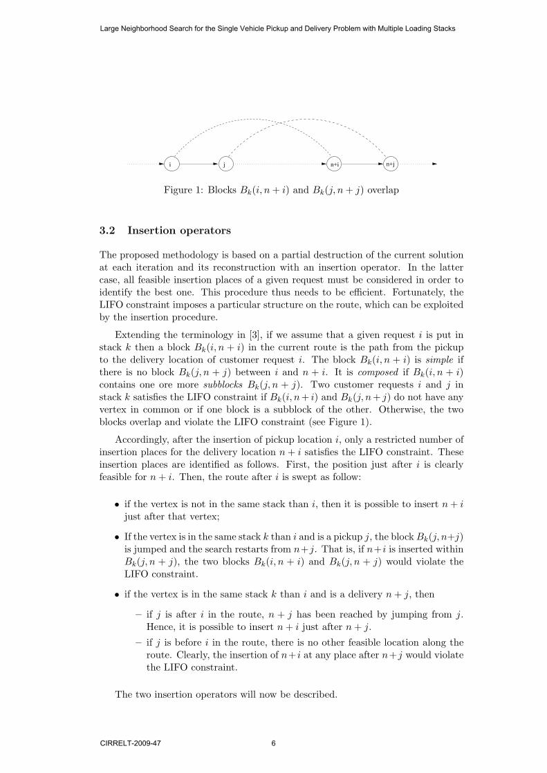
Figure 1: Blocks Bk(i, n + i) and Bk(j, n + j) overlap

3.2 Insertion operators

The proposed methodology is based on a partial destruction of the current solutionat each iteration and its reconstruction with an insertion operator. In the lattercase, all feasible insertion places of a given request must be considered in order toidentify the best one. This procedure thus needs to be efficient. Fortunately, theLIFO constraint imposes a particular structure on the route, which can be exploitedby the insertion procedure.

Extending the terminology in [3], if we assume that a given request i is put instack k then a block Bk(i, n + i) in the current route is the path from the pickupto the delivery location of customer request i. The block Bk(i, n + i) is simple ifthere is no block Bk(j, n + j) between i and n + i. It is composed if Bk(i, n + i)contains one ore more subblocks Bk(j, n + j). Two customer requests i and j instack k satisfies the LIFO constraint if Bk(i, n+ i) and Bk(j, n+ j) do not have anyvertex in common or if one block is a subblock of the other. Otherwise, the twoblocks overlap and violate the LIFO constraint (see Figure 1).

Accordingly, after the insertion of pickup location i, only a restricted number ofinsertion places for the delivery location n + i satisfies the LIFO constraint. Theseinsertion places are identified as follows. First, the position just after i is clearlyfeasible for n + i. Then, the route after i is swept as follow:

• if the vertex is not in the same stack than i, then it is possible to insert n + i

just after that vertex;

• If the vertex is in the same stack k than i and is a pickup j, the block Bk(j, n+j)is jumped and the search restarts from n+j. That is, if n+i is inserted withinBk(j, n + j), the two blocks Bk(i, n + i) and Bk(j, n + j) would violate theLIFO constraint.

• if the vertex is in the same stack k than i and is a delivery n + j, then

– if j is after i in the route, n + j has been reached by jumping from j.Hence, it is possible to insert n + i just after n + j.

– if j is before i in the route, there is no other feasible location along theroute. Clearly, the insertion of n+ i at any place after n+j would violatethe LIFO constraint.

The two insertion operators will now be described.


CIRRELT-2009-47 6

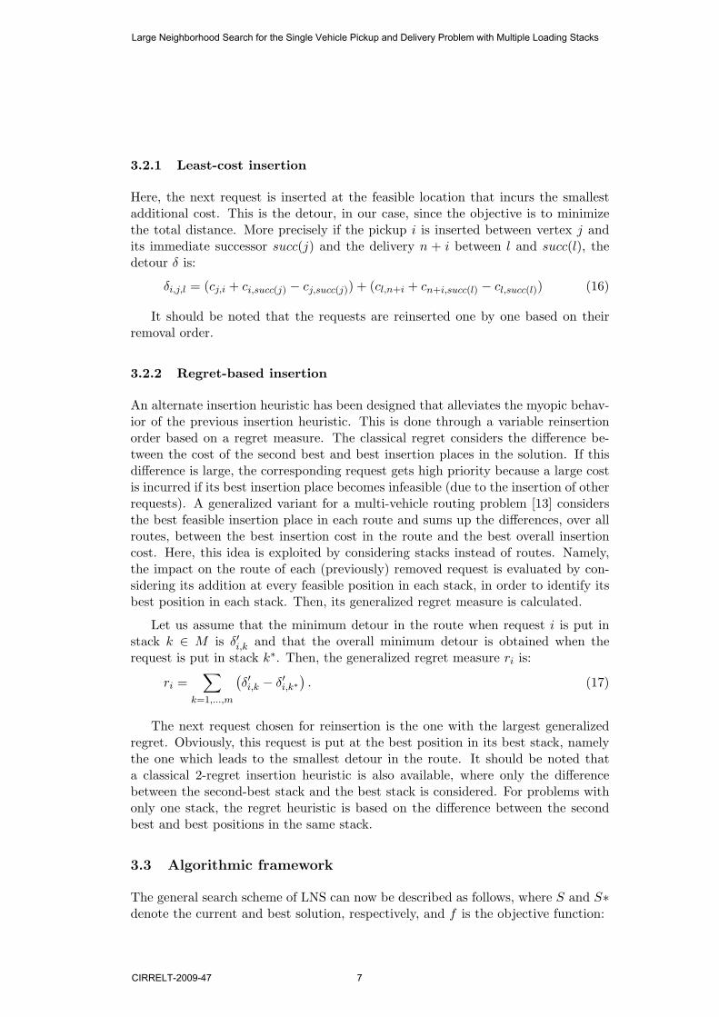
3.2.1 Least-cost insertion

Here, the next request is inserted at the feasible location that incurs the smallestadditional cost. This is the detour, in our case, since the objective is to minimizethe total distance. More precisely if the pickup i is inserted between vertex j andits immediate successor succ(j) and the delivery n + i between l and succ(l), thedetour δ is:

δi,j,l = (cj,i + ci,succ(j) − cj,succ(j)) + (cl,n+i + cn+i,succ(l) − cl,succ(l)) (16)

It should be noted that the requests are reinserted one by one based on theirremoval order.

3.2.2 Regret-based insertion

An alternate insertion heuristic has been designed that alleviates the myopic behav-ior of the previous insertion heuristic. This is done through a variable reinsertionorder based on a regret measure. The classical regret considers the difference be-tween the cost of the second best and best insertion places in the solution. If thisdifference is large, the corresponding request gets high priority because a large costis incurred if its best insertion place becomes infeasible (due to the insertion of otherrequests). A generalized variant for a multi-vehicle routing problem [13] considersthe best feasible insertion place in each route and sums up the differences, over allroutes, between the best insertion cost in the route and the best overall insertioncost. Here, this idea is exploited by considering stacks instead of routes. Namely,the impact on the route of each (previously) removed request is evaluated by con-sidering its addition at every feasible position in each stack, in order to identify itsbest position in each stack. Then, its generalized regret measure is calculated.

Let us assume that the minimum detour in the route when request i is put instack k ∈ M is δ′i,k and that the overall minimum detour is obtained when therequest is put in stack k∗. Then, the generalized regret measure ri is:

ri =∑

k=1,...,m

(

δ′i,k − δ′i,k∗

)

. (17)

The next request chosen for reinsertion is the one with the largest generalizedregret. Obviously, this request is put at the best position in its best stack, namelythe one which leads to the smallest detour in the route. It should be noted thata classical 2-regret insertion heuristic is also available, where only the differencebetween the second-best stack and the best stack is considered. For problems withonly one stack, the regret heuristic is based on the difference between the secondbest and best positions in the same stack.

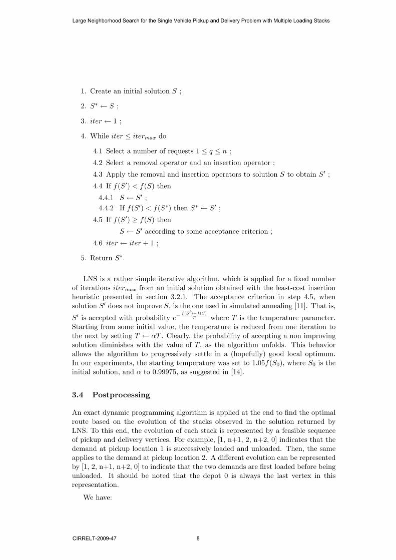
3.3 Algorithmic framework

The general search scheme of LNS can now be described as follows, where S and S∗denote the current and best solution, respectively, and f is the objective function:


CIRRELT-2009-47 7

1. Create an initial solution S ;

2. S∗ ← S ;

3. iter ← 1 ;

4. While iter ≤ itermax do

4.1 Select a number of requests 1 ≤ q ≤ n ;

4.2 Select a removal operator and an insertion operator ;

4.3 Apply the removal and insertion operators to solution S to obtain S′ ;

4.4 If f(S′) < f(S) then

4.4.1 S ← S′ ;

4.4.2 If f(S′) < f(S∗) then S∗ ← S′ ;

4.5 If f(S′) ≥ f(S) then

S ← S′ according to some acceptance criterion ;

4.6 iter ← iter + 1 ;

5. Return S∗.

LNS is a rather simple iterative algorithm, which is applied for a fixed numberof iterations itermax from an initial solution obtained with the least-cost insertionheuristic presented in section 3.2.1. The acceptance criterion in step 4.5, whensolution S′ does not improve S, is the one used in simulated annealing [11]. That is,

S′ is accepted with probability e−f(S′)−f(S)

T where T is the temperature parameter.Starting from some initial value, the temperature is reduced from one iteration tothe next by setting T ← αT . Clearly, the probability of accepting a non improvingsolution diminishes with the value of T , as the algorithm unfolds. This behaviorallows the algorithm to progressively settle in a (hopefully) good local optimum.In our experiments, the starting temperature was set to 1.05f(S0), where S0 is theinitial solution, and α to 0.99975, as suggested in [14].

3.4 Postprocessing

An exact dynamic programming algorithm is applied at the end to find the optimalroute based on the evolution of the stacks observed in the solution returned byLNS. To this end, the evolution of each stack is represented by a feasible sequenceof pickup and delivery vertices. For example, [1, n+1, 2, n+2, 0] indicates that thedemand at pickup location 1 is successively loaded and unloaded. Then, the sameapplies to the demand at pickup location 2. A different evolution can be representedby [1, 2, n+1, n+2, 0] to indicate that the two demands are first loaded before beingunloaded. It should be noted that the depot 0 is always the last vertex in thisrepresentation.

We have:


CIRRELT-2009-47 8

• M = {M1, ..., Mk, ..., Mm}, the set of feasible sequences of pickups and deliv-eries associated with each stack (see the representation above);

• Mk, the sequence of pickups and deliveries associated with stack k, 1 ≤ k ≤ m;

• T = {t1, ..., tk, ..., tm} the set of current positions in the sequences of pickupsand deliveries;

• Mk,tk , the pickup or delivery vertex at position tk in Mk;

• hk(T ) a function that increments the current position in stack k; that is, T

becomes {t1, ..., tk + 1, ..., tm}.

The recurrence relation is then written as follows:

f∗(x, T ) = mink∈M,Mk,tk6=0{cx,Mk,tk

+ f∗(Mk,tk , hk(T ))} if Mk,tk 6= 0 for atleast one k, 1 ≤ k ≤ m,

f∗(x, T ) = cx0 otherwise

At the start, the current route is empty, vertex x is the depot 0 and T indicatesthe first position in each sequence. At each step, a vertex at one of the positionsindicated by T is selected and inserted at the end of the current route. The recur-rence stops when T indicates the last position in each sequence, which correspondsto the depot 0.

4 Computational Results

The experiments reported in this section have been performed on a 2.2 GHz AMDOpteron 275. In the following, the generation of our 1-PDPMS test instances is firstdescribed. Then, different sensitivity analysis experiments are reported, involvingthe number of requests q to be removed and the various removal and insertionoperators. The final results obtained with LNS are then reported. This is followedby a comparison of LNS with state-of-the-art methods on benchmark instances forthe TSPPDL and DTSPMS, which are special cases of the 1-PDPMS.

4.1 1-PDPMS instances

Our 1-PDPMS instances are derived from those for the TSPPDL in [3]. Theseinstances contain between 25 and 751 vertices (including the depot). Three differentclasses were designed: class C1 adds a second stack to the original instances, whilekeeping an infinite capacity for each stack; class C2 contains instances with 2 to 5stacks, a unit demand for every customer request and a capacity constraint on eachstack; class C3 also contains instances with 2 to 5 stacks, but the demand variesbetween 1 and 10 units and the capacity constraint is tighter. Clearly, the degree ofdifficulty increases from class C1 to C3. The characteristics of these instances are


CIRRELT-2009-47 9

Identifier Size C1 C2 C3# Stacks Cap. # Stacks Cap. # Stacks Cap.

brd14051 25 2 ∞ 3 2 3 1651 2 ∞ 3 3 3 1475 2 ∞ 3 4 3 18101 2 ∞ 4 2 4 10251 2 ∞ 3 14 3 28501 2 ∞ 3 20 3 35751 2 ∞ 2 25 2 35

d15112 25 2 ∞ 3 2 3 1251 2 ∞ 4 1 4 1075 2 ∞ 3 4 3 18101 2 ∞ 2 6 2 22251 2 ∞ 2 14 2 28501 2 ∞ 3 20 3 35751 2 ∞ 3 25 3 35

d18512 25 2 ∞ 3 2 3 1251 2 ∞ 5 2 5 1075 2 ∞ 2 4 2 18101 2 ∞ 4 1 4 10251 2 ∞ 3 14 3 28501 2 ∞ 2 5 2 18751 2 ∞ 3 25 3 35

fnl4461 25 2 ∞ 3 2 3 1251 2 ∞ 3 3 3 1475 2 ∞ 5 2 5 13101 2 ∞ 3 6 3 22251 2 ∞ 4 5 4 19501 2 ∞ 2 20 2 35751 2 ∞ 3 25 3 35

nrw1379 25 2 ∞ 2 1 2 1051 2 ∞ 4 2 4 1075 2 ∞ 3 8 3 10101 2 ∞ 2 11 2 10251 2 ∞ 2 6 2 10501 2 ∞ 2 10 2 10751 2 ∞ 3 15 3 10

pr1002 25 2 ∞ 3 1 3 1051 2 ∞ 3 2 3 1475 2 ∞ 4 2 4 10101 2 ∞ 3 4 3 20251 2 ∞ 3 4 3 14501 2 ∞ 3 8 3 25751 2 ∞ 2 8 2 25

Table 1: 1− PDPMS instances


CIRRELT-2009-47 10

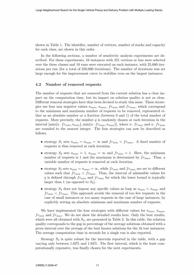
shown in Table 1. The identifier, number of vertices, number of stacks and capacityfor each class, are shown in this order.

In the following sections, a number of sensitivity analysis experiments are de-scribed. For these experiments, 16 instances with 251 vertices or less were selectedover the three classes and 10 runs were executed on each instance, with 25,000 iter-ations per run (for a total of 250,000 iterations). The number of iterations was setlarge enough for the improvement curve to stabilize even on the largest instances.

4.2 Number of removed requests

The number of requests that are removed from the current solution has a clear im-pact on the computation time, but its impact on solution quality is not so clear.Different removal strategies have thus been devised to study this issue. These strate-gies use four non negative values nmin, nmax, frmin and frmax, which correspondto the minimum and maximum number of requests to be removed, represented ei-ther as an absolute number or a fraction (between 0 and 1) of the total number ofrequests. More precisely, the number q is randomly chosen at each iteration in theinterval [min{n · frmin, nmin}, min{n · frmax, nmax}], where n · frmin and n · frmax

are rounded to the nearest integer. The four strategies can now be described asfollows.

• strategy S1 sets nmin = nmax = ∞ and frmin = frmax. A fixed number ofrequests is thus removed at each iteration.

• strategy S2 sets nmin = 1, nmax = ∞ and frmin = 1. Here, the minimumnumber of requests is 1 and the maximum is determined by frmax. Thus, avariable number of requests is removed at each iteration.

• strategy S3 sets nmin = nmax =∞, while frmin and frmax are set to differentvalues such that frmin < frmax. Thus, the interval of admissible values forq is defined through frmin and frmax for which the lower bound is typicallylarger than 1 (as opposed to S2).

• strategy S4 does not impose any specific values as long as nmin < nmax andfrmin < frmax. This approach avoids the removal of too few requests in thecase of small instances or too many requests in the case of large instances, byexplicitly setting an absolute minimum and maximum number of requests.

We have implemented the four strategies with different values for nmin, nmax,frmin and frmax. We do not show the detailed results here. Only the best results,which were all obtained with S4, are presented in Table 2. In this table, the solutionquality corresponds to the gap in percentage of the average solutions obtained with agiven interval over the average of the best known solutions for the 16 test instances.The average computation time in seconds for a single run is also reported.

Strategy S4 is quite robust for the intervals reported in the table, with a gapvarying only between 1.62% and 1.94%. The first interval, which is the least com-putationally expensive, was finally chosen for the next experiments.


CIRRELT-2009-47 11

Test Interval Sol CPU(%) (s)

1 [min{10, 0.15n}, min{35, 0.45n}] 1.85 30.62 [min{15, 0.15n}, min{40, 0.45n}] 1.72 33.03 [min{20, 0.15n}, min{45, 0.45n}] 1.93 35.04 [min{30, 0.15n}, min{50, 0.45n}] 1.86 36.15 [min{10, 0.20n}, min{35, 0.55n}] 1.76 41.26 [min{15, 0.20n}, min{40, 0.55n}] 1.80 46.07 [min{20, 0.20n}, min{45, 0.55n}] 1.94 48.98 [min{30, 0.20n}, min{50, 0.55n}] 1.62 51.19 [min{10, 0.30n}, min{35, 0.60n}] 1.82 53.910 [min{15, 0.30n}, min{40, 0.60n}] 1.69 55.011 [min{20, 0.30n}, min{45, 0.60n}] 1.75 60.012 [min{30, 0.30n}, min{50, 0.60n}] 1.77 64.0

Table 2: Results of strategy S4 with different intervals

Insertion Removal Sol CPU(%) (s)

Least-cost Random 2.59 5.3Distance 2.54 9.0Route 3.67 5.1Stack 2.31 8.9All 2.28 6.9

All minus Route 2.55 7.1

Regret Random 1.79 51.5Distance 1.81 54.4Route 2.94 49.6Stack 1.77 55.1All 1.63 53.0


All Random 1.84 42.5Distance 1.69 45.8Route 3.09 41.6Stack 1.73 46.0All 1.65 43.7


Table 3: Results with different subsets of operators

4.3 Operators

This subsection studies the impact of the various removal and insertion operatorson solution quality. To this end, we consider variants of LNS using only a subsetof operators. As indicated in Table 3, implementations based on only one insertionoperator, either Least-Cost or Regret, or both insertion operators are tested incombination with only one removal operator, with all removal operators or with allremoval operators minus the Route-based operator, which proved to be the worst.

Although the Route-based removal operator is much worse than the other re-moval operators, its inclusion seems to be beneficial (perhaps, by providing a form ofdiversification), as solution quality degrades when it is discarded. The Stack-basedremoval operator alone is quite good and performs well overall when compared withthe other implementations based on a single removal operator. The table also in-


CIRRELT-2009-47 12

LNSClass Size Best Avg CPU

(%) (%) (s)

C1 25 0.00 0.00 0.451 0.00 0.01 2.975 0.00 0.57 9.4101 0.04 0.19 25.1251 0.10 1.11 184.4501 0.00 2.43 519.2751 0.85 2.77 1112.5

C2 25 0.00 0.00 0.451 0.00 0.09 2.975 0.00 0.50 10.3101 0.00 0.46 26.8251 0.00 1.33 182.4501 3.00 4.15 548.0751 2.75 3.56 1126.9

C3 25 0.00 0.00 0.451 0.00 0.19 2.875 0.00 0.93 9.0101 0.13 0.74 25.3251 0.44 3.53 178.0501 0.51 2.47 517.0751 1.43 3.38 938.4

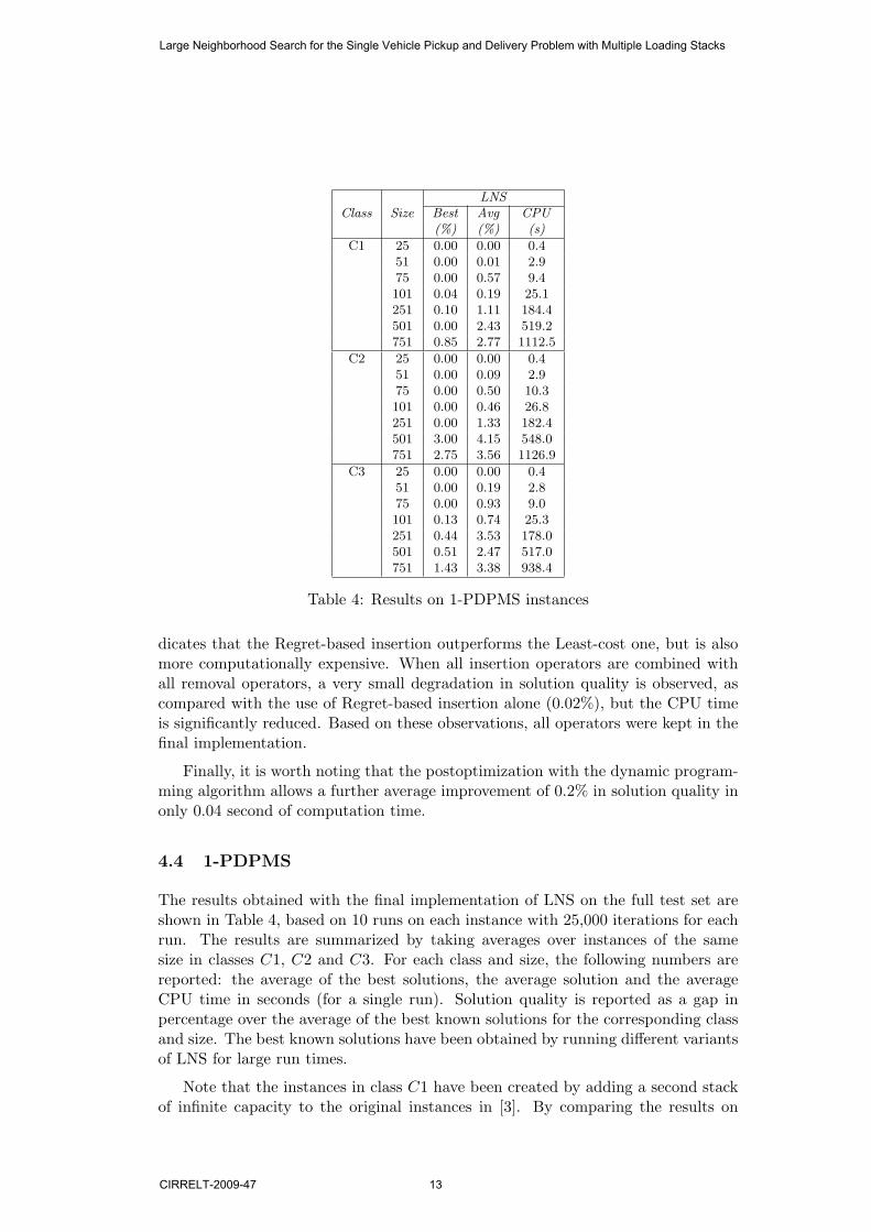
Table 4: Results on 1-PDPMS instances

dicates that the Regret-based insertion outperforms the Least-cost one, but is alsomore computationally expensive. When all insertion operators are combined withall removal operators, a very small degradation in solution quality is observed, ascompared with the use of Regret-based insertion alone (0.02%), but the CPU timeis significantly reduced. Based on these observations, all operators were kept in thefinal implementation.

Finally, it is worth noting that the postoptimization with the dynamic program-ming algorithm allows a further average improvement of 0.2% in solution quality inonly 0.04 second of computation time.

4.4 1-PDPMS

The results obtained with the final implementation of LNS on the full test set areshown in Table 4, based on 10 runs on each instance with 25,000 iterations for eachrun. The results are summarized by taking averages over instances of the samesize in classes C1, C2 and C3. For each class and size, the following numbers arereported: the average of the best solutions, the average solution and the averageCPU time in seconds (for a single run). Solution quality is reported as a gap inpercentage over the average of the best known solutions for the corresponding classand size. The best known solutions have been obtained by running different variantsof LNS for large run times.

Note that the instances in class C1 have been created by adding a second stackof infinite capacity to the original instances in [3]. By comparing the results on


CIRRELT-2009-47 13

class C1 with those reported in [3], we observed an average improvement of 22% intotal distance. This is not a surprise, given the additional flexibility provided bythe second stack.

4.5 TSPPDL

Benchmark instances for the TSPPDL, which is a special case of the 1-PDPMSwhen the vehicle contains a single stack of infinite capacity, are found in [2, 3]. The63 instances in [2] are small because they were designed to test an exact algorithm.This exact algorithm found the optimum on 52 of these instances. A second testset of 42 instances is reported in [3]. These instances range in size from 25 to 751vertices and were designed to test a Variable Neighborhood Search (VNS).

The results on the first test set are shown in Table 5 in the usual format. Whenthe optimum is not known for a given instance, the best known solution, as reportedin [2], is shown in italic. This table shows that LNS found the optimum or bestknown in all cases but one, when the best of 10 runs is considered. It also improvedthe best known solution for the instance nrw1379 with 35 vertices. Even when theaverage of 10 runs is considered, the solutions obtained are only 0.06% over thosereported in [2] with CPU times that do not exceed 1 second.

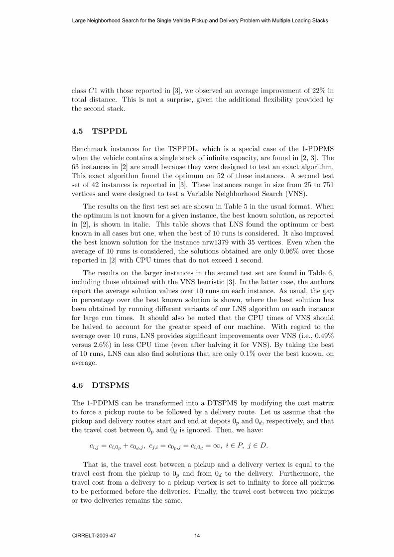
The results on the larger instances in the second test set are found in Table 6,including those obtained with the VNS heuristic [3]. In the latter case, the authorsreport the average solution values over 10 runs on each instance. As usual, the gapin percentage over the best known solution is shown, where the best solution hasbeen obtained by running different variants of our LNS algorithm on each instancefor large run times. It should also be noted that the CPU times of VNS shouldbe halved to account for the greater speed of our machine. With regard to theaverage over 10 runs, LNS provides significant improvements over VNS (i.e., 0.49%versus 2.6%) in less CPU time (even after halving it for VNS). By taking the bestof 10 runs, LNS can also find solutions that are only 0.1% over the best known, onaverage.

4.6 DTSPMS

The 1-PDPMS can be transformed into a DTSPMS by modifying the cost matrixto force a pickup route to be followed by a delivery route. Let us assume that thepickup and delivery routes start and end at depots 0p and 0d, respectively, and thatthe travel cost between 0p and 0d is ignored. Then, we have:

ci,j = ci,0p + c0d,j , cj,i = c0p,j = ci,0d=∞, i ∈ P, j ∈ D.

That is, the travel cost between a pickup and a delivery vertex is equal to thetravel cost from the pickup to 0p and from 0d to the delivery. Furthermore, thetravel cost from a delivery to a pickup vertex is set to infinity to force all pickupsto be performed before the deliveries. Finally, the travel cost between two pickupsor two deliveries remains the same.


CIRRELT-2009-47 14

LNSInstance Size Optimum Best Avg CPU

(%) (%) (s)

a280 19 402 0.00 0.00 0.223 468 0.00 0.00 0.227 505 0.00 0.00 0.331 560 0.00 0.00 0.435 647 0.00 0.00 0.639 691 0.00 0.00 0.843 752 0.00 0.00 1.0

att532 19 4250 0.00 0.00 0.223 5038 0.00 0.00 0.227 5800 0.00 0.00 0.331 6173 0.00 0.00 0.435 6361 0.00 0.00 0.639 6725 0.00 0.00 0.843 10714 0.00 0.05 1.0

brd14051 19 4555 0.00 0.00 0.223 4655 1.29 1.29 0.227 4936 0.00 0.00 0.331 5186 0.00 0.00 0.435 5196 0.00 0.00 0.639 5629 0.00 0.00 0.743 5719 0.00 0.00 1.0

d15112 19 76203 0.00 0.00 0.223 88272 0.00 0.16 0.227 93158 0.00 0.25 0.331 109166 0.00 0.22 0.535 115554 0.00 0.00 0.639 119863 0.00 0.00 0.843 128798 0.00 0.00 1.0

d18512 19 4446 0.00 0.00 0.223 4658 0.00 0.00 0.227 4704 0.00 0.00 0.331 5120 0.00 0.00 0.535 5186 0.00 0.00 0.639 5419 0.00 0.00 0.743 5634 0.00 0.00 1.0

fnl4461 19 1866 0.00 0.00 0.223 2067 0.00 0.00 0.227 2483 0.00 0.00 0.331 2672 0.00 0.00 0.435 2852 0.00 0.00 0.639 3109 0.00 0.00 0.743 3269 0.00 0.00 1.0


CIRRELT-2009-47 15

LNSInstance Size Optimum Best Avg CPU

(%) (%) (s)

nrw1379 19 2691 0.00 0.00 0.223 2919 0.00 0.00 0.227 3366 0.00 0.00 0.331 3554 0.00 0.00 0.535 3652 -0.22 -0.22 0.639 4002 0.00 0.00 0.843 4282 0.00 0.00 1.0

pr1002 19 12947 0.00 0.00 0.223 13872 0.00 0.00 0.227 15566 0.00 0.00 0.331 16255 0.00 0.00 0.435 17564 0.00 0.00 0.639 18862 0.00 0.00 0.743 20173 0.00 0.00 1.0

ts225 19 21000 0.00 0.00 0.223 25000 0.00 0.00 0.227 32395 0.00 0.00 0.331 33395 0.00 1.65 0.535 36703 0.00 0.13 0.639 39395 0.00 0.00 0.843 43082 0.00 0.00 1.0

Avg 0.02 0.06 0.5

Table 5: Results on the first test set of Carrabs, Cerruli and Cordeau

A test set with 60 randomly generated Euclidean DTSPMS instances is reportedin [12], where the distances have been rounded to the nearest integer. More precisely,there are 20 instances with 12, 33 and 66 customer requests (i.e, 26, 68 and 132vertices, including the two depots). All customer requests have a unit demand. Ineach instance, the vehicle contains three stacks and the capacity of each stack is onethird of the total demand. The optimal solutions are known for the instances with12 requests, but for the larger ones, the best known solutions have been obtainedby Petersen and Madsen [12] after multiple 2-hour runs of their algorithm on eachinstance. Solution quality is thus represented as the gap in percentage with eitherthe optimal solutions or the best known solutions produced by Petersen and Madsen.

In Tables 7, 8 and 9, the solutions obtained with our algorithms are comparedwith the solutions of Petersen and Madsen for the instances with 12, 33 and 66requests, respectively. The algorithm of Madsen and Petersen is a combination ofa large neighborhood search (using insertion and removal operators different fromours) and a local search based on vertex exchanges. In the tables, Short and Long

refer to two different calibrations of this algorithm for short (10 seconds) and long (3minutes) runs. It should be noted that the machine and programming language usedin our implementation lead to running times that are about 3 times faster than thoseof Petersen and Madsen. Accordingly, Short and Long would approximately run for3 seconds and 1 minute, respectively, on our machine. The solutions reported byFelipe et al. in [4], obtained with a variable neighborhood search approach, are alsoshown in Tables 8 and 9 (the authors do not provide detailed results on each instance


CIRRELT-2009-47 16

VNS LNSInstance Size Avg CPU Best Avg CPU

(%) (s) (%) (%) (s)

fnl4461 25 0.00 0.0 0.00 0.00 0.351 0.00 0.1 0.00 0.00 1.575 2.20 0.2 0.00 0.00 4.6101 3.78 0.7 0.00 0.32 10.5251 2.51 23.9 0.00 0.66 71.5501 3.95 458.6 0.00 1.29 215.1751 3.53 2172.5 0.00 0.57 532.8

brd14051 25 0.22 0.0 0.00 0.00 0.351 0.30 0.1 0.00 0.00 1.575 1.07 0.3 0.00 0.00 4.0101 2.82 0.7 0.00 0.01 10.2251 8.44 36.7 0.00 1.83 72.0501 5.56 478.7 0.89 1.68 213.2751 4.63 2169.8 0.75 1.32 482.8

d15112 25 0.00 0.0 0.00 0.00 0.351 1.03 0.0 0.00 0.00 1.475 1.20 0.2 0.00 0.00 4.5101 4.41 0.5 0.00 0.36 10.8251 4.80 24.6 0.00 0.94 73.0501 3.01 385.9 0.03 1.03 218.1751 2.22 1968.6 0.00 0.83 465.8

d18512 25 0.24 0.0 0.00 0.00 0.351 0.85 0.1 0.00 0.00 1.475 1.77 0.2 0.00 0.00 3.9101 0.88 0.5 0.00 0.00 10.2251 6.94 32.9 0.15 0.99 70.2501 5.65 486.0 0.00 0.71 243.4751 3.58 2508.5 0.51 0.86 576.2

nrw1379 25 0.09 0.0 0.00 0.00 0.351 0.79 0.1 0.00 0.00 1.475 0.50 0.2 0.00 0.00 4.5101 3.88 0.5 0.00 0.34 9.9251 5.54 24.5 0.00 0.89 72.3501 3.60 380.1 0.22 1.20 218.9751 2.23 2447.1 0.00 0.74 516.4

pr1002 25 0.00 0.0 0.00 0.00 0.351 0.81 0.1 0.00 0.00 1.575 0.67 0.3 0.21 0.22 4.4101 3.44 0.8 0.00 0.19 10.8251 5.86 31.3 1.19 1.87 68.6501 3.57 471.9 0.00 1.25 213.5751 2.80 2785.4 0.04 0.49 500.7

Avg 2.60 402.2 0.10 0.49 117.2

Table 6: Results on the second test set of Carrabs, Cordeau and Laporte


CIRRELT-2009-47 17

for the test set with 12 requests). Average solutions, over 3 runs, are reported after10 seconds and 3 minutes of computation times. No CPU time adjustment is neededhere, because the machine used by Felipe et al. is similar to ours.

Table 7 provides comparisons with the optimum on the small 12-request in-stances. In the case of Petersen and Madsen, the results are averages of three runs,and the optimum has been found in all cases. The average solution value of LNS is0.08% over the optimum, but the best of 10 runs is always optimal. These 10 runsexecute in 10 · 0.5 = 5 seconds which is comparable to the Short runs of Petersenand Madsen. It should be noted that Felipe et al. report an average gap (over threeruns on each instance) of 0.2%, in only one second of CPU time. They did not findthe optimum on two instances.

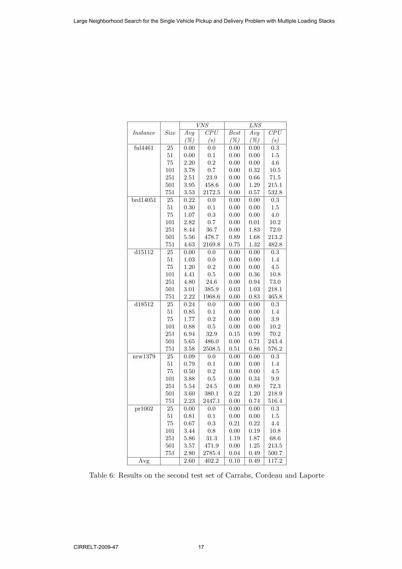
Tables 8 and 9 show the results for the larger instances with 33 and 66 customerrequests. On the instances with 33 requests, the average run of LNS is 0.65% overthe best known using only 11.1 seconds of CPU time. This is an improvement overthe (single) Long run of Petersen and Madsen which provides a solution which is1% over the best known in 1 minute of equivalent CPU time. When the best of 10runs is considered, LNS gets as close as 0.05% over the best known in 10 · 11.1 =111 seconds. The results produced by LNS are very similar to those obtained byFelipe et al. who report average gaps of 0.65% after 10 seconds and 0.05% after 3minutes. On the instances with 66 requests, LNS is 2.76% over the best known onaverage in less than 2 minutes of CPU time. This is better than the (single) Long

run of Petersen and Madsen which is 8% over the best known, admittedly after only1 minute of equivalent CPU time. By reducing the number of iterations of LNS from25,000 to 12,500, to obtain runs of approximately 1 minute, the average solution ofLNS remains at 3.28% over the best known, which is still better than Petersen andMadsen. The average gap of 2.76% in less than 2 minutes is also better than theLong run of Felipe et al. which is 3.2% over the best known after 3 minutes of CPUtime. When the best of 10 runs is considered, LNS gets solutions that are 1.17%over the best known, on average. Furthermore, a best known solution was found oninstance R05-66.

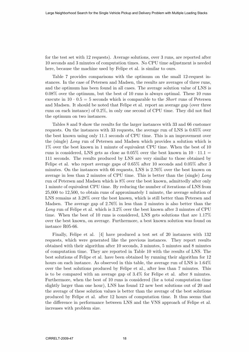
Finally, Felipe et al. [4] have produced a test set of 20 instances with 132requests, which were generated like the previous instances. They report resultsobtained with their algorithm after 10 seconds, 3 minutes, 5 minutes and 8 minutesof computation time. They are reported in Table 10 with the results of LNS. Thebest solutions of Felipe et al. have been obtained by running their algorithm for 12hours on each instance. As observed in this table, the average run of LNS is 1.64%over the best solutions produced by Felipe et al., after less than 7 minutes. Thisis to be compared with an average gap of 3.4% for Felipe et al. after 8 minutes.Furthermore, when the best of 10 runs is considered (for a total computation timeslightly larger than one hour), LNS has found 12 new best solutions out of 20 andthe average of these solution values is better than the average of the best solutionsproduced by Felipe et al. after 12 hours of computation time. It thus seems thatthe difference in performance between LNS and the VNS approach of Felipe et al.increases with problem size.


CIRRELT-2009-47 18

Petersen & Madsen LNSInstance Optimal Short Long Best Avg CPU

(%) (%) (%) (%) (s)

R00-12 694 0 0 0.00 0.52 0.5R01-12 710 0 0 0.00 0.31 0.5R02-12 606 0 0 0.00 0.00 0.5R03-12 680 0 0 0.00 0.00 0.5R04-12 607 0 0 0.00 0.00 0.5R05-12 567 0 0 0.00 0.00 0.5R06-12 747 0 0 0.00 0.00 0.5R07-12 557 0 0 0.00 0.00 0.5R08-12 690 0 0 0.00 0.00 0.5R09-12 669 0 0 0.00 0.00 0.5

R10-12 633 0 0 0.00 0.00 0.5R11-12 591 0 0 0.00 0.00 0.5R12-12 722 0 0 0.00 0.17 0.5R13-12 664 0 0 0.00 0.00 0.5R14-12 650 0 0 0.00 0.26 0.5R15-12 595 0 0 0.00 0.27 0.5R16-12 577 0 0 0.00 0.00 0.5R17-12 737 0 0 0.00 0.00 0.5R18-12 724 0 0 0.00 0.01 0.5R19-12 753 0 0 0.00 0.16 0.5

Avg 0 0 0.00 0.08 0.5

Table 7: Results on the DTSPMS instances of Petersen and Madsen with 12 requests

Petersen & Madsen Felipe et al. LNSInstance Best Short Long Short Long Best Avg CPU

(%) (%) (%) (%) (%) (%) (s)

R00 1063 4 1 0.8 0.0 0.00 0.57 10.6R01 1032 4 1 0.8 0.0 0.00 0.24 10.7R02 1065 4 1 0.8 0.0 0.00 0.25 10.7R03 1100 6 1 0.0 0.0 0.00 1.00 11.2R04 1052 5 2 0.5 0.0 0.00 1.14 11.2R05 1008 3 1 2.2 0.0 0.00 0.84 11.0R06 1110 6 2 0.0 0.0 0.00 0.31 11.2R07 1105 5 1 0.4 0.0 0.36 0.90 11.1R08 1109 4 1 0.0 0.0 0.00 0.55 11.1R09 1091 4 1 0.0 0.0 0.00 0.54 11.1

R10 1016 5 0 0.0 0.0 0.00 0.00 11.3R11 1001 6 1 0.0 0.0 0.00 0.60 11.1R12 1109 4 1 0.2 0.0 0.18 0.74 11.1R13 1084 4 1 0.0 0.0 0.00 0.62 11.0R14 1034 3 0 1.7 0.0 0.00 0.69 11.1R15 1142 4 1 1.4 0.0 0.26 1.02 11.3R16 1093 2 0 0.0 0.0 0.00 0.15 11.2R17 1073 4 0 0.9 0.0 0.00 0.57 10.9R18 1118 5 1 2.8 0.7 0.00 1.33 11.3R19 1089 3 1 0.6 0.2 0.28 0.91 11.2

Avg 4 1 0.66 0.05 0.05 0.65 11.1



CIRRELT-2009-47 19

Petersen & Madsen Felipe et al. LNSInstance Best Short Long Short Long Best Avg CPU

(%) (%) (%) (%) (%) (%) (s)

R00-66 1594 19 7 3.8 3.1 0.31 2.65 108.9R01-66 1600 20 8 6.4 4.3 1.25 3.09 110.1R02-66 1576 20 12 7.7 6.2 3.55 4.90 109.6R03-66 1631 14 6 5.9 2.5 0.67 2.02 111.3R04-66 1611 18 9 7.7 2.9 1.49 3.16 111.4R05-66 1528 18 7 6.9 3.3 -0.13 1.30 112.1R06-66 1651 17 7 10.5 3.6 0.42 2.13 111.5R07-66 1653 17 8 6.4 1.0 1.21 3.02 111.6R08-66 1607 18 7 11.1 3.4 0.62 3.04 111.6R09-66 1598 18 8 8.6 3.1 2.07 2.78 112.1

R10-66 1702 17 9 7.8 3.9 0.59 1.77 112.4R11-66 1575 19 8 6.7 5.3 0.44 2.98 111.9R12-66 1652 19 10 6.0 2.2 0.30 1.96 112.4R13-66 1617 19 10 8.7 2.5 1.98 3.21 111.6R14-66 1611 21 9 6.6 1.4 0.56 2.59 111.7R15-66 1608 19 10 6.5 1.9 1.31 2.20 111.2R16-66 1725 16 7 8.2 2.6 0.87 2.07 111.8R17-66 1627 21 10 7.5 5.1 2.03 3.34 112.0R18-66 1671 18 8 6.5 2.3 1.97 3.88 112.5R19-66 1635 17 9 5.2 2.9 1.83 3.13 112.5

Avg 18 8 7.2 3.2 1.17 2.76 111.5


Felipe et al. LNSInstance Best 10s 3min 5min 8min Best Best Avg CPU

(%) (%) (%) (%) (%) (%) (s)

R00-132 2591 15.7 6.6 6.3 3.8 2590 -0.04 2.57 400.4R01-132 2645 16.7 5.4 4.2 4.5 2650 0.19 2.14 403.8R02-132 2639 13.9 5.2 4.6 3.1 2679 1.52 2.97 401.1R03-132 2752 12.4 3.2 4.2 1.7 2698 -1.96 0.65 398.7R04-132 2603 13.1 4.6 3.0 2.9 2590 -0.50 0.41 405.7R05-132 2616 15.8 5.7 4.7 4.7 2651 1.34 2.27 401.2R06-132 2576 16.0 7.1 4.6 4.9 2579 0.12 1.93 403.2R07-132 2615 14.7 7.5 4.8 3.6 2559 -2.14 1.00 401.2R08-132 2638 14.3 5.3 4.6 3.4 2636 -0.08 1.71 402.8R09-132 2554 13.6 3.5 2.5 1.3 2499 -2.15 -0.50 399.8

R10-132 2646 19.0 6.4 3.7 3.6 2663 0.64 1.92 400.1R11-132 2632 13.3 4.6 5.2 2.7 2621 -0.42 1.77 401.8R12-132 2555 18.5 6.8 5.3 5.4 2544 -0.43 2.56 401.5R13-132 2659 15.7 5.0 3.3 2.1 2664 0.19 1.76 404.2R14-132 2605 14.0 3.7 2.5 2.7 2568 -1.42 1.13 403.5R15-132 2626 18.5 5.3 5.4 3.8 2634 0.30 1.75 402.1R16-132 2534 16.0 6.7 4.5 4.6 2585 2.01 3.30 400.4R17-132 2569 14.2 4.6 4.3 3.5 2559 -0.39 1.58 402.7R18-132 2652 15.1 3.5 2.0 1.9 2628 -0.90 0.66 402.3R19-132 2644 16.0 4.2 4.6 2.8 2624 -0.76 1.31 401.6

Avg 15.3 5.3 4.2 3.4 -0.24 1.64 401.9

Table 10: Results on the DTSPMS instances of Felipe et al. with 132 requests


CIRRELT-2009-47 20

5 Conclusion

This paper has described a large neighborhood search which is both efficient andeffective for solving the 1-PDPMS. This is also true for special cases of this problem,like the TSPPDL and DTSPMS, as empirically demonstrated through comparisonswith state-of-the-art methods on different sets of benchmark instances. Building onthese results, our aim is now to address the more challenging multi-vehicle extensionof the problem.

Acknowledgments. Financial support for this work was provided by the CanadianNatural Sciences and Engineering Research Council (NSERC). This support is grate-fully acknowledged.

References

[1] Ahuja R.K., Ergun O., Orlin J.B., Punnen A.P., “A Survey of Very Large-ScaleNeighborhood Search Techniques”, Discrete Applied Mathematics 123, 75–102,2002.

[2] Carrabs F., Cerulli R., Cordeau J.-F., “An Additive Branch-and-Bound Algo-rithm for the Pickup and Delivery Traveling Salesman Problem with LIFO orFIFO Loading”, INFOR 45, 223-238, 2007.

[3] Carrabs F., Cordeau J.-F., Laporte G., “Variable Neighborhood Search forthe Pickup and Delivery Traveling Salesman Problem with LIFO Loading”,INFORMS Journal on Computing 19, 618-632, 2007.

[4] Felipe A., Ortuno M.T., Tirado G., “The Double Traveling Salesman Problemwith Multiple Stacks: A Variable Neighborhood Search Approach”, Computers

& Operations Research 36, 2983-2993, 2009.

[5] Doerner K.F., Fuellerer G., Gronalt M., Hartl R.F., Iori M., “Metaheuristicsfor the Vehicle Routing Problem with Loading Constraints”, Networks 49, 294–307, 2007.

[6] Fuellerer G., Doerner K.F., Hartl R.F., Iori M., “Ant Colony Optimizationfor the Two-Dimensional Loading Vehicle Routing Problem”, Computers &

Operations Research 36, 655-673, 2009.

[7] Fuellerer G., Doerner K.F., Hartl R.F., Iori M., “Metaheuristics for VehicleRouting Problems with Three-Dimensional Loading Constraints”, European

Journal of Operational Research, forthcoming, 2009.

[8] Gendreau M., Iori M., Laporte G., Martello S., “A Tabu Search Algorithm for aRouting and Container Loading Problem”, Transportation Science 40, 342-350,2006.


CIRRELT-2009-47 21

[9] Gendreau M., Iori M., Laporte G., Martello S., “A Tabu Search Heuristicfor the Vehicle Routing Problem with Two-Dimensional Loading Constraints”,Networks 51, 4-18, 2008.

[10] Iori M., Salazar-Gonzalez J.-J., Vigo D., “An Exact Approach for the VehicleRouting Problem with Two-Dimensional Loading Constraints”, Transportation

Science 41, 253–264, 2007.

[11] Kirkpatrick S., Gelatt Jr. C.D., Vecchi M.P., “Optimization by Simulated An-nealing”, Science 220, 671–680, 1983.

[12] Petersen H.L., Madsen O.B.G., “The Double Traveling Salesman Problem withMultiple Stacks - Formulation and Heuristic Solution Approaches”, European

Journal of Operational Research 198, 139–147, 2009.

[13] Potvin J.-Y., Rousseau J.-M., “An Exchange Heuristic for Routing Problemswith Time Windows”, Journal of the Operational Research Society 46, 1433–1446, 1995.

[14] Ropke S., Pisinger D., “An Adaptive Large Neighborhood Search Heuristic forthe Pickup and Delivery Problem with Time Windows”, Transportation Science

40, 455–472, 2006.

[15] Schrimpf G., Schneider J., Stamm-Wilbrandt H., Dueck G., “Record Break-ing Optimization Results using the Ruin and Recreate Principle”, Journal of

Computational Physics 159, 139–171, 2000.

[16] Shaw P., “Using Constraint Programming and Local Search Methods to solveVehicle Routing Problems”, Proceedings of the Fourth International Conference

on Principles and Practice of Constraint Programming, M. Maher and J.-F.Puget eds., Lecture Notes in Computer Science 1520, Springer-Verlag, Berlin,417–431, 1998.


CIRRELT-2009-47 22

large neighborhood search for the single vehicle pickup and

Documents