large scale machine learning in the real world · large scale machine learning in the real world...

Large Scale Machine Learning in the Real World

LÉON BOTTOU

PART 1 – PAID SEARCH

1

1. Ads

2

TV

Advertisement primer

Sale!

Paid search

Display ads

Advertisement opportunities

3

Paid search

• The most “effective” online ads are those displayed on search engines.

• How to choose which ads to display where?

4

The game

User Advertiser

QueriesAds& Bids

AdsPrices

Publisher

• Designs ad messages• Selects ad opportunities

(keywords and match criteria)

• Places a bid(maximum price for a click)

1

In general, Paid search advertisers pay when the user clicks on their ad.

(there are other payment models, per impression, per action, etc.)

5

The game

• Revealsinterests with a search query

Advertiser

QueriesAds& Bids

AdsPrices

Publisher

2

Users

6

The game

User Advertiser

QueriesAds& Bids

AdsPrices

Publisher

• Computes search results• Determines which ads to

display (and where!)• Determines price per click

3

7

The game

• May click on a relevant ad and jump to the advertiser site

• Triggering a payment from the advertiser to the publisher.

Advertiser

QueriesAds& Bids

AdsPrices

Publisher

4

User

Clicks

8

Self interest

User

Advertiser

Publisher

• Expects results that satisfy her interests• Possibly by initiating business with an advertiser• Future engagement depends on her satisfaction….

• Expects to receive potential customers• Expects to recover clicks costs from resulting business• Return on investment impacts future ads and bids…

• Expects click money• Learns which ads work from past data.• In order to preserve future gains, publishers must ensure

the continued satisfaction of users and advertisers.(this changes everything!)

9

Second order effects

Users Advertisers

QueriesAds& Bids

Ads Prices

Clicks (and consequences)

ADVERTISER FEEDBACK LOOP

USER FEEDBACK

LOOP

Publisher

10

AuctionsSetup• Seller has an object to sell.

• Each buyer values the object differently.

• Each buyer knows the auction mechanism and places a bid.

• Auction mechanism determines who gets the object and how much he pays.

Notes- The auction outcomes are functions of the bids.

- Buyer bids according to his value and his beliefs about other buyers values.

- The value of whoever gets the object is the size of the pie.

- The payment from the buyer to the seller then splits the pie.

Which mechanism works best for the seller?

11

AuctionsA first auction mechanism

“The highest bidder receives the object and pays his bid.”

Buyers should bid less than their value.o If they bid their value, their surplus is zero in all cases.o If they bid more, they may get the object with a negative surplus.o If they bid less, they trade a chance to lose the object for a chance to pay less.

The object may not go to the buyer who values it most.

The expected pie is smaller and the expected buyer surplus is larger. This cannot be good for the seller.

The object may sell for less than the seller’s value. Can use a reserve price, that is, an additional bid entered by the seller.

12

AuctionsA second auction mechanism

“The highest bidder receives the object and pays the second highest bid.”

Buyers now should bid their value (“truthful mechanism”)

o Overbidding buyers may get the object with negative surplus.

o Underbidding buyers will not pay less if they get the object. On the other hand, they may see the object sold to another buyer for less than their value, losing the opportunity to have a positive surplus.

Unless a buyer is certain that no other buyer will bid above a level smaller than his value, the buyer best interest is to bid his value, regardless of his exact beliefs.

The object always goes to the buyer who values it most.

The object may still sell for less than the seller’s value.

13

AuctionsA third auction mechanism

“The seller announces a reserve price which works like an additional bid. - If the highest bid is the reserve price, the seller keeps the object. - Otherwise the highest bidder receives the object and pays the second highest bid.”

Buyers should still bid their value (“truthful mechanism”)

But the seller should set a reserve price that is higher than his value!o He trades the risk of not selling for the chance to get more than his value.

o Therefore the object may not sell even though a buyer values it more than the seller.This in fact makes the pie smaller in a manner that benefits the seller.

Under mild assumptions, this is the optimal mechanism for the seller.o For the correct value of the reserve price, of course…

14

Ad placement auctionsMapping auction theory to ad placement• The publisher is the seller (he receives bids)

• The advertisers are the buyers (they place bids)

• What about click decisions made by the user?

• What is the “object” exactly?

Click probabilitiesThe click probabilities (𝑞1, … , 𝑞𝑘) of the eligible ads (𝑎1, … , 𝑎𝑘) depend

• on the context 𝑥, that is, the query, the user, the session, the weather…

• on the ad messages themselves (𝑎1, … , 𝑎𝑘),

• on the positions (𝑝1, … , 𝑝𝑘) chosen by the publisher,

• but do not depend on the bids (𝑏1, … , 𝑏𝑘).

15

Ad placement auctions

One of the many ways to view ad placement auctions…

• The auction mechanism specifieso The probability that each competing advertiser gets a click (the object).

o The expected price paid by each competing advertiser.

• There is an optimal mechanism (Myerson, 1981).

o The placement (𝑝1, … , 𝑝𝑘) maximizes 𝑖𝑏𝑖× 𝑞𝑖(𝑥, 𝒂, 𝒑) subject to reserves.

o The prices are determined by the Vickrey-Clarke-Groves (VCG) rule,a nontrivial generalization of the second price rule.

• See also (Varian, 2007; Edelman et al., 2007)

16

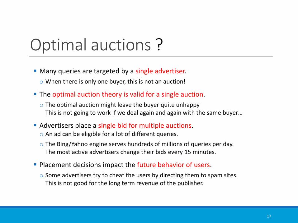
Optimal auctions ?

Many queries are targeted by a single advertiser.

o When there is only one buyer, this is not an auction!

The optimal auction theory is valid for a single auction.

o The optimal auction might leave the buyer quite unhappyThis is not going to work if we deal again and again with the same buyer…

Advertisers place a single bid for multiple auctions.o An ad can be eligible for a lot of different queries.

o The Bing/Yahoo engine serves hundreds of millions of queries per day.The most active advertisers change their bids every 15 minutes.

Placement decisions impact the future behavior of users.

o Some advertisers try to cheat the users by directing them to spam sites.This is not good for the long term revenue of the publisher.

17

How it really worksThe following mechanism is the result of history.This is what the advertisers expect. Changing it is hard!

1. Publisher selects eligible ads (𝑎1, … , 𝑎𝑘) for the query 𝑥.

2. Publisher computes click scores 𝑞𝑖 and rank scores 𝑟𝑖

𝑞𝑖 𝑥, 𝑎𝑖 , 𝑝𝑖 = 𝛾 𝑥, 𝑝𝑖 × 𝛽 𝑥, 𝑎𝑖 𝑟𝑖 𝑥, 𝑎𝑖 = 𝑏𝑖 × 𝛽(𝑥, 𝑎𝑖)

3. Publisher greedily assigns ads with the largest rank scores to the best available positions, until reaching a predefined reserve score

4. Generalized second price (GSP): advertiser pays the smallest bid that would have guaranteed the same placement.

Position effect Ad effect Ad effectBid

18

The ugly truth2. Publisher computes click scores 𝑞𝑖 and rank scores 𝑟𝑖

𝑞𝑖 𝑥, 𝑎𝑖 , 𝑝𝑖 = 𝛾 𝑥, 𝑝𝑖 × 𝛽 𝑥, 𝑎𝑖 𝑟𝑖 𝑥, 𝑎𝑖 = 𝑏𝑖 × 𝛽(𝑥, 𝑎𝑖)

4. Generalized second price.

No longer a pure click probability. Secret ingredients attempt to represent user satisfaction.

The auction is not truthful because GSP is not VCG.

Furthermore, additional ingredients give discounts for

certain auctions.

I do not understand the combined effects of all these adjustments.I have never met anyone who could explain them to me.

19

Logs(TB/day)

The plumbingSearch engine

Queries≈ 108/day

Advertisers

Real time ad placement engine

Selection Scores Auction

Ads (≈109)

Models(GB)

Params(100s)

ExperimentsTrainingAccounting

Offline computing platform

20

2. Experimentation

21

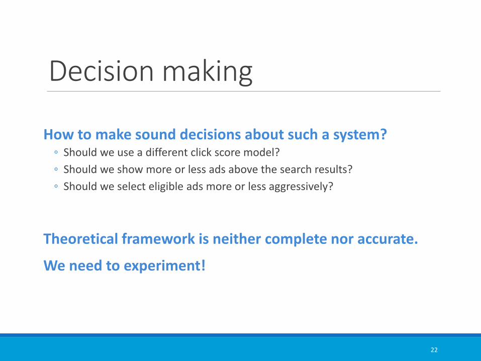
Decision making

How to make sound decisions about such a system?◦ Should we use a different click score model?

◦ Should we show more or less ads above the search results?

◦ Should we select eligible ads more or less aggressively?

Theoretical framework is neither complete nor accurate.

We need to experiment!

22

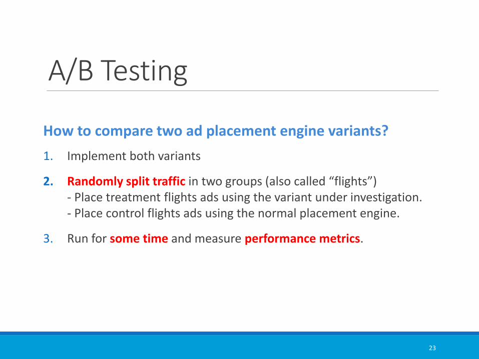
A/B Testing

How to compare two ad placement engine variants?

1. Implement both variants

2. Randomly split traffic in two groups (also called “flights”)- Place treatment flights ads using the variant under investigation.- Place control flights ads using the normal placement engine.

3. Run for some time and measure performance metrics.

23

Performance metricsFirst order performance metrics Average number of ads shown per page

Average number of mainline ads per page

Average number of ad clicks per page

Average revenue per page (RPM)

mainline sidebar

Should we just optimize RPM?

Showing lots of mainline ads improves RPM.Users would quickly go away!

Increasing the reserve prices also improves RPM. Advertisers would quickly go away!

24

Performance metrics

First order performance metrics Average number of ads shown per page

Average number of mainline ads per page

Average number of ad clicks per page

Average revenue per page (RPM)

Average relevance score estimated by human labelers

Average number of bid-weighted ad clicks per page

…

Monitor heuristic indicators of user fatigue

Monitor heuristic indicators of advertiser value

25

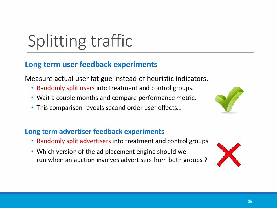
Splitting trafficLong term user feedback experiments

Measure actual user fatigue instead of heuristic indicators.• Randomly split users into treatment and control groups.

• Wait a couple months and compare performance metric.

• This comparison reveals second order user effects…

Long term advertiser feedback experiments• Randomly split advertisers into treatment and control groups

• Which version of the ad placement engine should we run when an auction involves advertisers from both groups ?

26

Significance

Central Limit Theorem

𝑌 =1

𝑛 𝑦𝑖 𝑌 − 𝑌 ~ 𝒩 0,

𝜎

𝑛

Not significant Significant

27

Variance reduction

Hourly average click yield for treatment and control

Daily effects increases the variance of both

treatment and control.

𝑌 −1

𝑛 𝑦𝑖 ~ 𝒩 0,

𝜎

𝑛

Daily effects affect treatment and control in similar ways! Can we subtract them?

28

Variance reduction

• Treatment estimate 𝑌∗ ≈ 𝑌∗ =1

|𝑇| 𝑖∈𝑇 𝑦𝑖

• Control estimate 𝑌 ≈ 𝑌 =1

|𝐶| 𝑖∈𝐶 𝑦𝑖

• Predictor 𝜁 𝑋 tries to estimate 𝑌 on the basis of solely the context 𝑋.

• Then 𝑌∗−𝑌 = 𝑌∗ − 𝜁 𝑋 − 𝑌 − 𝜁 𝑋

≈1

|𝑇| 𝑖∈𝑇 𝑦𝑖 − 𝜁 𝑥𝑖 −

1

|𝐶| 𝑖∈𝐶 𝑦𝑖 − 𝜁 𝑥𝑖

This is true regardless of the predictor quality.

But if it is any good, var 𝑌 − 𝜁 𝑋 < var[𝑌], and

29

Problems with A/B testing

• No single decision criterion

o Because of complex second order effects.

• Requires full implementation of treatment.

• Must wait two weeks for significant results.

o Impractical for the early development of new ideas.

o Cannot drive learning algorithms.

• Experimentation is limited by total traffic.

o Hundreds of experiments are running at the same time.

o Overlapped experiments.

30

3. Learning

31

End-to-end learningIdeally we should train at the system level

“Train all aspects of the system to maximize a well defined objective function.”

Requirements

• The objective function must be correct.

we get what we ask for ( only that and all of it ! )

hard to debug

• Learning impacts global system architecture.

this point is difficult to make.

32

Learning as a component

Train a component of the system• Convenient to manage teams.

• Example: train a click prediction module.

“ If the click prediction guys produce good probability estimates,the auction guys will know what to do…”

• Reproducing a software development pattern.

Machine learning is not like software development

• Machine learning is about the estimation error.How will they affect the other components of the system?

33

Click prediction and auctionsOptimal placement

( according to auction theory )

•Select eligible ads 𝑎1…𝑎𝑘

•Obtain exact click probabilities

𝑞𝑖 𝑥, 𝒂, 𝒑

•Maximize purported value

max𝒑

𝑖

𝑏𝑖 × 𝑞𝑖(𝑥, 𝒂, 𝒑)

subject to reserve constraint

𝑏𝑖 𝑞𝑖 𝑥, 𝒂, 𝒑 ≥ 𝑅

for all displayed ads.

How it really works( with countless variations )

•Select eligible ads 𝑎1…𝑎𝑘

•Estimate click probabilities

𝑞𝑖 𝑥, 𝑎𝑖 , 𝑝𝑖 = 𝛾 𝑥, 𝑝𝑖 × 𝛽(𝑥, 𝑎𝑖)

•Rank ads with rank-score

𝑏𝑖 × 𝛽(𝑥, 𝑎𝑖)

•Greedily fill the best positions while

reserve constraint is satisfied.

𝑏𝑖 𝛾 𝑥, 𝑝𝑖 𝛽 𝑥, 𝑎𝑖 ≥ 𝑅

hardmonotonic

34

Log-loss linear modelBasic probability estimation model

𝑓 𝒛 =

𝑗

𝑤[𝑗] 𝑧 𝑗

Train with

min𝑤

1

n log 1 + 𝑒−𝑦𝑡 𝑓 𝒛𝑡 + 𝜆 Ω(𝒘)

Estimate probabilities with

𝑞𝑖 𝑥, 𝑎𝑖 , 𝑝𝑖 = 𝑠 𝑓 𝑧 =1

1 + 𝑒−𝑓 𝒛

35

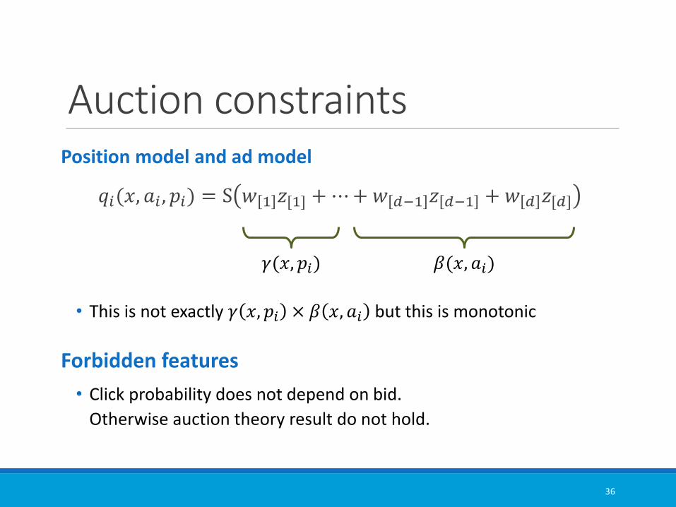
Auction constraintsPosition model and ad model

𝑞𝑖(𝑥, 𝑎𝑖 , 𝑝𝑖) = S 𝑤 1 𝑧[1] +⋯+𝑤 𝑑−1 𝑧 𝑑−1 + 𝑤 𝑑 𝑧[𝑑]

• This is not exactly 𝛾 𝑥, 𝑝𝑖 × 𝛽 𝑥, 𝑎𝑖 but this is monotonic

Forbidden features

• Click probability does not depend on bid.

Otherwise auction theory result do not hold.

𝛾(𝑥, 𝑝𝑖) 𝛽(𝑥, 𝑎𝑖)

36

Crossing and coding features• Layout• Position

𝑝𝑖

• Query ID• Query text• Date, location• Session history• …

𝑥

𝑎𝑖

• Ad ID• Ad text• Ad keywords• Advertiser ID• Bids

Crossdiscretefeatures

StatisticalModel

Crossdiscretefeatures

StatisticalModel

Codediscretefeatures

Codediscretefeatures

001000 or hashesor counts.

37

Better click prediction ≠ better systemWhich features help click prediction the most?

1. The position features (mainline vs. sidebar)

2. The context features (date, user, session history)

3. The advertiser features (some advertisers target better)

4. Finally the features crossing ad and query.

• 1 and 2 do not help picking good ads.

• 3 does not help picking ads relevant to the query.

• Only 4 makes the system markedly better.

Optimizing click prediction without understanding

the full system leads to selecting useless features.

38

Auction constraints

Using features that violate the auction theory constraints

• We know that auction theory does not model ad placement very well.

• A/B testing may show the system working better this way.

• We make the system harder to understand

Instant rewards compromise innovation speed

(see previous slide.)

• We try to do end-to-end training by hand

Worst way to do it.

(we get most of the problems and none of the benefits.)

39

4. Loops

40

Toy example

Two queriesQ1: “cheap diamonds” (50% traffic)Q2: “google” (50% traffic)

Three adsA1: “cheap jewelry”A2: “cheap automobiles”A3: “engagement rings”

More simplifications- We show only one ad per query- All bids are equal to $1.

41

Toy example

True conditional click probabilities

A1(cheap jewelry)

A2(cheap autos)

A3(engagement rings)

Q1 (cheap diamonds) 7% 2% 9%

Q2 (google) 2% 2% 2%

Step 1: pick ads randomly.

𝐶𝑇𝑅 =1

2

7 + 2 + 9

3+2 + 2 + 2

3= 4%

42

Toy exampleStep 2: estimate click probabilities

◦ Build a model based on a single Boolean feature:F : “query and ad have at least one word in common”

A1(cheap jewelry)

A2(cheap autos)



Q2 (google) 2% 2% 2%

𝑃 𝐶𝑙𝑖𝑐𝑘 𝐹 =7 + 2

2= 4.5%

𝑃 𝐶𝑙𝑖𝑐𝑘 ¬𝐹 =9 + 2 + 2 + 2

4= 3.75%

43

Toy exampleStep 3: place ads according to estimated pclick.

Q1: show A1 or A2. (predicted pclick 4.5% > 3.75%)

Q2: show A1, A2, or A3. (predicted pclick 3.75%)

A1(cheap jewelry)

A2(cheap autos)



Q2 (google) 2% 2% 2%

𝐶𝑇𝑅 =1

2

7 + 2

2+2 + 2 + 2

3= 3.25%

44

Toy exampleStep 4: re-estimate click probabilities with new data.

A1(cheap jewelry)

A2(cheap autos)



Q2 (google) 2% 2% 2%

𝑃 𝐶𝑙𝑖𝑐𝑘 𝐹 =7 + 2

2= 4.5%

𝑃 𝐶𝑙𝑖𝑐𝑘 ¬𝐹 =2 + 2 + 2

3= 2%

• We keep selecting the same inferior ads.

• Estimated click probabilities now seem more accurate.

45

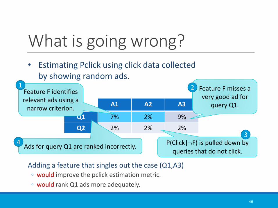
What is going wrong?

Adding a feature that singles out the case (Q1,A3)◦ would improve the pclick estimation metric.

◦ would rank Q1 ads more adequately.

A1 A2 A3

Q1 7% 2% 9%

Q2 2% 2% 2%

• Estimating Pclick using click data collected by showing random ads.

Feature F identifies relevant ads using a

narrow criterion.

1

P(Click|¬F) is pulled down by queries that do not click.

3

Ads for query Q1 are ranked incorrectly.4

Feature F misses a very good ad for

query Q1.

2

46

What is going wrong?

Adding a (Q1,A3) feature◦ would not improve the Pclick estimation on this data.

◦ would not help ranking (Q1,A3) higher.

Further feature engineering based on this data◦ would always result in eliminating more options, e.g. (Q1,A2).

◦ would never result in recovering lost options, e.g. (Q1,A3).

A1 A2 A3

Q1 7% 2% 9%

Q2 2% 2% 2%

• Re-estimating Pclick using click data collected byshowing ads suggested by the previous Pclick model.

In this data, A3 is never shown for query Q1.

𝑃(𝐶𝑙𝑖𝑐𝑘|¬𝐹) seems more accurate because we have removed the

case (Q1,A3)

47

We have created a black hole!(Q,A) can be occasionally sucked by the black hole.

◦ All kinds of events can cause ads to disappear.

◦ Sometimes, advertisers spend extra money to displace competitors.

(Q,A) can be born in the black hole.◦ Ads newly entered by advertisers

◦ Ads newly selected as eligible because of algorithmic improvements.

Exploration◦ We should sometimes show ads that we would not normally show in order

to train the click prediction model.

48

Learning feedback

User Advertiser

QueriesAds& Bids

Ads Prices

Clicks

Learning algorithm

LEARNINGFEEDBACK LOOP

Publisher

49

Programmer feedback

User Advertiser

QueriesAds& Bids

AdsPrices

Clicks Hundreds working on

the ad engine.

PROGRAMMERFEEDBACK LOOP

Publisher

50

User and advertiser feedback

Users Advertisers

QueriesAds& Bids

Ads Prices

Clicks (and consequences)

ADVERTISER FEEDBACK LOOP

USER FEEDBACK

LOOP

Publisher

51

The feedback loop problem

Shifting distributions• Data is collected when the system operates in a certain way.

The observed data follows a first distribution.

• Collected data is used to justify actions that change the operating point.Newly observed data then follows a second distribution.

• Correlations observed on data following the first distribution do not necessarily exist in the second distribution.

Often lead to vicious circles..

52

Explore/exploit trade-offExploitation• Select actions that maximize our performance metrics.

• Problem: The system will settle into a regime that might not be well described by the past data. Other regimes may be more favorable.

Exploration• Select actions that run the system in regimes that are not known,

in the hope of discovering better ways to run it.

• Problem: We may not discover anything useful.

53

Contextual banditsFramework• World select context 𝑥

• Learner chooses discrete action

𝑎 = 𝜋 𝑥 ∈ 1…𝐾

• World announces reward 𝑟(𝑥, 𝑎)

Results• Randomized data collection (i.e., exploration) enables

offline unbiased evaluation of an alternate policy 𝜋∗

by means of importance sampling.

• Solid analysis of the explore/exploit trade-off,that is, how much exploration is needed at each instant.

(Langford et al., 2008) (Li et. al., 2010, 2011)

UAI 2013 TUTORIAL 54

Structure

Actions have structure• What we learn by showing a particular ad for a particular query

tells us about showing similar ads for similar queries.

Policies have structure• One action is a set of ads displayed on a page.

But computationally feasible policies score each ad individually.

Rewards have structure• Actions are set of ads with associated click prices.

Chosen ads impact users, chosen prices impact advertisers.


The causal graph has structure

≠


5- Causation

Statistics and CausationCorrelations• Observe high correlations between events

“It is raining” and “People carry open umbrellas.”

• We can make predictions from correlations“It is raining” ⇒ “People probably carry open umbrellas.”

“People carry open umbrellas” ⇒ “It is probably raining.”

Interventions• Hypothetical

“Will it rain if we ban umbrellas?”

• Counterfactual“Would have it rained if we had banned umbrellas?”

Causality• Causal relations let us to reason on the outcome of interventions.

John Snow and the Cholera

Snake Oil ™

Snake Oil ™

60/70 [86%]10/30 [33%]

18/20 [90%]27/80 [34%]

Penicillin

PenicillinData from randomized experiment

Counterfactual estimate

• If we had given penicillin to 𝑥% of the patients,

the success rate would have been𝟏𝟗𝟒

𝟐𝟏𝟎× 𝒙 +

𝟏𝟒𝟎

𝟏𝟎𝟎𝟎× 𝟏𝟎𝟎 − 𝒙 .

• That works because the treated patients were picked randomly.

Treated Survived Success rate

w/Penicillin 210 194 92%

w/o Penicillin 1000 140 14%

Total 1210 334 27%

(not real data)

Randomized Experiments

6- Causal models

Structural equation model (SEM)

Direct causes / Known and unknown functions

Noise variables / Exogenous variables

Interventions

Interventions as algebraic manipulation of the SEM. Causal graph must remain acyclic.

* NEW Q=𝒇𝟒∗

Isolation

What to do with unknown functions?• Replace knowledge by statistics.• Statistics need repeated isolated experiments.• Isolate experiments by assuming an

unknown but invariant joint distribution for the exogenous variables.

⇒ No feedback loops (…yet…)

𝑃(𝑢, 𝑣)

Markov factorization

This is a “Bayes network” (Pearl, 1988)

a.k.a. “directed acyclic probabilistic graphical model.”

Markov interventions

Many related Bayes networks are born (Pearl, 2000)

• They are related because they share some factors.

• More complex algebraic interventions are of course possible.

*

*

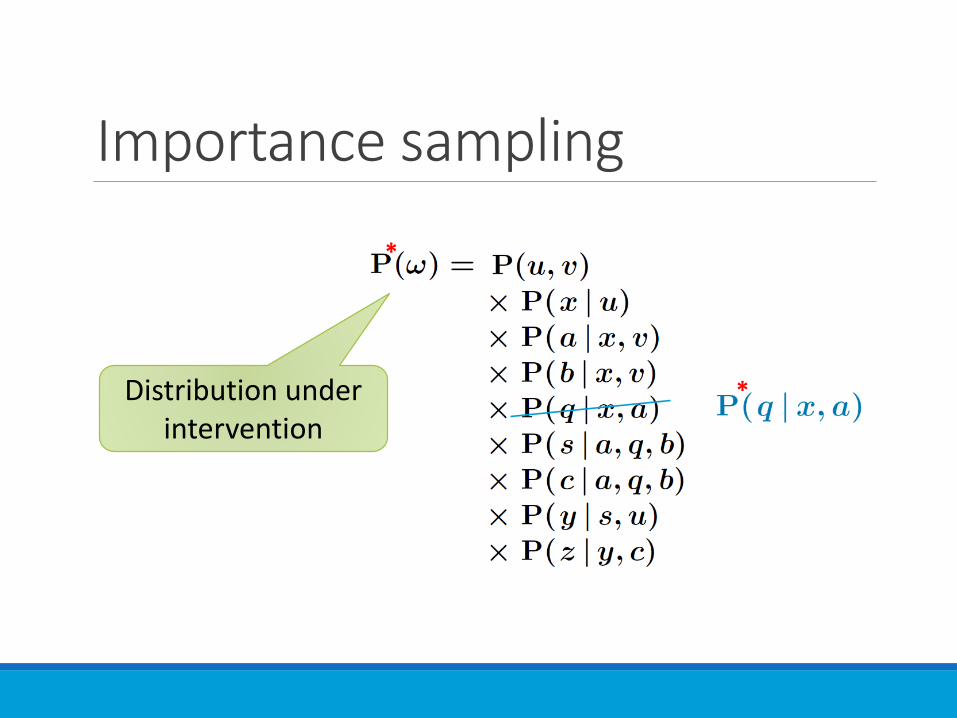
Distribution under intervention

Transfer learning on steroids

Reasoning on causal statements(laws of physics)

Experiment 1Measure 𝑔

Experiment 2Weigh rock

Experiment 3Throw rock

7-Counterfactuals

Counterfactuals

Measuring something that did not happen“How would have the system performed if, when the data was collected, we had used scoring model M’ instead of model M? ”

Learning procedure• Collect data that describes the operation of the system

during a past time period.

• Find changes that would have increased the performance of the system if they had been applied during the data collection period.

• Implement and verify…

Replaying past dataClassification example• Collect labeled data in existing setup

• Replay the past data to evaluate what the performance would have been if we had used classifier θ.

• Requires knowledge of all functions connecting the point of intervention to the point of measurement.

Replaying past dataClassification example• Collect labeled data in existing setup

• Replay the past data to evaluate what the performance would have been if we had used classifier θ.

• Requires knowledge of all functions connecting the point of intervention to the point of measurement.

𝑞

Importance sampling

*

*

Distribution under intervention

Importance sampling

Actual expectation

𝑌 = 𝜔

ℓ 𝜔 𝑃(𝜔)

Counterfactual expectation

𝑌∗ = 𝜔

ℓ 𝜔 𝑃∗(𝜔) = 𝜔

ℓ 𝜔𝑃∗(𝜔)

𝑃 𝜔𝑃(𝜔) ≈

1

𝑛

𝑖=1

𝑛𝑃∗(𝜔𝑖)

𝑃 𝜔𝑖ℓ 𝜔𝑖

Importance sampling

Principle

Reweight past examples to emulate the probability they would have had under the counterfactual distribution.

𝑤 𝜔𝑖 =𝑃∗(𝜔𝑖)

𝑃 𝜔𝑖=

𝑃∗(𝑞|𝑥, 𝑎)

𝑃(𝑞|𝑥, 𝑎)

Only requires the knowledge of the function under intervention (before and after)

Factors in P* not in P

Factors in P not in P*

Exploration

𝑃(𝜔) 𝑃∗(𝜔)

Quality of the estimation

• Large ratios undermine estimation quality.

• Confidence intervals reveal whether the data collection distribution 𝑃 𝜔 performs sufficient exploration to answer the counterfactual question of interest.

𝑃(𝜔) 𝑃∗(𝜔)

Confidence intervals

𝑌∗ = 𝜔

ℓ 𝜔 𝑤 𝜔 𝑃(𝜔) ≈1

𝑛

𝑖=1

𝑛

ℓ 𝜔𝑖 𝑤 𝜔𝑖

Using the central limit theorem?

•𝑤 𝜔𝑖 very large when 𝑃(𝜔𝑖) small.

• A few samples in poorly explored regions dominate the sum with their noisy contributions.

• Solution: ignore them.

Confidence intervals (ii)Well explored area

Ω𝑅 = 𝜔 ∶ 𝑃∗ 𝜔 < 𝑅 𝑃 𝜔

Easier estimate

𝑌∗ = Ω𝑅

ℓ 𝜔 𝑃∗ 𝜔 = 𝜔

ℓ 𝜔 𝑤 𝜔 𝑃(𝜔) ≈1

𝑛

𝑖=1

𝑛

ℓ 𝜔𝑖 𝑤 𝜔𝑖

with 𝑤 𝜔 = 𝑤(𝜔) if 𝜔 ∈ Ω𝑅

0 otherwise

This works because 0 ≤ 𝑤 𝜔 ≤ 𝑅.

Confidence intervals (iii)Bounding the bias

Assuming 0 ≤ ℓ 𝜔 ≤ 𝑀 we have

0 ≤ 𝑌∗ − 𝑌∗ ≤ Ω∖Ω𝑅

ℓ 𝜔 𝑃∗ 𝜔 ≤ 𝑀 𝑃∗ Ω ∖ Ω𝑅 = 𝑀 1 − 𝑃∗ Ω𝑅

= 𝑀 1 − 𝜔

𝑤(𝜔)𝑃(𝜔) ≈ 𝑀 1 −1

𝑛

𝑖=1

𝑛

𝑤(𝜔𝑖)

• This is easy to estimate because 𝑤(𝜔) is bounded.

• This represents the cost of insufficient exploration.

• Bonus: this remains true if 𝑃(𝜔) is zero in some places

Two-parts confidence interval

Outer confidence interval• Bounds Y∗ − Y𝑛

∗

• When this is too large, we must sample more.

Inner confidence interval

• Bounds 𝑌∗ − 𝑌∗

• When this is too large, we must explore more.

8. Example

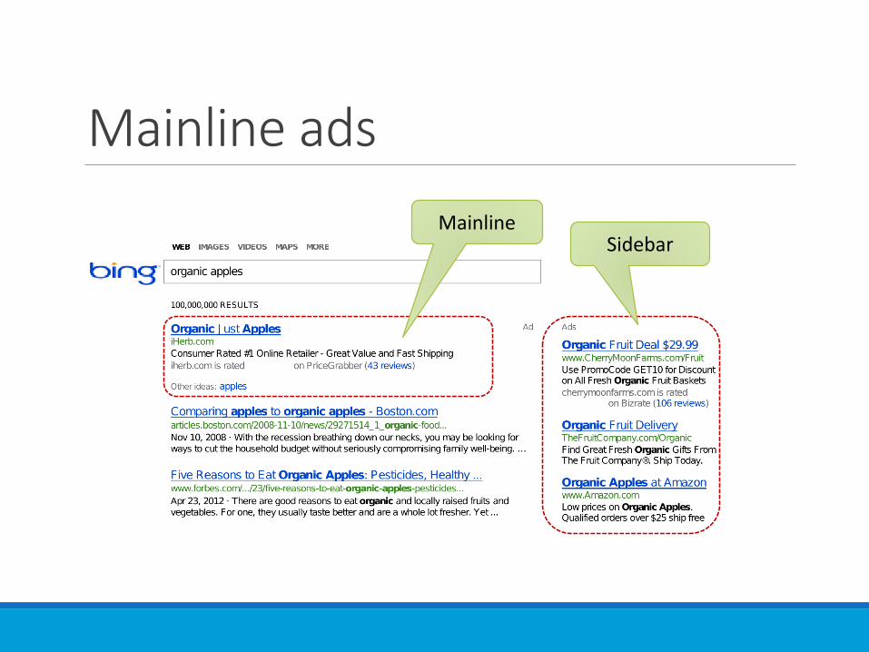
Mainline ads

MainlineSidebar

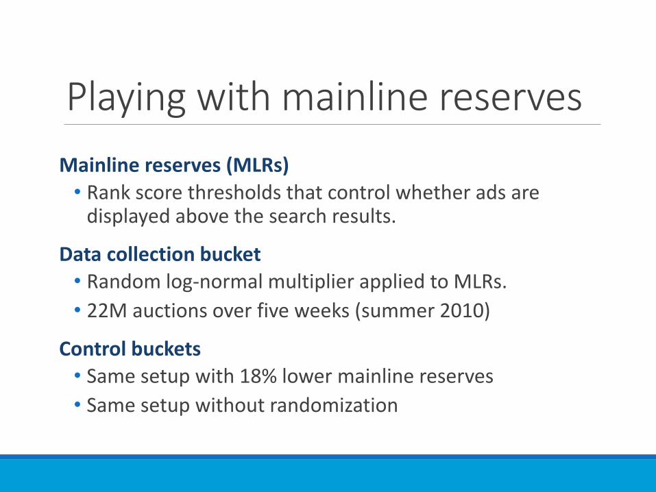
Playing with mainline reserves

Mainline reserves (MLRs)

• Rank score thresholds that control whether ads are displayed above the search results.

Data collection bucket• Random log-normal multiplier applied to MLRs.

• 22M auctions over five weeks (summer 2010)

Control buckets• Same setup with 18% lower mainline reserves

• Same setup without randomization


Inner interval

Outerinterval

Control with no randomization

Control with 18% lower MLR


This is easy to estimate


Revenue has always high

variance

More uses for the same data

Examples

Estimates for different randomization variance Good to determine how much to explore.

Query-dependent reserves Just another counterfactual distribution!

This is the big advantage

• Collect data first, choose questions later.

• Randomizing more stuff increases opportunities.

• New challenge: making sure that do not leave information on the table.

9. Structure

Shifting the reweighting point

• Users make click decisions on the basis of what they see.

• They cannot see some action variables (scores, reserves, prices, etc.)


Actual score distribution

A1 A3

A2 and many more

p=41% p=22% p=12% p=…

Counterfactual score distribution

A1A3A2

p=18% p=34% p=17% p=…

• We can estimate counterfactual click yield by reweighting the samples according to P⋄(𝑠|… ) rather than the probabilities of scores P⋄(𝑞|… ).


When can we do this?

𝑃⋄(𝜔) factorizes in the right way if and only if

1. Reweighting variables intercept every causal path connecting the point(s) of intervention to the point of measurement.

2. All functional dependencies between the point(s) of intervention and the first intercepting reweighting variable are known.

Shifting the reweighting pointExperimental validation• Mainline reserves

Score reweighting Slate reweighting

Counterfactual differencesComparing two potential interventions

Is scoring model 𝑀1 better than 𝑀2 ?

Improved confidence via variance reduction • Example: since seasonal variations affect both models nearly

identically, we can reduce the variance resulting from these variations using a predictor (a.k.a. “doubly robust”.)

Click yield if we had used model 𝑀1

Click yield if we had used model 𝑀2

Δ =

Counterfactual differences

Which scoring model works best?

• Comparing expectations under counterfactual distributions 𝑃+(𝜔) and 𝑃∗(𝜔).

𝑌+ − 𝑌∗ = 𝜔

ℓ 𝜔 − 𝜁 𝜈 Δ𝑤 𝜔 𝑃 𝜔

≈1

𝑛

𝑖=1

𝑛

ℓ 𝜔𝑖 − 𝜁(𝜈𝑖) Δ𝑤 𝜔𝑖

with Δ𝑤 𝜔 =𝑃+ 𝜔

𝑃 𝜔−

𝑃∗ 𝜔

𝑃 𝜔Variance captured by

predictor 𝜁 𝜈 is gone!

Counterfactual derivativesInfinitesimal interventions

• Related to “policy gradient” in RL.

• Can drive optimization algorithms to learn the model parameters 𝜃.

Click yield if we had used 𝑀(𝜃 + 𝑑𝜃)

Click yield if we had used model 𝑀 𝜃

𝜕𝐶𝑇𝑅

𝜕𝜃=

d𝜃

Counterfactual derivatives

Counterfactual distribution 𝑷𝜽 𝝎

𝜕𝑌𝜃

𝜕𝜃=

𝜔

ℓ 𝜔 − 𝜁 𝜈 𝑤𝜃′ 𝜔 𝑃 𝜔 ≈

1

𝑛

𝑖=1

𝑛

ℓ 𝜔𝑖 − 𝜁 𝜈𝑖 𝑤𝜃′ 𝜔𝑖

with 𝑤𝜃′ 𝜔 =

𝜕𝑤𝜃(𝜔)

𝜕𝜃= 𝑤𝜃 𝜔

𝜕 log 𝑃𝜃 𝜔

𝜕𝜃

𝑤𝜃 𝜔 can be large but there are ways…

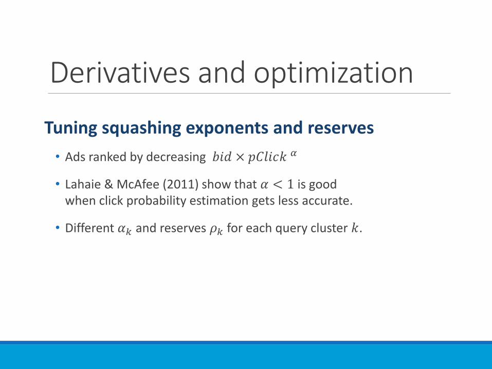
Derivatives and optimization

Tuning squashing exponents and reserves

• Ads ranked by decreasing 𝑏𝑖𝑑 × 𝑝𝐶𝑙𝑖𝑐𝑘 𝛼

• Lahaie & McAfee (2011) show that 𝛼 < 1 is good when click probability estimation gets less accurate.

• Different 𝛼𝑘 and reserves 𝜌𝑘 for each query cluster 𝑘.

Derivatives and optimization

Variation of the average number of

mainline ads.

Estimated advertiser value(arbitrary units)

Level curves for one particular query cluster

10. Equilibria

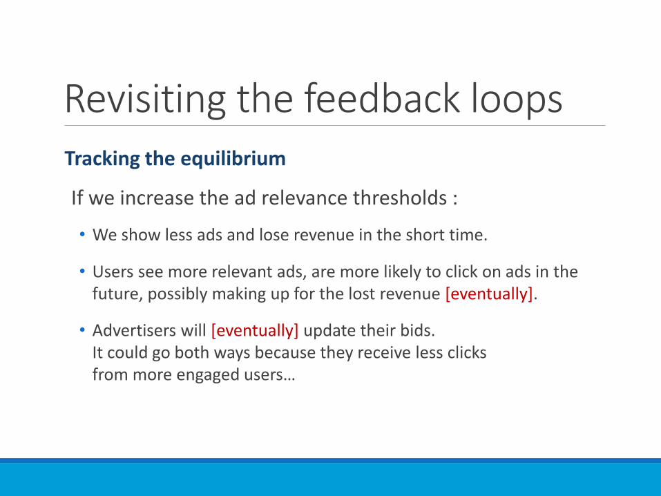
Revisiting the feedback loopsTracking the equilibrium

If we increase the ad relevance thresholds :

• We show less ads and lose revenue in the short time.

• Users see more relevant ads, are more likely to click on ads in the future, possibly making up for the lost revenue [eventually].

• Advertisers will [eventually] update their bids.It could go both ways because they receive less clicks from more engaged users…

Counterfactual equilibrium

Counterfactual question“What would have been the system performance metrics if we had applied an infinitesimal change to the parameter 𝜃 of the scoring model long enough to reach the equilibrium during the data collection period? ”

We can answer using quasi-static analysis.

(this comes from physics.)

Advertiser feedback loop

LOOP

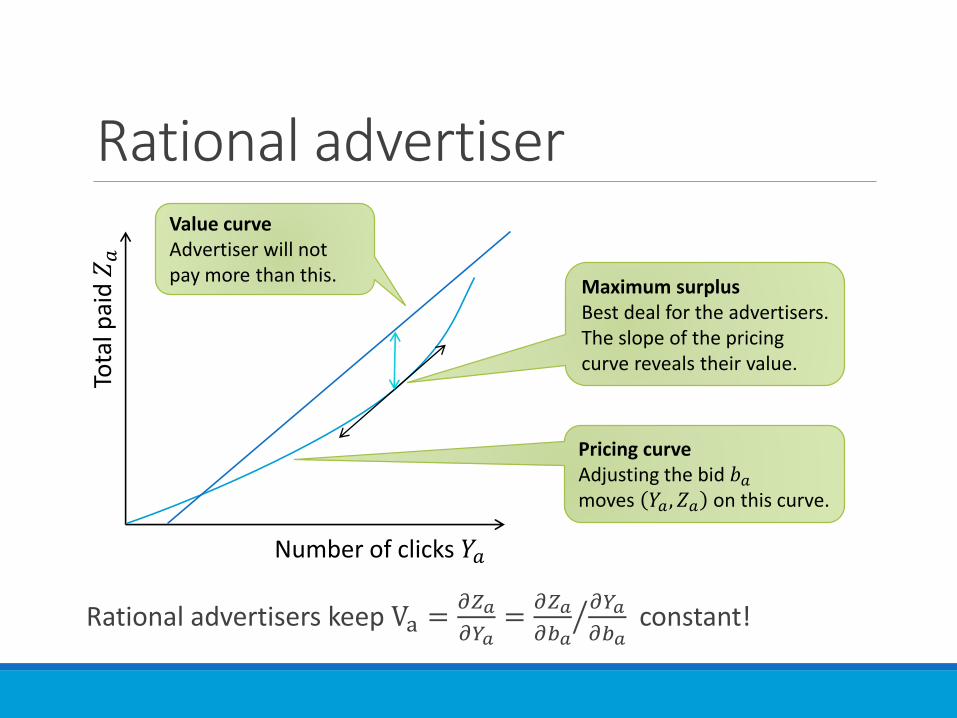
Rational advertiser

Rational advertisers keep Va =𝜕𝑍𝑎

𝜕𝑌𝑎=

𝜕𝑍𝑎

𝜕𝑏𝑎

𝜕𝑌𝑎

𝜕𝑏𝑎constant!

Number of clicks 𝑌𝑎

Tota

l pai

d 𝑍

𝑎

Pricing curveAdjusting the bid 𝑏𝑎moves 𝑌𝑎 , 𝑍𝑎 on this curve.

Value curveAdvertiser will not pay more than this.

Maximum surplusBest deal for the advertisers. The slope of the pricing curve reveals their value.

Estimating values

When the system reaches equilibrium, we can compute

Va = 𝜕𝑍𝑎𝜕𝑏𝑎

𝜕𝑌𝑎𝜕𝑏𝑎

= 𝜕𝐸𝒃,𝜃(𝑧𝑎)

𝜕𝑏𝑎

𝜕𝐸𝒃,𝜃(𝑦𝑎)

𝜕𝑏𝑎

• Complication: we cannot randomize the bids.However, since ads are ranked by bids×scores,we can interpret a random score multiplier as a random bid multiplier (need to reprice.)

Counterfactual derivatives

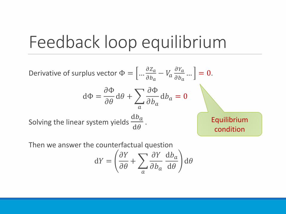
Feedback loop equilibrium

Derivative of surplus vector Φ = …𝜕𝑍𝑎

𝜕𝑏𝑎− 𝑉𝑎

𝜕𝑌𝑎

𝜕𝑏𝑎… = 0.

dΦ =𝜕Φ

𝜕𝜃d𝜃 +

𝑎

𝜕Φ

𝜕𝑏𝑎d𝑏𝑎 = 0

Solving the linear system yields d𝑏𝑎

d𝜃.

Then we answer the counterfactual question

d𝑌 =𝜕𝑌

𝜕𝜃+

𝑎

𝜕𝑌

𝜕𝑏𝑎

d𝑏𝑎d𝜃

d𝜃

Equilibrium condition

Multiple feedback loops

Same procedure:

1. Write total derivatives.

2. Solve the linear system formedby all the equilibrium conditions.

3. Substitute into the total derivativeof the counterfactual expectation of interest.

large scale machine learning in the real world · large scale machine learning in the real world...

Documents