large-scale structure in absorption: gas within and around

Mon. Not. R. Astron. Soc. 425, 245–260 (2012) doi:10.1111/j.1365-2966.2012.21448.x

Large-scale structure in absorption: gas within and around galaxy voids

Nicolas Tejos,1� Simon L. Morris,1 Neil H. M. Crighton,2 Tom Theuns,1 Gabriel Altay1

and Charles W. Finn1

1Department of Physics, Durham University, South Road, Durham DH1 3LE2Max Planck Institute for Astronomy, Konigstuhl 17, D-69117 Heidelberg, Germany

Accepted 2012 June 5. Received 2012 May 10; in original form 2012 March 22

ABSTRACTWe investigate the properties of the H I Lyα absorption systems (Lyα forest) within and aroundgalaxy voids at z � 0.1. We find a significant excess (>99 per cent confidence level, c.l.) ofLyα systems at the edges of galaxy voids with respect to a random distribution, on ∼5 h−1 Mpcscales. We find no significant difference in the number of systems inside voids with respect tothe random expectation. We report differences between both column density (NH I) and Dopplerparameter (bH I) distributions of Lyα systems found inside and at the edge of galaxy voids at the�98 and �90 per cent c.l., respectively. Low-density environments (voids) have smaller valuesfor both NH I and bH I than higher density ones (edges of voids). These trends are theoreticallyexpected and also found in Galaxies-Intergalactic Medium Interaction Calculation (GIMIC),a state-of-the-art hydrodynamical simulation. Our findings are consistent with a scenario of atleast three types of Lyα systems: (1) containing embedded galaxies and so directly correlatedwith galaxies (referred to as ‘halo-like’), (2) correlated with galaxies only because they lie inthe same overdense large-scale structure (LSS) and (3) associated with underdense LSS with avery low autocorrelation amplitude (≈random) that are not correlated with luminous galaxies.We argue that the latter arise in structures still growing linearly from the primordial densityfluctuations inside galaxy voids that have not formed galaxies because of their low densities.We estimate that these underdense LSS absorbers account for 25–30 ± 6 per cent of the currentLyα population (NH I � 1012.5 cm−2), while the other two types account for the remaining70–75 ± 12 per cent. Assuming that only NH I ≥ 1014 cm−2 systems have embedded galaxiesnearby, we have estimated the contribution of the ‘halo-like’ Lyα population to be ≈12–15 ±4 per cent and consequently ≈55–60 ± 13 per cent of the Lyα systems to be associated withthe overdense LSS.

Key words: galaxies: formation – intergalactic medium – quasars: absorption lines – large-scale structure of Universe.

1 IN T RO D U C T I O N

The intergalactic medium (IGM) hosts the main reservoirs ofbaryons at all epochs (see Prochaska & Tumlinson 2009 for areview). This is supported by both observations (e.g. Fukugita,Hogan & Peebles 1998; Fukugita & Peebles 2004; Shull, Smith &Danforth 2011) and simulations (e.g. Cen & Ostriker 1999; Theunset al. 1999; Dave et al. 2010). Efficient feedback mechanisms thatexpel material from galaxies to the IGM are required to explainthe statistical properties of the observed galaxies (e.g. Baugh et al.2005; Bower et al. 2006; Schaye et al. 2010). Given that galaxiesare formed by accreting gas from the IGM, a continuous interplay

�E-mail: [email protected]

between the IGM and galaxies is then in place. Consequently, un-derstanding the relationship between the IGM and galaxies is key tounderstanding galaxy formation and evolution. This has been recog-nized since the earliest Hubble Space Telescope (HST) spectroscopyof quasi-stellar objects (QSOs), where the association between low-z IGM absorption systems and galaxies was investigated for the firsttime (e.g. Morris et al. 1993; Spinrad et al. 1993; Morris & van denBergh 1994; Lanzetta et al. 1995; Stocke et al. 1995).

The large-scale environment in which matter resides is also im-portant, as it is predicted (e.g. Borgani et al. 2002; Padilla et al.2009) and observed (e.g. Lewis et al. 2002; Lopez et al. 2008;Padilla, Lambas & Gonzalez 2010) to have non-negligible effectson the gas and galaxy properties. Given that baryonic matter isexpected to fall into the considerably deeper gravitational poten-tials of dark matter, the IGM gas and galaxies are expected to be

C© 2012 The AuthorsMonthly Notices of the Royal Astronomical Society C© 2012 RAS

246 N. Tejos et al.

predominantly found at such locations forming the so-called ‘cos-mic web’ (Bond, Kofman & Pogosyan 1996). Identification of large-scale structures (LSS) like galaxy clusters, filaments or voids andtheir influence over the IGM and galaxies is then fundamental toa complete picture of the IGM/galaxy connection and its evolutionover cosmic time.

With the advent of big galaxy surveys such as the 2dF (Collesset al. 2001) or the Sloan Digital Sky Survey (SDSS; Abazajian et al.2009), it has been possible to directly observe the nature and extentof the distribution of stellar matter in the local Universe. Galaxiestend to lie in the filamentary structure which simulations predict;however, very little is known about the actual gas distribution at lowz. In this work, we focus on the study of H I Lyα (hereafter referredsimply as Lyα) absorption systems found within and around galaxyvoids at z � 0.1.

Galaxy voids are the best candidates to start our statistical studyof LSS in absorption. Voids account for up to 60–80 per cent ofthe volume of the universe at z = 0 (e.g. Aragon-Calvo, van deWeygaert & Jones 2010; Pan et al. 2012). Some studies have sug-gested that when a minimum density threshold is reached, voidsgrow in a spherically symmetric way (e.g. Regos & Geller 1991;van de Weygaert & van Kampen 1993). This suggests that voidshave a relatively simple geometry, which makes them compar-atively easy to define and identify from current galaxy surveys(although see Colberg et al. 2008, for a discussion on differentvoid finder algorithms). Galaxy voids are a unique environment inwhich to look for evidence of early (or even primordial) enrichmentof the IGM (e.g. Stocke et al. 2007). It is interesting that galaxyvoids are present even in the distribution of low-mass galaxies (e.g.Peebles 2001; Tikhonov & Klypin 2009) and so there must bemechanisms that prevent galaxies from forming in such low-densityenvironments.

Previous studies of Lyα absorption systems associated with voidsat low z have relied on a ‘nearest galaxy distance’ (NGD) definition(e.g. Penton, Stocke & Shull 2002; Stocke et al. 2007; Wakker &Savage 2009). In order to have a clean definition of void absorbersthe NGD must be large, leading to small samples. For instance,Penton et al. (2002) found only eight void absorbers (from a total of46 systems) defined as being located at >3 h−1

70 Mpc from the near-est ≥L∗ galaxy. Wakker & Savage (2009) found 17 void absorbers(from a total of 102) based on the same definition. Stocke et al.(2007) had to relax the previous limit to >1.4 h−1

70 Mpc in order tofind 61 void absorbers (from a total of 651 systems), although only12 were used in their study on void metallicities. Note that a lowNGD limit (of 1.4 h−1

70 Mpc) could introduce some contaminationof not-void absorbers. This is because filaments in the ‘cosmic web’are expected to be a couple of Mpc in radius (Aragon-Calvo et al.2010; Bond, Strauss & Cen 2010; Gonzalez & Padilla 2010). Con-sidering the Local Group as an example, being 1.4 h−1

70 Mpc awayfrom either the Milky Way or Andromeda cannot be consideredas being in a galaxy void. On the other hand, given that there isa population of galaxies inside voids (e.g. Rojas et al. 2005; Parket al. 2007; Kreckel et al. 2011), the NGD definition could alsomiss some ‘real’ void absorbers relatively close to bright isolatedgalaxies. In fact, Wakker & Savage (2009) found that there may beno void absorbers in their sample (based on the NGD definition) ifthe luminosity limit to the closest galaxy is reduced to 0.1L∗. Note,however, that their sample is very local (z ≤ 0.017 or �70 h−1

70 Mpcaway), and it might be biased because of the local overdensity towhich our Local Group belongs.

In this work we use a different approach to define void absorptionsystems. We based our definition on current galaxy void catalogues

(typical radius of >14 h−170 Mpc), defining void absorbers as those

located inside such galaxy voids. This leads to larger samples ofwell-identified void absorbers compared to previous studies. More-over, this approach allows us to define a sample of absorbers locatedat the very edges of voids, which can be associated with walls, fila-ments and nodes, allowing us to get some insights in the distributionof gas in the ‘cosmic web’ itself. This definition is different fromthe NGD-based ones and it focuses on the ‘large-scale’ (�10 Mpc)relationship between Lyα forest systems and galaxies. The resultsfrom this work will offer a good complement to previous studiesbased on ‘local’ scales (�2 Mpc).

Our paper is structured as follows. The catalogues of both Lyα

systems and galaxy voids that we used in this work are describedin Section 2. Definition of our LSS in absorption samples and theobservational results are presented in Section 3. We compare ourobservational results with a recent cosmological hydrodynamicalsimulation in Section 4. We discuss our findings in Section 5 andsummarize them in Section 6. A check for systematic effects andbiases that could be present in our data analysis is presented inAppendix A. All distances are in comoving coordinates assumingH0 = 100 h km s−1 Mpc−1, h = 0.71, �m = 0.27, �� = 0.73, k =0 cosmology unless otherwise stated. This cosmology was chosento match the one adopted by Pan et al. (2012) (D. Pann, privatecommunication; see Section 2.2).

2 DATA

2.1 Gas in absorption

We use QSO absorption line data from the Danforth & Shull (2008,hereafter DS08) catalogue, which is the largest high-resolution(R ≡ �λ/λ ≈ 30 000–100 000), low-z IGM sample to date.1 Briefly,the catalogue lists 651 Lyα absorption systems at zabs ≤ 0.4, withassociated metal lines [O VI, N V, C IV, C III, Si IV, Si III and Fe III;when the spectral coverage and signal-to-noise ratio (S/N) allowedtheir observation], taken from 28 active galactic nuclei (AGNs) ob-served with both the Space Telescope Imaging Spectrograph (STIS;Woodgate et al. 1998) on the HST and the Far Ultraviolet Spec-troscopic Explorer (FUSE; Moos et al. 2000). The systems arecharacterized by their rest-frame equivalent widths (Wr), or up-per limits on Wr, for each individual transition. Column densities(NH I) and Doppler parameters (bH I) were inferred using the ap-parent optical depth (AOD) method (Savage & Sembach 1991)and/or Voigt profile line fitting. In particular for the Lyα tran-sition, a curve-of-growth (COG) solution was used when otherLyman series lines were available (see also Section A2). We referthe reader to DS08 (and references therein) for further descriptionand discussion.

In order to identify absorbing gas associated with LSS[drawn from the SDSS Data Release 7 (DR7)], we use a sub-sample of the DS08 AGN sightlines that intersect the SDSSvolume (PG 0953+414, Ton 28, PG 1116+215, PG 1211+143,PG 1216+069, 3C 273, Q 1230+0115, PG 1259+593, NGC 5548,Mrk 1383 and PG 1444+407; see Table 1). Despite the fact thatPG 1216+069 spectrum has a poor quality, it is still possible to findstrong systems in it, and so we decided not to exclude it from the

1 We note that after this paper was submitted, a new preprint by Tilton et al.(2012) appeared with an updated version of the DS08 catalogue.

C© 2012 The Authors, MNRAS 425, 245–260Monthly Notices of the Royal Astronomical Society C© 2012 RAS

LSS in absorption: gas within and around voids 247

Table 1. IGM sightlines from DS08 that intersect the SDSS survey.

Sightline RA (J2000) Dec. (J2000) zAGN S/Na

PG 0953+414 09 56 52.4 +41 15 22 0.234 10 14Ton 28 10 04 02.5 +28 55 35 0.329 70 9PG 1116+215 11 19 08.6 +21 19 18 0.176 50 18PG 1211+143 12 14 17.7 +14 03 13 0.080 90 30PG 1216+069 12 19 20.9 +06 38 38 0.331 30 33C 273 12 29 06.7 +02 03 09 0.158 34 35Q 1230+0115 12 30 50.0 +01 15 23 0.117 00 12PG 1259+593 13 01 12.9 +59 02 07 0.477 80 12NGC 5548 14 17 59.5 +25 08 12 0.017 18 13Mrk 1383 14 29 06.6 +01 17 06 0.086 47 16PG 1444+407 14 46 45.9 +40 35 06 0.267 30 10

aMedian HST/STIS S/N per 2-pixel resolution element in the 1215–1340 A range (C. Danforth, private communication). The expected mini-mum equivalent width, Wmin, at a confidence level of cl corresponding to agiven S/N can be estimated from Wmin = cl ×λ

R(S/N) , where R is the spectralresolution (e.g. see DS08).

sample (this inclusion does not affect our results; see Section 3.1).2

We use the rest of the sightlines in the DS08 catalogue to derivethe general properties of the average absorber for comparison (seeSection A1).

In our analysis, we focus on statistical comparisons of the H I

properties in different LSS environments. Metal systems havesmaller redshift coverage and lower number densities than Lyα

absorbers. Consequently, we do not aim to draw statistical conclu-sions from them. We intend to pursue metallicity studies in futurework.

2.2 Galaxy voids

We use a recently released galaxy-void catalogue from SDSS DR7galaxies (Pan et al. 2012, hereafter P12), which is the largest galaxy-void sample to date. Hereafter we will use the term void to meangalaxy-void unless otherwise stated. P12 identified �1000 cosmicvoids using the VOIDFINDER algorithm described by Hoyle & Vogeley(2002), with redshifts in the range of 0.01 � z � 0.102. To summa-rize, it first uses a nearest neighbour algorithm on a volume-limitedgalaxy survey. Galaxies whose third nearest neighbour distance isgreater than 6.3 h−1 Mpc are classified as potential void galaxies,whereas the rest are classified as wall galaxies. Void regions areidentified by looking for maximal empty spheres embedded in thewall galaxy sample. These individual void spheres have radii inthe range of 10 < Rvoid � 25 h−1 Mpc, with mean radius 〈Rvoid〉 ≈13 h−1 Mpc. The minimum radius of 10 h−1 Mpc for the void sphereswas imposed. Only galaxies with spectroscopic redshifts were usedand therefore we expect the uncertainties in the void centres andradii to be small (�1 Mpc; we will discuss the effects of peculiarvelocities in Section 3.1). Independent void regions are defined bycombining all the adjacent spheres that share more than 10 per centof their volume with another. Void galaxies are defined as thosegalaxies that lie within a void region. We refer the reader to P12 forfurther description and discussion.

In our analysis, for simplicity, we use the individual spheres asseparate voids instead of using the different independent void re-

2 We note that Chen & Mulchaey (2009) have presented an Lyα absorptionsystem list along PG 1216+069 sightline at a better sensitivity than that ofDS08. In order to have an homogeneous sample, we did not include thesenew data in our analysis however.

gions. This choice has the following advantages. First, it allows usto use a perfectly spherical geometry, making it possible to char-acterize each void by just one number: its radius. Thus, we canstraightforwardly scale voids with different sizes for comparison.Secondly, this approach allows us to identify regions at the veryedges of the voids. P12 found that the number density of galaxieshas a sharp peak at a distance ≈Rvoid from the centre of the voidspheres, a clear signature that walls are well defined (at least fromthe point of view of bright galaxies at low redshifts). This is alsoconsistent with the predictions of linear gravitation theory (e.g. Icke1984; Sheth & van de Weygaert 2004) and dark matter simulations(e.g. Benson et al. 2003; Colberg et al. 2005; Ceccarelli et al. 2006;P12). Therefore, by looking for absorption systems very close tothe edge of voids, we expect to trace a different cosmic environ-ment. Thirdly, using the individual void spheres securely identifiesvoid regions. The void-edge sample on the other hand could becontaminated by void regions associated with the intersections oftwo void spheres. We checked that this is not the case though (seeSection 3.2). This contamination should only reduce any possi-ble difference between the two samples rather than enhance them.We also note that systematic uncertainties produced by assumingvoids to be perfect spheres should also act to reduce any detecteddifference.

3 DATA A NA LY SI S AND RESULTS

3.1 Number density of absorption systems around voids

We have cross-matched the IGM absorption line catalogue fromDS08 (see Section 2.1) with the void catalogue from P12 (seeSection 2.2). A total of 106 Lyα absorption systems were found inthe 11 sightlines that intersect the void sample volume (i.e. thosewith 0.01 ≤ zabs ≤ 0.102).

We first look for a possible difference in the number density ofLyα systems as a function of the distance to voids. We take twoapproaches. First, we define X as the three-dimensional distancebetween an absorption system and the closest void centre in Rvoid

units, so

X ≡ minsample

s

Rvoid, (1)

where s is the comoving distance between the centre of the closestvoid and the absorber. Thus, 0 ≤ X < 1 corresponds to absorptionsystems inside voids and X > 1 corresponds to absorption systemsoutside voids. A value of X ≈ 1 corresponds to absorption systemsaround void edges as defined by the galaxy distribution.

The second approach defines D as the three-dimensional distancebetween an absorption system and the closest void edge in comovingh−1 Mpc, so

D ≡ minsample

(s − Rvoid) [h−1 Mpc]. (2)

Negative D values correspond to absorption systems inside voids,while positive values correspond to absorbers outside voids. Valuesof D ≈ 0 h−1 Mpc are associated with absorption systems aroundvoid edges as defined by the galaxy distribution.

Distances were calculated assuming the absorption systems tohave no peculiar velocities with respect to the centre of the voids.Although this assumption might be realistic for gas inside voids, itmight not be the case for gas residing in denser environments, wheregas outflows from galaxies might dominate. However, some studieshave suggested that the bulk of Lyα forest lines have little velocityoffset with respect to galaxies (e.g. Theuns et al. 2002; Wilman


248 N. Tejos et al.

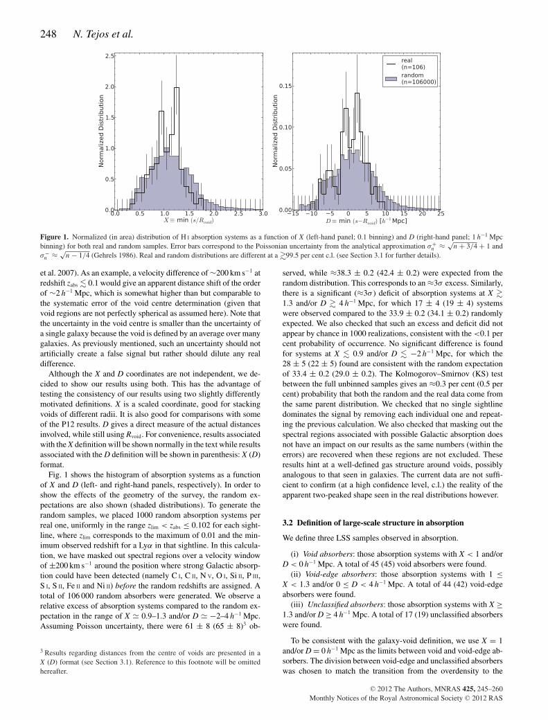
Figure 1. Normalized (in area) distribution of H I absorption systems as a function of X (left-hand panel; 0.1 binning) and D (right-hand panel; 1 h−1 Mpcbinning) for both real and random samples. Error bars correspond to the Poissonian uncertainty from the analytical approximation σ+

n ≈ √n + 3/4 + 1 and

σ−n ≈ √

n − 1/4 (Gehrels 1986). Real and random distributions are different at a �99.5 per cent c.l. (see Section 3.1 for further details).

et al. 2007). As an example, a velocity difference of ∼200 km s−1 atredshift zabs � 0.1 would give an apparent distance shift of the orderof ∼2 h−1 Mpc, which is somewhat higher than but comparable tothe systematic error of the void centre determination (given thatvoid regions are not perfectly spherical as assumed here). Note thatthe uncertainty in the void centre is smaller than the uncertainty ofa single galaxy because the void is defined by an average over manygalaxies. As previously mentioned, such an uncertainty should notartificially create a false signal but rather should dilute any realdifference.

Although the X and D coordinates are not independent, we de-cided to show our results using both. This has the advantage oftesting the consistency of our results using two slightly differentlymotivated definitions. X is a scaled coordinate, good for stackingvoids of different radii. It is also good for comparisons with someof the P12 results. D gives a direct measure of the actual distancesinvolved, while still using Rvoid. For convenience, results associatedwith the X definition will be shown normally in the text while resultsassociated with the D definition will be shown in parenthesis: X (D)format.

Fig. 1 shows the histogram of absorption systems as a functionof X and D (left- and right-hand panels, respectively). In order toshow the effects of the geometry of the survey, the random ex-pectations are also shown (shaded distributions). To generate therandom samples, we placed 1000 random absorption systems perreal one, uniformly in the range zlim < zabs ≤ 0.102 for each sight-line, where zlim corresponds to the maximum of 0.01 and the min-imum observed redshift for a Lyα in that sightline. In this calcula-tion, we have masked out spectral regions over a velocity windowof ±200 km s−1 around the position where strong Galactic absorp-tion could have been detected (namely C I, C II, N V, O I, Si II, P III,S I, S II, Fe II and Ni II) before the random redshifts are assigned. Atotal of 106 000 random absorbers were generated. We observe arelative excess of absorption systems compared to the random ex-pectation in the range of X � 0.9–1.3 and/or D � −2–4 h−1 Mpc.Assuming Poisson uncertainty, there were 61 ± 8 (65 ± 8)3 ob-

3 Results regarding distances from the centre of voids are presented in aX (D) format (see Section 3.1). Reference to this footnote will be omittedhereafter.

served, while ≈38.3 ± 0.2 (42.4 ± 0.2) were expected from therandom distribution. This corresponds to an ≈3σ excess. Similarly,there is a significant (≈3σ ) deficit of absorption systems at X �1.3 and/or D � 4 h−1 Mpc, for which 17 ± 4 (19 ± 4) systemswere observed compared to the 33.9 ± 0.2 (34.1 ± 0.2) randomlyexpected. We also checked that such an excess and deficit did notappear by chance in 1000 realizations, consistent with the <0.1 percent probability of occurrence. No significant difference is foundfor systems at X � 0.9 and/or D � −2 h−1 Mpc, for which the28 ± 5 (22 ± 5) found are consistent with the random expectationof 33.4 ± 0.2 (29.0 ± 0.2). The Kolmogorov–Smirnov (KS) testbetween the full unbinned samples gives an ≈0.3 per cent (0.5 percent) probability that both the random and the real data come fromthe same parent distribution. We checked that no single sightlinedominates the signal by removing each individual one and repeat-ing the previous calculation. We also checked that masking out thespectral regions associated with possible Galactic absorption doesnot have an impact on our results as the same numbers (within theerrors) are recovered when these regions are not excluded. Theseresults hint at a well-defined gas structure around voids, possiblyanalogous to that seen in galaxies. The current data are not suffi-cient to confirm (at a high confidence level, c.l.) the reality of theapparent two-peaked shape seen in the real distributions however.

3.2 Definition of large-scale structure in absorption

We define three LSS samples observed in absorption.

(i) Void absorbers: those absorption systems with X < 1 and/orD < 0 h−1 Mpc. A total of 45 (45) void absorbers were found.

(ii) Void-edge absorbers: those absorption systems with 1 ≤X < 1.3 and/or 0 ≤ D < 4 h−1 Mpc. A total of 44 (42) void-edgeabsorbers were found.

(iii) Unclassified absorbers: those absorption systems with X ≥1.3 and/or D ≥ 4 h−1 Mpc. A total of 17 (19) unclassified absorberswere found.

To be consistent with the galaxy-void definition, we use X = 1and/or D = 0 h−1 Mpc as the limits between void and void-edge ab-sorbers. The division between void-edge and unclassified absorberswas chosen to match the transition from the overdensity to the



Figure 2. Panels (a) and (b) show the distribution of column densities of H I as a function of X and D, respectively. Panels (c) and (d) show the distributionof Doppler parameters as a function of X and D, respectively. Our LSS samples are shown by different colours/symbols: void (black circles), void-edge (redsquares) and unclassified (blue triangles). Histograms are also shown around the main panels. Vertical red dashed lines show the limits of our LSS definitions(see Section 3.2).

underdensity of observed absorbers compared to the random ex-pectation at X > 1 and/or D > 0 h−1 Mpc (see Fig. 1).

We have assumed here that the centre of galaxy voids will roughlycorrespond to the centre of gas voids; however, that does not neces-sarily imply that gas voids and galaxy voids have the same geometry.In fact, as we do not find a significant underdensity in the numberof void absorbers with respect to the random expectation, it is notclear that such voids are actually present within the Lyα forest pop-ulation. Of course, the fact that we do not detect this underdensitydoes not imply that the gas voids are not there. A better way to lookat these definitions is by considering void absorbers as those foundin galaxy underdensities (galaxy voids) and void-edge absorbers asthose found in regions with a typical density of galaxies. We do nothave a clear picture of what the unclassified absorbers correspondto. Unclassified absorbers are those lying at the largest distancesfrom the catalogued voids, but this does not necessarily imply thatthey are associated with the highest density environments only. Infact, there could be high-density regions also located close to void-edges, at the intersection of the cosmic web filaments. Given thatvoids of radius �10 h−1 Mpc are not present in the current cata-logue, it is also likely that some of the unclassified absorbers areassociated with low-density environments. Therefore, one interpre-

tation of unclassified absorbers could be as being a mixture of allkind of environments, including voids, void-edges and high-densityregions.

We checked the robustness of these definitions by looking at thenumber of voids and void-edges which can be associated with agiven absorber. In other words, for a given absorption system, wecounted how many voids or void-edges could have been associatedwith it by taking simply X ≡ s/Rvoid or D ≡ s − Rvoid (in contrast tohaving taken the minimum values). Out of the 45 void absorbers, 41are associated with only one void and four are associated with twovoids, independently of the definition used (either X or D). Likewise,out of the 44 (42) void-edge absorbers, 31 (28) are associated withjust one void-edge, 12 (13) are associated with two void-edges and1 (1) is associated with three void-edges. This last system is locatedat X = 1.04 (D = 0.55 h−1 Mpc) and has NH I = 1014.17±0.35 cm−2

and bH I = 25+21−7 km s−1 at a redshift of zabs = 0.015 33. From these

values the system does not seem to be particularly peculiar. Findingan association with more than two void-edges is not surprising aslong as the filling factor of voids is not small.4 Void absorbers have

4 For reference, voids found by P12 have a filling factor of 62 per cent.


250 N. Tejos et al.

Table 2. General properties of our LSS samples.a

Sample log(NH I [cm−2]) bH I (km s−1)Mean Median Mean Median

Void 13.21 ± 0.67 (13.21 ± 0.67) 13.05 (13.05) 28 ± 15 (28 ± 15) 25 (25)Edge 13.50 ± 0.70 (13.52 ± 0.69) 13.38 (13.38) 33 ± 17 (34 ± 17) 28 (28)Unclassified 13.20 ± 0.45 (13.17 ± 0.48) 13.36 (13.36) 33 ± 11 (31 ± 11) 32 (31)

aResults are presented in a X (D) format (see Section 3.1).

on average 1.1 ± 0.3 voids associated with them, with a median of 1.Void-edge absorbers have on average 1.3 ± 0.5 (1.4 ± 0.5) void-edges associated with them, with a median of 1 (1). These valuesgive a median one-to-one association. Therefore, we conclude thenthat the LSS definitions used here are robust.

3.3 Properties of absorption systems in different large-scalestructure regions

Fig. 2 shows the distribution of column densities and Doppler pa-rameters as a function of both X and D. At first sight, no correlationis seen between NH I or bH I and distance to the centre of voids.Table 2 gives the mean and median values of log (NH I [cm−2]) andbH I for our void, void-edge and unclassified absorption systems.These results show consistency within 1σ between the three LSSsamples.

A closer look at the problem can be taken by investigating thepossible differences in the full NH I and bH I distributions of void,void-edge and unclassified absorbers.

3.3.1 Column density distributions

Fig. 3 shows the distribution of column density for the three differentLSS samples defined above (see Section 3.2). The top panels showthe normalized fraction of systems as a function of NH I (arbitrarybinning), whilst the bottom panels show the cumulative distribu-tions (unbinned). We see from the top panels that this distributionseems to peak systematically at higher NH I from void to void-edgeand from void-edge to unclassified absorbers. We also observe asuggestion of a relative excess of weak systems (NH I � 1013 cm−2)in voids compared to those found in void-edges. This can also beseen directly in Fig. 2 (see panels a and b). The KS test gives aprobability P

log Nvoid/edge ≈ 2 per cent (0.7 per cent) that void and void-

edge absorbers come from the same parent distribution. This impliesa >2σ difference between these samples. No significant differenceis found between voids or void-edges with unclassified absorbers,for which the KS test gives probabilities of P

log Nvoid/uncl. ≈ 74 per cent

(66 per cent) and Plog Nedge/uncl. ≈ 56 per cent (24 per cent), respectively.

These results can be understood by looking at the bottom panels ofFig. 3, as we see that the maximum difference between the void andvoid-edge absorber distributions is at NH I � 1013.8 cm−2. On theother hand, no big differences are observed at NH I � 1013.8 cm−2.In fact, by considering just the systems at NH I < 1013.8 cm−2, thesignificance of the difference between void and void-edge absorbersis increased, with P

log Nvoid/edge ≈ 0.9 per cent (0.2 per cent). Likewise,

at NH I ≥ 1013.8 cm−2, void and void-edge absorber distributionsagree at the ≈86 per cent (86 per cent) c.l. We, however, notethat there were ≤10 systems per sample for this last comparisonand therefore it is likely to be strongly affected by low numberstatistics.

Figure 3. H I column density distribution for the three different LSS samplesdefined in this work (see Section 3.2): void absorbers (solid black lines),void-edge absorbers (red dashed lines) and unclassified absorbers (bluedotted lines). The top panels show the normalized distribution using arbitrarybinning of 0.5 dex. The bottom panels show the cumulative distributionsfor the unbinned samples. The left- and right-hand panels correspond toabsorbers defined using the X and D coordinates, respectively.

We also investigated possible differences between void, void-edge and unclassified absorbers and their complements (i.e. all thesystems that were not classified as these: not-void, not-void-edge,not-unclassified). Not-voids correspond to the combination of void-edge and unclassified absorbers and so on. The KS gives probabil-ities of P

log Nvoid/not−void ≈ 4 per cent (4 per cent) and P

log Nedge/not−edge ≈

3 per cent (0.6 per cent) implying that void and void-edge ab-sorbers are somewhat inconsistent with their complements. On theother hand, the distribution of unclassified absorbers is consistentwith the distribution of their complements with a KS probabilityof P

log Nuncl./not−uncl. ≈ 64 per cent (54 per cent). These results are

summarized in Table 3.

3.3.2 Doppler parameter distributions

Fig. 4 shows the distribution of Doppler parameter for the threedifferent LSS samples defined above (see Section 3.2). The toppanels show the normalized fraction of systems as a function ofbH I (arbitrary binning), whilst the bottom panels show the cumu-lative distributions (unbinned). This figure suggests a relative ex-cess of low-bH I systems (bH I � 20 km s−1) in voids comparedto those from void-edge and unclassified samples. A relative ex-cess of unclassified absorbers compared to that of voids or void-edges at high-bH I values (bH I � 35 km s−1) is also suggested bythe figure. The KS test gives a probability P b

void/edge ≈ 8 per cent(6 per cent) that void and void-edge absorbers come from the sameparent distribution. This implies no detected difference betweenvoid and void-edge absorbers. Likewise, no significant differenceis found between voids or void-edges with unclassified absorbers,



for which the KS test gives probabilities of P bvoid/uncl. ≈ 18 per cent

(17 per cent) and P bedge/uncl. ≈ 71 per cent (75 per cent), respectively.

As before, we also investigated possible difference between LSSand their complements. In this case, void, void-edge or unclas-sified absorbers are not significantly different from their comple-ments with KS probabilities of P b

void/not−void ≈ 7 per cent (7 percent), P b

edge/not−edge ≈ 20 per cent (14 per cent) and P buncl./not−uncl. ≈

32 per cent (32 per cent). These results are also summarized inTable 3.

3.4 Check for systematic effects

Given that the differences between void and void-edge samples arestill at <3σ c.l., we have investigated possible biases or systematiceffects that could be present in our data analysis. In particular, wehave investigated (1) possible differences in our subsample withrespect to the whole DS08 sample, (2) the effect of the differentcharacterization methods used by DS08 to infer the gas propertiesand (3) whether uniformity across our redshift range is present inour observables. A complete discussion is presented in AppendixA. From that analysis, we concluded that no important biases affectour results.

4 C O M PA R I S O N W I T H SI M U L ATI O N S

In this section, we investigate whether current cosmological hy-drodynamical simulations can reproduce our observational resultspresented in Section 3. For this comparison, we use the Galaxies-Intergalactic Medium Interaction Calculation (GIMIC; Crain et al.2009).Using initial conditions drawn from the Millennium Sim-ulation (Springel et al. 2005), GIMIC follows the evolution ofbaryonic gas within five roughly spherical regions (radius between18 and 25 h−1 Mpc5) down to z = 0 at a resolution of mgas ≈107 h−1 M . The regions were chosen to have densities deviat-ing by (−2, −1, 0, +1, +2)σ from the cosmic mean at z = 1.5,where σ is the rms mass fluctuation. The +2σ region was addition-ally required to be centred on a rich cluster halo. Similarly althoughnot imposed, the −2σ region is approximately centred on a sparsevoid. The rest of the Millennium Simulation volume is resimulatedusing only the dark matter particles at much lower resolution to ac-count for the tidal forces. This approach gives GIMIC the advantageof probing a wide range of environments and cosmological featureswith a comparatively low computational expense.

GIMIC includes (i) a recipe for star formation designed to enforcea local Kennicutt–Schmidt law (Schaye & Dalla Vecchia 2008), (ii)stellar evolution and the associated delayed release of 11 chemicalelements (Wiersma et al. 2009b), (iii) the contribution of metals tothe cooling of gas in the presence of an imposed ultraviolet (UV)background (Wiersma, Schaye & Smith 2009a) and (iv) galacticwinds that pollute the IGM with metals and can quench star forma-tion in low-mass haloes (Dalla Vecchia & Schaye 2008). Note thatGIMIC does not include feedback processes associated with AGN.For further details about GIMIC we refer the reader to Crain et al.(2009).

5 Note that GIMIC adopted an H0 = 100 h km s−1Mpc−1, h = 0.73, �m =0.25, �� = 0.75, σ 8 = 0.9, k = 0 cosmology. These parameters are slightlydifferent from the ones used in P12.

4.1 Simulated H I absorbers sample

In order to obtain the properties of the simulated H I absorption sys-tems, we placed 1000 parallel sightlines within a cube of 20 h−1 Mpcon a side centred in each individual GIMIC region at z = 0 (5000sightlines in total). We have excluded the rest of the volume to avoidany possible edge effects. This roughly corresponds to 2.5 sightlinesper square h−1 Mpc. Given this density, some sightlines could betracing the same local LSS and therefore these are not fully inde-pendent. We consider this approach to offer a good compromise ofhaving a large enough number of sightlines while not oversamplingthe limited GIMIC volumes.

We used the program SPECWIZARD6 to generate synthetic normal-ized spectra associated with our sightlines using the method de-scribed by Theuns et al. (1998b). SPECWIZARD calculates the opticaldepth as a function of velocity along the line of sight, which is thenconverted to flux transmission as a function of wavelength for agiven transition. We only used H I in this calculation. The spectrawere convolved with an instrumental spread function (Gaussian)with a full width at half-maximum of 6.6 km s−1 to match the res-olution of the STIS/HST spectrograph.7 In order to mimic the con-tinuum fitting process in real spectra, we set the continuum levelof each mock noiseless spectrum at the largest flux value after theconvolution with the instrumental profile. Given that the lines aresparse at z = 0, there were almost always regions with no absorptionand this last correction was almost negligible.

We used three different S/N values in order to represent our QSOsample. Out of the total of 1000 per GIMIC regions, 727 sightlineswere modelled with S/N = 9 per pixel, 182 with S/N = 23 and91 with S/N = 2. These numbers keep the proportion between thedifferent S/N values as it is in the observed sample (see the lastcolumn in Table 1).8

We fit Voigt profiles to the synthetic spectra automatically usingVPFIT,9 following the algorithm described by Crighton et al. (2010).First, an initial guess of several absorption lines is generated ineach spectrum to minimize χ2

reduced. If the χ2reduced is greater than a

given threshold of 1.1, another absorption component is added at thepixel of largest deviation and χ2

reduced is reminimized. Absorptioncomponents are removed if both NH I < 1014.3 cm−2 and bH I <

0.4 km s−1. This iteration continues until χ2reduced ≤ 1.1. Then, the

Voigt fits are stored. We only kept absorption lines where the valuesof log NH I and bH I are at least five times their uncertainties as quotedby VPFIT.

The fraction of hydrogen in the form of H I within GIMIC isobtained from CLOUDY (Ferland et al. 1998) after assuming anionization background from Haardt & Madau (1996) that yieldsa photoionization rate of = 8.59 × 10−14 s−1. This ionizationbackground is not well constrained at z ≈ 0, so we use a post-processing correction to account for this uncertainty. In the opti-cally thin regime thin ∝ 1/τ , where τ is the optical depth (Gunn& Peterson 1965). Then, scaling the optical depth values is equiv-alent to scaling the ionization background (e.g. Theuns, Leonard& Efstathiou 1998a; Dave et al. 1999). First, we combined thefive GIMIC regions using different volume weights, namely (1/12,

6 Written by Joop Schaye, Craig M. Booth and Tom Theuns.7 Note that the majority of the Lyα used in this work were observed withSTIS/HST rather than FUSE.8 Note that we have divided the mean S/N per 2-pixel resolution element by√

2 to have an estimation per pixel.9 Written by R. F. Carswell and J. K. Webb (seehttp://www.ast.cam.ac.uk/~rfc/vpfit.html).


252 N. Tejos et al.

Table 3. KS test probabilities between different samples.a

Void/edge Void/uncl. Edge/uncl. Void/not-void Edge/not-edge Uncl./not-uncl.(per cent) (per cent) (per cent) (per cent) (per cent) (per cent)

KS-Prob(log NH I) 2 (0.7) 74 (66) 56 (24) 4 (4) 3 (0.6) 64 (54)KS-Prob(bH I) 8 (6) 18 (17) 71 (75) 7 (7) 20 (14) 32 (32)

a Results are presented in a X (D) format (see Section 3.1).

Figure 4. H I Doppler parameter distribution for the three different LSSsamples defined in this work (see Section 3.2): void absorbers (black solidlines), void-edge absorbers (red dashed lines) and unclassified absorbers(blue dotted lines). The top panels show the normalized distribution usingarbitrary binning of 5 km s−1. The bottom panels show the cumulative distri-butions for the unbinned samples. The left- and right-hand panels correspondto absorbers defined using the X and D coordinates, respectively.

1/6, 1/2, 1/6, 1/12) for the (−2, −1, 0, +1, +2)σ regions, respec-tively (see appendix 2 in Crain et al. 2009 for a justification ofthese weights). Then, we searched for a constant value to scaleall the original optical depth values such that the mean flux of thecombined sample is equal to the observed mean flux of Lyα ab-sorption at low redshift. A second possibility is to scale the opticaldepth values in order to match the redshift number density of H I

lines in some column density range, dN/dz, instead of the meanflux. Ideally, by matching one observable the second would also bematched.

Extrapolating the double power-law fit result from Kirkman et al.(2007) to z = 0 (see their equation 6), the observed mean flux is〈F〉 = 0.987 with a typical statistical uncertainty of σ 〈F〉 ∼ 0.003.In order to match this number in the simulation, a scale of 1.16is required in the original optical depth values (0.86 in ). Fromthis correction, the redshift number density of lines in the range1013.2 ≤ NH I ≤ 1014 cm−2 is found to be dN/dz ≈ 50. For reference,Lehner et al. (2007) and DS08 found dN/dz ∼ 50−90 over thesame column density range. We have repeated the experiment forconsistency, using 〈F〉 = {0.984, 0.990} which are within ±1σ 〈F〉of the extrapolated value. To match these, scales of 1.50 and 0.84are required in the original optical depth values, respectively (0.67and 1.19 in ). From those mean fluxes we found dN/dz ≈ {70,35} respectively, along the same column density range. Therefore,a value of 〈F〉 = 0.990 underpredicts the number of H I lines. On theother hand, values of 〈F〉 = 0.987 and 0.984 are in good agreementwith observations. In the following analysis, we use 〈F〉 = 0.987unless otherwise stated.

4.2 Comparison between simulated and observedH I properties

Fig. 5 shows the redshift number density of H I lines (not correctedfor incompleteness) as a function of both column density (left-handpanel) and Doppler parameter (right-hand panel). Data from the sim-ulation are shown by the black line (volume-weighted result) andeach individual GIMIC region is shown separately by the dashedlines. For comparison, data from observations are also shown. Greenopen circles correspond to the total sample from DS08 (657 sys-tems), while blue filled circles correspond to the subsample usedin this study (106 systems that intersect the SDSS volume). Thereis not perfect agreement between simulated and real data. We seean excess (lack) of systems with NH I � 1013.5 cm−2 (�1014 cm−2)in the simulation compared to observations while Doppler param-eters are in closer agreement, although there is still a difference atlow bH I.

Assuming that the column density distribution can be modelledas a power law, the position of the turnover at the low NH I endgives us an estimation of the completeness level of detection in thesample. As the turnover appears to be around NH I ≈ 1013 cm−2 inboth simulated and real data (by design), we do not, in principle,attribute the discrepancy in the column density distributions to awrong choice of the simulated S/N. Raising the mean flux to agreater value than 〈F〉 = 0.987 (less absorption) does not help as thedN/dz in the range 1013.2 ≤ NH I ≤ 1014 cm−2 will then be smallerthan the observational result (see Section 4.1). We attempted to get abetter match by using a mean flux of 〈F〉 = 0.984 (more absorption),motivated to produce a better agreement at higher column densities.In order to agree at low column densities, we had to degrade thesample S/N to be composed of ∼400, ∼100 and ∼500 sightlines atS/N values of 9, 23 and 2, respectively. It is implausible that half ofthe observed redshift path has such a poor quality.

Another possibility to explain the discrepancy could be the factthat weak systems in observations were preferentially character-ized with the AOD method, whereas here we have only used Voigtprofile fitting. In order to test this hypothesis, we have mergedclosely separated systems (within 150 km s−1) whose summed col-umn density is less than 1013.5 cm−2. Using these constraints, 43 outof 4179 systems were merged (≈1 per cent). Such a small fractiondoes not have an appreciable effect on the discrepancy. As an ex-treme case, we have repeated the experiment merging all systemswithin 300 km s−1 independently of their column densities. Fromthis, 555 out of 4179 systems were merged (≈13 per cent) but stillit was not enough to fully correct the discrepancy. Given that thediscrepancy is not explained by a systematic effect from differ-ent line characterization methods, we chose to keep our originalsimulated sample in the following analysis without merging anysystems.

There is a reported systematic effect by which column densitiesinferred from a single Lyα line are typically (with large scatter)underestimated with respect to the COG solution. Similarly bH I aretypically overestimated (Shull et al. 2000; Danforth et al. 2006;



Figure 5. Redshift number density of H I lines as a function of both column density (left-hand panel) and Doppler parameter (right-hand panel) using arbitrarybinning of � log NH I = 0.2 dex and �bH I = 5 km s−1, respectively. Both results have not been corrected for incompleteness. Green open circles correspondto real data from the total sample of DS08 (657 systems), while blue filled circles (slightly offset in the x-axes for clarity) correspond to the subsample used inthis study (106 systems). The black line corresponds to the volume-weighted result from the combination of the five GIMIC regions where the shaded regioncorresponds to the ±1σ uncertainty. Dashed lines show the results from each individual GIMIC region. Error bars correspond to the Poissonian uncertaintyfrom the analytical approximation σ+

n ≈ √n + 3/4 + 1 and σ−

n ≈ √n − 1/4 (Gehrels 1986).

see also Section A2 for discussion on how this may affect ourobservational results). This effect is only appreciable for NH I �1014 cm−2 and is bigger for saturated lines. Given that our simulatedsample was constructed to reproduce the observed sample, thiseffect could be present. If so, it would, in principle, help to reducethe discrepancy at the high column density end. From fig. 3 ofDanforth et al. (2006), we have inferred a correction for systemswith NH I ≥ 1013.5 cm−2 of

log N corrH I = log Nobs

H I − 8.37

1 − 0.62, (3)

where N corrH I and Nobs

H I are the corrected and observed NH I values,respectively. From this correction, we found an increase in thenumber of systems at NH I � 1014.5 cm−2 up to values consistentwith observations. This, however, does not help with the discrepancyat lower column densities.

At this point, it is difficult to reconcile the simulation result withthe real data using only a single effect. We note that the discrepancyis a factor of ∼2 only, so it could be in principle explained througha combination of several observational effects. Also note that thenumber of observed lines at higher column densities is still small andit could be affected by low number statistics. The lack of systemswith very low NH I and bH I values can be explained by our selectionof the highest S/N value of 23, while in real data there could beregions with higher values. It is not the aim of this section to havea perfect match between simulations and observations, but ratherexamine the qualitative differences between simulated regions ofdifferent densities. Thus, hereafter, we will use the results from thesimulation in its original form (as shown in Fig. 5), i.e. without anyof the aforementioned corrections.

4.3 Simulated H I absorbers’ properties in differentLSS regions

Given that GIMIC does not provide enough volume to perform acompletely analogous search for voids (each region is ∼20 h−1 Mpc

of radius), we use them only as crude guides to compare our resultswith. We could consider the −2σ region as representative of voidregions as it is actually centred in one. Naively, we could considerthe 0σ regions as representative of void-edge regions, as it is therewhere the mean cosmological density is reached. A direct associa-tion for the +1σ and +2σ is not so simple though, as they would beassociated with some portions of the void-edge regions too. It seemsmore reasonable to use the GIMIC spheres as representative of dif-ferent density environments then, where −2σ /+2σ correspond toextremely underdense/overdense regions and so on. For reference,the whole (−2, −1, 0, +1, +2)σ GIMIC regions correspond todensities of ρ/〈ρ〉 ≈ (0.4, 0.6, 0.9, 1.2, 1.8)10 at z = 0, respectively,where 〈ρ〉 is the mean density of the Universe (see fig. A1 fromCrain et al. 2009).

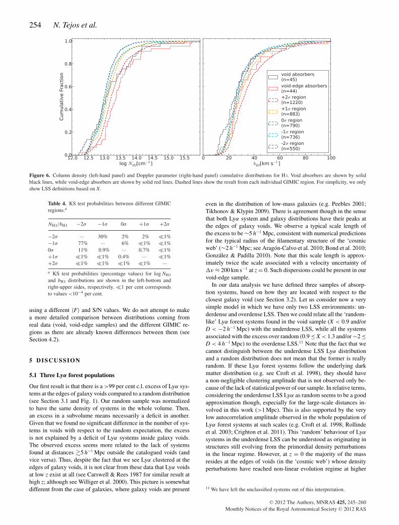
Fig. 6 shows the cumulative distributions of NH I (left-hand panel)and bH I (right-hand panel). Results from each of the individualGIMIC region are shown by dashed lines. Void and void-edge ab-sorbers are shown by solid black and red lines, respectively. Forsimplicity, we show only LSS definition based on X. Cumulativedistributions between real and simulated data do not agree perfectly.However, in both real and simulated data, there is an offset betweencolumn densities and Doppler parameters found in different envi-ronments. Low-density environments have smaller values for bothNH I and bH I than higher density ones (and vice versa). This trendstill holds when using an S/N = 23 per pixel for the 5000 sightlines.

The KS test gives a significant difference between the +2σ , +1σ

and +0σ regions, and any other GIMIC region at the �99 percent, �99 per cent and �95 per cent c.l., respectively, in both NH I

and bH I distributions. The KS test gives no significant differencebetween the −2σ and −1σ regions in both NH I and bH I distri-butions (see Table 4). These results do not change significantlywhen correcting GIMIC to match the observed NH I distribution

10 Given that we are using cubic subvolumes centred in these spheres, thesecubes should have higher density differences between them.


254 N. Tejos et al.

Figure 6. Column density (left-hand panel) and Doppler parameter (right-hand panel) cumulative distributions for H I. Void absorbers are shown by solidblack lines, while void-edge absorbers are shown by solid red lines. Dashed lines show the result from each individual GIMIC region. For simplicity, we onlyshow LSS definitions based on X.

Table 4. KS test probabilities between different GIMICregions.a

NH I/bH I −2σ −1σ 0σ +1σ +2σ

−2σ ··· 30% 2% 2% �1%−1σ 77% ··· 6% �1% �1%0σ 11% 0.9% ··· 0.7% �1%+1σ �1% �1% 0.4% ··· �1%+2σ �1% �1% �1% �1% ···a KS test probabilities (percentage values) for log NH I

and bH I distributions are shown in the left-bottom andright-upper sides, respectively. �1 per cent correspondsto values <10−4 per cent.

using a different 〈F〉 and S/N values. We do not attempt to makea more detailed comparison between distributions coming fromreal data (void, void-edge samples) and the different GIMIC re-gions as there are already known differences between them (seeSection 4.2).

5 D ISCUSSION

5.1 Three Lyα forest populations

Our first result is that there is a >99 per cent c.l. excess of Lyα sys-tems at the edges of galaxy voids compared to a random distribution(see Section 3.1 and Fig. 1). Our random sample was normalizedto have the same density of systems in the whole volume. Then,an excess in a subvolume means necessarily a deficit in another.Given that we found no significant difference in the number of sys-tems in voids with respect to the random expectation, the excessis not explained by a deficit of Lyα systems inside galaxy voids.The observed excess seems more related to the lack of systemsfound at distances �5 h−1 Mpc outside the catalogued voids (andvice versa). Thus, despite the fact that we see Lyα clustered at theedges of galaxy voids, it is not clear from these data that Lyα voidsat low z exist at all (see Carswell & Rees 1987 for similar result athigh z; although see Williger et al. 2000). This picture is somewhatdifferent from the case of galaxies, where galaxy voids are present

even in the distribution of low-mass galaxies (e.g. Peebles 2001;Tikhonov & Klypin 2009). There is agreement though in the sensethat both Lyα system and galaxy distributions have their peaks atthe edges of galaxy voids. We observe a typical scale length ofthe excess to be ∼5 h−1 Mpc, consistent with numerical predictionsfor the typical radius of the filamentary structure of the ‘cosmicweb’ (∼2 h−1 Mpc; see Aragon-Calvo et al. 2010; Bond et al. 2010;Gonzalez & Padilla 2010). Note that this scale length is approx-imately twice the scale associated with a velocity uncertainty of�v ≈ 200 km s−1 at z = 0. Such dispersions could be present in ourvoid-edge sample.

In our data analysis we have defined three samples of absorp-tion systems, based on how they are located with respect to theclosest galaxy void (see Section 3.2). Let us consider now a verysimple model in which we have only two LSS environments: un-derdense and overdense LSS. Then we could relate all the ‘random-like’ Lyα forest systems found in the void sample (X < 0.9 and/orD < −2 h−1 Mpc) with the underdense LSS, while all the systemsassociated with the excess over random (0.9 ≤ X < 1.3 and/or −2 ≤D < 4 h−1 Mpc) to the overdense LSS.11 Note that the fact that wecannot distinguish between the underdense LSS Lyα distributionand a random distribution does not mean that the former is reallyrandom. If these Lyα forest systems follow the underlying darkmatter distribution (e.g. see Croft et al. 1998), they should havea non-negligible clustering amplitude that is not observed only be-cause of the lack of statistical power of our sample. In relative terms,considering the underdense LSS Lyα as random seems to be a goodapproximation though, especially for the large-scale distances in-volved in this work (>1 Mpc). This is also supported by the verylow autocorrelation amplitude observed in the whole population ofLyα forest systems at such scales (e.g. Croft et al. 1998; Rollindeet al. 2003; Crighton et al. 2011). This ‘random’ behaviour of Lyα

systems in the underdense LSS can be understood as originating instructures still evolving from the primordial density perturbationsin the linear regime. However, at z = 0 the majority of the massresides at the edges of voids (in the ‘cosmic web’) whose densityperturbations have reached non-linear evolution regime at higher

11 We have left the unclassified systems out of this interpretation.



redshifts. For reference, we expect the underdense and overdenseLSS to have typical δ � 0 and δ � 0 respectively, where δ is thedensity contrast defined as

δ ≡ ρ − 〈ρ〉〈ρ〉 , (4)

where ρ is the density and 〈ρ〉 is the mean density of the Universe.Note, however, that these LSS environments are not defined by aparticular density but rather by a topology (voids, walls, filaments).

Theoretical arguments point out that the observed column densityof neutral hydrogen at a fixed z is

NH I ∝ ρ1.5H T −0.26 −1 f 0.5

g , (5)

where ρH is the density of hydrogen, T is the temperature of the gas, is the hydrogen photoionization rate and fg is the fraction of massin gas (Schaye 2001). In the diffuse IGM it has been predicted thatT ∝ ρα

H, where α ≈ 0.59 (Hui & Gnedin 1997). This implies that fora fixed , the main dependence of NH I is due to ρH as NH I ∝ ρ1.4

H .Then, despite the extremely low densities inside galaxy voids wecan still observe Lyα systems, although only the ones correspondingto the densest structures.

Let us consider the predicted ratio between NH I observed insidevoids and at the edges of voids as

NvoidH I

NedgeH I

≈(

ρvoidH

ρedgeH

)1.4 (void

edge

)−1(

f voidg

fedgeg

)0.5

. (6)

Given that the time-scale for photons to travel along ∼10–20 h−1 Mpc is �1 Gyr, we can consider void ≈ edge. Even ifwe assume that the gas inside voids has not formed galaxies,f void

g � f edgeg , because fg is dominated by the dark matter. This im-

plies that a given observed NH I inside and at the edge of galaxy voidswill correspond to similar densities of hydrogen (ρvoid

H ≈ ρedgeH ).

This is important because it means that the Lyα forest in the un-derdense LSS is not different from the overdense LSS one, andtwo systems with equal NH I are comparable, independently of itslarge-scale environment.

If there were no galaxies, this simple model may suffice to explainthe differences in the observed Lyα population. The fact that someof the Lyα systems are directly associated with galaxies cannot beneglected though. There is strong evidence from observations (e.g.Lanzetta et al. 1995; Chen et al. 1998; Morris & Jannuzi 2006;Stocke et al. 2006; Chen & Mulchaey 2009; Crighton et al. 2011;Prochaska et al. 2011; Rakic et al. 2012; Rudie et al. 2012) andsimulations (e.g. Fumagalli et al. 2011; Stinson et al. 2011) thatNH I � 1015 cm−2 systems are preferentially found within a coupleof hundred kpc of galaxies. Probably an appropriate interpreta-tion of such a result is that galaxies are always found in ‘local’(�100 h−1 kpc) high density regions. Then, a plausible scenariowould require at least three types of Lyα forest systems: (1) con-taining embedded galaxies, (2) associated with overdense LSS butwith no close galaxy and (3) associated with underdense LSS butwith no close galaxy. For convenience, we will refer to the first typeas ‘halo-like’, although with the caution that these systems may notbe gravitationally bound with the galaxy.

Given that there are galaxies inside galaxy voids, the ‘halo-like’Lyα systems will be present in both low- and high-density LSSenvironments (galaxies are a ‘local’ phenomenon). The contributionof the ‘halo-like’ in galaxy voids could be considered small though.Assuming this contribution to be negligible, we can estimate thefraction of Lyα systems in the underdense LSS as ≈25−30 ± 6 per

cent.12 Likewise, ≈70–75 ± 12 per cent of the Lyα forest populationis due to a combination of systems associated with galaxies and withthe overdense LSS. We could estimate the contribution of ‘halo-like’absorbers by directly looking for and counting galaxies relativelyclose to the absorption systems. A rough estimation can be doneby assuming that galaxy haloes will have only NH I ≥ 1014 cm−2

systems, leading to a contribution of ≈12–15 ± 4 per cent13 in oursample.

In summary, our results require at least three types of Lyα systemsto explain the observed Lyα forest population at low-z (NH I �1012.5 cm−2).

(i) Halo-like: Lyα with embedded nearby galaxies(�100 h−1 kpc) and so directly correlated with galaxies (≈12–15 ±4 per cent).

(ii) Overdense LSS: Lyα associated with the overdense LSS thatare correlated with galaxies only because both populations lie in thesame LSS regions (≈50–55 ± 13 per cent).

(iii) Underdense LSS: Lyα associated with the underdense LSSwith very low autocorrelation amplitude that are not correlated withgalaxies (≈25–30 ± 6 per cent).

The relative contribution of these different Lyα populations is afunction of the lower NH I limit. Low NH I systems dominate theLyα column density distribution. Then, given that underdense LSSLyα systems tend to be of lower column density than the other twotypes, we expect the contribution of ‘random-like’ Lyα to increase(decrease) while observing at lower (higher) NH I limits. Note thatthere are not sharp NH I limits to differentiate between our threepopulations (see Fig. 2). The ‘halo-like’ is defined by being close togalaxies, while the ‘LSS-like’ ones are defined in terms of an LSStopology (voids, wall, filaments).

Motivated by a recently published study on the Lyα/galaxy as-sociation by Prochaska et al. (2011), we can set a conservative up-per limit to the ‘halo-like’ contribution. These authors have foundthat nearly all their observed L ≥ 0.01L∗ galaxies (33/37) haveNH I ≥ 1013.5 cm−2 absorption at impact parameters <300 h−1

72 kpc.If we invert the reasoning and assume an extreme (likely unrealistic)scenario where all the NH I ≥ 1013.5 cm−2 are directly associatedwith galaxies, then the ‘halo-like’ contribution will have an up-per limit of <33 ± 7 per cent.14 Consequently, the contributionof the overdense LSS to the Lyα population will be >37–42 ±14 per cent. Still, note that we have found several systems with1013.5 � NH I � 1014.5 cm−2 inside galaxy voids for which a directassociation with galaxies is dubious (see Fig. 2). Also note thatonly ∼10 per cent (∼0 per cent) of the Lyα systems in the rangeof 1013.5 < NH I < 1014.5 cm−2 may be associated with a galaxyat impact parameters <300 kpc (<100 kpc) in the Prochaska et al.(2011) sample (see their fig. 4).

Our findings are consistent with previous studies pointing out anon-negligible contribution of ‘random’ Lyα systems (at a similarNH I limit) of ≈20–30 per cent (Mo & Morris 1994; Stocke et al.1995; Penton et al. 2002). These authors estimated that ≈70–80 percent of the Lyα population is associated with either LSS (galaxy

12 These numbers come from 28 ± 5 (22 ± 5) and 61 ± 8 (65 ± 8) systemsfound at X < 0.9 (D < −2 h−1 Mpc) and at 0.9 ≤ X < 1.3 (−2 ≤ D <

4 h−1 Mpc), respectively (see Section 3.1).13 From either 13/89 (excluding the unclassified sample) or 13/106 (includ-ing the unclassified sample). We have assumed Poisson uncertainty.14 From either 29/89 (excluding the unclassified sample) or 35/106 systemsin our sample (including the unclassified sample). We have assumed Poissonuncertainty.


256 N. Tejos et al.

filaments) or galaxies. Note that Mo & Morris (1994) put an upperlimit of ≈20 per cent being directly associated with galaxies, whichis also consistent with our estimation. Our result is also in accor-dance with the previous estimation that 22 ± 8 per cent (Pentonet al. 2002; based on eight systems) and 17 ± 4 per cent (Wakker &Savage 2009; based on 17 systems) of the Lyα systems lie in voids(defined as locations at >3 h−1

70 Mpc from the closest >L∗ galaxy).This is in contrast with early models that associated all Lyα systemswith galaxies (e.g. Lanzetta et al. 1995; Chen et al. 1998).

Although there is general agreement with recently proposed mod-els to explain the origin of the low-z Lyα forest (e.g. Wakker &Savage 2009; Prochaska et al. 2011), we emphasize that our inter-pretation is qualitatively different and adds an important componentto the picture: the presence of the underdense LSS (‘random-like’)systems. For instance, assuming infinite filaments of typical widthsof ≈400 h−1

72 kpc around galaxies, Prochaska et al. (2011) arguedthat all Lyα systems at low z belong either to the circumgalac-tic medium (CGM;15 which includes our ‘galaxy halo’ definition)or the filamentary structure in which galaxies reside (equivalentto our overdense LSS definition). Our findings are not fully con-sistent with this hypothesis, as neither the ‘CGM model’ nor the‘galaxy filament model’ seem likely to explain the majority of ourunderdense LSS absorbers at NH I � 1013.5 cm−2. To do so therewould need to be a whole population of unobserved galaxies (dwarfspheroidals?) inside galaxy voids with an autocorrelation amplitudeas low as the ‘random-like’ Lyα one. As discussed by Tikhonov& Klypin (2009), very low surface brightness dwarf spheroidalscould be a more likely explanation than dwarf irregulars becausethe latter should have been observed with higher incidences in re-cent H I emission blind surveys inside galaxy voids (e.g. Doyleet al. 2005). On the other hand, the formation of dwarf spheroidalsinside galaxy voids is difficult to be explained from the currentgalaxy formation paradigm (see Tikhonov & Klypin 2009 for fur-ther discussion). As mentioned, it seems more natural to relate themajority of the underdense LSS absorbers with the peaks of ex-tremely low-density structures inside galaxy voids, still evolvinglinearly from the primordial density perturbations that have not yetformed galaxies because of their low densities. Our interpretationcan be tested by searching for galaxies close to our lowest NH I

void absorbers (see Fig. 2). Another prediction of our interpreta-tion is that the vast majority of NH I � 1013 cm−2 systems shouldreside inside galaxy voids. If the QSO sightlines used here wereobserved at higher sensitivities, weak Lyα systems should prefer-entially appear at X < 1 (D < 0 h−1 Mpc). Therefore, we shouldexpect to have an anticorrelation between NH I � 1013 cm−2 andgalaxies.

5.2 NH I and bH I distributions

Our second result is that there is a systematic difference (�98 percent c.l.) between the column density distributions of Lyα systemsfound within, and those found at the edge of, galaxy voids. Voidabsorbers have more low column density systems than the void-edge sample (see Fig. 3). A similar trend is found in GIMIC, where

15 According to the Prochaska et al. (2011) definition ‘the CGM correspondsto highly ionized medium around galaxies at distances greater than thevirial radius but smaller than ∼300 kpc that need not be causally connected(associated, gravitationally bound) with these galaxies’. We do not see a clearadvantage of adopting this terminology and so we use ‘IGM’ instead to referto the same medium. We only make a distinction between LSS (voids, walls,filaments) and the ones with embedded nearby galaxies (�100 h−1 kpc).

low-density environments present smaller NH I values than higherdensity ones (see Fig. 6, left-hand panel). This can be explained bythe fact that baryonic matter follows the underlying dark matter dis-tribution. Then, the highest density environments should be locatedat the edges of voids (in the intersection of walls and filaments),consequently producing higher column density absorption than ingalaxy voids (e.g. see Schaye 2001).

Also, by construction, there is a higher chance to find galaxies atthe edges rather than inside galaxy voids. Assuming that some ofthe Lyα forest systems are associated with galaxy haloes (see Sec-tion 5.1 for further discussion), this population should be presentmainly in our void-edge sample. As galaxy haloes correspond tolocal density peaks, we should also expect on average higher col-umn density systems in this population. Given that galaxies mayaffect the properties of the surrounding gas, there could be pro-cesses that only affect Lyα systems close to galaxies. For instance,the distribution of Lyα systems around galaxy voids seems to showa two-peaked shape (see Fig. 1). We speculate that this could be asignature of neutral hydrogen being ionized by the UV backgroundproduced by galaxies (see also Adelberger et al. 2003), mostly af-fecting NH I � 1013 cm−2 inside the filamentary structure of the‘cosmic web’. Another explanation could be that in the inner partsof the filamentary structure, Lyα systems get shock heated by thelarge gravitational potentials, raising their temperature and ioniza-tion state (e.g. Cen & Ostriker 1999). A third possibility is that itcould be a signature of bulk outflows as the shift between peaksis consistent with a �v ≈ 200–300 km s−1. On the other hand, thetwo peaks could have distinct origins as the first one may be relatedto an excess of NH I � 1013 cm−2 systems, probably associatedwith the overdense LSS in which galaxies reside, while the sec-ond one may be related to an excess of NH I � 1014 cm−2 systems,more likely associated with systems having embedded galaxies. Asmentioned, we cannot prove the reality of this two-peaked signa-ture at a high confidence level from the current sample and so weleave the confirmation or disproof of these hypotheses to futurestudies.

The GIMIC data analysis shows a clear differentiation of bH I

distributions in different density environments (see Fig. 6, right-hand panel). Low-density environments have smaller bH I valuesthan higher density ones. We see a similar trend in the real databetween our void and void-edge absorber samples, although only ata �90 per cent c.l. (i.e. not very significant; see Fig. 4). The mainmechanisms that contribute to the observed line broadening are tem-perature, local turbulence and bulk motions of the gas (excludingsystematic effects from the line fitting process or degeneracy withNH I for saturated lines). Naturally, in high-density environments,we would expect to have greater contributions from both local tur-bulence and bulk motions compared to low-density ones. The gastemperature is also expected to increase from low-density environ-ments to high-density ones. As previously mentioned, theoreticalarguments predict that the majority of the diffuse IGM will havetemperatures related to the density by T ∝ ρα with α > 0 (Hui& Gnedin 1997; Theuns et al. 1998b; Schaye et al. 1999). Thisis also seen in density–temperature diagrams drawn from currenthydrodynamical cosmological simulations (e.g. Dave et al. 2010;Tepper-Garcıa et al. 2012). Therefore, our findings are consistentwith current expectations.

5.3 Future work

The high sensitivity of the recently installed Cosmic Origins Spec-trograph (COS/HST; Green et al. 2012) in the UV (especially the



far-UV) will allow us to improve the NH I completeness limit com-pared with current surveys. This will considerably increase the num-ber of observed Lyα absorption systems at low-z. In the short term,there are several new QSO sightlines scheduled for observations (oralready observed) with COS/HST that intersect the SDSS volume.Combining these with current and future galaxy void catalogues, weexpect to increase the statistical significance of the results presentedin this work. COS/HST will also allow observations of considerablymore metal lines (especially O VI) than current IGM surveys. Again,in combination with LSS surveys, this will be very useful for stud-ies on metal enrichment in different environments. For instance, wehave identified eight systems with observed O VI absorption fromSTIS/HST in our sample. Three of these lie inside voids at X ≈ {0.6,0.7, 0.9} (D ≈ {−5.4, −4.6, −1.6} h−1 Mpc), respectively. The firsttwo systems that lie inside voids correspond to the highest NH I val-ues (NH I > 1014.5 cm−2; see Fig. 2). We have performed a searchin the SDSS DR8 for galaxies in a cylinder of radius 1 h−1

71 Mpcand within ±200 km s−1 around these two absorbers (both systemsbelong to the same sightline and are at a similar redshift; one ofthem shows C IV absorption also). We found nine galaxies withthese constraints, hinting on a possible association of these sys-tems with a void galaxy. The one at the very edge of the voidlimit has NH I = 1013.14±0.07 cm−2 and NO VI = 1013.69±0.18 cm−2,and it could in principle be associated with the overdense LSS.The other five O VI absorbers lie in our void-edge sample and haveNH I > 1013.5 cm−2, so they are likely to be associated with galax-ies. None of the observed O VI lie in our unclassified sample. Thecurrent sample of O VI systems is very small, and so we do not aimto draw statistical conclusions from them. However, these systemsindividually offer interesting cases worth further investigation. Weintend to perform a careful search for galaxies that could be asso-ciated with each of the Lyα absorbers presented in our sample infuture work. In the longer term, it will be possible to extend similaranalysis to well-defined galaxy filaments and clusters when the newgeneration of galaxy surveys are released.

A scenario with three different types of Lyα forest systems, asproposed here, can help to interpret recent measurements of thecross-correlation between Lyα and galaxies (Chen et al. 2005; Ryan-Weber 2006; Wilman et al. 2007; Chen & Mulchaey 2009; Shoneet al. 2010; Rudie et al. 2012). These studies come mainly frompencil beam galaxy surveys around QSO sightlines where iden-tifying LSS such as voids or filaments is more challenging. Asmentioned, different Lyα systems are not separated by well-definedNH I limits and so we suggest using our results to properly accountfor underdense LSS (‘random-like’) absorbers in gas/galaxy cross-correlations. Truly random distributions are easy to correct for, asthey lower the amplitude of the correlations at all scales. Then,acknowledging these ‘random-like’ absorbers, it will be possibleto split the correlation power in its other two main components:gas in galaxy haloes and gas in the overdense LSS. Our groupis currently working in a future paper to study the gas/galaxycross-correlation, in which these corrections will be taken intoaccount.

6 SU M M A RY

We have presented a statistical study of H I Lyα absorption systemsfound within and around galaxy voids at z � 0.1. We found a signifi-cant excess (>99 per cent c.l.) of Lyα systems at the edges of galaxyvoids with respect to a random distribution, over a ∼5 h−1 Mpcscale. We have interpreted this excess as being due to Lyα systemsassociated with both galaxies (‘halo-like’) and the overdense LSS

where galaxies reside (the observed ‘cosmic web’), accounting for≈70–75 ± 12 per cent of the Lyα population. We found no sig-nificant difference in the number of systems inside galaxy voidscompared to the random expectation. We therefore infer the pres-ence of a third type of Lyα systems associated with the underdenseLSS with a low autocorrelation amplitude (≈random) that are notassociated with luminous galaxies. These ‘random-like’ absorbersare mainly found in galaxy voids. We argue that these systems canbe associated with structures still growing linearly from the primor-dial density fluctuations at z = 0 that have not yet formed galaxiesbecause of their low densities. Although the presence of a ‘random’population of Lyα absorbers was also inferred (or assumed) in pre-vious studies, our work presents for the first time a simple modelto explain it (see Section 5.1). Above a limit of NH I � 1012.5 cm−2,we estimate that ≈25–30 ± 6 per cent of Lyα forest systems are‘random-like’ and not correlated with luminous galaxies. Assum-ing that only NH I ≥ 1014 cm−2 systems have embedded galaxiesnearby, we have estimated the contribution of the ‘halo-like’ Lyα

population to be ≈12–15 ± 4 per cent and consequently ≈50–55 ±13 per cent of the Lyα systems to be associated with the overdenseLSS.

We have reported differences between both the column density(NH I) and the Doppler parameter (bH I) distributions of Lyα sys-tems found inside and at the edge of galaxy voids observed at the>98 per cent and >90 per cent c.l., respectively. Low-density en-vironments (voids) have smaller values for both NH I and bH I thanhigher density ones (edges of voids). These trends are theoreticallyexpected. We have performed a similar analysis using simulateddata from GIMIC, a state-of-the-art hydrodynamical cosmologicalsimulation. Although GIMIC did not give a perfect match to the ob-served column density distribution, the aforementioned trends werealso seen. Any discrepancy between GIMIC and real data could bedue to low number statistic fluctuations and/or a combination ofseveral observational effects.

In summary, our results are consistent with the expectation thatthe mechanisms shaping the properties of the Lyα forest are differ-ent in different LSS environments. By focusing on a ‘large-scale’(�10 Mpc) point of view, our results offer a good complement toprevious studies on the IGM/galaxy connection based on ‘local’scales (�2 Mpc).

AC K N OW L E D G M E N T S

We thank the anonymous referee for helpful comments which im-proved the paper. We thank Charles Danforth for having kindly pro-vided S/N information for the QSO spectra used in this work. NT ac-knowledges grant support by CONICYT, Chile (PFCHA/Doctoradoal Extranjero 1a Convocatoria, 72090883). This research was sup-ported in part by the National Science Foundation under Grant NSFPHY11-25915.

R E F E R E N C E S

Abazajian K. N. et al., 2009, ApJS, 182, 543Adelberger K. L., Steidel C. C., Shapley A. E., Pettini M., 2003, ApJ, 584,

45Aragon-Calvo M. A., van de Weygaert R., Jones B. J. T., 2010, MNRAS,

408, 2163Baugh C. M., Lacey C. G., Frenk C. S., Granato G. L., Silva L., Bressan A.,

Benson A. J., Cole S., 2005, MNRAS, 356, 1191Benson A. J., Hoyle F., Torres F., Vogeley M. S., 2003, MNRAS, 340, 160Bond J. R., Kofman L., Pogosyan D., 1996, Nat, 380, 603Bond N. A., Strauss M. A., Cen R., 2010, MNRAS, 409, 156


258 N. Tejos et al.

Borgani S., Governato F., Wadsley J., Menci N., Tozzi P., Quinn T., StadelJ., Lake G., 2002, MNRAS, 336, 409

Bower R. G., Benson A. J., Malbon R., Helly J. C., Frenk C. S., Baugh C.M., Cole S., Lacey C. G., 2006, MNRAS, 370, 645

Carswell R. F., Rees M. J., 1987, MNRAS, 224, 13pCeccarelli L., Padilla N. D., Valotto C., Lambas D. G., 2006, MNRAS, 373,

1440Cen R., Ostriker J. P., 1999, ApJ, 514, 1Chen H.-W., Mulchaey J. S., 2009, ApJ, 701, 1219Chen H.-W., Lanzetta K. M., Webb J. K., Barcons X., 1998, ApJ, 498, 77Chen H.-W., Prochaska J. X., Weiner B. J., Mulchaey J. S., Williger G. M.,

2005, ApJ, 629, L25Colberg J. M., Sheth R. K., Diaferio A., Gao L., Yoshida N., 2005, MNRAS,

360, 216Colberg J. M. et al., 2008, MNRAS, 387, 933Colless M. et al., 2001, MNRAS, 328, 1039Crain R. A. et al., 2009, MNRAS, 399, 1773Crighton N. H. M., Morris S. L., Bechtold J., Crain R. A., Jannuzi B. T.,

Shone A., Theuns T., 2010, MNRAS, 402, 1273Crighton N. H. M. et al., 2011, MNRAS, 414, 28Croft R. A. C., Weinberg D. H., Katz N., Hernquist L., 1998, ApJ, 495, 44Dalla Vecchia C., Schaye J., 2008, MNRAS, 387, 1431Danforth C. W., Shull J. M., 2008, ApJ, 679, 194 (DS08)Danforth C. W., Shull J. M., Rosenberg J. L., Stocke J. T., 2006, ApJ, 640,

716Dave R., Hernquist L., Katz N., Weinberg D. H., 1999, ApJ, 511, 521Dave R., Oppenheimer B. D., Katz N., Kollmeier J. A., Weinberg D. H.,

2010, MNRAS, 408, 2051Doyle M. T. et al., 2005, MNRAS, 361, 34Ferland G. J., Korista K. T., Verner D. A., Ferguson J. W., Kingdon J. B.,

Verner E. M., 1998, PASP, 110, 761Fukugita M., Peebles P. J. E., 2004, ApJ, 616, 643Fukugita M., Hogan C. J., Peebles P. J. E., 1998, ApJ, 503, 518Fumagalli M., Prochaska J. X., Kasen D., Dekel A., Ceverino D., Primack

J. R., 2011, MNRAS, 418, 1796Gehrels N., 1986, ApJ, 303, 336Gonzalez R. E., Padilla N. D., 2010, MNRAS, 407, 1449Green J. C. et al., 2012, ApJ, 744, 60Gunn J. E., Peterson B. A., 1965, ApJ, 142, 1633Haardt F., Madau P., 1996, ApJ, 461, 20Hoyle F., Vogeley M. S., 2002, ApJ, 566, 641Hui L., Gnedin N. Y., 1997, MNRAS, 292, 27Icke V., 1984, MNRAS, 206, 1pKirkman D., Tytler D., Lubin D., Charlton J., 2007, MNRAS, 376, 1227Kreckel K. et al., 2011, AJ, 141, 4Lanzetta K. M., Bowen D. V., Tytler D., Webb J. K., 1995, ApJ, 442, 538Lehner N., Savage B. D., Richter P., Sembach K. R., Tripp T. M., Wakker

B. P., 2007, ApJ, 658, 680Lewis I. et al., 2002, MNRAS, 334, 673Lopez S. et al., 2008, ApJ, 679, 1144Mo H. J., Morris S. L., 1994, MNRAS, 269, 52Moos H. W. et al., 2000, ApJ, 538, L1Morris S. L., Jannuzi B. T., 2006, MNRAS, 367, 1261Morris S. L., van den Bergh S., 1994, ApJ, 427, 696Morris S. L., Weymann R. J., Dressler A., McCarthy P. J., Smith B. A.,

Terrile R. J., Giovanelli R., Irwin M., 1993, ApJ, 419, 524Padilla N., Lacerna I., Lopez S., Barrientos L. F., Lira P., Andrews H., Tejos

N., 2009, MNRAS, 395, 1135Padilla N., Lambas D. G., Gonzalez R., 2010, MNRAS, 409, 936Pan D. C., Vogeley M. S., Hoyle F., Choi Y.-Y., Park C., 2012, MNRAS,

421, 926 (P12)Park C., Choi Y.-Y., Vogeley M. S., Gott J. R., III, Blanton M. R., SDSS

Collaboration, 2007, ApJ, 658, 898Peebles P. J. E., 2001, ApJ, 557, 495Penton S. V., Stocke J. T., Shull J. M., 2002, ApJ, 565, 720Prochaska J. X., Tumlinson J., 2009, in Thronson H. A., Stiavelli M., Tie-

lens A., eds, Baryons: What, When and Where?. Springer, Netherlands,p. 419

Prochaska J. X., Weiner B., Chen H.-W., Mulchaey J., Cooksey K., 2011,ApJ, 740, 91

Rakic O., Schaye J., Steidel C. C., Rudie G. C., 2012, ApJ, 751, 94Regos E., Geller M. J., 1991, ApJ, 377, 14Rojas R. R., Vogeley M. S., Hoyle F., Brinkmann J., 2005, ApJ, 624, 571Rollinde E., Petitjean P., Pichon C., Colombi S., Aracil B., D’Odorico V.,

Haehnelt M. G., 2003, MNRAS, 341, 1279Rudie G. C. et al., 2012, ApJ, 750, 67Ryan-Weber E. V., 2006, MNRAS, 367, 1251Savage B. D., Sembach K. R., 1991, ApJ, 379, 245Schaye J., 2001, ApJ, 559, 507Schaye J., Dalla Vecchia C., 2008, MNRAS, 383, 1210Schaye J., Theuns T., Leonard A., Efstathiou G., 1999, MNRAS, 310, 57Schaye J. et al., 2010, MNRAS, 402, 1536Sheth R. K., van de Weygaert R., 2004, MNRAS, 350, 517Shone A. M., Morris S. L., Crighton N., Wilman R. J., 2010, MNRAS, 402,

2520Shull J. M. et al., 2000, ApJ, 538, L13Shull J. M., Smith B. D., Danforth C. W., 2011, preprint (arXiv:1112.2706)Spinrad H. et al., 1993, AJ, 106, 1Springel V. et al., 2005, Nat, 435, 629Stinson G. et al., 2011, arXiv e-printsStocke J. T., Shull J. M., Penton S., Donahue M., Carilli C., 1995, ApJ,

451, 24Stocke J. T., Penton S. V., Danforth C. W., Shull J. M., Tumlinson J., McLin

K. M., 2006, ApJ, 641, 217Stocke J. T., Danforth C. W., Shull J. M., Penton S. V., Giroux M. L., 2007,

ApJ, 671, 146Tepper-Garcıa T., Richter P., Schaye J., Booth C. M., Dalla Vecchia C.,

Theuns T., 2012, preprint (arXiv:1201.5641)Theuns T., Leonard A., Efstathiou G., 1998a, MNRAS, 297, L49Theuns T., Leonard A., Efstathiou G., Pearce F. R., Thomas P. A., 1998b,

MNRAS, 301, 478Theuns T., Leonard A., Schaye J., Efstathiou G., 1999, MNRAS, 303,

L58Theuns T., Viel M., Kay S., Schaye J., Carswell R. F., Tzanavaris P., 2002,

ApJ, 578, L5Tikhonov A. V., Klypin A., 2009, MNRAS, 395, 1915Tilton E. M., Danforth C. W., Shull J. M., Ross T. L., 2012, arXiv e-printsvan de Weygaert R., van Kampen E., 1993, MNRAS, 263, 481Wakker B. P., Savage B. D., 2009, ApJS, 182, 378Wiersma R. P. C., Schaye J., Smith B. D., 2009a, MNRAS, 393, 99Wiersma R. P. C., Schaye J., Theuns T., Dalla Vecchia C., Tornatore L.,

2009b, MNRAS, 399, 574Williger G. M., Smette A., Hazard C., Baldwin J. A., McMahon R. G., 2000,

ApJ, 532, 77Wilman R. J., Morris S. L., Jannuzi B. T., Dave R., Shone A. M., 2007,

MNRAS, 375, 735Woodgate B. E. et al., 1998, PASP, 110, 1183

APPENDI X A : C HECK FOR SYSTEMATI CEFFECTS

In this appendix, we investigate possible biases or systematic effectsthat could be present in the data analysis.

A1 Comparison between our subsample and the wholeDS08 sample

In this section we explore whether the subsample of H I systemsused here is statistically different from the rest of the H I populationfound in the other sightlines of the DS08 catalogue. For this, wecompared the column density (NH I) and Doppler parameter (bH I)distributions between the 106 absorption systems found inside thevoid catalogue volume (0.01 ≤ zabs ≤ 0.102 in 11 sightlines) withthose 545 outside this volume. The KS test gives a probability of



≈5 per cent and ≈90 per cent that both NH I and bH I distributions,inside and outside the void catalogue volume, are drawn from thesame parent distribution, respectively. This shows that there is nosignificant difference in the bH I distribution and an ≈2σ differencebetween the NH I distributions.

One explanation for such a difference could be due to an intrinsicevolution of the Lyα forest between zabs � 0.102 and 0.102 � zabs <

0.4. To check this, we performed a KS comparison between the 286absorbers at zabs < 0.102 (regardless of whether they are insidethe void catalogue volume or not) with the 365 systems at higherredshifts, to look for a possible difference in both NH I and bH I

distributions. The distribution of bH I does not show any difference(KS probability ≈87 per cent). On the other hand, the KS probabilityfor the two NH I distributions is ≈8 per cent, hinting that suchevolution could be present. We, however, note that an observationalbias between low- and high-z systems (e.g. due to different selectionfunctions) could also explain the observed difference. We did notfurther explore this matter.

Finally, we repeated the previous comparisons between the 106systems inside the void catalogue volume with those 155 outside ithaving 0.01 ≤ zabs ≤ 0.102. The KS test gives this time a probabilityof ≈23 per cent and ≈81 per cent of both NH I and bH I insideand outside the void catalogue volume are drawn from the sameparent distribution, respectively. No significant (>2σ ) differencesare found for these samples. Thus, we conclude that the propertiesof the systems in the sightlines used in this work are not statisticallydifferent from the properties of the systems in other sightlines whenwe restrict ourselves to the same redshift range.

We note that for our comparisons we use systems with NH I belowthe completeness of the column density distribution itself (NH I �1013.4 cm−2). The classification of absorber environment does notdepend on column density but rather corresponds to a geometricalassociation of absorbers with known galaxy voids. Therefore, thisshould not affect any of our results. We also checked that none of theAGNs used here were observed in particular for having sightlinesintersecting a known void region.

A2 Systematics in the DS08 characterization method

A particular source of concern is the fact that DS08 used differentmethods for obtaining the H I column densities and Doppler pa-rameters in the catalogue. They used COG solutions when otherLyman series lines were available other than Lyα. For the rest ofthe systems, they used either a single Voigt profile fit (preferentiallyfor strong or blended lines) and/or the AOD method (Savage &Sembach 1991, preferentially for weak, asymmetric or noisy lines).We will refer to these as Lyα-only methods. Given that we have beenusing systems without distinction between these different methods,we will explore any possible bias that this could produce.

Fig. A1 shows H I column densities versus H I Doppler parametersfor the 106 systems in our sample, where the different characteriza-tion methods used by DS08 are shown in different colours/symbols.It is possible to observe a clear separation between column densitiesderived from Lyα-only methods and COG solutions. This differenceis a direct consequence of the fact that COG solutions can only beobtained for systems showing a high-order Lyman series line, whoseequivalent widths are smaller than Lyα for the same NH I and bH I

values (because they have smaller wavelengths and smaller oscil-lator strengths). This results in a shift of the completeness level tohigher column densities for the COG solutions, as can be seen inFig. A1. On the other hand, no significant difference seems to be

Figure A1. H I column density versus H I Doppler parameter for systems inour sample. Different characterization methods (see Section A2) are shownby different colours/symbols. Red circles correspond to systems measuredby Voigt profile fits. Blue squares correspond to systems measured by theAOD method. Green triangles correspond to systems measured by a COGsolution. Histograms (arbitrary binning) are also shown around the mainpanel using the previous colour definition.

present for bH I values between different characterization methods,which has been confirmed by the KS test.

Our definitions of the different LSS samples do not depend oneither NH I or bH I but rather correspond to a geometrical selectionof how far away a system lies from the centre of a void. Thus, theaforementioned difference observed in NH I should not affect theconclusions drawn from this study as long as our different LSSsamples have similar contributions of systems measured with onemethod or the other. Assuming a Poisson distribution for the numberof systems in each sample, there is a relative contribution of 82 ±18 per cent (82 ± 18 per cent), 73 ± 17 per cent (74 ± 17 percent) and 82 ± 30 per cent (79 ± 27 per cent) for systems measuredby either Voigt fit or AOD methods in the void, void-edge andunclassified samples, respectively. These numbers are all consistentwith each other within 1σ . Therefore, we conclude that differentcharacterization methods do not introduce an important bias in ouranalysis.

There is also a reported systematic effect seen when using Lyα-only systems by which NH I estimates are typically (with large scat-ter) low by a factor of ∼3, while bH I are high by a factor of ∼2(Shull et al. 2000; Danforth et al. 2006). This systematic effect isimportant for higher column densities. Our sample is dominatedby systems with NH I < 1014 cm−2, for which the effect is smallerthan the quoted numbers (see figs 2 and 3 from Danforth et al.2006). Therefore, despite the fact that our sample is dominated byLyα-only measurements, we do not consider this effect to be im-portant. Finally, as previously argued, even if any of these effectsare present they will affect each of our LSS samples in roughly thesame proportion.

A3 Observables as a function of redshift

We also checked that no bias is present in our samples as a functionof redshift. Fig. A2 shows both NH I and bH I values as a func-tion of redshift (middle and bottom panels). Systems belonging to


260 N. Tejos et al.

Figure A2. Distribution of observables as a function of redshift. The mid-dle and bottom panels show the distribution of NH I and bH I, respectively.Different LSS samples are shown by different colours/symbols: void (blackcircles), void-edge (red squares) and unclassified (blue triangles). The toppanel shows the distribution of different LSS samples as a function of red-shift: void (black solid line), void-edge (red dashed line) and unclassified(blue dotted line). For simplicity, we only show LSS definitions based on X.

different LSS samples are shown by different colours/symbols. Bothdistributions look very uniform across the full redshift range. Thetop panel shows the distribution of void, void-edge and unclassifiedabsorbers as a function of redshift. The KS test shows no significant

difference between these LSS samples. We conclude that there is noevident systematic effect as a function of redshift. For simplicity,we have only used LSS definitions based on X in Fig. A2, but theprevious results also hold using D instead.

The catalogue of P12 used a nearly complete, magnitude-limitedsample of galaxies to define the voids. Despite this, we performedan independent check by looking at the mean radius 〈Rvoid〉 as afunction of redshift. If the catalogue is well defined, we shouldexpect to have this radius constant across redshift range (assumingno measurable evolution). We confirmed that this is actually thecase by dividing the sample in six redshift bins and measuringthe mean value. We found that the mean radius is constant with〈Rvoid〉 ≈ 13 ± 3 h−1 Mpc in each bin.

This paper has been typeset from a TEX/LATEX file prepared by the author.


large-scale structure in absorption: gas within and around

Documents