Lars Erik Øi Removal of CO 2 from exhaust gas

Thesis for the degree of Doctor Philosophiae Telemark University College Faculty of Technology

2

Abstract Removal of CO2 from exhaust gas (CO2 capture) has become a very important topic the last years. There is international agreement to limit the emissions of greenhouse gases to reduce the global warming problem, and CO2 is regarded to be the most important greenhouse gas. One of the possible ways to reduce CO2 emissions to the atmosphere is to perform large scale CO2 capture and storage. There are several suggested methods for removal or capture of CO2. The most mature method is to absorb CO2 in an aqueous amine solution followed by desorption. Many calculation models for CO2 removal by absorption have been developed. These models differ in accuracy, efficiency and robustness. In the case of absorption column calculations combined with flowsheet calculations, there will often be a question whether a detailed and complex model is better than a simple and robust model. In this work, calculation methods for CO2 removal from atmospheric exhaust have been developed. To improve and validate these methods, some experimental work has also been included. Emphasis has been on calculation methods for an absorption and desorption process using MEA (monoethanolamine). One aim of the work has been to calculate cost optimum parameters in the process. Most of the calculations have been performed in combination with the process simulation tool Aspen HYSYS. Measured viscosities and densities in CO2 loaded solutions of MEA and water up to 80 ºC have been correlated. The new viscosity data of CO2 loaded MEA solutions at higher temperatures have reduced the uncertainty in the viscosity at typical absorption conditions. Pressure drop, liquid distribution and effective mass transfer area have been measured in a 0.5 m diameter column in collaboration with NTNU/SINTEF. The experiments validate the performance of structured packing in columns at typical process conditions. Murphree efficiencies have been estimated for typical CO2 absorption conditions in MEA solutions. According to calculations of absorption rates based on concentration profiles in the liquid film and approximation calculations, the deviation from pseudo first order conditions is less than 10 % for typical operation conditions below 50 ºC. Murphree efficiencies as a function of temperature for typical conditions at column top and column bottom have been calculated. These efficiencies are convenient to implement in stage to stage column calculation models. On the assumptions that pseudo first order conditions are met and the temperature at a stage is approximately constant, the accuracy in calculating overall CO2 removal efficiency using Murphree efficiencies is the same as for more rigorous calculations. A CO2 removal process from exhaust gas from a natural gas based power plant has been calculated in Aspen HYSYS. Total CO2 removal grade and heat consumption have been calculated as a function of circulation rate, absorber temperature and other parameters. Simulations of the absorber have also been performed with Aspen Plus using both constant Murphree efficiencies and rate-based simulation and all the simulations give similar trends as a function of the varying parameters. Aspen HYSYS calculations using varying Murphree efficiencies give similar temperature profiles compared to Aspen Plus rate-based calculations.

3

The process simulation calculations have also included split-stream configurations. A split-stream process using MEA with a heat consumption of only 3.0 GJ/ton CO2 removed has been calculated in Aspen HYSYS compared to approximately 4.0 GJ/ton CO2 for a standard process. However, cost estimation calculations show that it is uncertain whether a split-stream process is more economical than a standard process. Equipment dimensioning and cost estimation have also been included in the calculations. From a series of calculations, a cost optimum can be calculated. Optimum gas inlet temperature to the absorber has been calculated to values between 33 and 35 ºC which is lower than traditionally assumed values. Optimum minimum temperature difference in the main amine/amine heat exchanger has been calculated to values between 12 and 19 ºC which is higher than traditionally assumed. This optimum is very dependent on the ratio between investment and energy cost. Optimum rich loading has been calculated to 0.47 mol CO2/mol MEA which is similar to earlier optimization calculations. Automatic calculation of these optimums is possible when using e.g. Aspen HYSYS with specified Murphree efficiencies.

4

Acknowledgements This PhD project was initiated by the Management of Telemark University College. Dean of the Faculty of Technology, Ole Ringdal, and Head of the Department of Process, Energy and Environmental Technology, Professor Morten Christian Melaaen, challenged me and offered funding to perform a PhD project on CO2 capture. Without this initiative, this work had not been accomplished. I will thank my supervisor, Professor Morten Christian Melaaen, for his supervision, support and patience during my work. Especially I appreciate that I have been allowed to follow my own ideas in the project. I will also thank my co-supervisors Professor Dag Arne Eimer at Tel-Tek and Telemark University College (earlier StatoilHydro) and Professor Hallvard Fjøsne Svendsen at NTNU in Trondheim. I appreciate their help in introducing me to their organizations and their willingness to share their knowledge in the details of absorption processes. I will thank my family for their support during the years of this work. Especially my wife, Grete, has done more than her share of our common duties these years. I hope that we will have more time together the years to come. I hope that my three daughters, Ellen, Stine and Mette, who were teenagers when I started, remember the time when we were together better than the time when I was away. Many thanks go to the colleagues at Telemark University College. The administrative, the technical and the academic staff have all been very encouraging and supporting. Since much of the work has been performed with the process simulation tool Aspen HYSYS, I appreciate the effort the IT support, and especially Assistant Professor Terje Bråthen, have spent on keeping the program updated and available. Also thanks to Nils Eldrup for his help with cost estimation. He has been co-supervisor for many of the Master student project groups which have been of great value in this work. Thanks also to co-workers at Tel-Tek, Project-Invest and Gassnova in Porsgrunn, who have contributed with their knowledge in CO2 capture technology. I have performed experiments at NTNU/SINTEF in Trondheim in collaboration with Ali Zakeri, Aslak Einbu and Per Oscar Wiig under supervision of my co-supervisor Hallvard Fjøsne Svendsen. I will thank them, and also the other members of the staff at NTNU/SINTEF for their friendliness and help with the pilot rig. Most of the ideas and calculations presented in this work were first tried out under my supervision by students at Telemark University College. The Master students Kristin Vamraak (now Norheim), Bjørn Moholt, Trine Gusfre Amundsen (now Madsen), Eirik Ask Blaker, Ove Braut Kallevik, Jane Nysæter Madsen, Ievgenia Vozniuk and Espen Hansen have all given important contributions to this work. Several student project groups both at Bachelor and Master level have also contributed. I want to thank all my students for their contributions and positive attitude which make me feel sure that the time spent on this work has been well spent time.

5

Table of contents Abstract ..................................................................................................................................... 2 Acknowledgements................................................................................................................... 4 Table of contents....................................................................................................................... 5 Symbol list ............................................................................................................................... 10 1. Introduction ........................................................................................................................ 14

1.1 Background for the interest in CO2 removal .................................................................. 14 1.2 Experience in removal of CO2 from exhaust gas ........................................................... 15 1.3 Survey of research activities on the removal of CO2 from exhaust gas......................... 16 1.4 Process calculations of CO2 by absorption in amines .................................................... 17 1.5 Scope of the Thesis ........................................................................................................ 18 1.6 Outline of the Thesis ...................................................................................................... 19

2. Literature overview of calculations of CO2 absorption from exhaust gas .................... 21 2.1 Process description......................................................................................................... 21 2.2 Chemistry of the process ................................................................................................ 23

2.2.1 General about amines and alkanolamines .............................................................. 23 2.2.2 The CO2/water/carbonate system............................................................................ 23 2.2.3 The CO2/water/carbonate/amine/carbamate system............................................... 25 2.2.4 Absorption into tertiary amines............................................................................... 26 2.2.5 Absorption into hindered amines ............................................................................ 26 2.2.6 Absorption into mixtures of amines......................................................................... 26 2.2.7 Search for improved amines for CO2 removal from flue gases............................... 27

2.3 Vapour/liquid and chemical equilibrium models ........................................................... 28 2.3.1 General about vapour/liquid equilibrium ............................................................... 28 2.3.2 General about chemical equilibrium....................................................................... 29 2.3.3 Gas phase description at CO2 removal conditions ................................................. 29 2.3.4 Simple equilibrium descriptions of the CO2/amine/water system ........................... 29 2.3.5 Models based on Debye-Hückel theory................................................................... 30 2.3.6 Activity based equations/electrolyte models for amine systems.............................. 30

2.4 Rate of reaction .............................................................................................................. 32 2.4.1 Rate expressions for irreversible reactions............................................................. 32 2.4.2 Rate expressions for reversible reactions ............................................................... 32 2.4.3 Rate expressions based on activities ....................................................................... 33

2.5 General absorption theory .............................................................................................. 33 2.5.1 Mass transfer models .............................................................................................. 33 2.5.2 Description of absorption followed by chemical reaction ...................................... 36 2.5.3 Simplified models for absorption followed by chemical reaction ........................... 36 2.5.4 Rigorous description of absorption followed by chemical reaction ....................... 37 2.5.5 Traditional design methods for random and structured packing............................ 37 2.5.6 Gas and liquid distribution and mal-distribution ................................................... 38 2.5.7 Non-empirical modelling of absorption in structured packing............................... 39

2.6 Process simulation.......................................................................................................... 40 2.6.1 General about process simulation programs.......................................................... 40 2.6.2 Process simulation of CO2 absorption and desorption........................................... 40

2.7 Rigorous simulation ....................................................................................................... 41 2.7.1 Solving differential equations to calculate concentration profiles ......................... 41 2.7.2 Computational fluid dynamics for column calculations.......................................... 42

6

2.8 Dimensioning of process equipment for cost estimation ............................................... 43 2.8.1 Purpose of equipment dimensioning in this work ................................................... 43 2.8.2 Heat exchangers...................................................................................................... 43 2.8.3 Absorption columns with structured packing.......................................................... 44 2.8.4 Fans and pumps ...................................................................................................... 44 2.8.5 Material selection.................................................................................................... 45

2.9 Cost estimation of CO2 removal plants .......................................................................... 45 2.9.1 General principles for cost estimation of chemical plants...................................... 45 2.9.2 General cost estimation of CO2 removal................................................................. 46 2.9.3 Cost estimation of CO2 removal using process simulation tools ............................ 47

2.10 CO2 removal by absorption: challenges in modelling.................................................. 47 3. Physical property data for process calculations .............................................................. 48

3.1 Overview of necessary data............................................................................................ 48 3.2 Pure component data ...................................................................................................... 48

3.2.1 Pure water data....................................................................................................... 48 3.2.2 Pure CO2 data ......................................................................................................... 49 3.2.3 Pure MEA data........................................................................................................ 49

3.3 Diffusion coefficients..................................................................................................... 49 3.3.1 Diffusivity of CO2 .................................................................................................... 49 3.3.2 Diffusivity of MEA, carbamate and MEAH+ ........................................................... 49

3.4 Density, viscosity and surface tension ........................................................................... 50 3.4.1 Density data............................................................................................................. 50 3.4.2 Viscosity data .......................................................................................................... 51 3.4.3 Surface tension data ................................................................................................ 52

3.5 Density and viscosity measurements and correlations in loaded amine solutions......... 52 3.5.1 Background for density and viscosity measurements.............................................. 52 3.5.2 Experimental ........................................................................................................... 52 3.5.3 Results and comparisons with literature data......................................................... 52 3.5.4 Data regression and correlations ........................................................................... 55 3.5.5 Uncertainty evaluation of density and viscosity measurements.............................. 57 3.5.6 Summary of the density and viscosity measurements.............................................. 59

3.6 Vapour/liquid equilibrium for the water/MEA/CO2 system........................................... 59 3.7 Kent-Eisenberg calculation of concentrations................................................................ 60 3.8 Estimation of gas solubilities (Henry’s constants)......................................................... 62 3.9 Estimation of partial pressure of MEA .......................................................................... 62 3.10 Reaction rate constants................................................................................................. 63

3.10.1 Reaction rate for the CO2/hydroxide reaction ...................................................... 63 3.10.2 Reaction rates for the CO2/amine reaction ........................................................... 63 3.10.3 Activity based reaction rates for CO2/amine reactions......................................... 63

4. Pilot scale experiments and estimation of pressure drop, liquid hold-up, effective area and mass transfer coefficients ............................................................................................... 64

4.1 Introduction to experimental work on the VOCC absorption rig................................... 64 4.2 Description of the absorption rig.................................................................................... 64

4.2.1 Process description ................................................................................................. 64 4.2.2 Instrumentation and sample analysis...................................................................... 65

4.3 Pressure drop and hold-up experiments ......................................................................... 66 4.3.1 Measurements of pressure drop and liquid hold-up ............................................... 66 4.3.2 Results and discussion of pressure drop and hold-up measurements..................... 66

4.4 Liquid distribution experiments ..................................................................................... 69 4.4.1 Measurements of liquid distribution ....................................................................... 69

7

4.4.2 Results and discussion of the liquid distribution experiments ................................ 69 4.4.3 Comparison with liquid distribution experiments in literature............................... 70

4.5 Absorption experiments and measurements of effective area........................................ 70 4.5.1 Principle for measurement of effective area in sodium hydroxide.......................... 70 4.5.2 Results and discussion of effective area experiments.............................................. 71

4.6 Estimation of pressure drop and liquid hold-up ............................................................. 73 4.7 Estimation of effective area............................................................................................ 78 4.8 Estimation of mass transfer and heat transfer coefficients............................................. 80

4.8.1 Estimation of gas side mass transfer coefficients.................................................... 80 4.8.2 Estimation of liquid side mass transfer coefficients................................................ 82 4.8.3 Estimation of water wash mass transfer coefficients and height of transfer units.. 84 4.8.4 Estimation of heat transfer coefficients and height of a transfer unit..................... 84

4.9 General evaluation of estimation methods for CO2 absorption...................................... 85 4.10 Experimental investigation of pressure drop, liquid hold-up and mass transfer parameters in a 0.5 m diameter absorber column................................................................. 85

5. Calculation of Murphree efficiencies in structured packing.......................................... 86 5.1 Background for using Murphree efficiency ................................................................... 86 5.2 Equations for mass transfer efficiency ........................................................................... 87

5.2.1 Purpose of calculating Murphree efficiencies ........................................................ 87 5.2.2 Equations for chemical reactions, absorption and mass transfer........................... 87 5.2.3 Equations for mass transfer followed by chemical reaction ................................... 87 5.2.4 Definitions of KGa, absorption column height, HTUG and NTUG........................... 89 5.2.5 Tray and stage efficiencies...................................................................................... 90

5.3 Calculation of absorption rate and Murphree efficiency based on pseudo first order ... 92 5.3.1 Base case specifications and conditions ................................................................. 92 5.3.2 Calculation of Murphree efficiency for typical column top conditions .................. 93 5.3.3 Calculation of Murphree efficiency for typical column bottom conditions ............ 95

5.4 Calculation of absorption rates based on profiles in film............................................... 96 5.4.1 Calculation of concentrations in liquid film in literature ....................................... 96 5.4.2 Calculation of penetration model for irreversible reaction .................................... 96 5.4.3 Calculation of penetration model for reversible reaction....................................... 98

5.5 Estimation of enhancement factors to check pseudo first order conditions................. 101 5.5.1 Enhancement factors for irreversible reaction..................................................... 101 5.5.2 Enhancement factors for reversible reaction and equal diffusivities.................... 101 5.5.3 Enhancement factors for reversible reaction and non-equal diffusivities ............ 102

5.6 Discussion on estimation of Murphree efficiencies ..................................................... 104 5.6.1 Comparisons with CO2 absorption efficiencies in literature ................................ 104 5.6.2 Uncertainties in the different factors in the pseudo first order expression........... 104 5.6.3 Uncertainties in other factors influencing the efficiency ...................................... 105 5.6.4 Evaluation of pseudo first order conditions.......................................................... 106

5.7 Summary of Murphree efficiency calculations ............................................................ 107 6. Process simulation of CO2 removal ................................................................................ 109

6.1 Introduction to process simulation of CO2 removal..................................................... 109 6.2 Aspen HYSYS Simulation of CO2 removal................................................................. 109

6.2.1 Development of Aspen HYSYS simulations ........................................................... 109 6.2.2 Simulation of a combi-cycle power plant .............................................................. 110 6.2.3 Simulation of CO2 removal ................................................................................... 111 6.2.4 Parameter variation .............................................................................................. 112 6.2.5 Convergence problems.......................................................................................... 113

8

6.2.6 Aspen HYSYS Simulation of CO2 removal by Amine Absorption from a Gas Based Power Plant.................................................................................................................... 113

6.3 Process simulation with different process simulation programs.................................. 114 6.3.1 Aspen Plus calculations with Murphree efficiencies and rate-based ................... 114 6.3.2 Comparison of Aspen HYSYS and Aspen Plus absorber simulations ................... 114 6.3.3 Comparison of CO2 removal simulations with other tools ................................... 119 6.3.4 Calculation of water wash above CO2 absorption section ................................... 120

6.4 Process simulation with varying Murphree efficiency................................................. 122 6.4.1 Aspen HYSYS simulation with varying Murphree efficiency ................................ 122 6.4.2 Optimizing inlet temperature using varying Murphree efficiencies...................... 122 6.4.3 Temperature profiles with varying Murphree efficiency and rate-based ............. 125

6.5 Process simulation of CO2 removal with other amines than MEA.............................. 126 6.5.1 CO2 removal with other amines than MEA using Aspen HYSYS .......................... 126 6.5.2 CO2 removal with other amines using other calculation tools ............................. 127 6.5.3 Questions to claimed potential in improved solvents............................................ 127

6.6 Dimensioning of equipment for cost estimation .......................................................... 128 6.6.1 Background for dimensioning of equipment for CO2 removal.............................. 128 6.6.2 Specifications for equipment dimensioning of standard case ............................... 128

6.7 Process simulation including cost estimation and optimization................................... 128 6.7.1 Background for simulation and cost estimation of CO2 removal.......................... 128 6.7.2 Cost estimation and optimization results for standard case ................................. 129 6.7.3 Comparisons with other cost optimization calculations ....................................... 132 6.7.4 Simultaneous cost optimization of several parameters ......................................... 132

6.8 Optimizing CO2 absorption using split-stream configuration...................................... 133 6.8.1 Split-stream principle and other process configuration options........................... 133 6.8.2 Split-stream simulation using Aspen HYSYS......................................................... 134 6.8.3 Parameter variations............................................................................................. 135 6.8.4 Dimensioning and cost estimation of split-stream process................................... 136 6.8.5 Conclusions and further optimization of split-stream configurations .................. 138

6.9 Uncertainties in the simulation results ......................................................................... 138 6.9.1 Uncertainties in the physical properties ............................................................... 138 6.9.2 Uncertainties in dimensioning .............................................................................. 139 6.9.3 Uncertainties in cost estimation............................................................................ 139 6.9.4 Uncertainties in process parameter cost optimums .............................................. 140

7. Discussion.......................................................................................................................... 141 7.1 Accuracy in cost estimation of CO2 absorption plants................................................. 141 7.2 Limitations in the models............................................................................................. 141

7.2.1 Limitations for pseudo first order assumption...................................................... 141 7.2.2 Limitations for Murphree efficiency estimation methods...................................... 141 7.2.3 Limitations for penetration and surface renewal model ....................................... 142

7.3 Trade-offs in optimization of CO2 absorption plants ................................................... 142 7.3.1 General optimization of process parameters ........................................................ 142 7.3.2 Inlet gas temperature. ........................................................................................... 143 7.3.3 Temperature of amine solution to absorption column .......................................... 144 7.3.4 Minimum temperature difference in rich/lean heat exchanger ............................. 144 7.3.5 Reboiler temperature............................................................................................. 144 7.3.6 Desorber feed location, condenser temperature and reflux ratio ......................... 145 7.3.7 Solvent circulation rate ......................................................................................... 145 7.3.8 Pressure in desorber column................................................................................. 146 7.3.9 Pressure in absorber inlet gas .............................................................................. 147

9

7.3.10 Simultaneous optimization of all process parameters......................................... 147 8. Conclusions ....................................................................................................................... 148

8.1 General conclusions ..................................................................................................... 148 8.2 Suggestions for further work........................................................................................ 149

8.2.1 Evaluation of accuracy in simplified efficiency methods ...................................... 149 8.2.2 Reduction of uncertainty in CO2 absorption rate calculations ............................. 149 8.2.3 Optimization of the CO2 absorption processes ..................................................... 149

8.3 Main contributions in the papers.................................................................................. 150 8.3.1 MCMDS paper (Appendix 1)................................................................................ 150 8.3.2 JCED paper (Appendix 2) .................................................................................... 150 8.3.3 GHGT-10 paper (Appendix 3).............................................................................. 150 8.3.4 Murphree efficiency paper (Appendix 4) ............................................................. 150 8.3.5 SIMS2007 paper (Appendix 5) ............................................................................. 150 8.3.6 PTSE 2010 paper (Appendix 6)............................................................................ 150

References ............................................................................................................................. 151 List of appendices (papers).................................................................................................. 165

10

Symbol list Latin symbols: Symbol Description Unit A Cross section [m2] A Correlation parameter a Specific area [m2/m3] aEFF Effective relative gas liquid interfacial area [-] B Correlation parameter Ci Molar concentration [kmol/m3] CP Specific heat capacity [kJ/(kg·K)] C Correlation parameter Dij Diffusivity coefficient [m2/s] D Diameter [m] D Correlation parameter EM Murphree efficiency [-] E Correlation parameter Eh Enhancement factor [-] e Electron charge [C] FG Gas flow rate per area [kg/(m2·s)] FV Flow factor [(m/s)·(kg/m3)0.5] F Correlation parameter Fr Froude’s number f Cost estimation factor [-] fL Volume fraction liquid [-] fMEA Fraction free MEA [-] G Correlation parameter g Acceleration of gravity [m/s2] H Height [m] h Heat transfer coefficient [kJ/(m2·K·s)] h Correlation parameter hL Liiquid hold-up [m3/m3] H Specific enthalpy [kJ/kg] ∆HVAP Heat of vaporization [kJ/kg] Ha Hatta number [-] Hei Henry’s constant [Pa], [bar] I Ionic strength [kmol/m3] K Equilibrium constant (reaction dependent) K Correlation parameter KG Overall mass transfer number [m/s] k Reaction constant (order dependent) k2 2nd order reaction constant [m3/(kmol·s)] k-1 Reverse reaction constant [m3/(kmol·s)] kHT Heat conductivity [J/(m·K·s)] kL Liquid side mass transfer coefficient [m/s] kG Gas side mass transfer coefficient [m/s] kP Gas side mass transfer coefficient [kmol/(m2·Pa·s)]

11

I Ionic strength [kmol/m3] L Length [m] L Liquid molar flow [kmol/s] M i Molecular mass [kmol/kg] m mass [kg], [ton] m Slope of equilibrium line (dy/dx) [-] N Number of column stages Ni Molar flux [kmol/(m2·s)] P Pressure [Pa], [bar] Pi partial pressure [Pa], [bar] Q Heat flow [kJ/h] q Concentration ratio [-] R Gas constant [J/(mol·K)] R Rate of absorption [kmol/(m3·s)] Re Reynold’s number [-] r Diffusivity ratio [-] ri specific reaction rate [kmol/(m3·s)] S Length of packing flow path [m] Sc Schmidt’s number [-] Sh Sherwoods’s number [-] T Temperature [K], [ºC] t Time [s], [h], [yr] V Volume [m3] v Vapour molar flow [kmol/s] v Velocity [m/s] v Molar volume [cm3/mol] We Weber’s number [-] wi Weight fraction [-] x Length [m] xi Liquid mole fraction [-] yi Gas mole fraction [-] Z Column height [m] z Valence of ion [-]

12

Greek symbols: Symbol Description Unit α Loading [mol CO2/mol Am] β Correlation parameter θ Correlation parameter ψ Correlation parameter ε Void fraction [-] ε0 Permittivity constant εR Relative permittivity [-] υ Stoichiometric coefficient [-] µ Viscosity [kg/(m·s)] ν Kinematic viscosity [m2/s] ρ Density [kg/m3] σ Surface tension [N/m] γ Activity coefficient [-] φ Fugacity coefficient [-] τ Time constant [s] Γ Concentration ratio [-] Φ Correlation parameter Subscripts/superscripts: B Bulk BI Billet correlation C Concentration based COL Column CS Carbon Steel DB deBrito correlation EFF Effective EX Excess G Gas HT Heat transfer i General component I Interphase L Liquid M Murphree (in EM) N Nominal P Particle REL Relative RO Rocha correlation ST Stichlmair correlation TOT Total 0 Standard state ∞ Infinite (fast rate) γ Activity based ‘ Fugacity based * Reference

13

Abbreviations: Am Amine AMP 2-amino-2-methyl-1-propanol ARD Absolute relative deviation BTM Bottom Carb Carbamate (ion) CS Carbon steel DEA Diethanolamine DH Debye-Hückel DHP Debye-Hückel-Pitzer EX Excess HETP Height equivalent to a theoretical plate HTU Height of transfer unit MDEA Methyldiethanolamine MEA Monoethanolamine NPV Net present value NRTL Non-random-two-liquid NTNU Norwegian University of Science and Technology NTU Number of transfer units PZ Piperazine R Rankine SINTEF The foundation for Scientific and Industrial Research at the Norwegian

Institute of Technology Std.dev. Standard deviation SS Stainless steel TUC Telemark University College VOCC Validation Of Carbon Capture

14

1. Introduction

1.1 Background for the interest in CO 2 removal

Removal of CO2 from exhaust gas (CO2 capture) has become a very important topic the last years. There is international agreement to limit the emissions of greenhouse gases to reduce the global warming problem, and CO2 is regarded to be the most important greenhouse gas. An important agreement is the Kyoto Protocol, and at the United Nations Climate Change Conferences in Copenhagen 2009, in Cancun 2010 and in Durban 2011, top level politicians have negotiated future agreements on greenhouse gas emissions. One of the ways to reduce CO2 emissions to the atmosphere is to capture CO2 from exhaust gases and then send it to storage. IPCC (Intergovernmental Panel on Climate Change) and IEA (International Energy Agency) state that CCS (Carbon Capture and Storage) is an important option to reduce global CO2 emissions. A schematic diagram of possible systems for CCS is shown in Figure 1.1.

Schematic diagram of possible CCS systems

SRCCS Figure TS-1

Figure 1.1: A schematic diagram of possible Carbon Capture and Storage systems (IPCC, 2007).

15

So far, all large scale (more than 1 mill. tons CO2/yr) CO2 removal plants remove CO2 from industrial streams at higher pressures than atmospheric. CO2 removal from atmospheric exhaust has only been performed up to about 100 000 tons/yr, mainly for the purpose of achieving CO2 as a product. There are however plans for several large scale CO2 removal plants the coming years. Most of the CO2 emissions from human activities are from burning of fossil fuels, and the most common fuel is coal. Most projects about CO2 capture from exhaust gas have been about capturing CO2 from coal based power plants. In Norway, there is special focus on the possibility to remove CO2 from the exhaust from power plants based on natural gas. In 2007, it was announced by the Norwegian Prime Minister that a natural gas based power plant with CO2 capture should be built at Mongstad. The CO2 removal plant was originally planned to be in operation in 2014, but this has later been postponed.

1.2 Experience in removal of CO 2 from exhaust gas The idea of removing large amounts of CO2 from exhaust gas is a rather new idea. Because of that, there is very little experience and performance data available. There is much experience in CO2 removal at atmospheric conditions from test facilities, some experience from small scale plants, but practically no experience at large scale. CO2 removal from a commercial power plant based on natural gas must remove order of magnitude 1 mill. tons CO2/yr. There are several suggested methods for removal or capture of CO2. An overview of the different possibilities is presented in Figure 1.2.

INTERGOVERNMENTAL PANEL ON CLIMATE CHANGE (IPCC)

Capture of CO2

Source: IPCC SRCCS

Figure 1.2: Overview of different CO2 capture principles (IPCC, 2007).

16

Two commercial companies have supplied technology for building plants for CO2 removal from atmospheric gas at a scale of more than 100 000 ton/yr CO2. Both technologies are based on the absorption in mixtures of water and an amine. Fluor Inc. (Fluor Daniel) uses monoethanolamine (MEA) and Mitsubishi Heavy Industries uses a hindered amine called KS1 as solvent. There are also other companies, e.g. Alstom, Siemens and the Norwegian based Aker Clean Carbon, which develop technologies for removal of CO2 from atmospheric gases. Figure 1.3 shows a typical amine based process for CO2 removal.

Figure 1.3: Typical amine based CO2 removal process (from SINTEF). There is experience in removal of large quantities of CO2 from natural gas and synthesis gas for methanol and ammonia production. Examples of such processes are the removal of CO2 from natural gas at the Sleipner field in the North Sea, and removal of CO2 from industrial sources like in ammonia and methanol plants. Such removal processes are performed at higher pressures than atmospheric, typically more than 30 bar.

1.3 Survey of research activities on the removal of CO2 from exhaust gas Internationally, three of the main research groups within CO2 removal research are at the University of Regina in Saskatchewan (Canada), at the University of Texas in Austin (USA) and at the Norwegian University of Science and Technology (NTNU) in Trondheim (Norway). At these universities, there is activity comprising measurements of physical data, pilot scale experiments, process modelling and process optimization.

17

Other important universities with research on CO2 removal are the University in Twente (the Netherlands), Massachussets Institute of Technology (USA) and Carnegie Mellon University (USA). The large resources which are put into CO2 capture have resulted in large organizations with research and development in this field. CSIRO in Australia and SINTEF in collaboration with NTNU in Trondheim are examples. At Mongstad in Norway, a large test centre for testing at demonstration scale (about 100 000 tons CO2/yr) is ready for start-up in 2012. For the natural gas based power plant at Kårstø in Norway, several studies have been performed to evaluate full scale CO2 removal from the existing power plant. Suggested technologies have been presented in an open report (Svendsen, 2006). This CO2 removal project is however put on hold, partly due to high cost, but also because the power plant has been out of operation for longer periods. Challenges in improving an amine based absorption and stripping process are especially to achieve reduction of investment cost and reduction of energy consumption. Reduction of energy consumption can be achieved by suitable integration either with the power plant or with a local energy system. The largest and probably the most expensive unit in such a process is the absorption column. The uncertainty in absorption efficiency in such a column is large. Much experimental work has been performed with absorption of CO2 into amine solutions. Design methods for large scale CO2 absorption must be based on experiments from other systems or pilot plant experiments. Even for medium scale conditions, there are not much performance data. Until large scale CO2 removal plants have been built, there will be great interest in pilot scale experiments. Results from such pilot scale experiments must be compared with standard engineering calculation methods.

1.4 Process calculations of CO 2 by absorption in amines Several calculation models for the absorption of CO2 into amine solutions are available. Simple absorption column models are based on vapour/liquid equilibrium on each column stage. An improvement of the assumption of equilibrium at each stage, is to introduce stage efficiencies like Murphree efficiencies for each column stage. Some absorption models are more rigorous, and include detailed connections between mass transfer, kinetics and equilibrium. Absorption models in process simulation programs are often divided into equilibrium based models (including stage efficiency models) and rate-based models. The models differ in the need for parameters, and they differ in accuracy, efficiency and robustness. Traditional commercial process simulation tools have advanced models for equilibrium calculations and column convergence. Process simulation programs like Aspen Plus, Aspen HYSYS and Pro/II have been much used to simulate CO2 removal processes. Aspen Plus has a rate-based model, and both Aspen Plus and Aspen HYSYS have equilibrium based models with the possibility of specifying Murphree efficiencies for each column stage. Some of the research challenges are to improve the different models inside such programs for

18

- vapour/liquid equilibrium - absorption and reaction rates or stage efficiency - column and flowsheet convergence - dimensioning - cost estimation

It is reasonable to develop detailed and accurate models for all these tasks. However, it is a question whether it is convenient to combine detailed models for all these tasks in one calculation. Detailed models are often more complex and less robust than simpler models. In the case of absorption column calculations combined with flowsheet calculations, there will often be a question whether an accurate and complex model is better than a simple and robust model. There are few tools available for the calculation or estimation of stage efficiencies in CO2 absorption columns. In Aspen HYSYS, there is a model available for the estimation of the Murphree efficiency for one plate in a plate column. This model is based on the simplified assumption that a pseudo first order absorption rate expression is valid. There is no available model for the calculation or estimation of a stage efficiency (like a Murphree efficiency) for a specific packing section height (e.g. 1 meter) in a column with structured packing. It is however possible with some assumptions to convert a calculated absorption rate to a Murphree efficiency in a column section. There is very little published work on cost optimization of the CO2 removal process in the open literature. A traditional process simulation program with models for cost estimation should be a convenient tool for such work. One specific challenge is to combine different models including vapour/liquid equilibrium, absorption efficiency, cost estimation, column convergence and flowsheet convergence.

1.5 Scope of the Thesis An overall aim of the work is to perform calculations to optimize a large scale CO2 removal process based on absorption into an amine solution. A mixture of monoethanolamine (MEA) and water is the most studied solvent. Emphasis is put on analysis and calculation of CO2 absorption in a large scale column filled with structured packing. Special focus is put on finding cost optimum process parameters like temperatures and flow rates in the process based on process simulation, dimensioning and cost estimation. The first aim of the work is to get an overview of necessary data and methods for the calculation of CO2 removal processes based on absorption. An evaluation of the uncertainty in such data and methods should be performed, and the possibilities for improvements should be evaluated. An important question is how much the uncertainty in different data influences on the result of the total optimization calculation. Established models for vapour/liquid equilibrium, kinetic expressions and rate constants for the chemical reactions involved are utilized. To reduce the uncertainty, measurements to improve the basis for engineering calculations should be performed. Especially there is need for improved data for physical properties of amine solutions loaded with CO2 like densities and viscosities. There is also a need to obtain

19

performance data in medium scale columns to validate the performance of pressure drop, liquid hold-up and effective areas in structured packings. It is an aim to estimate Murphree efficiencies in CO2 absorption columns because such efficiencies are convenient to use in standard process simulation programs. These estimated efficiencies may be specified to a constant value for a specific column, or they may be a function of the conditions in different parts of the column. A Murphree efficiency for a given packing height (e.g. 1 meter) will make a direct connection between the number of column calculation stages and the column packing height. The estimated or calculated efficiencies should be compared with more rigorous calculations based on concentration profiles to evaluate the uncertainty in the efficiency calculations. A specific question is under which conditions a calculation with Murphree efficiences based on a pseudo first order expression has reasonable accuracy. The complete process including absorption, desorption, heat exchange and recirculation should be calculated as a basis for cost estimation and cost optimization. Condensation, compression and transport of CO2 are not included. Use of Murphree efficiencies in the column simulations should be a reasonable compromise to obtain accurate and robust results. Processes with alternative configurations like split-stream to achieve energy improvements should also be calculated. The final aim is then to calculate and evaluate cost optimum parameters like temperatures, flow rates and also optimum process configurations. An interesting question is what the uncertainties in the calculated optimum parameters are.

1.6 Outline of the Thesis After an introduction in Chapter 1, a literature overview of calculations of CO2 absorption from exhaust gas is given in Chapter 2. The chemistry of amine based CO2 absorption, equilibrium models, reaction and absorption rate models are presented. Earlier attempts on process simulation of CO2 removal using commercial codes like Aspen HYSYS and Aspen Plus are reviewed. Principles for dimensioning of process equipment for cost estimation are also presented. Much of the content in Chapter 2 is presented in a paper, “CO2 removal by absorption: challenges in modelling” (Øi, 2010). The paper is published in the journal “Mathematical and Computer Modelling of Dynamic Systems” and is given in Appendix 1. In Chapter 3, the necessary data for process calculations are presented. Some data are measured, some are calculated, but most are found in literature. Density and viscosity data for CO2 loaded amine solutions have been correlated. A paper (Amundsen et al., 2009), “Density and Viscosity of Monoethanolamine + Water + Carbon Dioxide from (25 to 80) ºC” has been published in Journal of Chemical Engineering Data. Lars Erik Øi performed the work of correlating the binary parameters and the uncertainty evaluation of Amundsen’s measurements from her Master Thesis which was performed under his supervision. The paper written by Amundsen, Øi and Eimer, is given in Appendix 2. Chapter 4 covers the pilot scale experiments performed at NTNU/SINTEF in Trondheim. Pressure drop, liquid hold-up and liquid distribution were measured in a 0.5 m diameter pilot plant column. CO2 absorption experiments in hydroxide solution were performed, and effective gas/liquid interfacial areas were calculated. Estimation methods for pressure drop, liquid hold-up, interfacial area and mass transfer coefficients were used to calculate values as a function of gas and liquid velocities. A paper (Zakeri et al., 2011) was presented at the

20

conference GHGT-10, “Experimental Investigation of Pressure Drop, Liquid Hold-Up and Mass Transfer Parameters in a 0.5 m Diameter Absorber column”. Lars Erik Øi contributed in partly performing the experimental work. He also contributed in establishing calculation methods especially for the calculation of effective area. The paper, written by Zakeri, Einbu, Wiig, Øi and Svendsen is given in Appendix 3. In Chapter 5, Murphree efficiencies are calculated. First, it is shown that there is a direct connection between an absorption rate expression and a Murphree efficiency for a specified column height in an ideal countercurrent absorption column. The absorption rate for absorption into MEA at atmospheric conditions and Murphree efficiencies are calculated with the assumption of a pseudo first order reaction. Based on this assumption, the inlet gas temperature giving the highest total absorption efficiency is calculated. It is evaluated whether the pseudo first order assumption is valid at typical CO2 absorption conditions. A poster version of this work was presented in Regina in 2009 (Øi, 2009b). A paper version presenting the calculation of the Murphree efficiencies based on a pseudo first order expression is given in Appendix 4. Process simulation calculations are presented in Chapter 6. Most of the calculations are performed using the program Aspen HYSYS with Kent-Eisenberg or the Li-Mather equilibrium model. Some of the calculations were presented at the conference SIMS 2007. The paper from the conference, “Aspen HYSYS Simulation of CO2 Removal by Amine Absorption from a Gas Based Power Plant” (Øi, 2007) is given in Appendix 5. Process simulation calculations of the absorption column are also performed with the program Aspen Plus with the electrolyte-NRTL equilibrium model, using both constant Murphree efficiencies and a rate-based model. The CO2 removal grades are compared at various conditions for the different programs and for different equilibrium models. The temperature profiles in the column are compared for Aspen HYSYS using constant or varying Murphree efficiencies and Aspen Plus using rate-based calculations. The work with simulations of CO2 removal using Aspen HYSYS at Telemark University College has been developed in several student projects with Lars Erik Øi as supervisor. The versions of the calculations presented in this Thesis have been performed by Lars Erik Øi with some exceptions where the work has been published together with the students. Some of the process simulation calculations in Chapter 6 are followed by equipment dimensioning and cost estimation. With a series of calculations, cost optimum conditions have been calculated. Optimum gas (and liquid) inlet temperature, optimum temperature difference in the main heat exchanger and optimum absorption column height have been calculated. Optimization using a split-stream configuration has also been calculated. The results of this have been presented at the conference PTSE 2010. The presented calculations have been performed by Vozniuk under supervision of Lars Erik Øi. The paper from the conference, “Optimizing CO2 absorption using split-stream configuration” written by Øi and Vozniuk (2010), is given in Appendix 6. In the discussion in Chapter 7, the accuracy of the calculations and the limitations of the models are discussed. Especially the accuracy of the optimum process parameters is discussed. A main discussion is about trade-offs in the optimization of process parameters in CO2 absorption from exhaust gas. The main results are summarized in the conclusion in Chapter 8.

21

2. Literature overview of calculations of CO 2 absorption from exhaust gas

2.1 Process description

Figure 2.1: Principle for CO2 removal process based on absorption in amine solution. CO2 has been removed from industrial streams at least since 1930 (Kohl and Nielsen, 1997). The most important removal processes have been from natural gas and in the production of synthesis gas for ammonia and methanol production. The main process is absorption into a mixture of an amine and water. Other solvents like carbonate salt solutions have also been used. An overview of processes can be found in Kohl and Nielsen (1997). A removal process consisting of absorption, desorption, heat exchangers and auxiliary equipment is shown in Figure 2.1. Absorption is traditionally performed in a column with plates, random packing or structured packing. CO2 containing gas flows upwards and the absorption liquid flows downwards. The solvent (rich amine) is pumped further through a heat exchanger to a desorption column. The absorbed CO2 is regenerated in a desorption (stripper) column. Heat is added to the reboiler and a condenser supplies reflux to the column. After the desorber, the regenerated solvent (lean amine) is recirculated back to the absorption column and cooled in a heat exchanger and a cooler. The simplest and most used amine for CO2 removal is MEA (monoethanolamine). MEA in water solution reacts fast with dissolved CO2 to a carbamate. MEA has a high CO2 capacity, MEA is a relatively cheap chemical, the toxicity is relatively low and the environmental effects are less questionable than for many other suggested amines because MEA occurs naturally in living organisms. The most important drawback using MEA is the resulting high energy consumption needed for desorption. This is a side effect of the high absorption efficiency. Most of the alternative

22

solvents are proposed because they result in a lower desorption energy demand. Other problems with MEA are significant vapour losses and a high corrosion tendency. Another problem with amines in contact with exhaust gas is that it will have a tendency to degrade in presence of oxygen and other components like nitrogen oxides or sulphur oxides. The pressure of the gas in traditional CO2 removal processes is above 20-30 bar. In flue gas the pressure is close to atmospheric. At low pressure, the driving force for separation is much lower than at high pressure, and this makes the CO2 removal more challenging. For removal from flue gas, the simplest solvent would be an MEA solution, and also for flue gas CO2 removal, the main reason to look for other solvents is the possibility to reduce desorption energy consumption.

Slipstream to

amine reclaimer

Rich solvent

pump

Lean solvent

pump

Lean amine cooler

Rich

amine

Cooled gas feed

Cleaned flue gas

Reboiler

Recovered CO2

Reflux pump

Condenser/separator

Low T utility

DESORBER

High T utility

Low T utility

Flue gas transport fan

Cooling water

sirculation pump

Cooler

DIRECT CONTACT

COOLER (DCC)

Hot flue

gas

Water wash

pump

Cooler

Recovered

water

Amine

reclaimer unitHigh T utility

Soda

Reclaimed

amine solution

Impurities

ABSORBER

Make up

water

Make up water

Low T

utlility

Low T

utlility

Make up amine

Lean

amine

Lean/Rich heat

exchanger

Figure 2.2: General flow diagram of a CO2 removal process plant (Kallevik, 2010). Figure 2.2 shows a more detailed description of the process. It also includes a direct contact cooler (DCC), a water wash section in the top of the absorber, and an amine reclaimer after the desorber. The DCC cools the exhaust gas with circulating water which flows downwards in a column. The water is circulated with the help of a pump and is indirectly cooled by e.g. cooling water.

23

A water wash section is located at the top of the absorption column. From the top of the absorption section, there are traces of the solvent that should be avoided to be sent to the atmosphere. In the wash section, water flows downwards and absorbs amines and other components in the solvent. The water is circulated by a pump and clean make-up water is added to the circulation. To avoid build-up of amines in the wash water, a small part flows to the main absorption section of the column. In the desorber, the CO2 is stripped from the liquid into the gas. The CO2 gas flows upwards together with steam. Heat is added in the reboiler, and in the column top there is a cooler which condenses water which is returned as reflux to the column top. CO2 and some water vapour leave from the desorber top. The lean amine from the bottom of the column is heat exchanged with rich amine from the absorption column and is returned to the absorption column. The amine solvent degenerates over time due to thermal or oxidative reactions. Together with sulphur and nitrogen oxides, MEA can also form heat stable salts which must be removed. Some of the degeneration products can be removed by particulate or carbon filters. A reclaimer is a unit that recovers amine by evaporation from a side stream. The part of the stream which is not recovered is treated as waste.

2.2 Chemistry of the process

2.2.1 General about amines and alkanolamines A general amine has the formula NR1R2R3 where R1, R2 and R3 are organic groups or hydrogen directly bonded to a central nitrogen atom. An amine with only one organic group directly bonded to nitrogen, is a primary amine, with two organic groups it is a secondary amine and with three it is a tertiary amine. If an organic group contains an OH-group, the amine is called an alkanolamine. MEA (monoethanolamine, H2NC2H4OH) is a primary alkanolamine which is much used for CO2 removal. DEA (diethanolamine) is a simple secondary alkanolamine, and MDEA, with R1 and R2 as C2H4OH-groups and R3 as a CH3-group is probably the most used tertiary amine for CO2 removal. When used as solvents, the amines are typically 20-40 wt-% solutions in water.

In water, an amine normally reacts as a weak base as in Equation (2.1). Am is used as a symbol for a general amine:

−+ +↔+ OHHAmOHAm 2 (2.1)

2.2.2 The CO2/water/carbonate system The water, CO2, bicarbonate and carbonate system is a widely studied and well described system (Danckwerts and Sharma, 1966; Pohorecki and Moniuk, 1988; Haubrock et al., 2007). CO2 in a gas can be absorbed in an aqueous liquid:

(aq)CO (g)CO 22 ↔ (2.2)

24

Since all reactions in this system only occur in the aqueous phase the “aq” notation is skipped. In the liquid phase, CO2 reacts with hydroxide to bicarbonate according to Equation (2.3).

−− ↔ΟΗ+ 32 HCO CO (2.3)

The fast proton transfer reactions (2.4, 2.5 and 2.6) also occur. Equation (2.4) describes water auto-ionization, Equation (2.5) describes the deprotonation of carbonic acid and Equation (2.6) describes the deprotonation of the bicarbonate ion to carbonate ion:

−+ ΟΗ+↔Η H O2 (2.4)

+− +↔ HHCO COH 332 (2.5)

+−− +↔ HCO HCO 2

33 (2.6)

At equilibrium, the concentration of H2CO3 is negligible compared to the concentration of molecular (free) CO2. In a CO2 removal process, with pH normally higher than 8.0, the reaction in Equation (2.5) goes completely to the right and the concentration of H2CO3

becomes very small. Because of this, the reactions involving H2CO3 are often neglected. The reactions in Equations (2.1) to (2.6) can be described with equilibrium constants. The equilibrium in Equation (2.2) is normally described by a temperature dependent Henry’s constant which connects the partial pressure of the CO2 in the gas with the concentration of CO2 in the liquid.

2CO2CO2CO CHep ⋅= (2.7)

Equations (2.8) and (2.9) represent the equilibrium constants for the reactions in Equations (2.3) and (2.4).

-OHCO2

HCO3

3.2 ·CC

C -

=Κ (2.8)

H2O

OHH

4.2 C

C C -⋅Κ

+

= (2.9)

If K 2.4 is multiplied with CH2O, we get the auto-ionization constant for water, which is close to 10-14 at ambient temperature. Equations (2.10) and (2.11) represent the equilibrium constants for the reactions in Equations (2.5) and (2.6).

H2CO3

HHCO3

5.2 C

C C - +=

⋅Κ (2.10)

25

-

-2

HCO3

HCO3

6.2 C

·CC +=Κ (2.11)

2.2.3 The CO2/water/carbonate/amine/carbamate system Information about the general chemistry in CO2/water/carbonate/amine systems can be found in e.g. Danckwerts and Sharma (1966), Kohl and Nielsen (1997) and McCann et al. (2009). Since the equilibrium conditions are of special importance, references about equilibrium like Kent and Eisenberg (1976) and Austgen et al. (1989) are also relevant. The following chemistry is based on primary and secondary alkanolamines (e.g. MEA and DEA) which form carbamates. Tertiary amines (e.g. MDEA) do not form carbamates. Some primary and secondary alkanolamines, especially the hindered amines, do not form carbamates. The absorption of CO2 into an amine solution can be described by the following equations: Equation (2.2) describes the transfer of CO2 from gas to an aqueous liquid, Equation (2.12) describes the reaction to a protonated amine ion (HAm+) and a carbamate ion (Carb-), and bicarbonate (HCO3

-) formation according to Equation (2.13) is also occurring. A carbamate ion is a reaction product formed by CO2 and an amine, and if the amine is MEA, the carbamate ion has the formula HN(C2H4OH)COO-.

−+ +↔+ CarbHAmAm2CO2 (2.12) In the case of other amines than MEA, a reaction equivalent to Equation (2.13) can be more important than the reaction in Equation (2.12).

−+ +↔++ 322 HCOHAmOHAmCO (2.13)

The equilibrium in Equation (2.1) can be specified by a base constant:

Am

OHHAm

1.2 C

C C -+

=Κ (2.14)

Equilibrium constants for Equations (2.12) and (2.13) can be defined by Equation (2.15) and (2.16). The water concentrations are included in the equilibrium constants:

2AmCO2

HAmCarb

2.12 CC

C C -

⋅

⋅Κ

+

= (2.15)

AmCO2

HAmHCO3

2.13 CC

C C -

⋅

⋅Κ

+

= (2.16)

All the equilibrium constants above are on a concentration basis. A more accurate description can be established by introducing component activities or activity coefficients.

26

CO2 in an aqueous solution can be in the form of molecular (or free) CO2, or as bicarbonate or carbonate ions (HCO3

- or CO32-). The small H2CO3 concentration can normally be neglected.

When an amine is added, a carbamate can also be formed according to Equation (2.12) or bicarbonate can be formed according to Equation (2.13). The total concentration of CO2 is the sum of all the concentrations of the different forms:

−−− +++=

Carb3CO3HCO2COTOT,2CO CCCCC 2 (2.17)

An amine can be in the form of molecular (or free) amine (Am), protonated amine (HAm+) or as a part of a carbamate (Carb-). The total concentration of amine is the sum of the concentrations of the different forms:

−+ ++=

CarbHAmAmTOT,Am CCCC (2.18)

2.2.4 Absorption into tertiary amines

Tertiary amines react according to Equation (2.13) and not according to Equation (2.12). The chemistry of the tertiary amine MDEA (N-methyldiethanolamine) is described in Danckwerts and Sharma (1966), and more detailed by Blauwhoff et al. (1984) and Rinker et al. (1995). The mechanism is similar for many of the relatively simple tertiary amines. Tertiary amines do normally have lower heat of absorption and desorption energy compared to primary amines, and this can be explained with the strong bonds in the carbamates.

2.2.5 Absorption into hindered amines Not all primary and secondary amines react with CO2 to form carbamate. Due to bulky groups close to the nitrogen atom in the amine group, some primary and secondary alkanolamines do not react or react slowly with CO2. These are called sterically hindered amines. Examples are N-(tert-butyl)-etanolamine and AMP (2-amino-2-methyl-1-propanol). The sterically hindered amines perform in contact with water and CO2 in many ways like tertiary amines. They are less reactive and have a low desorption energy. The idea of using sterically hindered amines is described by Sartori and Savage (1983). Yoon et al. (2003) has studied CO2 absorption into AMPD (2-amino-2-methyl-1,3-propanediol). The solvent KS-1 (which is based on sterically hindered amines) is used by Mitsubishi Heavy Industries in their commercial process for CO2 removal from flue gases. The KS-1 process is claimed to have about 30 % lower energy consumption than an MEA based process (Mimura et al., 1995; Mimura et al., 1997).

2.2.6 Absorption into mixtures of amines Using blends of amines for CO2 removal was described by Chakrawarty et al. (1985). One idea is to combine the reactivity of one amine (e.g. MEA) with the low desorption energy of another amine (e.g. MDEA). The shuttle mechanism was proposed by Astarita et al. (1981).

27

The concept was that absorbed CO2 reacts with the most reactive reactant near the interface and is transported into the bulk liquid. Then CO2 is transferred to the less reactive component, and the most reactive reactant is shuttled back to the interface. Most of the studied mixtures contain one primary amine (e.g. MEA) and one tertiary amine or a sterically hindered amine. Glasscock et al. (1991), Rangwala et al. (1992), Hagewiesche et al. (1995) and Liao and Li (2002) have studied the absorption and desorption in mixtures of MDEA with MEA or DEA. The system MEA/AMP has been studied by Xiao et al. (2000), Mandal et al. (2001) and Mandal and Bandyopadhyay (2006). Piperazine (PZ) is a cyclic nitrogen containing component that can catalyze CO2 absorption. The company BASF has developed a solvent called activated MDEA which consists of MDEA and PZ. The mechanisms involved in CO2 absorption into an MDEA/PZ mixture have been studied by Zhang et al. (2001). Bishnoi and Rochelle (2000) and Derks et al. (2006) have described absorption into pure aqueous piperazine.

2.2.7 Search for improved amines for CO 2 removal from flue gases There has been performed much research to find better solvents than MEA for CO2 removal from flue gas. The Fluor Econamine process is based on MEA. Many other amines have a lower heat of absorption. There are of course other factors to take into consideration like cost, evaporation loss, corrosion problems and environmental factors. Another commercial process is from Mitsubishi Heavy Industries and uses a solvent called KS-1 which is said to be an amine blend based on sterically hindered amines. In the Mitsubishi Company, they search for improved solvents (Mimura et al., 1995; Mimura et al., 1997), and solvents called KS-2 and KS-3 have been proposed. Researchers at the University of Regina have suggested a family of solvents called PSR (Chakma, 1995). This is mentioned as a ”designer solvent”. At University of Texas in Austin, they have performed evaluation of several suggested solvent mixtures. At NTNU they have also searched systematically for new solvents (Mamun et al., 2007). TNO in the Netherlands has patented a series of solvents based on amino acids. This is described by Kumar et al. (2002) especially for the use in CO2 removal using membrane contactors. Carbonate solutions are much used in traditional CO2 removal at high pressures. They are however not regarded as suitable for CO2 removal at atmospheric conditions due to low reactivity. The Chilled ammonia process proposed by Alstom (IEA GHG, 2009) is a variation of a carbonate process. Ammonium carbonate in aqueous solution is used as a solvent. The process is performed at less than ambient temperature. Drawbacks with this process are the cooling demand and the effort necessary to avoid ammonia loss from the process. One alternative of the chilled ammonia process involves the formation of solid bicarbonate. This results in challenges in slurry operation in process equipment like heat exchangers. A report from IEA GHG (“Evaluation of novel post-combustion CO2 capture solvent concepts”, 2009) gives a detailed evaluation of some of the most promising new solvents. The processes covered in this report were Alstom’s Chilled Ammonia process, Shell’s CANSOLV Amine Process and Praxair’s MEA-MDEA solvent.

28

2.3 Vapour/liquid and chemical equilibrium models

2.3.1 General about vapour/liquid equilibrium Vapour/liquid equilibrium is traditionally defined by the condition of equal chemical potential and fugacity for any component in both vapour and liquid. Background for general equilibrium thermodynamics and also for equilibrium models for electrolyte systems can be found in the textbook by Prausnitz et al. (1999).

f iL = fi

V (2.19) If the gas phase non-idealities are expressed by a fugacity coefficient φi, and the liquid non-idealities by an activity coefficient γi, the equilibrium can be expressed by:

Pyfx ii0

iii ⋅⋅ϕ=⋅⋅γ (2.20)

The fugacity at the reference state, fi0 , must be specified. The activity coefficients and

fugacity coefficients are generally functions of temperature, pressure and composition.

...)x,x,T,P(F 21iγ=γ (2.21)

...)y,y,T,P(F 21i

ϕ=ϕ (2.22) At low pressures, as is the case in an absorption plant for atmospheric CO2 removal, the fugacity coefficients and pressure dependencies on the activity coefficients can normally be approximated to 1, so that a simplified equation can be used. Pi

s is the saturation pressure for the pure component at the given temperature which is a traditional choice of reference state.

PyPx is

iii ⋅=⋅⋅γ (2.23)

Activity based vapour/liquid equilibrium models are based on expressions for excess Gibbs free energy for the liquid mixture. Examples of such models are Margules and NRTL (Non-Random-Two-Liquid), which are discussed in Prausnitz et al. (1999). The semi-empirical expressions are functions of temperature and composition when the pressure dependence is neglected.

...)x,x,T(FG 21EXEX = (2.24)

The activity coefficients of each component can be found from a partial derivation of GEX/RT with respect to the component mole fraction.

i

EX

i x

)RT/G(ln

∂∂=γ (2.25)

29

Multi-component vapour/liquid equilibrium is normally based on mole fractions as in Equation (2.20). Vapour/liquid equilibrium between a gas component and the concentration in the liquid phase can be described by a Henry’s constant as in Equation (2.7). The Henry’s constant can also be defined on a fugacity and activity basis, and the symbol Heγi is used:

iiiii CHep ⋅γ⋅=⋅ϕ γ (2.26) Compared to Equation (2.7), the partial pressure is multiplied with a fugacity coefficient, and the concentration is multiplied with an activity coefficient. Under atmospheric conditions, gas non-idealities are negligible, and φi can be approximated to 1.

2.3.2 General about chemical equilibrium Chemical equilibrium in reactions can be defined by concentration based equilibrium constants as in Equation (2.15) and (2.16). These equilibrium constants may be temperature dependent, and in principle also concentration and pressure dependent. The equilibrium constants can also be treated by introducing activity coefficients. The equilibrium constants e.g. in Equation (2.15) and (2.16) can be defined by activity based equilibrium constants and in that case all the concentrations are multiplied with activity coefficients. There have been few attempts to treat the CO2/amine system this way.

2.3.3 Gas phase description at CO 2 removal conditions Under atmospheric conditions, gas non-idealities are normally negligible, and the ideal gas law is sufficient to describe the gas phase. In that case, φCO2, φH2O and φAM are set equal to 1 in Equation (2.20) or (2.26). An equation of state like Peng-Robinson (1976) can also be used to take care of the minor gas non-idealities. The desorber operates at a pressure in order of magnitude 2 bar(a). Also here, the ideal gas law should be accurately enough. However, when using a process simulation tool, it is convenient to select a fugacity model like Peng-Robinson.

2.3.4 Simple equilibrium descriptions of the CO 2/amine/water system A water/amine/CO2 mixture can be specified by the total concentrations of CO2 and amine. The gas/liquid equilibrium can be expressed by the equilibrium between the partial pressure of CO2 above a specified solution at a given temperature as indicated in Equation (2.27) where FP is a general function.

)T,C,C(Fp TOT,AmTOT,2CO

P2CO = (2.27)

Experimental gas/liquid equilibrium data for amine systems are often measured as partial pressures of CO2 in the gas above a specified solution like in Jou et al. (1995), and the data will then be in the form of Equation (2.27). Simple models which empirically fit measured

30

data e.g. according to Equation (2.27) are available. Such models will however not give any information about the actual composition of the liquid. Kent and Eisenberg (1976) have presented an equilibrium description based on literature values for Henry’s constants and equilibrium constants for the water/carbonate/bicarbonate system. Then the equilibrium constants for the amine/carbamate equilibrium and the amine/protonated amine (Equations 2.15 and 2.16) were fitted to experimental data. A modified version of this model (Li and Shen, 1993) is used by the process simulation program Aspen HYSYS.

2.3.5 Models based on Debye-Hückel theory Debye and Hückel (1923) have developed a theory that precisely describes the activity of electrolyte components in a diluted solvent like water. The Debye-Hückel equation can be written as Equation (2.28) when the activity coefficient is based on molarity (Prausnitz et al., 1999).

TR

IeN2

TR8

Nqzln

r0

22A

R0

A2e2

ii ⋅⋅ε⋅ε⋅⋅⋅δ⋅

⋅⋅ε⋅ε⋅π⋅⋅

−=γ (2.28)

The activity coefficient can then be calculated from available parameters, and the only ion-specific entity is the ion charge. The original equation is accurate up to a concentration of about 0.01 mol/liter. There are many suggested methods to extend the Debye-Hückel description to more concentrated solutions. One of the most used extensions is the Debye-Hückel-Pitzer (DHP) equation (Pitzer, 1980) which does not require any adjustable parameters. One approach has been to combine the Debye-Hückel equation or a DHP equation with an empirical or semi-empirical activity coefficient equation. The idea is that the Debye-Hückel equation is accurate in the diluted region, and in the more concentrated region, there is nothing better than an empirical approach with fitting of parameters. Chen and Evans (1982; 1986) made an electrolyte-NRTL model by combining a Debye-Hückel expression and the NRTL equation. The idea of the combination of a Debye-Hückel model and an NRTL model is shown in Equation (2.29) where the terms contain expressions for the contributing models.

NRTL,EXDH,EXNRTLEl,EX GGG +=− (2.29)

The parameters in an electrolyte-NRTL model will be different from the parameters in a normal NRTL model.

2.3.6 Activity based equations/electrolyte models f or amine systems A detailed description of the liquid phase can be performed by expressing the activities (or chemical potentials) of all the ionic and molecular components as a function of liquid concentrations and temperature. Deshmukh and Mather (1981) presented such a model for CO2 in aqueous alkanolamine systems. The Chen-Austgen model (Austgen et al., 1989) for simple amine systems, is based on the general electrolyte-NRTL model of Chen and Evans

31

(1986). This model is available in the simulation program Aspen Plus. This is a rigorous model, and has a high complexity, many adjustable parameters and high accuracy. Liu et al. (1999) have adjusted the parameters for the MEA/water system from the Chen-Austgen model to make the heat of vaporization to be more accurate. The heat of absorption when using the electrolyte-NRTL model for CO2-loaded alkanolamine systems is also discussed by Hessen et al. (2009). Li-Mather (Li and Mather, 1994), is a similar model available in Aspen HYSYS, using an electrolyte-Margules model from Clegg and Pitzer (1992). Aspen HYSYS is in principle not a program for describing electrolytic systems. It is not calculating the resulting concentrations of ionic species in the solution. When the Li-Mather model is calculated in Aspen HYSYS, the result is the concentrations of the constituting components of the solution (e.g CCO2,TOT and CMEA,TOT). The calculation based on ionic species is performed inside the subroutine containing the model. Kaewsichan et al. (2001) gave an overview over equilibrium models in amine systems, and also presented a model based on an electrolyte-UNIQUAC (UNIversal-QUAsi-Chemical) model. An extended UNIQUAC model (Thomsen and Rasmussen, 1999) has also been used to describe the CO2/amine systems at The Technical University in Denmark (Faramarzi et al., 2009). The SAFT-VR (statistical associating fluid theory - variable range), (Gil-Villegas et al., 1997), has been used by Imperial College (Mac Dowell et al., 2009), to model the equilibrium and kinetics in the amine/water/CO2 systems. This has been implemented in the program package gPROMS. The use of such a molecular approach is especially interesting for modelling kinetic and equilibrium properties for new solvents with limited available equilibrium data. In Table 2.1, an overview of amine/carbonate/water equilibrium used in process simulation programs is given. The accuracy of models for amine mixtures is often limited by the accuracy in the available equilibrium data. There are however improvements in the measurements of species distribution in such systems (Böttinger et al., 2008) so that the species concentrations in the different models can be compared. Equilibrium models often have a trade-off between a complex model with high accuracy and a simpler model with less accuracy. There is a challenge to find equilibrium models that are simple, accurate and achieve convergence easily.

Table 2.1: Overview of amine/carbonate/water equilibrium models in process simulation programs. Model Parameter set/Ref. Type In programs Kent-Eisenberg Kent and Eisenberg

(1976) Concentration based equilibrium

Kent-Eisenberg/ Li-Shen

Li and Shen (1993) Concentration based equilibrium

Aspen HYSYS

Electrolyte-NRTL

Austgen et al.(1989) Liu et al. (1999)

Ion based γ-model Aspen Plus

Li-Mather Li and Mather (1994) Ion based γ-model Aspen HYSYS SAFT-VR MacDowell et al.

(2009) Equation of state gPROMS

32

2.4 Rate of reaction

2.4.1 Rate expressions for irreversible reactions The reaction rate constants are temperature dependent. In literature, the reaction rate constants for CO2 are normally presented as a function of temperature at the conditions of low concentrations in water and low CO2 loading. At high concentrations the rate constants are dependent on the concentration. The main forward reaction in CO2 absorption into a primary amine like MEA is normally assumed to be first order with respect to both CO2 and amine, in total second order: MEA2CO22CO CCkr ⋅⋅= (2.30)

The main reaction in CO2 absorption into a water solution at high pH is normally assumed to be second order with respect to CO2 and the hydroxide ion (Pohorecki and Moniuk, 1988): −⋅⋅=

OH2CO2CO CCkr (2.31)

The reaction mechanism and the rate expression for the reaction between CO2 and other amines can be more complex. Discussions can be found in Danckwerts and Sharma (1966), Danckwerts (1979), Versteeg et al. (1996) and McCann et al. (2009). Caplow (1968) gave a detailed description of the reaction kinetics, introducing the zwitterion mechanism. This has by many been accepted as the actual mechanism for simple primary and secondary amines (Versteeg et al., 1996). Another suggested mechanism is the termolecular reaction mechanism (Crooks and Donnellan (1989). Aboudheir et al. (2003) have presented kinetic data for CO2 in highly CO2 loaded and concentrated MEA solutions and fitted them to a model based on the termolecular mechanism.

2.4.2 Rate expressions for reversible reactions The main reactions in the CO2/water/amine system are in principle reversible. An example of a rate expression for the reversible reaction is Equation (2.32). It is assumed that the reverse reaction is a 2nd order reaction, 1st order with respect to the carbamate ion and the protonated amine ion.

+−− ⋅⋅−⋅⋅= HAmCarb2Am2CO22CO CCkCCkr (2.32)

In case of equilibrium, the forward and backward reaction rates are equally fast, so that the equilibrium constant is the ratio between the rate constants. Data for the equilibrium constant for reversible reactions like those represented by Equation (2.32) are normally more available then the reverse reaction rate constants. The reverse reaction rate constants can be calculated from such equilibrium constants based on an assumed reaction order. This can be done by combining the definition of an equilibrium constant as in Equation (2.15) with a kinetic expression as in Equation (2.32) with the rCO2 set to 0.

33

2.4.3 Rate expressions based on activities The reactions in Equations (2.30) and (2.31) can be expressed on an activity basis:

MEAMEA2CO2CO22CO CCkr ⋅γ⋅⋅γ⋅= γ (2.33)

−−

γ ⋅γ⋅⋅γ⋅= OHOH2CO2CO2CO CCkr (2.34)

The activity coefficients must be linked to a reference state (e.g. infinite dilution) to be completely defined. This approach has been used for the absorption of CO2 into hydroxide solutions (Haubrock, 2007). Zhang et al. (2009) use this approach also for absorption into MEA solutions when using Aspen Plus with the electrolyte-NRTL model. When activity based equilibrium models are used, the use of activity based kinetics will be more consistent. An intention of using activity based rate constants, is that the concentration dependence is taken care of by the activity coefficients. At least it is assumed that the use of activity based rate expressions makes the rate constants less dependent on concentrations. A limitation is however that most of the available kinetic data are regressed based on concentration based equations like (2.30) and (2.31).

2.5 General absorption theory

2.5.1 Mass transfer models Traditional mass transfer models for absorption are the two-film model by Lewis and Whitman (1924), and the penetration model or surface renewal model developed by Higbie (1935) and Danckwerts (1951). The two-film model by Lewis and Whitman is illustrated in Figure 2.3 and is based on the concept of thin gas and liquid films with a constant thickness, and transport rate based on molecular diffusion. This model results in liquid mass transfer proportional to diffusivity (DCO2).

34

Figure 2.3: Illustration of the Lewis-Whitman two film model for CO2 absorption. The penetration and the surface renewal models are regarded to be more realistic models for the liquid film. They are based on the idea of continuous transport of volume elements from the interface to the liquid bulk. During the contact time at the interface, the transport mechanism is assumed to be molecular diffusion. The difference between the models is that the penetration model (Higbie, 1935) assumes equal contact time for the elements, while the surface renewal model (Danckwerts, 1951) assumes a contact time distribution. Both of these models result in mass transfer proportional to the square root of the diffusivity. Boundary layer theory has also been used to calculate mass transfer from basic laws of fluid dynamics, mainly for simple geometries (Kays et al., 2005).

Figure 2.4: Illustration of Higbie’s penetration model for CO2 absorption.

35

Mass transfer coefficients kG and kL are defined based on partial pressure differences or concentration differences between a bulk phase (0) and the gas/liquid interface (i) by the equations:

)pp(kN i,2CO0,2COG2CO −= (2.35)

)CC(kN 0,2COi,2COL2CO −= (2.36)

NCO2 is the flux (normally on a molar basis) of CO2 transport from gas to liquid. The diffusion coefficient for CO2 is defined by the Equation (2.37):

dx

dCD)diffusion_by(N 2CO

2CO2CO ⋅−= (2.37)

The absorption rate on a volumetric basis (RCO2) is the flux of CO2 across the gas/liquid interface (NCO2,i) multiplied with the specific interfacial area:

aNR i,2CO2CO ⋅= (2.38)

The gas transport of CO2 to the interface is normally not rate-limiting (Danckwerts and Sharma, 1966). The gas side mass transfer resistance can often be neglected, or it can be described by a simple empirical correlation. The different models result in different expressions for the mass transfer number kL as a function of diffusivity, film thickness or time for gas exposure. Equations 2.39 to 2.41 are the expressions for the Lewis-Whitman’s two-film model, penetration model and surface renewal model. The symbol xFILM is the film thickness, te is the contact time for every element and s is the surface renewal rate parameter assuming that the probability of surface renewal is independent on how long time an element has been in contact with the surface. FILM2COFILM,L x/Dk = (2.39)

e

2CONPENETRATIO,L t

D4k

⋅π⋅

= (2.40)

2CORENEWALSURFACE,L Dsk ⋅=− (2.41)

There are several other models describing absorption processes. One example is the film-penetration model (Toor and Marchello, 1958). There is no general agreement on the exact mechanism of the absorption in a packed column. But there is a general agreement that Lewis and Whitman’s film model is too simplified, and that the penetration and surface renewal model gives a description closer to reality (DeCoursey, 1982).

36

2.5.2 Description of absorption followed by chemica l reaction A schematic overview of typical partial pressure and concentration profiles at a certain column height in an absorber is given in Figure 2.5 The figure is based on a two-film concept. Absorption of a gas is described by transport from the bulk gas to the liquid surface, the assumption of gas/liquid equilibrium at the interface, and then transport of absorbed gas to the liquid bulk. After absorption, CO2 can either react directly in the liquid close to the interface, or it can be transported into the bulk liquid. In the bulk liquid, CO2 or other species can react further, limited either by equilibrium or chemical kinetics. The concentration of amine decreases from the bulk to the liquid film as shown in Figure 2.5 because it reacts with CO2 mainly in the film. Amine also evaporates to some extent into the gas phase. An assumption of no amine evaporation simplifies the problem of the specification of a boundary condition for the amine concentration at the surface. The rate of amine evaporation is not important for the CO2 absorption and reaction mechanisms. The rate of amine evaporation is however important for the study of amine emissions from the absorption column and the possibility to reduce amine emissions to the atmosphere.

Figure 2.5: Typical concentration profiles in liquid film with absorption and chemical reaction, assuming equilibrium between partial pressure and concentration of CO2 at the interface.

2.5.3 Simplified models for absorption followed by chemical reaction These kinds of processes have been treated by e.g. Van Krevelen and Hoftijzer (1948a, 1948b). They use an enhancement factor which is the ratio of the actual absorption rate divided by the absorption rate by pure mass transfer: )reaction_without(k/kEh LL= (2.42)

37

Under certain conditions, especially when the absorption rate in the liquid film is limiting and it is assumed that the reaction rate is independent of the amine concentration, the pseudo first order conditions occur. The criteria for when a pseudo first order expression like in Equation (2.43) is valid, is discussed by Versteeg et al. (1996):

Am2CO22CO2CO CDkaCR ⋅⋅⋅⋅= (2.43)

This expression for pseudo first order conditions is the same for different models which assumes diffusion as the transport mechanism near the interface, especially the penetration model (Higbie, 1935) and surface renewal model (Danckwerts, 1951). Van Krevelen and Hoftijzer (1948a) show that also the film model results in this rate expression under pseudo first order conditions.

2.5.4 Rigorous description of absorption followed b y chemical reaction The mechanisms of absorption followed by chemical reaction can be described with differential equations. Equations (2.44) and (2.45) are from DeCoursey (1974), for the case of a second order irreversible reaction between (in this case) CO2 and a liquid component (in this case MEA). Mass transfer is based on the surface renewal model from Danckwerts (1951). The equations represent a time-dependent material balance for CO2 and MEA.

0CCkt

C

x

CD MEA2CO2

2CO2

2CO2

2CO =⋅⋅−∂

∂−

∂∂

(2.44)

0CCk2t

C

x

CD MEA2CO2

MEA2

MEA2

MEA =⋅⋅⋅−∂

∂−

∂∂

(2.45)

A detailed calculation of the concentration profiles and absorption rates as a function of time and space can be performed with specified boundary conditions.

2.5.5 Traditional design methods for random and str uctured packing Design of packed columns is generally based on empirical correlations for liquid hold-up, pressure drop, gas/liquid interfacial area and mass transfer. The resistance to absorption is often divided into gas side and liquid side resistance. These methods are described in e.g. Kohl and Nielsen (1997). Structured packing columns will probably be the primary choice in case of a large scale CO2 removal process from atmospheric exhaust. Structured packing is very efficient and gives a very low pressure drop. The combination of high mass transfer efficiency and low pressure drop per height unit results in very low pressure drop per transfer unit or theoretical stage. Plate columns will probably not be practical for columns with large diameters (more than 15 m). Large plates will need extensive mechanical support, and horizontally flowing liquid will need long flow paths for each plate. Random packing will have lower investment than structured packing, and might be an economical alternative even though the pressure drop is higher.

38

The gas flow (or gas capacity) in an absorption column is limited by pressure drop, loading or flooding. The loading point can be defined as the point where mass transfer efficiency drops significantly if the flow increases, and the flooding point can be defined as the condition of restricted liquid downward flow leading to liquid filling of the column. To calculate flooding (capacity) and pressure drop in random packing, empirical charts or equations as in Sherwood et al. (1938) and Eckert (1970) are traditional methods. They are based on correlations from dimensional analysis which are fitted to performance data. The empirical Onda (1968) and also Bravo and Fair (1982) correlations are standard methods to calculate mass transfer in random packing. They have different correlations for calculating the gas side and liquid side mass transfer. Design methods for structured packing are based on the same type of correlations as for random packing, e.g. Rocha et al. (1993, 1996), Billet and Schultes (1999) and De Brito et al. (1992). Most of these methods are limited to the flow regime below the loading point. Droplet formation (which occurs above the loading point) and its influence on interfacial area and mass transfer is difficult to predict. Review articles for mass transfer in structured packing are written by Brunazzi et al. (1996), Valluri et al. (2002) and Wang et al. (2005). The semi-empirical calculation methods for mass transfer are traditionally based on the following calculation steps (Brunazzi, 1996):

- liquid hold-up - gas/liquid interfacial area - mass transfer coefficient for gas side - mass transfer coefficient for liquid side

The deviation between the estimation methods is especially large for the calculation of effective interfacial area. This is an important parameter because the absorption rate is normally proportional to this entity e.g. as in Equation (2.38) and (2.43). Shi and Mersmann (1985) discuss different ways to define effective interfacial area. There is a large potential in improving the estimation methods for the effective interfacial area.

2.5.6 Gas and liquid distribution and mal-distribut ion Even distribution of gas and liquid is necessary to achieve high absorption efficiency in an absorption column. Uneven distribution or mal-distribution occurs under certain conditions. High pressure drop normally gives good gas distribution in a packed column. Low pressure drop makes a column more vulnerable to gas mal-distribution. Olujic et al. (2004) gives an overview of gas mal-distribution in structured packing columns. Good liquid distribution is also necessary to achieve high efficiency. Even liquid distribution is normally achieved by a sufficient number of drip points from a liquid distributor. Hoek et al. (1986) have measured small scale and large scale liquid distribution in columns with both random and structured packing. Alix and Raynal (2009) have made experiments of liquid distribution at typical conditions for CO2 absorption in structured packing. They assume that the liquid distribution is not influenced by the gas load below the loading point, and that the liquid distribution in structured packing seems to be satisfactory in their experiments.

39

2.5.7 Non-empirical modelling of absorption in stru ctured packing In their review, Valluri et al. (2002), have one section for non-empirical modelling of the design parameters. They refer to Shetti and Cerro (1997), as the first complete model of this kind. One of their aims was to estimate design parameters in structured packing without any adjustable parameters. An idea was to establish the equations for the fluid flow pattern and mass transfer through the films, and then solve the equations to achieve the design parameters for heat and mass transfer. The equations to be solved are typically a set of algebraic and differential equations. Another early presentation of a mechanistic model for mass transfer in structured packing is by Nawrocki et al. (1991). Figure 2.6 is an illustration of important factors in modelling flow in structured packings. The liquid flows downwards, normally covering most of the surface area made of solid sheets, possibly with corrugation and holes. The liquid velocity is largest close to the gas/liquid interface area. The gas flows upwards in the space not occupied by solid and liquid. The gas velocity is lowest close to the liquid (or solid) surface. In some models, it is assumed that the liquid (and possibly also the gas) is perfectly mixed at certain mixing points, e.g. at the solid sheet corners.

Figure 2.6: Illustration of important factors in modelling flow in structured packing. At Delft University, models for columns with structured packing have been studied. Olujic et al. (1997, 1999), distinguish between modelling at a geometric macro level (channel dimensions) and micro level (film and surface texture dimensions). Models for film flow, gas side mass transfer and liquid side mass transfer are suggested. Their prediction method does not require packing specific constants. It is stated that a reliable prediction of the effective interfacial area is the key to the success of a prediction method.

Shilkin and Kenig (2005) from the University of Dortmund, have made a model for structured packing columns giving a set of differential equations. The concept is based on two phases which are totally mixed at regular intervals. Mixing points for such a model are indicated in Figure 2.6. The equations are solved numerically. The results are the velocity profiles, the concentration profiles and the temperature profiles through the column.

Iliuta and Larachi (2001) at the Laval University in Quebec, have made a mechanistic model for structured packing columns, calculating pressure drop, liquid hold-up, and wetted area.

40

The model is based on a double-slit mechanistic approach. In a channel, the liquid film flows downwards in one slit, and the gas upwards in another slit. The resulting model gives three coupled algebraic equations to be solved. The model requires no adjustable parameters. Their work has been developed further into Computational Fluid Dynamics (CFD) modelling.

2.6 Process simulation

2.6.1 General about process simulation programs Process simulation programs have routines for calculating material balances, energy balances and equilibrium conditions in chemical process units and in flowsheets containing process units. Well-known commercial process simulation programs are Aspen HYSYS, Aspen Plus and Pro/II. Process simulation programs are especially useful for column calculations, heat exchanger calculations and flowsheet calculations. Traditionally such programs calculate steady state solutions, but the mentioned programs can also calculate process conditions dynamically (as a function of time). Process simulation programs are divided into sequential modular or equation based programs. The programs Aspen Plus and Pro/II are sequential modular and the calculations are performed in the direction of process flow. Aspen HYSYS is an equation based program. However, in Aspen HYSYS, the column models are based on specified in-streams. Because of this, flowsheets with columns have to be calculated in a modular sequential manner. To aid in flowsheet convergence, convergence blocks are often added to a flowsheet, e.g. to check whether a recycle stream equals the stream from last iteration. Absorption or distillation columns are traditionally treated as if they had several equilibrium stages. An equilibrium stage model can be refined by introducing a stage efficiency. Some column solving models are rate-based and are based on rate expressions for the transport between a gas and liquid phase. Chemical reactions can also occur on the stages. An important characteristic of a column calculation model, is the robustness in the convergence of the calculation.

2.6.2 Process simulation of CO 2 absorption and desorption Process simulation programs such as Aspen HYSYS, Aspen Plus, Pro/II, ProTreat and ProMax have been used to calculate CO2 removal by absorption. ProTreat and ProMax are as Aspen HYSYS equation based programs, but in practice the flowsheets have to be calculated in a modular sequential manner when they contain columns. The main advantages of process simulation programs are that a large number of models for vapour/liquid equilibrium and also different calculation tools for unit operations are available.

41

LEANIN

FLUEGAS

GASOUT

RICHOUT

RICHIN

CO2OUT

LEANOUT

TOHEATER

ABSORBER

STRIPPER

HEATER

PUMP

Figure 2.7: Aspen Plus flowsheet for a CO2 absorption and desorption example process. Simulation of CO2 removal from flue gas in an MEA/water system has been performed by Desideri and Paolucci (1999) and by Alie et al. (2005). Both have used the simulation program Aspen Plus with the MEA property insert, which is based on the Chen-Austgen electrolyte-NRTL equilibrium model (Austgen et al., 1989). Desideri and Paolucci used a specified number of theoretical stages in the absorption and desorption column. Tobiesen et al. (2005) and Aroonwilas et al. (2003) have made Fortran codes to perform similar calculations. All of the above mentioned references have calculated steady state solutions. Kvamsdal et al. (2009) have simulated the absorption part of the process dynamically (as a function of time) using the general modelling system gPROMS as a modelling tool. Matlab has also been used to model CO2 absorption and desorption dynamically (Greer et al., 2010). There are many challenges in simulation of such a process, e.g:

- How to model the absorption efficiency (equilibrium/ stage efficiency/rate based) - How to achieve total flowsheet convergence/consistency - Accuracy and robustness in equilibrium models

2.7 Rigorous simulation

2.7.1 Solving differential equations to calculate c oncentration profiles Most of the column models in commercial process simulation programs are based on equilibrium stages or stages with a stage efficiency. More rigorous column models, which include kinetic and mass transfer expressions, are available. A rate-based approach was suggested by Seader (1989) and is described by Taylor et al. (2003). The principle is that the gas phase and the liquid phase are kept separate, and the mass transfer rate or reaction rate are calculated by rate expressions. Some of the process simulation programs are able to calculate the concentration profiles of all the diffusing components through the liquid film near the gas/liquid surface. This kind of approach is based on solving the differential equations describing the diffusion and chemical kinetics in the liquid film.

42

Tobiesen et al. (2007) have made a rigorous absorber model for CO2 post-combustion capture. The model is implemented in FORTRAN 90 and is validated with experiments in a pilot plant column. The model is based on reversible reactions with simple second order kinetics for the CO2 /MEA system. The model is compared to simplified absorption models. It was found that the simple models were satisfactory at low CO2 loadings, but rigorous simulation was necessary at higher loadings. The program Aspen Plus has possibilities to include such rate-based calculations, contrary to e.g. Aspen HYSYS. Al-Baghli et al. (2001), have made a rate-based model for the design of gas absorbers for the removal of CO2 and H2S using aqueous solutions of MEA and DEA. Freguia and Rochelle (2003) used a Fortran subroutine integrated into Aspen Plus to perform a rate-based calculation of CO2 absorption into MEA. Kucka et al. (2003) have used the Aspen Custom Modeler tool in Aspen Plus to model the liquid film by dividing the film into a number of segments. Zhang et al. (2009) used the rate-based model available in Aspen Plus for CO2 absorption into an MEA solution. This work was based on the electrolyte-NRTL model with parameters from Hilliard (2008) and was based on activity based kinetics. All the mentioned examples in Aspen Plus have been performed at steady state.

2.7.2 Computational fluid dynamics for column calcu lations A CFD (Computational Fluid Dynamics) program divides a fluid flow geometry into a grid of small volumes, and then solves the fundamental equations for mass, energy and momentum conservation for each volume. Modelling of turbulence is an important part of a CFD program. Equations for chemical kinetics and equilibrium can be included. Because a CFD simulation consists of a large number of equations, CFD simulation consumes much computer memory and time. Fluent and CFX are commercial CFD programs. Valluri et al. (2002) state that very few publications have been presented in the field of using CFD for structured packings. Most of them are about catalytic reactors. However, mass transfer in both gas and liquid phases in structured packing was covered. Klöker et al. (2003) have tried to integrate CFD and process simulation for reactive distillation in structured packing. Petre et al. (2003) from the Laval group in Quebec, have calculated dry pressure drop in structured packing for large scale absorption with 3-D CFD. The CFD program Fluent was used with the RNG (ReNormalized-Group) k-ε turbulence model. Larachi et al. (2003) and Iliuta et al. (2004) calculated the pressure drop for two-phase flow using CFD. The types of structured packing studied were MellaPak, GemPak, Sulzer BX and Montz-Pak. CFD for pressure drop calculations have been shown to be succesful. Raynal et al. (2004) wrote an article about liquid hold-up and pressure drop determination in structured packing with CFD simulations. Dry pressure drop was calculated in 3-D CFD using Fluent with the k-ε turbulence model and the RNG k-ε model. Hold-up was calculated using a 2-D laminar model. The calculations were compared with experiments from an air/water system and the results were satisfactory. Raynal et al. (2009) have also written an article about use of CFD for optimum design of CO2 absorbers at large industrial scale.

43

CFD modelling of packed columns can be used for the calculation of total pressure drop, and for the modelling of different mechanisms resulting in pressure drop. This can be used for predicting performance and for optimizing operation conditions. The information gained can also be used for improving the packing. CFD is obviously suitable for simulating flow distribution and calculating pressure drop in auxiliary column equipment like liquid and gas distributors. There seems to be no attempts in the literature to simulate an overall model for an absorption process with CFD. It is difficult to model multiphase flow in detail in large units with many small geometrical details. A major challenge is how to model the gas/liquid interface.

2.8 Dimensioning of process equipment for cost esti mation

2.8.1 Purpose of equipment dimensioning in this wor k An amine based CO2 removal plant consists of mainly traditional process equipment like absorption and desorption columns, heat exchangers, pumps and tanks. The only unit that is clearly specific to an amine process is a reclaimer unit. This unit is however not a very expensive unit compared to the rest of the plant. This section covers simplified dimensioning methods for standard process equipment like columns, heat exchangers and pumps. The purpose of these dimensioning methods is to be a basis for cost estimation. Traditional textbooks for simplified dimensioning and cost estimation of process plants are Peters and Timmerhaus (1991) and Smith (2005). The basis for such dimensioning is a process flowsheet with material and energy balances. The flowsheet is traditionally calculated by the help of a process simulation program. Some process simulation programs like Aspen HYSYS and Aspen Plus have also tools for direct cost estimation after a process simulation calculation. Cost estimates from such simplified methods are of course of limited accuracy. But these estimates can be accurately enough to perform reasonable comparisons between process alternatives. These estimates may also be accurate enough to optimize process parameters like equipment dimensions, temperatures, concentrations and flow rates in a process.

2.8.2 Heat exchangers Shell and tube heat exchangers are the most used heat exchangers and is the standard choice in large chemical plants. Ideal countercurrent flow is often assumed in heat exchanger calculations. This is an optimistic assumption, and the use of an estimated correction factor to account for non-ideal flow (F-factor) is traditional (Smith, 2005). Another way to treat this is to combine the assumption of ideal countercurrent flow with a conservative heat transfer number.

44

A simple shell and tube heat exchanger may experience mechanical problems due to thermal expansion of the tubes. The problems appear typically in the welding between the tubes and the end plate. U-tube heat exchanges are popular because they avoid this problem, but they do not achieve countercurrent flow. Another more expensive heat exchanger type is the floating head type which makes tube expansion possible by avoiding welding between the tubes and the end plate in one end. Use of plate exchangers is the most common choice for the heat exchanger between rich and lean amine in a CO2 removal plant. This is due to the higher heat transfer numbers which result in more compact units and lower cost. Problems with fouling and cleaning of plate exchangers are important challenges. Improved solids control e.g. by better filters, is necessary when using plate exchangers. To make a cost estimate of a heat exchanger, it is natural to use the heat exchanger area as the dimensioning factor. Heat transfer duties (effects) and temperature differences are first calculated e.g. from a process simulation program. Then overall heat transfer numbers (U values) can be estimated before the heat transfer areas are calculated.

2.8.3 Absorption columns with structured packing Structured packing will probably be chosen in a large scale CO2 absorption column due to high efficiency, high capacity and low pressure drop. 250 m2/m3 in nominal area of the packing, is probably close to an economical optimum, and has been chosen as a standard in many reports on CO2 removal from exhaust gases. Higher specific area gives higher pressure drop, and lower specific area gives lower efficiency. There are many suppliers of structured packings. Examples are Sulzer Chemtech which supplies the packing Mellapak, Montz with the packing Montz-Pak and Koch-Glitsch with the packing Flexipac. Reduced pressure drop can be achieved with curved sheets at the top and the bottom of the elements, but this increases the packing cost. Sulzer (with Mellapak Plus), Montz and Koch-Glitsch all supply such packing types. The absorption column diameter can be dimensioned based on an estimated gas velocity or a specified pressure drop. The packing height can be dimensioned by a number of equilibrium stages or the number of stages with a specified efficiency. A rate-based simulation can be directly linked to a specified packing height. The estimation of column efficiency has high uncertainty. Additional column height is also necessary for inlet and outlets and for auxiliary equipment like liquid distributor, gas distributor and demister.

2.8.4 Fans and pumps A fan is necessary if the exhaust pressure is atmospheric. Very few fans with these dimensions have been built for similar conditions, so this is not standard equipment. The fan can be specified as a radial centrifugal fan with an adiabatic efficiency and electrical motor. Pumps can be specified as centrifugal pumps with adiabatic efficiencies and electrical motors. Normally pumps are installed two in parallel to have one in operation during maintenance. In the CCP project (Choi, 2005) it was suggested to have only one pump as standard.

45

2.8.5 Material selection Carbon steel and stainless steel are the traditional materials in amine plants. Corrosion is a major problem in amine plants, so the choice of material is important. Kohl and Nielsen (1997) have a chapter about mechanical design and operation of alkanolamine plants, and corrosion problems and material selection are discussed. An overview of the process with recommendations of material selection is also presented in Kohl and Nielsen. Carbon steel is traditional in some parts of the process. However, in the parts of the process with high temperatures and cooling water, stainless steel is necessary. The normal limitation of MEA concentration to 30 mass-% is partially due to the corrosion problems. In exhaust gas, oxygen increases the degradation of the solvent, and this also tends to use more corrosion resistant materials. Because of increased use of concentrated amine solutions, and a wish to reduce corrosion problems, there is a tendency towards using materials with better corrosion resistance than carbon steel in amine plants. The aim of the material selection in this work is not to find the optimum material for each application. The main aim is to select a material for each equipment unit to achieve a reasonable cost estimate of the equipment.

2.9 Cost estimation of CO 2 removal plants

2.9.1 General principles for cost estimation of che mical plants A traditional way to estimate the investment of a chemical plant is to base it on a process flow diagram with the unit operations like heat exchangers, pumps etc. and the material and energy flows between the unit operations. Such flow diagrams are often calculated by a process simulation tool like Aspen HYSYS. The steps in the cost estimation are then:

- Process calculations to obtain a process flow diagram - Dimensioning of process equipment to obtain values of dimensioning factors - Material selection - Estimation of cost of purchased equipment (normally in carbon steel) - Addition of factors for installation, electrical, piping, civil etc. - Calculation of cost of installed equipment (or fixed capital of equipment) - Index regulation and currency regulation to actual year and currency. - Estimation of total investment

The simplest way to estimate the cost of installed equipment from cost data of purchased equipment is to multiply the cost of purchased equipment with a constant factor. This factor is often called a Lang factor, and is traditionally in order of magnitude 3-7. In Peters and Timmerhaus (1991), this factor is given as typically 4.8 to estimate fixed capital and typically 5.7 to estimate total investment. In a specified cost estimate for a process plant, it is important to be clear whether the estimate includes utility systems and service facilities and whether the estimate includes factors like cost for land and site preparation.

46

Multiplying factors can be made dependent on the type of equipment and on size, and these factors can also be made site specific. Factors for the different parts of the cost estimate can also be specified. In this work, emphasis is put on a detailed factor method to obtain the cost of installed equipment. Factors for installation, electrical, piping, instrumentation, etc. are specified as a function of capacity.

2.9.2 General cost estimation of CO 2 removal The interest in the cost of CO2 removal from exhaust gases increased in the 1990’s. It is important to note that most of the work that is done on cost estimation is not open information. Such cost information is important in competition between suppliers of equipment and technology companies. The Fluor Daniel company (Fluor Inc.) has developed a process called Econamine FGTM (Sander and Mariz, 1992) that uses MEA for CO2 removal. Chapel et al. (1999) have given some background for cost estimation of an Econamine process. In the CCP project (Choi et al., 2005) a cost estimate for CO2 capture, transport and storage was presented. The cost of CO2 capture is regarded as the most expensive part. Langeland and Wilhelmsen (1993) have presented a study of the cost and energy requirement for carbon dioxide disposal. Since CO2 removal is a suggested method to mitigate climate change, there have been many international evaluations of the cost. One of the important evaluations was made by the International Panel on Climate Change (IPCC, 2005). The cost of CO2 capture was estimated to between 13 and 74 USD/ton CO2. The highest number was for exhaust from a natural gas based power plant. Other references for the cost of CO2 removal are Feron and Hendriks (2005), Rao et al. (2006), Saxena and Flintoff (2006), Rubin et al. (2007), McKinsey & Company (2008) and Peeters et al. (2007). In Norway, there was an early interest in the possibility of CO2 removal from exhaust gas from natural gas based power plants. Hustad (2000) gave an early overview of Norwegian studies regarding cost of low CO2-emmision power plant technology. Fluor Ltd. (2005) estimated the cost of the delivery of a plant for removal of 1.75 mill. ton CO2/yr at Mongstad. The total installed cost for the CO2 removal plant including CO2 compression was estimated to 451 mill. USD. NVE (Norges Vassdrags og Energivesen) performed a study on CO2 removal from a natural gas based power plant at Kårstø (Svendsen, 2006). The main conclusions were that a removal plant would have a capital cost of approximately 3.5 bill. NOK, where about 2.5 bill. NOK was an EPC (Engineering, Procurement and Construction) contract. The study was based on work done by 4 possible suppliers of CO2 removal technology, Fluor, Mitsubishi, Aker and HTC. The cost per ton CO2 was estimated to be about 500 NOK/ton CO2 removed (only removal, assuming 8000 operation hours per year). Similar cost estimation work have been performed for Tjeldbergodden (Kvamsdal et al., 2005), different industrial plants (Røkke et al., 2008; Tel-Tek, 2009) and Mongstad (StatoilHydro, 2009). The estimate by Statoil for the investment necessary to remove approximately 2 mill. ton CO2/yr was 25 bill. NOK. This was considerably higher than earlier esimates.

47

A general statement of the cost of CO2 removal has high uncertainty, and many factors will influence. One important factor is whether it is an early CO2 removal project without any large scale experience or an optimized process after some year of experience from other plants. Of course a specification of what is included and not included is essential when a cost estimate is presented.

2.9.3 Cost estimation of CO 2 removal using process simulation tools The basis for cost estimation of CO2 removal is often a process simulation flowsheet calculation, e.g. from Aspen HYSYS. Some of the process simulation programs have tools available for cost estimation, economic evaluation and process optimization. The cost estimation program can also be independent of the process simulation program like the Aspen Icarus program. Singh et al. (2003) used Aspen HYSYS and Aspen Plus as a basis for a techno-economic study. There are very few open available studies on parameter cost optimization of CO2 removal plants. The idea of parameter cost optimization is that parameters may be varied, and the case with the lowest total cost is identified. Abu-Zahra et al. (2007a, 2007b) have used the simulation tool Aspen Plus for this kind of optimization.

2.10 CO2 removal by absorption: challenges in modelling A paper with title “CO2 removal by absorption. Challenges in modelling” was presented at a conference on mathematical modelling (MATHMOD 09) in Vienna (Øi, 2009a). The paper was mainly an overview article about modelling and calculation of CO2 removal processes. Much of the content in this conference paper is similar to the content in Chapter 2. The emphasis was on the use of process simulation tools, especially Aspen HYSYS. It was also stressed that it was an important challenge to combine the different models available. An extended version of the MATHMOD paper, “CO2 removal by absorption: challenges in modelling”, was published in Mathematical and Computer Modelling of Dynamical Systems (Øi, 2010). The paper is given in Appendix 1. The MATHMOD paper was revised, but the content in the overview part was about the same. In the new paper, it was more emphasized that there are drawbacks when using too rigorous models for some applications. It is e.g. difficult to combine rigorous equilibrium models and mass transfer models with optimization tools.

48

3. Physical property data for process calculations

3.1 Overview of necessary data This chapter gives an overview of the data and correlations used in this work. In process calculations, a lot of data values for chemical and physical properties are necessary. For the pure components, most of the necessary data can be found in literature, and the accuracy is acceptable for process calculations. Data for binary and especially tertiary systems are not always available, and the uncertainty is much higher. If data for process calculations are not available, a possibility is to estimate values for the properties. There are very few literature data available on the density and viscosity of amine solutions loaded with CO2, especially at higher temperatures. Because of this, densities and viscosities for the ternary system water/CO2/MEA (monoethanolamine) have been measured and correlated as a part of this work. Several different vapour/liquid equilibrium models have been used in this work. Most of them have been used as standard models available in process simulation programs. The vapour/liquid equilibrium models differ in availability, complexity, accuracy and robustness. The most useful vapour/liquid equilibrium model depends on the circumstances. Because some component concentrations are necessary in some calculations, calculations of the original Kent-Eisenberg model have been performed to obtain such values.

3.2 Pure component data For the pure component data, especially for water, CO2 and MEA, there are reliable data sources available. The accuracy in available data are assumed to be adequate for the calculations in this work, because the uncertainty in mixture data is much higher. The purpose of this section is to give references to the sources used. In process simulation programs, especially Aspen HYSYS, different sources are used. The uncertainties resulting from pure component data are expected to be negligible compared to the uncertainties resulting from mixture data. For further details, it is referred to the simulation program documentation.

3.2.1 Pure water data Water data for density and viscosity correlations have been taken from NIST (2009). In Weiland et al. (1998), a viscosity correlation originally from Swindell found in Weast (1984) is used. This has been used when calculating Weiland’s correlation.

49

3.2.2 Pure CO 2 data Pure CO2 data for density and viscosity correlations are taken from NIST (2009).

3.2.3 Pure MEA data Pure component data for MEA are taken from different sources, especially from Kohl and Nielsen (1997). Correlations for density and viscosity of pure MEA have been taken from Weiland et al. (1998).

3.3 Diffusion coefficients

3.3.1 Diffusivity of CO 2 The diffusivity coefficient of CO2 in water (DCO2,WATER) is given by Versteeg et al. (1996) as a function of temperature (in Kelvin): DCO2,WATER = 2.35 · 10-8 · exp(-2119/T) (3.1) The diffusivity in a mixture (DCO2) is expected to be be influenced by the viscosity of the solution (µ). Equation (3.2) from Versteeg et al. (1996) shows how DCO2 can be estimated if the diffusivity in pure water and the water viscosity and the solution viscosity is known. DCO2 = DCO2,WATER · (µ/µWATER)0.8 (3.2) The diffusivity of DCO2 in sodium hydroxide solution is also used. In that case, a correlation without the exponent 0.8 is used (Versteeg et al., 1996): DCO2,NaOH = DCO2, WATER · (µ/µWATER) (3.3) The N2O analogy is used to estimate diffusion coefficients and Henry’s constants for CO2. This analogy which was presented by Laddha et al. (1981) is explained e.g. in Versteeg et al. (1996). The background for the use of the N2O analogy is that N2O has physical properties quite close to CO2, and does not normally react with water. Physical data for CO2 in aqueous solutions are difficult to measure because CO2 reacts easily with water or with components dissolved in water.

3.3.2 Diffusivity of MEA, carbamate and MEAH + There is also need for data for the diffusivity of MEA, carbamate and MEAH+. There is very little information about the diffusivity of amine containing ions in the literature. Using data from a figure in Danckwerts and Sharma (1966), a ratio between the diffusivities of MEA and CO2 of approximately 0.57 can be found.

50

Snijder et al. (1993) have measured the diffusivity of several amines at different concentrations and temperatures. At 298 K, the ratio of the diffusivity of MEA and CO2 at diluted conditions and at 5 mol/l was 0.62. A ratio between the diffusivity of MEA and CO2 of 0.6 has been used in estimation calculations in this work. The ratio between the diffusivity of carbamate or MEAH+ and CO2 has been specified to 0.5 in estimation calculations.

3.4 Density, viscosity and surface tension

3.4.1 Density data Density and viscosity data for these solutions are needed to perform engineering calculations. The use of such data is typically for dimensioning column diameter, velocities and pressure drop in a column as described by Eckert (1970) and calculation of mass transfer correlations and mass transfer area as described by Wang et al. (2005). Further use of such data is for the dimensioning of pipes, pumps and heat exchangers.

There are not much density data available for mixtures of water, amines and CO2. One of the few sources is Weiland et al. (1998). A correlation for estimating the density in alkanolamine mixtures is also suggested by Weiland et al. (1998). The correlation is described by Equations (3.4) to (3.6). Component 1 is amine, 2 is water and 3 is CO2. Molar volume (v) has the dimension [cm3/mol] and temperature the dimension [Kelvin] in the equations.

v

)Mx(3

1iii∑

=

⋅=ρ (3.4)

)xCB(xxAxxvxvxvxv 13121332211 ⋅+⋅⋅+⋅⋅+⋅+⋅+⋅= (3.5)

FTETD

Mv

21

1 +⋅+⋅= (3.6)

Data for the necessary parameters are given in Table 3.1. The last term of Equation 3.5 is 0 for MEA because the parameters B and C are 0 for MEA. Table 3.1: Parameters of density correlation for MEA, water and CO2 (Weiland et al., 1998) . A -1.8218

B 0

C 0

D -5.35162·10-7

E -4.51417·10-4

F 1.19451

M1 61.08

v3 0.04747

std. dev. 0.00221

51

The correlation is compared with measured data in Section 3.5. The accuracy in the available density data and density correlations is regarded to be adequate for the purpose of chemical engineering calculations. The uncertainties in resulting equipment dimensions are probably negligible. The uncertainties in viscosities are regarded as more important because the relative uncertainties are higher, and because the influence on mass transfer properties like diffusivities is higher.

3.4.2 Viscosity data There are not much data available for mixtures of water, amines and CO2. One of the few sources is Weiland (1998). In the literature, there are very few measured viscosities in the temperature range above 25 ºC. A correlation for estimating the dynamic viscosity in alkanolamine mixtures compared to the water viscosity is suggested by Weiland et al. (1998).

( ) ( )[ ] ( )[ ]2

1111

WATER T

w1gTfwedwcTbwaexp

++⋅+⋅α⋅+⋅+⋅+⋅=

µµ

(3.7)

α is the CO2 loading and the parameter a to g are given in Table 3.2. The temperature (T) in Equation (3.7) is in dimension [Kelvin]. Table 3.2: Parameters for viscosity correlation of MEA, water and CO2 (Weiland et al., 1998) .

a 0

b 0

c 21.186

d 2373

e 0.01015

f 0.0093

g -2.2589

std. dev. 0.0732

Values for µWATER (for pure water) are necessary in this correlation and is calculated from a correlation taken from Weast (1984):

)105T(

))20T(001053.0T20(3272.1log

2

O2,WATER

WATER10 +

−⋅−−⋅=

µµ

(3.8)

µWATER,20 is the pure water viscosity at 20 ˚C, which is 1.0020 mPa·s in Swindells original correlation. The temperature is in [ºC] in Equation (3.8).

52

3.4.3 Surface tension data There is not much available data on surface tension of mixtures of water, amines and CO2. One source is Vazquez et al. (1997) containing data for mixtures of different amines and water. Akansha et al. (2007) use a value of 55 cP in a 30 wt-% MEA solution loaded with CO2 at 40 ºC based on this source. The surface tension normally increases with salinity or ionic strength. Experimental data from Weiland referenced in the Aspen HYSYS documentation indicate that this effect is small. According to these data, an estimate of 55 cP in 30 wt-% MEA loaded with CO2 seems reasonable for all CO2 loadings. Low concentrations of some surface active components might have a large influence on surface tension. The addition of surfactants has the purpose to change the surface tension. Small amounts of impurities can also change the surface tension significantly. In an industrial absorption process, especially when flue gas is involved, it is impossible to avoid impurities. These possibilities for impurities increase the uncertainty in the estimation of surface tension in this system.

3.5 Density and viscosity measurements and correlat ions in loaded amine solutions

3.5.1 Background for density and viscosity measurem ents Because of the lack of measured densities and viscosities in the temperature range above 25 ºC, such measurements were performed as a Master Thesis project in collaboration with the company StatoilHydro (now Statoil). Trine Amundsen performed her Master Thesis in 2008 about measurements of densities and viscosities in CO2 loaded mixtures. While the data from Weiland (1998) were limited to 25 ºC, measurements up to 80 ºC were performed in this project.

3.5.2 Experimental Densities of the MEA/Water/CO2 system were measured using an Anton Paar density meter (DMA 4500). Dynamic viscosities in the same system were measured using a ZIDIN Viscometer. The temperature range was 25 to 80 ºC, and the concentration range was 0 to 40 wt-% MEA and 0 to 0.5 CO2 loading (mol CO2/mol MEA). An important part of the experimental study was the preparation and analysis of the samples to know the concentration of the samples. The MEA content in water was controlled by weighing the samples with an analytical balance. The CO2 content was found by a titration method based on precipitation of BaCO3. Details can be found in the Thesis report (Amundsen, 2008) and the paper (Amundsen et al., 2009).

3.5.3 Results and comparisons with literature data The experimental results are presented in the paper (Amundsen et al., 2009) in eight tables. The first is density data for the binary MEA/water. The next three are density data for CO2

53

loaded solutions at 20, 30 and 40 wt-% MEA. Then there is a table with viscosity data for the binary MEA/water. The last three are viscosity data for CO2 loaded solutions at 20, 30 and 40 wt-% MEA. The tables for density and viscosity for 30 wt-% MEA are shown as Table 3.3 and 3.4. Table 3.3: Density for MEA (1) + H2O (2) + CO2 (3) from T = (25 to 80) ºC and CO2 loading from α = (0.1 to 0.5) nCO2/nMEA at mass fraction MEA = 30 % (Amundsen et al., 2009). α

0.1 0.2 0.3 0.4 0.5

T [ ˚C] ρ [g·cm-3]

25 1.0280 1.0480 1.0700 1.0957 1.1211

40 1.0210 1.0410 1.0629 1.0885 1.1140

50 1.0160 1.0355 1.0580 1.0830 1.1080

70 1.0040 1.0240 1.0464 1.0719 -

80 0.9970 1.0176 1.0402 1.0660 -

The density data for loaded mixtures at 25 ºC are compared with experimental data from Weiland et al. (1998) in Figure 3.1.

1.00

1.02

1.04

1.06

1.08

1.10

1.12

1.14

1.16

1.18

0 0.1 0.2 0.3 0.4 0.5

α / mol(1)·mol(3)-1

ρ /

g·cm

-3

Figure 3.1: Density for monoethanolamine (1) + water (2) + CO2 (3) as a function of CO2 loading α at w1 = (20, 30 and 40) mass % at 25 ˚C. Results from this work (); �, w1 = 20 %; �, w1 = 30 %; �, w1= 40 %, are compared to results from Weiland et al. (1998) (---); �, w1 = 20 %; �, w1 = 30 %; , w1 = 40 % (Amundsen et al., 2009).

54

Table 3.4: Viscosity for MEA (1) + H2O (2) + CO2 (3) from T = (25 to 80) ºC and CO2 loading from α = (0.1 to 0.5) nCO2/nMEA at mass fraction MEA = 30 % (Amundsen et al., 2009).

α

0.1 0.2 0.3 0.4 0.5

T [˚C] µ [mPa·s]

25 2.6 2.9 3.1 3.5 3.9

40 1.7 2.0 2.0 2.4 2.7

50 1.4 1.6 1.6 1.9 2.1

70 0.9 1.1 1.1 1.3 1.5

80 0.8 0.9 0.9 1.1 1.3

The viscosity data for loaded mixtures at 25 ºC are compared with experimental data from Weiland et al. (1998) in Figure 3.2.

1.50

2.50

3.50

4.50

5.50

6.50

7.50

0 0.1 0.2 0.3 0.4 0.5

α / mol(1)·mol(3)-1

η /

mP

a·s

Figure 3.2: Viscosity for monoethanolamine (1) + water (2) + CO2 (3) as a function of CO2 loading α at w1 = (20, 30 and 40) mass % at 25 ˚C. Results from this work (); �, w1 = 20 %; �, w1 = 30 %; �, w1= 40 %, are compared to results from Weiland et al. (1998) (---); �, w1 = 20 %; �, w1 = 30 %; , w1 = 40 % (Amundsen et al., 2009).

55

3.5.4 Data regression and correlations The binary density data have been regressed by least square minimization to a Redlich-Kister equation. Equations 3.9 to 3.11 defining excess molar volume and the Redlich-Kister equation are taken from Lee and Lin (1995). Data for pure water are taken from NIST (2009). )vxvx(vv 2211

EX ⋅+⋅−= (3.9)

ρ

⋅+⋅=

)MxMx(v 2211 (3.10)

k

21

3

0kk21

EX )xx(Axxv −⋅= ∑=

(3.11)

The resulting Redlich-Kister parameters together with the average relative deviations (ARD) between measured and correlated values are given in Table 3.5. Table 3.5: Regressed parameters of Redlich-Kister excess volume correlation and average relative deviation (ARD) for MEA (1) + H2O (2), (Amundsen et al., 2009).

T [˚C] A0 A1 A2 A3 ARD/%

25 -2.5263 0.7404 0.5698 -1.6062 0.005

40 -2.4787 0.6135 0.6018 -1.2561 0.002

50 -2.4630 0.5338 0.6420 -0.9870 0.002

70 -2.4541 0.4324 0.7030 -0.6392 0.005

80 -2.4070 0.4664 0.5390 -0.7186 0.003

For the ternary system MEA/water/CO2, the correlation for estimating the density in alkanolamine mixtures suggested by Weiland et al. (1998) was used to calculate density values. At 25 ºC, the maximum deviation between experimental data in this work and the correlation is 1.1 %. The maximum deviation between the measured data in this work and the correlation is 1.6 % at 80 ºC. The binary viscosity data for MEA and water have been regressed by least square minimization using the McAllister equation in Equation 3.13. Equations 3.12 and 3.13 are found in Lee and Lin (1995), and ν in [m2·s-1·10-6] is the kinematic viscosity for the solution.

ρµ=ν / (3.12)

56

)M/Mln(x]3/)M/M21ln[(xx3

]3/)M/M2ln[(xx3)]M/M(xxln[lnx

lnxx3lnxx3lnxln

123

2122

21

1222

1122123

2

212

211222

113

1

⋅+⋅+⋅⋅

++⋅⋅⋅++−ν⋅

+ν⋅⋅⋅+ν⋅⋅⋅+ν⋅=ν (3.13)

The resulting parameters and the average relative deviations are given in Table 3.6. Table 3.6: Regressed parameters of McAllister kinematic viscosity correlation and average relative deviation (ARD) for MEA (1) + H2O (2), (Amundsen et al., 2009).

T [˚C] ν12 ν21 ARD/%

25 20.6322 32.3436 0.71

40 10.5798 17.2850 0.66

50 7.3017 11.7970 0.75

70 3.9003 6.3415 1.21

80 2.9997 4.8615 1.36

For the ternary system MEA/water/CO2, the correlation for estimating the viscosity suggested by Weiland et al. (1998) was used to calculate viscosity. Figure 3.3 shows measurements from Weiland and from this work compared to the correlation at 25 ºC.

1.0

2.0

3.0

4.0

5.0

6.0

7.0

8.0

0 0.1 0.2 0.3 0.4 0.5

α / mol(1)·mol(3)-1

η /

mP

a·s

Figure 3.3: Viscosity for monoethanolamine (1) + water (2) + CO2 (3) as a function of CO2 loading α at w1 = (20, 30 and 40) mass % at 25 ˚C compared to Weiland’s correlation. Results from this work; �, w1 = 20 %; �, w1 = 30 %; �, w1 = 40 %, are compared to results from Weiland; �, w1 = 20 %; �, w1 = 30 %; , w1 = 40 %, and Weiland’s correlation; (···), w1 = 20 %; ( ), w1 = 30 %; (), w1 = 40 % (Amundsen et al., 2009).

57

Figure 3.4 shows measurements in this work from 25 ºC to 80 ºC compared to Weiland’s correlation at w1 = 30 %.

0.5

1.0

1.5

2.0

2.5

3.0

3.5

4.0

0.1 0.2 0.3 0.4 0.5

α / mol(1)·mol(3)-1

η /

mP

a·s

Figure 3.4: Viscosity for monoethanolamine (1) + water (2) + CO2 (3) at w1 = 30 % for (25, 40, 50, 70 and 80) ˚C compared to Weiland’s correlation. Results from this work; �, 25 ˚C; �, 40 ˚C; �, 50 ˚C; �, 70 ˚C; , 80 ˚C, are compared to Weiland’s correlation; (), 25 ˚C; (---), 40 ˚C; (···), 50 ˚C; (-·-), 70 ˚C; (··-··), 80 ˚C (Amundsen et al., 2009).

3.5.5 Uncertainty evaluation of density and viscosi ty measurements The density data for unloaded solutions have been compared to literature data from Leibush and Shorina (1947) at 20 and 40 mass-% MEA, and the agreement was satisfactory. The maximum deviation was less than 0.3 %. The regressed MEA/water binary density parameters were in the same range as the parameters presented by Lee and Lin (1995). The density data for loaded mixtures at 25 ºC were compared with data from Weiland et al. (1998) in Figure 3.1. The maximum deviation was less than 1 % (or 0.01 g·cm-3). The density correlation by Weiland (1998) gives less than 1.6 % deviation for all temperatures. The viscosity data for unloaded solutions have been compared to literature data at 30 mass-% MEA. The agreement was satisfactory. The maximum relative deviation between the present data and the data of Mandal et al. (2003) was about 2 %. The regressed binary viscosity parameters were comparable to the parameters from Lee and Lin (1995). The viscosity data for loaded mixtures at 25 ºC were compared with data from Weiland et al. (1998) in Figure 3.2. The maximum relative deviation was less than 7 % at 40 mass-% MEA. The maximum relative deviation was less than 4 % at 30 mass-% MEA.

58

The measured viscosity data were compared with Weiland’s viscosity correlation. The agreement was satisfactory with maximum 5 % relative deviation between this work and the correlation. At 40 mass-% MEA, the data in this work were closer to Weiland’s correlation than Weiland’s measurements. The maximum relative deviation between Weiland’s data and Weiland’s correlation was 13 %. The maximum relative deviation in all the viscosity measurements in this work was 10 % compared to Weiland’s correlation. The highest deviations are at high MEA mass fractions, high loadings and high temperatures. The maximum relative deviation between this work and the correlation at 30 mass-% was 5 %. It has been detected an error in the calculation procedure for preparing the CO2 loaded solutions with loading 0.1, 0.2, 0.3, 0.4 and 0.5 by mixing a solution with a high loading and a non-loaded solution. The calculation errors appear in Appendix 6, 7 and 8 in the original work (Amundsen, 2008). The high-loaded solution was slightly above 0.5, so the error is negligible for loading 0.5, but the loadings at lower loadings (especially 0.1) are not accurate when using the procedure. In the case of the values for 30 wt-% MEA which were originally calculated in Appendix 7 in Amundsen (2008), the actual loadings should be calculated to 0.08, 0.17, 0.27, 0.38 and 0.50 (and not 0.1, 0.2, 0.3, 0.4 and 0.5). This is relevant for Tables 3.3 and 3.4 and also Figures 3.1, 3.2 and 3.3. The errors are in the same order of magnitude in the case of 20 and 40 wt-% MEA. The actual loadings should be 0.09, 0.18, 0.27, 0.38 and 0.49 for 20 wt-% MEA and 0.08, 0.16, 0.25, 0.38 and 0.50 for 40 wt-% MEA. The resulting error due to this in reported density and viscosity values can be estimated by inspection of Figures 3.1 and 3.2. In Figure 3.1, the density results in this work should be shifted from loading 0.1 to 0.08 (for 30 wt-%). This makes the data in this work closer to Weiland’s data. The deviation (that is larger in the original figure) was however regarded as satisfactory (less than 1 % and highest at loading 0.5). In Figure 3.2, the viscosity results in this work should also be shifted from loading 0.1 to 0.08. This makes the data in this work to come slightly closer to Weiland’s data at 20 and 30 wt-% and further away at 40 wt-%. The order of magnitude of the deviations are the same as before. The deviations due to this calculation error do not change the main statements about the uncertainty in the reported densities and viscosities. The uncertainty in the measured densities and viscosities is highest at high CO2 loading and high temperature. The error due to the mixing procedure is negligible at high CO2 loading and temperature. At low CO2 loading and low temperatures, the uncertainty in the measurements is probably less than the 1 % earlier stated. As a conclusion, the total uncertainties in the reported values are not changed due to the calculation error in the mixing procedure. At the highest temperatures and CO2 loadings, the uncertainty in the viscosity measurements is rather high. The main contribution to the rather high uncertainty is expected to come from the uncertainty in measuring the liquid composition. There are especially difficulties in obtaining homogeneous samples and avoiding evaporation.

59

3.5.6 Summary of the density and viscosity measurem ents Density and viscosity in MEA/Water/CO2 mixtures have been measured and correlated in the temperature range between 25 ºC and 80 ºC with a CO2 loading range of 0 to 0.5 mole CO2 per mole MEA. The results from the experiments in Amundsen’s Master Thesis work were published in an article written by Amundsen, Øi and Eimer in Journal of Chemical Engineering Data (2009). The paper is given in Appendix 2. The agreement with literature data at 25 ºC was satisfactory. For temperatures between 25 ºC and 80 ºC, the agreement with Weiland’s proposed correlations was satisfactory over this temperature range. The maximum relative deviation between the data from this work and Weiland’s density correlation was 1.6 %. The maximum relative deviation between the data from this work and Weiland’s viscosity correlation was 10 %. The deviations increase with increased MEA concentration, CO2 loading and temperature. It is a question whether an uncertainty or deviation of about 10 % in the viscosity at high CO2 loading and temperature is satisfactory. This was also the order of magnitude of the deviations between Weiland’s data and viscosity correlation. Because the data in this work lies between Weiland’s data and Weiland’s correlation, they are regarded as reliable and probably more accurate than Weiland’s data and Weiland’s correlation. However, Weiland’s density and viscosity correlations are regarded as satisfactory for use in estimation methods for column capacity calculations, pressure drop calculations and for mass transfer correlations.

3.6 Vapour/liquid equilibrium for the water/MEA/CO 2 system

Different process simulation programs have different equilibrium models available. In Aspen HYSYS, the Kent-Eisenberg model which is based on the works of Kent and Eisenberg (1976) extended by Li and Shen (1993) is used. The Li-Mather model available in Aspen HYSYS has also been used. Non-ideal vapour phase is normally specified, which means that a Redlich-Kwong equation of state is used to calculate the fugacity coefficients in the vapour. When using Aspen Plus, the Chen-Austgen model has been used. In published work using this equilibrium model, it is not always clear whether the original parameter set from Austgen et al. (1989) has been used. In the program ProMax, a Kent-Eisenberg and an electrolyte-NRTL model are available. The parameter details for the models in ProMax are not open available. In Aspen Plus, the parameters in the Chen-Austgen model can be changed. One of the problems with the original parameter set is that it calculates a too high heat of vaporization (Liu et al., 1999). A limitation in Aspen HYSYS is that the resulting streams are represented by components on a molecule basis and not on an ion basis. In some cases, it is relevant to estimate the ion concentrations. The ion concentrations as a function of temperature and total concentrations in the Kent-Eisenberg model are calculated in Chapter 3.7.

60

3.7 Kent-Eisenberg calculation of concentrations To calculate the absorption rate based on pseudo first order conditions using Equation (2.43), it is necessary to find the concentration of free amine, CAm. To calculate the reverse reaction, the concentration of the ions in the solution must be available. Because Aspen HYSYS does not specify this, a way to calculate these concentrations is necessary. In this work, the original Kent-Eisenberg model (1976) is used to calculate CAm and the ion concentrations in the solution like CHCO3-, CCARB-, CMEAH+ CH+ and COH-. The Kent-Eisenberg model is based on temperature dependent values for the amine acid constant (KKE,1), the carbamate formation reaction (KKE,2) and the bicarbonate/carbonate protonation reaction (KKE,3). The parameters in KKE,3 are based on literature data. The parameters in Equations (3.14) and (3.15) are fitted in the Kent-Eisenberg work to match data for the partial pressure of CO2 as a function of liquid composition and temperature. In the equations, the temperatures are given in Rankine degrees.

)T

105323636.3exp(K

R1,KE −−= (3.14)

)T

49.556369425.6exp(K

R2,KE −= (3.15)

)T

1096.2

T

1094.1

T

1081.4

T

1037.5818.241exp(K

4R

13

3R

11

2R

8

R

5

3,KE

⋅−⋅+⋅−⋅+−= (3.16)

An Excel spreadsheet was made with input parameters - temperature - total amine concentration (CMEA,TOT) - total carbon concentration (specified as CO2 loading per mole MEA) - Initial guess of the ratio CCarb-/CMEA The concentrations of all the species were then calculated using Equations 3.17 to 3.22. Equations (3.17), (3.20) and (3.21) are the equations for the equilibrium constants. Equation (3.18) is the total carbon balance equation, Equation (3.22) is the total MEA balance equation and Equation (3.19) is the electro-neutrality equation. The carbonate (CO3

2-) and H+ concentrations are neglected in the material balance equations and electro-neutrality equation. The water concentration in the original Kent-Eisenberg expressions was set to 1.0. It is assumed that this was meant in the original work.

MEA

CarbKE,2

3HCO C

CKC

-⋅=− (3.17)

+− −=

3HCOTOT,CarbCarbCCC (3.18)

−+ −= 3HCOCarbHMEA CCC (3.19)

61

MEA

HMEAKE,1H C

CKC +

=+

⋅ (3.20)

KE,3

HHCO3

2CO K

C CC

- +=

⋅ (3.21)

−++=

CarbHMEAMEATOT,MEA CCCC (3.22)

The CCarb-/CMEA ratio was varied iteratively so that CMEA,TOT calculated in Equation (3.22) was equal to the specified CMEA,TOT. The result for temperature 40 ºC and 5 molar MEA solution is given in Figure 3.5. Similar calculations showing similar results of the concentrations of the same species have been calculated using more complex models by Austgen et al. (1989) and Li and Mather (1994). To compare the calculations with the Li-Mather and Chen-Austgen models, the ratio between the carbamate and MEA concentration at loading 0.5 at 40 ºC was calculated with Kent-Eisenberg, and read from figures in Li and Mather (1994) and Austgen et al. (1989). At 2.5 molar the ratio was calculated to 5.0 and at 5 molar 7.2 with Kent-Eisenberg. The values read from the diagram from Austgen et al. for 2.5 molar was approximately 5.5 and from Li-Mather for 5 molar approximately 7.5. This indicates that there is good agreement between speciation calculated with the different equilibrium models. The concentrations of molecular CO2 calculated with Kent-Eisenberg at high concentrations are expected to be slightly overestimated. The reason is that the calculation of CO2 concentrations are based on a concentration based Henry’s constant which are not corrected for ionic strength.

0.000

1.000

2.000

3.000

4.000

5.000

6.000

0 0.1 0.2 0.3 0.4 0.5 0.6 0.7

Loading [mol CO2/mol MEA]

Con

cent

ratio

n [m

ol/l]

C(MEA)

C(HMEA+)

C(Carb-)

C(HCO3-)

C(CO2)

Figure 3.5: Concentrations in the MEA/Water/CO2 system, 5 molar at 40 ºC calculated with Kent-Eisenberg.

62

3.8 Estimation of gas solubilities (Henry’s constan ts) HeCO2, PUREWATER is given as a function of temperature (in K) by Versteeg et al. (1996): HeCO2, PUREWATER = 2.82 · 106 · exp(-2044/T) (3.23) The values given by Versteeg are the values in pure water. The Henry’s constant can be influenced by other components, and this is important for concentrated amine solutions. The most influencing components are ionic components, and solutions loaded with CO2 contain large concentrations of ions. The Henry’s constant in a mixture (HeCO2) can be adjusted by using a correction factor. The Henry’s constant correction factor (HeCO2/HeCO2, PUREWATER) in a MEA mixture can be calculated as a function of ionic strength based on Equation (3.24) and values from Browning and Weiland (1994): Log10 (HeCO2/HeCO2, PUREWATER) = (h+ + h- + hG) · I (3.24) The values of h+ (0.055 l/mol for MEAH+), h- (0.054 for MEAcarbamate) and hG (-0.019 for CO2), are taken from Browning and Weiland (1994).

3.9 Estimation of partial pressure of MEA The main purpose of the vapour/liquid equilibrium models for CO2 absorption is the connection between the liquid mixture and the partial pressure of CO2. A calculation of the equilibrium may also involve the concentrations and activities of all the components in the mixture. When calculating the emissions of MEA, accurate calculations of the partial pressure and activity coefficients are important. In the absorption section, the liquid solution is a partially CO2 loaded solution. In a water wash section, the liquid is almost pure water. An estimate of the MEA concentration from the absorber based on ideal solution at 40 ºC gives about 400 ppm based on vapour pressure data from Hoff (2003). Based on the Chen-Austgen model, Hoff (2003) presents a figure where the activity coefficient of MEA is calculated as a function of MEA concentration. It shows an activity coefficient of about 0.25 for MEA mole fraction 0.1. This gives an estimate of about 100 ppm MEA in atmospheric gas. When the liquid is loaded with CO2, the fraction of MEA as molecular MEA decreases. At 0.25 CO2 loading, the fraction of MEA which is molecular is about 0.5 according to Figure 3.5. This should result in an estimate of about 50 ppm MEA in atmospheric gas. In addition there will be an effect on the activity coefficient increasing with increasing CO2 loading. It is expected that this will give a slight salting-out effect. With an order of magnitude increase on the activity coefficient of 20 %, the resulting estimated equilibrium MEA concentration will be 60 ppm out from the absorber at 40 ºC.

63

3.10 Reaction rate constants

3.10.1 Reaction rate for the CO 2/hydroxide reaction The following expression of the rate constant in the reaction between CO2 and OH- (Equation 2.31) is from Pohorecki and Moniuk (1988).

kOH- = 10(0.221·I-0.016·I·I+11.895-2382/T) (3.25) In the CO2 and hydroxide system, kinetic expressions based on activities have been studied by Haubrock et al. (2007). The analysis shows that the second order rate constant can be correlated more accurately as a function of concentrations when activity based kinetics is used.

3.10.2 Reaction rates for the CO 2/amine reaction k2 is given as a function of temperature by Versteeg et al. (1996): k2 = 4.4 · 108 · exp(-5400/T) (3.26) In Equation (3.26), the k2 is based on measured data for MEA concentrations up to 2 molar and low CO2 concentrations. Equation (3.26) is only recommended up to 313 K (Versteeg et al., 1996). Kinetic data for other amines like DEA and MDEA are also available in Versteeg et al. (1996).

3.10.3 Activity based reaction rates for CO 2/amine reactions Almost all the kinetic expressions found in literature for reactions involving amines are based on concentrations. In principle, it would be more accurate to use expressions based on activities. This would also be more consistent in the cases where the equilibrium is calculated by activity based models. It is reasonable that the change in the Henry’s constant for CO2 is proportional to the change in CO2 activity. The change in CO2 activity (a correction factor) can be calculated as the ratio of HeCO2 in the solution and in diluted solution using Equation (3.24). It is possible to adjust the rate expression in Equation (2.33) with the same correction factor (as an activity coefficient), or adjust k2 to k2

γ with the same correction factor.

64

4. Pilot scale experiments and estimation of pressu re drop, liquid hold-up, effective area and mass transfer co efficients

4.1 Introduction to experimental work on the VOCC a bsorption rig At NTNU/SINTEF, there has been built an 18 meter high absorption column with diameter 0.5 meter. This was a part of the SINTEF project VOCC (Validation Of CO2 Capture) which was supported by StatoilHydro (now Statoil). The VOCC project lasted from 2006 to 2010 with SINTEF and StatoilHydro as partners. The objective of the project was to create a basis for qualification of improved post combustion absorption technologies by experimental studies in a relatively large absorber column. In the experiments covered in this work, the column was packed with the structured packing 2X from Sulzer Chemtech. Later in the project, various other packing materials were tested, and a desorber section was also set into operation. Varying conditions of gas and liquid flow and chemical system properties and the interaction between absorbent and packing properties were studied.

4.2 Description of the absorption rig

4.2.1 Process description

AB

SO

RB

ER

BLOWER

CY

CLO

NE

GA

S C

OO

LER

Figure 4.1: Principle of VOCC absorber test rig at SINTEF Materials and Chemistry, Trondheim (from SINTEF).

65

Figure 4.1 shows the principle of the absorption rig without the desorption part shown. Gas flows in circulation from the blower at the top, through a gas cooler and into the bottom of the absorber. The blower can vary the effect so that the gas velocity through the packing can vary between 0 and 5 m/s. The structured packing section of the absorber is 5 m high and is 0.5 m in diameter After the packed section of the absorber, the circulating gas passes a demister and a cyclone before it enters the blower again. A pump circulates liquid from one of the two tanks on the floor level. The pump can make the liquid flow vary from 4 to 60 m3/(m2·h). Up to 300 kg/h CO2 can be added to the gas into the absorber from an outdoor tank. This is used in absorption experiments e.g. for measurements of effective area. CO2 supply is not needed for measurements of e.g. pressure drop, hold-up and distribution measurements. A desorption part of the pilot plant was put into operation in 2010. This makes it possible to run absorption experiments with CO2 and amines continuously. The desorber part has not been utilized in the experiments in this work.

Figure 4.2: The VOCC test rig at SINTEF, Trondheim (Zakeri et al., 2011).

4.2.2 Instrumentation and sample analysis The rig is instrumented to continuously measure temperatures, pressures and liquid and gas flow rates. Temperature and pressure instruments are located at every meter of height in the absorber column. The CO2 content in inlet and outlet gas is analyzed with a Fisher-Rosemount Infrared instrument. The continuously measured values are sent to a central control system. Further details are described in Zakeri et al. (2011).

66

An apparatus for measuring liquid distribution over the cross-section area of the absorption column is installed. The principle is that 9 collector cups are located inside the column, the liquid is led out in plastic pipes, and the liquid amount from each cup is measured outside the column. A setup for volumetric measurement of liquid hold-up in the packing is included. When the liquid composition was varied, liquid samples were taken at different locations in the rig at regular intervals and analyzed separately. Important parameters are viscosity, amine content and CO2 content. The liquid viscosity was measured using a viscometer similar to the instrument described in Section 3.5. The chemical content was measured using titration methods similar to the methods described in Section 3.5. The CO2 content was analyzed by a titration method based on precipitation of BaCO3.

4.3 Pressure drop and hold-up experiments

4.3.1 Measurements of pressure drop and liquid hold -up The pressure drop was measured based on pressure instruments at top and bottom of the 6 positions along the packing height. The 4 pressure measurements in the middle were used as a check. Liquid flow was varied between 0 and 55 m3/(m2·h), and gas flow was between 0 and 17000 m3/(m2·h). Liquid hold-up in the column packing was measured at different gas and liquid flows according to the procedure in Zakeri et al. (2009). In short, the packing was first washed well with water and dried for 3 days. The lean tank was heated up to 25 ºC, and the sump filled manually up to a measured level when the packing was still dry. The pump started at a low flow and the level was measured when the flow was detected in the inlet on top. The level with dry packing and pipes filled with liquid was determined and set to zero level for all runs. When zero level was determined, the total hold-up could be determined at any time by using the zero level in the calculation. The experiments in this study were performed with structured packing Mellapak 2X from Sulzer Chemtech, and with air and water as fluids. The viscosity of the water was changed using sugar as viscosifier.

4.3.2 Results and discussion of pressure drop and h old-up measurements The results are presented in Figures 4.3, 4.4 and 4.5 for 1 cP (0.001 kg/(m·s)), 3 cP and 6 cP respectively. The numbers for the different curves are liquid loads in [l/min]. The pressure drop increases with increasing liquid loads. The flow factor (FV) in the diagrams is gas velocity multiplied with the square root of the gas density. In the measurement series presented in Zakeri et al. (2009), the uncertainty in the hold-up measurements was high because of difficulties in establishing a credible zero level. Because of that, the hold-up measurements from these experiments are not presented here, and only the pressure drop measurements are shown in Figure 3, 4 and 5. Results from later hold-up experiments are presented by Zakeri et al. (2011).

67

Figure 4.3: Experimental relationship between pressure drop and the phase loads in the packed column (Air/Water – 1 cP). The legend shows liquid flow in [l/min] and the pressure drop increases with liquid flow (Zakeri et al., 2009). Figure 4.4: Experimental relationship between pressure drop and the phase loads in the packed column (Air/Water – 3 cP). The legend shows liquid flow in [l/min] and the pressure drop increases with liquid flow (Zakeri et al., 2009).

0

2

4

6

8

10

12

0 1 2 3 4 5 6

Fv(m/s)(Kg/m3)^0.5

Pre

ssur

e D

rop(

mba

r/m

)

6.2

8.6

13.5

20.8

30.7

45.1

64.2

89.1

120.7

153.3

179.5

0

2

4

6

8

10

12

0 1 2 3 4 5 6

Fv (m/s)(Kg/m3)^.5

Pre

ssur

e D

rop(

mba

r/m

)

6.0

8.8

10.8

13.8

16,5

21

24.9

30.8

37.4

45.2

53.7

64.1

75.1

88.5

103.1

120.1

138.7

152

166.8

176

68

Figure 4.5: Experimental relationship between pressure drop and the phase loads in the packed column (Air/Water – 6 cP). The legend shows liquid flow in [l/min] and the pressure drop increases with liquid flow (Zakeri et al., 2009). The total pressure drop followed the expected pattern as a function of liquid and gas flows. The column showed flooding-like behaviour at superficial gas velocities of about 3 - 4 m/s depending on the liquid flow. (The flow factor is about 1.1 times the gas velocity at the given conditions.) The pressure drop increases slightly with increased viscosity at moderate gas loads. According to traditional flooding and pressure drop charts (Strigle, 1993), the pressure drop dependence on liquid viscosity can be seen from the capacity factor, which is proportional to the gas flow in exponent 2 and the liquid viscosity in exponent 0.1 (assuming constant liquid density). In the correlations from Rocha et al. (1993), the liquid hold-up is an important parameter in pressure drop estimation. The liquid hold-up and then the pressure drop are expected to increase with increasing liquid viscosity. Also according to traditional flooding diagrams, flooding velocity should decrease slightly with increased viscosity (with a power law exponent of about 0.05). Our experiments show a slight flooding velocity increase with increased viscosity. This slight effect can be explained by an increased liquid density. In Strigle’s diagram, the liquid density dependence is given by a power law exponent of -0.5. A liquid density increase of 30 % will then give a slightly greater influence on flooding velocity than a 600 % increase in liquid viscosity. At a given liquid load, the hold-up was close to constant as a function of gas flow, with a sharp increase at very high (close to flooding) gas velocities. This is in agreement with trends

0

2

4

6

8

10

12

0 1 2 3 4 5 6

Fv (m/s)(Kg/m3)^0.5

Pre

ssur

e D

rop(

mba

r/m

)

5.3

8.8

10.8

13.4

16,3

20.9

24.7

30.6

37.2

45.4

53.4

64.3

75.2

88.5

103.9

120.8

138.4

152

166.8

176

69

found in the literature (Strigle, 1993; Suess and Spiegel, 1992). Hold-up increases as expected with increased viscosity. Pressure drop and liquid hold-up have been measured as a function of liquid flow, gas flow and liquid viscosity between 1 and 6 cP in a 0.5 meter column with Mellapak 2X structured packing. The parameter dependencies are in agreement with dependencies found in literature. A slight influence of viscosity on pressure drop and flooding velocity has been found.

4.4 Liquid distribution experiments

4.4.1 Measurements of liquid distribution In the VOCC project, one of the tasks was to perform measurements of the distribution of liquid over the cross section of the absorption column. A liquid collector with 9 rectangular cups each with cross section 10 cm2 was installed across the diameter just below the packing. From the cups, the collected liquid was transported in pipes through a measurement device. The measurement device consisted of 9 buckets which tilted (bicked) after a certain amount of liquid was filled in the buckets. The volume collected between each tilt was calibrated for each bucket. The number of tilts was electronically measured and the results were sent to a program in LabView. There have been performed many experiments of the distribution measured as a function of gas and liquid flow. The distributions have been measured at three different angles (0, 45 and 90 º) across the diameter.

4.4.2 Results and discussion of the liquid distribu tion experiments Figure 4.6 shows the distribution for zero gas flow at 90 ºC at different liquid flows. The experiment was run in 1000 seconds for each liquid load.

0

500

1000

1500

2000

2500

3000

3500

4000

0 1 2 3 4 5 6 7 8 9 10

Location across diameter

Vol

ume

colle

cted

[cm

3]

6.2

7.8

11.7

19.1

29.3

43.8

62.5

86.4

110.2

144.4

174.1

Figure 4.6: Measured liquid distribution at nine locations across the diameter as a function of liquid load at zero gas load. The legends show liquid flow in [l/min].

70

The liquid distribution pattern looks reasonable at all liquid loads. The liquid flow at any of the points is in the order of magnitude +/- 40 % of the average liquid flow. The uneven distribution has the similar pattern at all liquid loads. This can be seen by that the maximum liquid flow peak is located at the same position (in the middle) independent on liquid load. There are a few outliers in Figure 4.6, e.g. in the middle of the column for 19.3 and 29.3 l/min which are probably error measurements due to problems with the measurement device. The collected liquid is about proportional to the liquid load at low liquid loads, e.g. at the three lowest liquid loads. The collected amount at the lowest liquid flow (6.2 l/min) should be 520 cm3 for each cup at ideal distribution. The measured amount varies from 450 to 850 cm3. The collected liquid is almost independent of liquid load at high liquid loads. At higher liquid loads, the amount of collected liquid does not increase with liquid load. This shows that there are problems with the liquid flow measurements. A suggested explanation of the overloading of the collection cups, is that the capacity in the sampling tubes is too small due to unexpected pressure effects. At increased gas loads, the measured liquid was a function of the pressure in the column, so the results at gas load greater than zero were doubtful. Except for the example results presented in Figure 4.6, the other results from the distribution experiments are not reported in this work due to the experimental problems. There are obviously possibilities for improvements of measurements of the liquid distribution. Typical liquid load at conditions for large scale CO2 removal from a natural gas based power plant is about 15 m3/(m2·h) which is equivalent to 50 liter/min and close to 43.8 liter/min in Figure 4.6. From the experiments, the liquid distribution seems satisfactory at this liquid load. It is expected that it will also be satisfactory at higher gas loads.

4.4.3 Comparison with liquid distribution experimen ts in literature References about liquid distribution were mentioned in Section 2.5. There are very few references of liquid distribution at large scale as a function of different parameters. Such experiments with measurements of liquid collection at several points are comprehensive, and it is difficult to control all the influencing parameters. Hoek et al. (1986) and also Alix and Raynal (2009) claim that liquid distribution will not be influenced by the gas flow up to the loading point. Experiments at zero gas flow should then be relevant up to the loading point. Alix and Raynal (2009) experienced that the liquid distribution was homogeneous in their experiments with the structured packing 250Y with liquid load 120 m3/(m2·h). The measurements from Hoek et al. (1986) indicate that the liquid distribution in structured packing improves slightly from superficial liquid velocity 5 to 15 mm/s (about 20-60 m3/(m2·h)). The experiments in this work indicate that the liquid distribution is satisfactory also at very low liquid loads. 4.5 Absorption experiments and measurements of effe ctive area

4.5.1 Principle for measurement of effective area i n sodium hydroxide The effective area can be measured by measuring the absorption of CO2 in a sodium hydroxide solution. Under certain conditions, the CO2 absorption and reaction can be

71

regarded as a pseudo first order reaction. The rate expression in Equation (4.1) is the same as Equation (2.43) with CMEA replaced by COH-.

−⋅⋅⋅⋅= OH2COINTERFACE,2CO2CO CDkaCR (4.1)

Weimer and Schaber (1997) and Tsai et al. (2008) show how an estimate of aEFF can be calculated using e.g. Equation (4.2).

( )

−⋅⋅⋅

⋅⋅

=OH2CO

2COOUT,2COIN,2COGEFF

CDk

HeRTH

y/ylnva (4.2)

Values for HeCO2, k and DCO2 can be estimated by correlations from Pohorecki and Moniuk (1989) and they are used e.g. by Tsai et al. (2008). Similar correlations from Versteeg et al. (1996) were presented in Section 3.3, 3.9 and 3.11. These values are functions of temperature and the rate constant for Equation (4.1) and HeCO2 are also functions of ionic strength. DCO2 is also a function of viscosity.

4.5.2 Results and discussion of effective area expe riments Experiments were performed in the VOCC column with CO2 absorption into NaOH and later also into MEA. Measured data for CO2 absorption into NaOH are given in Table 4.0. Equations (3.23) and (3.24) from Versteeg et al. (1996) were used to estimate Henry’s constants. Values for hi were taken from Tsai et al. (2008). Equation (3.25) from Pohorecki was used to estimate the rate constant as a function of ionic strength. The diffusivity was calculated by Equation (3.1) and (3.3), and the viscosity in 0.3 molar NaOH relative to water was estimated to 1.05 based on data from Haubrock et al. (2007). The calculated effective areas as a function of liquid and gas flows are given in Figure 4.7.

0.30

0.40

0.50

0.60

0.70

0.80

0.90

1.00

0.00 10.00 20.00 30.00 40.00

Liquid flow [m 3/(m2.h)]

Effe

ctiv

e ar

ea (

aE

FF)

v(G) = 2 m/s

v(G) = 3 m/s

v(G) = 4 m/s

Figure 4.7: Calculated effective relative interfacial area (aEFF) in CO2 absorption into NaOH as a function of liquid and gas loads.

72

Table 4.0: Measured data for CO2 absorption into NaOH for calculation of effective area.

yCO2,IN yCO2,OUT TOUT G L COH-

(UNLOADED) CCO2 ID

[ppm] [ppm] [ ºC] [m3/h] [l/min] [mol/l] [mol/l] 12 551 305 12.6 1305 50.1 0.3 0.0101 13 414 306 12.3 2699 54.7 0.3 0.0066 14 574 300 12.5 1290 70.1 0.3 0.0076 15 412 288 12.4 2526 69.5 0.3 0.0081 16 422 277 12.3 2384 90.5 0.3 0.0070 18 479 317 11.1 1285 90.2 0.3 0.0027 19 511 307 11.1 1263 120 0.3 0.0063 20 490 349 11.4 2460 120 0.3 0.0054 24 502 296 9.3 1275 120 0.3 0.0045 25 375 277 9.2 2213 120 0.3 0.0049 27 469 272 11.2 1284 90 0.3 0.0055 28 347 268 11.1 2361 90 0.3 0.0055 29 412 315 11.2 2153 90 0.3 0.0295 32 441 352 13.4 2333 10 0.3 0.0286 33 463 351 12.0 2318 20 0.3 0.0180 34 463 348 10.0 2300 35 0.3 0.0105 35 473 357 9.5 2269 50 0.3 0.0077 36 483 352 9.2 2240 70 0.294 0.0057 37 473 321 9.3 2020 120 0.294 0.0040 40 540 339 12.0 1318 10 0.294 0.0278 41 463 361 13.3 2335 10 0.296 0.0303 43 367 276 10.6 2675 50 0.296 0.0076 44 444 320 10.4 2258 50 0.296 0.0074 45 521 291 10.4 1305 50 0.304 0.0075 46 573 325 10.8 1307 20 0.304 0.0151 47 482 354 11.2 2317 20 0.304 0.0157 48 558 322 11.1 1314 20 0.304 0.0158 49 558 317 10.9 1310 35 0.304 0.0099 50 495 351 10.6 2304 35 0.304 0.0096 52 519 323 12.9 1310 15 0.304 0.0196 53 483 376 13.6 2487 15 0.304 0.0216 54 441 362 14.7 3108 15 0.304 0.0238 55 420 337 15 2974 25.5 0.304 0.0151 56 483 360 14.2 2438 24.9 0.304 0.0135 57 574 334 13.6 1312 24.9 0.304 0.0153 58 576 339 11.8 1307 30.3 0.304 0.0116 59 514 377 12 2305 30.3 0.304 0.0133 60 450 342 13 2923 29.7 0.304 0.0128

The CO2 concentration in the gas before and after absorption was measured using a Fisher-Rosemount infrared instrument. The concentration of unloaded NaOH was analyzed to achieve the unloaded COH- concentration. The loaded solution was analyzed to achieve the concentration of absorbed CO2.

73

Values for aEFF have been estimated in the range between 0.48 and 0.90. For a typical liquid load for large scale CO2 absorption of 10-15 m3/(m2·h), aEFF were measured to between 0.62 and 0.75. The measured aEFF values are discussed after calculations of estimated aEFF values. In the GHGT-10 paper (Zakeri et al., 2011), effective areas based on absorption into an NaOH solution were calculated from the same measurements using other correlations. The resulting effective areas were then between 0.6 and 1.0. In the GHGT-10 paper (Zakeri et al., 2011), effective areas based on absorption into an MEA solution were calculated using the same principles. Only the results from absorption into NaOH are reported in this work.

4.6 Estimation of pressure drop and liquid hold-up A literature overview of design methods for packed columns was presented in Section 2.5. The methods used here are mainly based on hydraulic models. These models normally calculate the liquid hold-up before the pressure drop is calculated. The results are compared with numbers from an empirical diagram for Mellapak 250Y structured packing from Sulzer Chemtech (2009). Mellapak 250Y in stainless steel is chosen as packing material because it is a standard choice of structured packing for large scale columns like CO2 removal columns. Mellapak 250Y has a slightly higher nominal specific area compared to Mellapak 2X with approximately 205 m2/m3. The angle with the horizontal line is 45 degrees for Mellapak Y and 60 degrees for Mellapak X types. For the two Mellapak types the mass transfer efficiency is expected to be slightly better for 250Y, and the pressure drop is expected to be less for 2X. Input to the correlations is given in Table 4.1. The conditions are for typical CO2 absorption into MEA at atmospheric pressure for a natural gas based power plant. Data are from the base case from Øi (2007). Background for the specified physical properties is described in Chapter 3. The liquid hold-up was specified to 0.09 in the calculations of the other parameters. Table 4.1 Specifications for estimation of pressure drop, effective interfacial area and mass transfer coefficients at typical top and bottom conditions in absorber column. Parameter Top Bottom Temperature, T [ºC] 49 43 Pressure, P [bar(a)] 1.01 1.21 Gas superficial velocity, vG [m/s] 3.5 2.9 Liquid superficial velocity, vL [m/s] 0.0041 0.0041 Liquid density, ρL [kg/m3] 1050 1110 Gas density, ρG [kg/m3] 1.02 1.18 Liquid viscosity, µL [kg/(m·s)] 0.0023 0.0026 Gas viscosity, µG [kg/(m·s)] 0.000019 0.000019 Surface tension, σ, [N/m] 0.055 0.055 Liquid CO2 diffusivity, DCO2 [m

2/s] 1.2·10-9 1.2·10-9 Void fraction, ε [m3/m3] 0.97 0.97 Nominal surface area, aN [m

2/m3] 250 250 Side of corrugation, S [m] 0.017 0.017 Liquid hold-up, hL [m3/m3] 0.09 0.09

74

Liquid hold-up and pressure drops have been calculated using Excel spreadsheets, by the methods in Rocha et al. (1993), Billet and Schultes (1999) and Stichlmair et al. (1989). Parameters used in more than one correlation are calculated using Equations (4.3 to 4.8):

NE a

4dε⋅= (4.3)

L

LELL

dvRe

µρ⋅⋅= (4.4)

σρ⋅⋅= dv

We LE2

L (4.5)

E

2L

dg v

Fr⋅

= (4.6)

GG

GG D

Sc⋅ρ

µ= (4.7)

7071.0)h1( v

vL

GREL ⋅ε⋅−

= (4.8)

The hL was calculated using a correlation from Billet and Schultes (1999) which is valid up to the loading point:

333.0

L

2NLL

Lg

av12h

ρ⋅⋅⋅µ⋅= (4.9)

The liquid hold-up was calculated to 0.087 and 0.089 at the specified top and bottom conditions. A constant value of 0.09 was then used in later calculations of the other parameters. The equations in the correlation for pressure drop from Sticklmair et al. (1989) are given in Equations (4.10 to 4.13). The packing specific parameters AST, BST and CST are 5, 3 and 0.45, respectively.

G

GpGG

dvRe

µρ⋅⋅

= (4.10)

ST

G

ST

G

STST C

Re

B

Re

AF ++= (4.11)

75

P65.4

2GG

STDRY de

v)1(F75.0

LP

⋅⋅ρ⋅ε−⋅⋅=

∆∆

(4.12)

65.4L

2

L

DRYTOT

)/h1()1(

)/h1(1LP

LP −ε−⋅

ε−ε−⋅ε−⋅

∆∆=

∆∆

(4.13)

The equations in the correlation for pressure drop from Billet and Schultes (1999) are given in Equations (4.14 to 4.22):

NP a

4dε⋅= (4.14)

COL

P

BI d)1(3d2

1K1

⋅ε−⋅⋅+= (4.15)

)K/1()1(

dvRe

BIV

VpGV ⋅µ⋅ε−

ρ⋅⋅= (4.16)

+⋅=φ 08.0

VVBIDRY

Re

8.1Re64

C (4.17)

G

GBI

vF

ρ= (4.18)

3BI

2BI

NDRYDRY 2

)K/1(Fa

LP

ε⋅⋅⋅⋅φ=

∆∆

(4.19)

ga U

Fr N2

LBI

⋅= (4.20)

⋅⋅

ε−ε⋅

+⋅=φ 5.1

N

BI5.1

L08.0

VVBITOT

a

Fr13300exp

h

Re

8.1Re64

C (4.21)

3L

BI2

BINTOT

TOT )h(2)K/1(F

aLP

−ε⋅⋅⋅⋅φ=

∆∆

(4.22)

The equations in the correlation for pressure drop from Rocha et al. (1999) are given in Equations (4.23 to 4.27). The number 0.7071 is sin(45 º).

22G

RO 7071.0S177.0A

⋅ε⋅ρ⋅= (4.23)

76

7071.0S774.88B

2G

RO ⋅ε⋅µ

⋅= (4.24)

GRO2

GRODRY

vBvALP ⋅+⋅=

∆∆

(4.25)

S35.71614.0CRO ⋅+= (4.26)

5

LRODRYTOT hC11

LP

LP

⋅−⋅

∆∆=

∆∆

(4.27)

Pressure drops in dry packing (with only gas) and total pressure drop (with gas and liquid) for the conditions in Table 4.1 are calculated in Excel and the results are shown in Table 4.2: Table 4.2 Calculated pressure drop for Mellapak 250Y at typical CO2 absorption conditions. Method ∆p [Pa/m], Top ∆p [Pa/m], Bottom Dry Total Dry Total Rocha et al. (1993) 306 740 244 604 Billet and Schultes (1999) 449 555 267 332 Stichlmair et al. (1989) 335 1305 270 1072 Sulzer Chemtech (2009) 700 300 The calculated pressure drop is sensitive to change in gas velocity. In Figure 4.8, calculated pressure drops at column top conditions are shown as a function of gas velocity using the 3 correlations. In the calculation, it is assumed that the conditions are below the loading point with a constant liquid hold-up (as earlier specified to 0.09). This may cause the pressure drop to be under-predicted at high gas velocities.

0

200

400

600

800

1000

1200

1400

1600

1800

2.0 2.5 3.0 3.5 4.0

Superficial gas velocity, v G [m/s]

Pre

ssur

e dr

op p

er p

acki

ng h

eigh

t, dP

/dL

[Pa/

m]

Rocha et al. (1993)

Billet and Schultes (1999)

Stichlmair et al. (1989)

Figure 4.8: Calculated pressure drop from correlations using packing type Mellapak 250Y at typical CO2 absorption top column conditions as a function of gas velocity.

77

For dry pressure drop (liquid load = 0) the correlations calculate relatively similar results. For total pressure drop, the Stichlmair correlation estimates much higher pressure drop than the other correlations. For the other correlations, the relative deviation is in the order of magnitude 30 %. The correlation giving the lowest pressure drop (Billet) is closest to the pressure drop estimated from diagrams from Sulzer Chemtech. The pressure drop has also been calculated with Mellapak 2X. The specifications are mainly the same as in Table 4.1. The parameters which are changed, are the angle with the vertical to 60 º, the side of corrugation to 0.0182 m and the specific area to 205 m2/m3. In Figure 4.9, calculated pressure drops using Mellapak 2X at column top conditions are shown.

0

200

400

600

800

1000

1200

1400

2.0 2.5 3.0 3.5 4.0

Superficial gas velocity, v G [m/s]

Pre

ssur

e dr

op p

er p

acki

ng h

eigh

t, dP

/dL

[Pa/

m]

Rocha et al. (1993)

Billet and Schultes (1999)

Stichlmair et al. (1989)

Figure 4.9: Calculated pressure drop from correlations using packing type Mellapak 2X at typical CO2 absorption top column conditions as a function of gas velocity. The pressure drops in the pilot plant experiments with Mellapak 2X (order of magnitude 100 to 200 Pa/m) were as expected lower than the estimated pressure drops for Mellapak 250Y, but also lower than the estimated pressure drops for Mellapak 2X. All the estimation methods show the same dependency when the gas velocity is varied. It is difficult to give a fair comparison of the estimation correlations for pressure drop based on these experiments and calculations. There are differences between the correlations in the number of necessary parameters and in the way packing specific parameters are specified. Some of the correlations make use of easily available parameters like physical packing dimensions, and other correlations are based on parameters which must be fitted to experimental data. The correlations presented here are not predictive without parameters fitted to experimental data. Rocha et al. (1993) also show large deviations (more than 50 %) between different estimation correlations and experimental measurements of pressure drop in structured packings. Sticklmair et al. (1989) state that the deviations in pressure drop predictions are largest for high gas flows and low liquid flows. Spiegel and Meier (1987) from Sulzer Chemtech have made correlations for Sulzer 250Y structured packing which are about ± 20 % from experimental values. These correlations are of course limited to this specific packing at the specific conditions.

78

4.7 Estimation of effective area Effective relative interfacial area (aEFF) values have been calculated in an Excel spreadsheet using the estimation methods from Rocha et al. (1993), Billet and Schultes (1999) and deBrito et al. (1992). The Rocha method is often called the Bravo or Rocha/Bravo/Fair method. The equation forms from Brunazzi (1996) are used. Equation (4.28) is the deBrito correlation, Equation (4.29) is the Billet correlation and (4.30) is the Bravo correlation. In Rocha’s correlation, 0.35 is a packing specific parameter for Mellapak 250Y. Billett’s correlation does not have any packing specific factors. The results are presented in Table 4.3.

3.0

NL

LLEFF a

v465.0a

⋅µρ⋅⋅= (4.28)

45.075.02.0

L5.0

ENEFF FrWeRe)da(5.1a −−− ⋅⋅⋅⋅⋅= (4.29)

3.06.02.0L

359.0E15.0

EFF7071.0)9.093.01(Re

d)FrWe(12.2935.0a

⋅⋅−⋅ε⋅⋅⋅⋅⋅= (4.30)

Table 4.3: Calculated effective relative interfacial area from correlations at typical CO2 absorption conditions at column top and column bottom conditions. Method aEFF, m2/m3 Top Bottom deBrito et al. (1992) 0.864 0.833 Billet and Schultes (1999) 0.452 0.463 Rocha et al. (1996) 0.927 0.950 Effective area is influenced mainly by the liquid flow. In Figure 4.10, aEFF is shown as a function of superficial liquid velocity. Other parameters have been kept constant.

79

0.0

0.2

0.4

0.6

0.8

1.0

1.2

1.4

0.000 0.002 0.004 0.006 0.008 0.010

Superficial liquid velocity, v L [m/s]

Effe

ctiv

e ar

ea,

aE

FF [m

2 /m3 ]

deBrito et al. (1992)

Billet and Schultes (1999)

Rocha et al. (1996)

Figure 4.10: Calculated effective relative interfacial area from correlations at typical CO2 absorption column top conditions as a function of superficial liquid velocity. The deviation is less than 15 % for the deBrito and Rocha correlations. There is a deviation of about a factor of two between the Billet correlation and the other two methods. The effective area for packing Mellapak 2X in the pilot plant experiments has been estimated to values between 0.5 and 1.0. This is in order of magnitude similar to the deBrito and Rocha correlations. It is not expected large differences in aEFF between the Mellapak 2X and 250Y packings. Billets correlation estimate much lower effective areas. The correlation of deBrito was expected to be most accurate because it is based on experiments also using Mellapak packing from Sulzer Chemtech. Rocha’s correlation includes a packing specific parameter, so the poorer performance of Billets correlation can be explained by not using any packing specific parameter. Billets correlation is general, and is the same for dumped and structured packing. All the correlations show an increase in aEFF with liquid velocity. Effective areas from different correlations have also been calculated by Tobiesen and Svendsen (2007). They find similar trends as in this work. They claim that the area calculated by the Billet correlation is unrealistically low for high gas velocities. The deviation in aEFF should be evaluated in connection with the deviations in kG or kL. This is discussed after estimation of mass transfer numbers in Section 4.8. There have been some claims that a change in the surface tension from top to bottom of a column may influence the effective area in CO2 absorption. This is included in the model by Billet and Schultes (1999). A Marangoni effect is suggested and discussed by Warmuzinski et al. (1995) and Buzek et al. (1997). The general idea is that varying surface tension may enhance mass transfer. According to Billet’s correlation, the surface tension change is important only when the surface tension decreases from top to bottom. In a CO2 absorption

80

column the surface tension is expected to increase from top to bottom because the ionic strength increases with CO2 loading. So according to Billets correlation, the surface tension should not influence the effective area.

4.8 Estimation of mass transfer and heat transfer c oefficients

4.8.1 Estimation of gas side mass transfer coeffici ents Gas side mass transfer coefficients have been calculated in a spreadsheet using the estimation methods from Rocha et al. (1996), Billet and Schultes (1999) and deBrito et al. (1992). The equation forms are the versions in Brunazzi et al. (1996). The deBrito correlation is defined by Equations (4.31 to 4.33).

a 4v

ReG

GGDB ⋅µ

ρ⋅⋅= (4.31)

33.0

G8.0

DBDB,G ScRe0336.0Sh ⋅⋅= (4.32)

4

aDSck NGDBG,

G

⋅⋅= (4.33)

The Billet correlation is defined by Equations (4.34 to 4.36). The packing specific parameter 0.41 is specified to the average of the values from Billet and Schultes (1999) for the Montz packings B1-200 and B1-300 which are similar packings with nominal specific areas of 200 and 300 m2/m3.

EL

NBI d)h(

aA

⋅−ε= (4.34)

NG

GGBI a

vB

⋅µρ⋅= (4.35)

33.0

G75.0

BI5.0

BIG ScBA41.0k ⋅⋅⋅= (4.36)

The Rocha correlation is defined by Equations (4.37) to (4.39):

G

GRELRO

SvRe

µρ⋅⋅= (4.37)

33.0

G8.0

BRRO,G ScRe054.0Sh ⋅⋅= (4.38)

81

S

DShk GROG,

G

⋅= (4.39)

For all the correlations, both kG with dimension [m/s] and kP with dimension [mol/(m2·s·bar)] are calculated.

TR

kk G

P ⋅= (4.40)

The physical properties liquid viscosity, gas viscosity and diffusion coefficients are calculated from equations in Sections 3.3 and 3.4. Table 4.4 Calculated gas side mass transfer coefficients at typical CO2 absorption conditions. Method kG [m/s] kP [mol/(m2·s·bar)], Top kG kP, Bottom Rocha et al. (1996) 0.052 1.93 0.048 1.81 deBrito et al. (1992) 0.033 1.24 0.031 1.17 Billet and Schultes (1999) 0.140 5.21 0.129 4.91 The gas side mass transfer coefficient is expected to be influenced by the gas velocity. In Figure 4.11, kG is shown as a function of superficial gas velocity.

0.00

0.02

0.04

0.06

0.08

0.10

0.12

0.14

0.16

0.18

2 2.5 3 3.5 4

Superficial gas velocity, v G [m/s]

Mas

s tra

nsfe

r co

effic

ient

, ga

s si

de,

kG

[m/s

]

deBrito et al. (1992)

Billet and Schultes (1999)

Rocha et al. (1996)

Figure 4.11: Calculated gas side mass transfer coefficients at typical CO2 absorption column top conditions as a function of gas velocity.

82

The deviation between the kG correlations is considerable. The deviation between the Billet correlation and the two other methods is up to a factor of 4. The deBrito and Rocha correlations for kG estimation are close, and these two methods are regarded as most reliable. The correlation from deBrito is based on experiments with Mellapak packings. The Billet correlation estimates kG values that are very far from the other methods, and this estimation is not regarded to be reliable for CO2 absorption conditions. All the correlations show an increase in kG with gas velocity. The mean values of the mass transfer coefficients for top and bottom conditions using the Rocha and deBrito methods are 0.041 m/s or 1.56 mol/(m2·s·bar) from Table 4.4. In CO2 absorption, the liquid side resistance is normally limiting (Danckwerts and Sharma, 1966). Because of that, the uncertainty in the gas side mass transfer number is not influencing much on the calculation of the absorption rate.

4.8.2 Estimation of liquid side mass transfer coeff icients Liquid side mass transfer coefficients have been calculated in an Excel spreadsheet using the estimation methods from Rocha et al. (1996), Billet and Schultes (1999) and deBrito et al. (1992). The equation forms are the versions in Brunazzi et al. (1996). Equation (4.41) is the correlation from deBrito.

302.0L

5L )3600v(1034.3k ⋅⋅⋅= − (4.41)

Equations (4.42 to 4.45) define the Billet correlation. The packing specific parameter 1.05 is specified to the average of the values from Billet and Schultes (1999) for the Montz packings B1-200 and B1-300.

L

LBI

gD

µρ⋅

= (4.42)

e

CO2BI d

DE = (4.43)

N

LBI a

vF = (4.44)

333.0

BI5.0

BI167.0

BIL FED05.1k ⋅⋅⋅= (4.45) Equations (4.46 and 4.47) define the Rocha correlation.

L

LEFF h7071.0

vv

⋅= (4.46)

E

EFF2COL d14.39.0

vD2k

⋅⋅⋅⋅= (4.47)

83

The calculated kL values are presented in Table 4.5. Table 4.5 Calculated liquid side mass transfer coefficients at typical CO2 absorption conditions. Method kL [m/s] kL, [m/s] Top Bottom Rocha et al. (1996) 0.000084 0.000084 deBrito et al. (1992) 0.000075 0.000075 Billet and Schultes (1999) 0.000097 0.000095 The liquid side mass transfer coefficient is expected to be influenced by the liquid flow. In Figure 4.12, kL is shown as a function of superficial liquid velocity. A typical liquid load for CO2 removal from a gas based power plant is 15 m3/(m2·h) which is equivalent to about 0.004 m/s in Figure 4.12.

0.0E+00

2.0E-05

4.0E-05

6.0E-05

8.0E-05

1.0E-04

1.2E-04

1.4E-04

0.000 0.002 0.004 0.006 0.008 0.010

Superficial liquid velocity, v L [m/s]

Mas

s tra

nsfe

r co

effic

ient

, liq

uid

side

, k

L [m

/s]

deBrito et al. (1992)

Billet and Schultes (1999)

Rocha et al. (1996)

Figure 4.12: Calculated liquid side mass transfer coefficients as a function of liquid velocity. The correlations for kL are giving similar results. The deviation between the correlations is in order of magnitude 30 %. At typical conditions the mean value of all the methods is 0.000085 m/s. For small (and reasonable) changes in liquid velocity, the change in kL is less than the deviation between the correlations. All the correlations show an increase in kL with liquid velocity. The deBrito method is based on experiments using Mellapak packing and is regarded as reliable. The Billet correlation gives slightly higher kL values than the other correlations while the Billet effective area correlation gives much lower values than the other correlations. Using the Billet correlations for both effective area and kL will give considerably lower kL·a values than using the other correlations. The deBrito or the Rocha correlations are expected to give more reliable kL·a values.

84

4.8.3 Estimation of water wash mass transfer coeffi cients and height of transfer units It is assumed that a water wash section has the same column diameter as the CO2 absorption section. The conditions are then the same for typical column top conditions in CO2 absorption into MEA with the exception that the conditions for water have been used for the liquid. The calculations are performed in an Excel spreadsheet. Table 4.6 Calculated gas side mass transfer coefficients at typical water wash conditions. Method kG [m/s] kP [mol/(m2·s·bar)] Rocha et al. (1996) 0.041 1.56 deBrito et al. (1992) 0.026 1.01 Billet and Schultes (1999) 0.110 4.22

The deviations between the methods are the same as in the case with amine solution. The mean values for kG of all the methods are 0.055 m/s or 0.034 m/s for only the Rocha and deBrito correlations.

4.8.4 Estimation of heat transfer coefficients and height of a transfer unit Because there is an exotermic reaction in the liquid phase, there will be some heat transfer from the liquid to the gas in the lower part of the column. In the top of the column, the heat transfer may be from the gas to the liquid. Spiegel et al. (1996) has estimated hG to be 30-50 W/(m2·K) in a packing with Mellapak 250X, and hG in Mellapak 250Y is expected to be in the same order of magnitude. The highest values are for high gas velocities. Equation (4.49) can be used to estimate an HTUG,HT for heat transfer. It is assumed that the resistance to heat transfer is mainly on the gas side. An estimate for the hL can be made from a mass transfer number by assuming that the film thickness is the same for heat and mass transfer.

L

LHTL D

kkh

⋅= (4.48)

With heat conductivity (kHT) of 0.58 W/(m·K), liquid diffusivity of 2·10-9 m2/s and kL = 0.0001 m/s, hL becomes approximately 30000 W/(m2·K). This is much higher than an approximate hG of about 50 W/(m2·K) so that it can be assumed that the resistance to heat transfer is on the gas side. An order of magnitude estimate for HTUG,HT (for the heat transfer) is calculated using the values ρG = 1 kg/m3, CP = 1000 J/(kg·K), v = 3 m/s, hG = 50 W/(m2·K) and a = 200 m2/m3, where all values are for the gas phase. The resulting HTUG,HT is 0.3 m.

ah

vCHTU

G

GpGHT,G ⋅

⋅⋅ρ= (4.49)

85

4.9 General evaluation of estimation methods for CO 2 absorption There are large deviations between the estimation correlations both in pressure drop, effective area and mass transfer coefficients. This conclusion has also been drawn in review articles like Brunazzi et al. (1996) and Wang et al. (2005). However, all the correlations show the same trends as a function of the varied parameters as in this work. The correlations using packing specific parameters are closer to experimental data. Methods using general characteristics (non-empirical parameters) are less accurate. The correlations used in this work all use packing dependent parameters. The deBrito correlation is based only on Mellapak packing from Sulzer ChemTech. It is however important to have correlations that do not need empirical parameters to give a reasonable estimate. One way to define a packing is e.g. to specify a corrugated metal sheet packing with aN = 250 m2/m3.

4.10 Experimental investigation of pressure drop, l iquid hold-up and mass transfer parameters in a 0.5 m diameter absorb er column A poster presentation with a paper has been published at GHGT-10 in Amsterdam (Zakeri et al., 2011). The paper with title ”Experimental investigation of pressure drop, liquid hold-up and mass transfer parameters in a 0.5 m diameter absorber column” is given in Appendix 3 . The authors are Ali Zakeri, Aslak Einbu, Per Oscar Wiig, Lars Erik Øi and Hallvard Svendsen. The paper presents updated results compared to the results presented in this work and in the poster presentation at the TCCS conference (Zakeri et al., 2009). The updated hold-up measurements are expected to be more accurate in the new paper, and the maximum viscosity has been increased to 10 cP. The paper presents effective mass transfer areas based on absorption experiments into NaOH solution as described in Section 4.5. Similar values for aEFF in the CO2/MEA system were also presented in the paper. The effective areas found in the MEA solution were higher than for NaOH. A possible explanation is the effect of the lower surface tension of the amine solution and better wetting properties. Another explanation for the difference is the uncertainty in the calculation of the absorption rate, especially for the MEA system. There are considerable uncertainties in the reaction rate constant, the diffusivity and the Henry’s constant.

86

5. Calculation of Murphree efficiencies in structur ed packing

5.1 Background for using Murphree efficiency The calculation of necessary column height for CO2 removal is an important design factor in CO2 absorption using amine solutions. Process simulation programs traditionally use ideal stages in absorption column calculations. A simple way to improve the ideal stage calculation in a traditional process simulation program, is to use Murphree efficiencies (EM) for a specific packing height. In a CO2 removal plant, the absorber column is the largest and probably the most expensive unit. In a large scale absorber for CO2 removal from atmospheric gas, structured packing will probably be used due to high gas capacity, high efficiency and low pressure drop. There are many estimation methods available to predict the efficiency in such absorption columns. An overview of estimation of column efficiency in amine based CO2 absorption can be found in Kohl and Nielsen (1997). The CO2 absorption rate is limited by the rate of reaction between CO2 and the amine. The reactions normally occur in a thin liquid film close to the gas/liquid interface. At some conditions, the amine concentration in the film can be assumed to be constant, and the reaction can be regarded as pseudo first order with respect to CO2. In that case, there are simple expressions available to estimate the efficiencies. There are estimation methods available by e.g. Secor and Beutler (1967), DeCoursey (1974, 1982) and DeCoursey and Thring (1989) to evaluate whether the pseudo first order assumption is valid. CO2 absorption can be modelled with rigorous calculations of the concentration and temperature profiles through the liquid film as mentioned in Section 2.7. There are many examples of such rigorous calculation, e.g. Sardar et al. (1985) and Al-Baghli et al. (2001). Rate-based column simulations are based on the calculation of reaction rates, mass transfer rates and heat transfer rates between the gas and liquid phases. Process simulation tools have been used by many in rigorous column calculations. Desideri and Paolucci (1999), Freguia and Rochelle (2003), Alie et al. (2005) and Zhang et al. (2009) have used the Rate-Frac or RateSep model in Aspen Plus to simulate CO2 absorption especially into MEA. Kucka et al. (2003) have used the Aspen Custom Modeler tool to model the liquid film by dividing the film into a number of segments. There appear some problems when using rigorous simulation of CO2 absorption compared to simpler methods. The first is the complexity of rigorous calculations which makes it necessary to find or estimate detailed physical properties. Some of these data are not easy to obtain, and are not necessarily important for the accuracy. The second problem is convergence. More complex calculations increase the divergence tendency. A third problem is that the more complex the calculation becomes, the more difficult it is to evaluate the influence of each assumption and specification on the accuracy. If e.g. the conditions for a simple rate expression like pseudo first order are met, a rigorous calculation may be less accurate than a simple calculation.

87

Aspen HYSYS has an estimation method to estimate the Murphree efficiencies in plate columns based on pseudo first order conditions. The estimation method is based on the work of Tomcej et al. (1987), modified later by Rangwala et al. (1992). In a plate column, an efficiency value is estimated for each plate. In a packed column, a packing height of e.g. 1 meter can be defined as one stage with a Murphree efficiency. The advantages of using Murphree efficiencies in CO2 absorption calculations, are that it is simple, and that it can utilize the equilibrium models and robust stage by stage column models already available in commercial process simulation programs. The main aim of this chapter is to show that it is convenient and accurate (at least under certain conditions) to use Murphree efficiencies in process simulation programs for structured packing in CO2 absorbers.

5.2 Equations for mass transfer efficiency

5.2.1 Purpose of calculating Murphree efficiencies The purpose of this section is to present the equations necessary to calculate the CO2 absorption rate in amine solutions, and especially the enhancement factor and the Murphree efficiency. A simple and exact expression for calculating EM in a countercurrent packed column section from the height of a transfer unit is suggested. This expression makes it possible to calculate the Murphree efficiency explicitly when the rate expression is known, e.g. in the pseudo first order regime. All the equations in Section 5.2 can be found (at least in equivalent forms) in literature, except Equation (5.17) which is derived from an algebraic combination of known equations.

5.2.2 Equations for chemical reactions, absorption and mass transfer Equations for general chemistry, absorption and mass transfer were presented in Chapter 2. Equations (2.2) and (2.7) represent the CO2 absorption step. Equations (2.12) and (2.13) show the two most important reactions between CO2 and an amine. Equation (2.30) shows the rate expression for the second order reaction between CO2 and an amine. Equations (2.35) to (2.38) define mass transfer coefficients, diffusivity and absorption rate. General absorption theory including the two-film model, the penetration model and the surface renewal model is presented in Section 2.5.

5.2.3 Equations for mass transfer followed by chemi cal reaction Absorption followed by chemical reaction was introduced in Section 2.5. The rate of absorption of an irreversible second order reaction between CO2 from a gas and an amine in the liquid phase, can be expressed by the equation:

88

LAm2LG

2CO2CO

fCk

He

Ehak

He

ak

1p

R

⋅⋅+

⋅+

= (5.1)

The equation is based on a steady state model of a gas and a liquid film, and an interfacial area between the phases. Volume fraction of liquid has the symbol fL. The theory is based on the work of Van Krevelen and Hoftijzer (1948a; 1948b). The enhancement factor Eh defined by Equation (2.42) is a correction factor and is the ratio of the mass transfer through the liquid film and the mass transfer if there where no reaction in the film (given the same conditions at the interface and in the bulk liquid). In the case of CO2 removal in amine systems, especially in MEA, it is often assumed (Danckwerts and Sharma, 1966) that the resistance in the gas film and the reaction in the bulk phase can be neglected, so that

He

EhakpR L2CO

2CO

⋅⋅= (5.2)

Under some conditions, the reaction mechanism is in the pseudo first order regime, and follows the rate expression in Equation (5.3) which is equal to Equation (2.43) with concentration replaced by partial pressure divided by Henry’s constant. The basic condition for the pseudo first order assumption, is that the liquid reactant (in this case the amine) is in so large excess that its concentration is constant in the liquid film.

He

·C·DkapR AmCO222CO

2CO

⋅⋅= (5.3)

In the pseudo first order regime, the enhancement factor equals the Hatta number, Ha (Van Krevelen and Hoftijzer, 1948a):

L

AmCO22

k

·C·DkHa = (5.4)

If the reaction rate is infinitely fast, and assuming diffusion based on a constant liquid film model, the enhancement factor is Eh∞ (Van Krevelen and Hoftijzer, 1948a):

CO2ICO2,

AmAm

·D2·C

·DC 1 Eh +=∞ (5.5)

There are similar expressions for Eh∞ for other absorption models like the penetration or surface renewal model. The factor 2 in the denominator is due to the stoichiometric coefficient of the liquid component in Equation (2.12). In the case of a reversible reaction between CO2 and an amine, the (bulk) liquid will be in equilibrium with a partial pressure of CO2, p*CO2. The rate expression (with gas film resistance and bulk liquid reaction neglected) can then be written:

89

He

Ehak)pp(R L2CO

*2CO

2CO

⋅⋅−= (5.6)

Under the pseudo first order regime, it is reasonable to use Equation (5.7) in the case of a reversible reaction. The gas side resistance represented by 1/kG is also included in this expression. The equation results when pCO2 for irreversible reaction in Equation (5.1) is replaced by (pCO2 - p*CO2), the bulk reaction is neglected and the pseudo first order expression (5.2) is inserted.

AmCO22G

2CO*

2CO2CO

·C·Dk

He

k

1a)pp(

R+

⋅−= (5.7)

5.2.4 Definitions of K Ga, absorption column height, HTU G and NTUG Overall mass transfer coefficient, KGa, can be defined in analogy to Equations (2.35) and (2.38) by

)p - (p

R aK

*CO2CO2

CO2G = (5.8)

Experimental values of mass transfer efficiency or absorption efficiency in packed columns are often given as overall KGa values. To calculate the necessary height of an absorption column, the absorption rate equations are often integrated from the bottom to the top. A main assumption is that the gas and liquid flows are in ideal countercurrent directions. The derivation can be found in standard textbooks in chemical engineering like Coulson and Richardson (1991).

HTOT = HTUG · NTUG (5.9) HTU and NTU are normally defined on a gas side basis, and then the index G is often used. HTUG can be defined by the expression:

PaK

GHTU

GG ⋅

= (5.10)

G is molar gas flow per cross-section in the column with dimension [mol/(m2·s)], and KGa has dimension [mol/(m3·s·bar)]. This is consistent with an NTU expression:

∫∗=

BOTTOM

TOP

CO2CO2CO2G )]dpp- [1/(p NTU (5.11)

90

5.2.5 Tray and stage efficiencies The overall tray efficiency is defined as the number of ideal equilibrium trays divided by the actual (real) number of trays:

REAL

IDEALO N

NE = (5.12)

The Murphree tray efficiency related to the gas side (for tray number n) is traditionally defined by the equation (Murphree, 1925):

)y - (y

)y-(y E

1n*

1nM

+

+= (5.13)

where y is the mole fraction in the gas from the tray, yn+1 is the mole fraction from the tray below and y* is in equilibrium with the liquid at tray n (as shown in Figure 5.1). Other suggested definitions of stage efficiency are discussed by Seader (1989).

Figure 5.1: Illustration of mole fractions necessary for the definition of Murphree efficiency. Overall and Murphree efficiency are connected by the general equation (Coulson and Richardson, 1991):

ln(m·V/L)

1)]-(m·V/L Eln[1 E M

O

+= (5.14)

91

V and L are the molar vapour and liquid flow rates and m is dy/dx at equilibrium (the slope of the equilibrium curve). The symbol x in the m=dy/dx expression in Equation (5.14) is the mole fraction of the total CO2 content in the liquid in the case of CO2 absorption. For packing it is standard to define HETP (Height Equivalent to a Theoretical Plate) so that HETPNH IDEALTOT ⋅= (5.15)

where HTOT is the total packing height. There is a connection between HETP and HTUG shown by the general equation (Coulson and Richardson, 1991):

1)-(m·V/L

(m·V/L)ln

HTU

HETP

G

= (5.16)

A Murphree stage efficiency or an overall stage efficiency can be defined according to Equation (5.13) and (5.14) for a structured packing element with height HELEM. Combining equation (5.12), (5.14), (5.15) and (5.16) gives the following connection between Murphree efficiency for a packing element and HTUG:

1)-(m·V/L

11)-(m·V/LHTU

Hexp

E G

ELEM

M

−

⋅

= (5.17)

This is the same equation as used in estimation of stage efficiency in natural gas dehydration (Øi, 2006). It is suggested to use Murphree efficiency for a small section of packing. If the sections are very small, this approach will be analogous to an NTU/HTU approach. Convenient choices of packing heights are 1 meter or the height of one packing element (e.g. 0.21 meter for Sulzer Mellapak). It is possible to calculate EM from a HTUG value when m, V and L are specified by using Equation (5.17). The EM value is very little dependent on mV/L (with a very small packing section, it will be independent). Especially for small values of mV/L (as in the case of CO2 absorption), EM is not influenced much by mV/L. The uncertainty in EM due to the mV/L factor is almost negligible if a reasonable estimate of mV/L is used.

92

5.3 Calculation of absorption rate and Murphree eff iciency based on pseudo first order

5.3.1 Base case specifications and conditions To specify typical conditions for a CO2 absorption process with MEA, an earlier calculated case is used. A process for 85 % CO2 removal from a 400 MW gas based power plant has been simulated in Aspen HYSYS (Øi, 2007). The amine package with a Kent-Eisenberg (1976) equilibrium model modified by Li and Shen (1993) was used. The specifications for a base case absorber calculation are given in Table 5.1. The specified CO2 content in the lean amine is typical for an amine solution regenerated at a temperature of 120 ºC and 2 bar(a) pressure with a low reflux. The main results from the calculation are the lean amine rate to achieve 85 % removal, the CO2 loading in the rich amine (from the bottom of the absorption column) and the temperatures in the absorption column. Table 5.1: Specifications and results for base case CO2 removal. Inlet gas temperature, T [ºC] 40 Inlet gas pressure, p [ bar (a)] 1.1 Inlet gas flow, V [kmol/h] 85000 CO2 in inlet gas, yCO2 [mol-%] 3.73 Water in inlet gas, yH2O [mol-%] 6.71 Lean amine temperature [ºC] 40 Lean amine pressure [bar (a)] 1.1 MEA in lean amine, wMEA [mass-%] 29 CO2 in lean amine, wCO2 [mass-%] 5.5 (α = 0.263) Number of stages in absorber, N 10 Murphree efficiency in absorber, EM 0.25 Removal grade of CO2 [%] 85 Results: Lean amine rate, L [kmol/h] 2750 CO2 loading in rich amine, α [mol/mol] 0.47 Outlet gas temperature [ºC] 49 Outlet liquid temperature [ºC] 43 Maximum temperature [ºC] 53 The definition of Murphree efficiency in Aspen HYSYS is slightly different from Equation (5.13). If there are no feeds or outlets in the middle of the column the definition can be written as Equation (5.18). If the molar vapour flow (V) is assumed constant in the column, the two definitions are equivalent.

)yV - y(V

)yV-y(V E

1n1n*

1n1nM

++

++

⋅⋅⋅⋅

= (5.18)

93

5.3.2 Calculation of Murphree efficiency for typica l column top conditions It is assumed that the conditions are in the pseudo first order regime and that a gas side resistance can be represented by a constant mass transfer number. In that case, a combination of Equation (5.7) and (5.8) results in the following expression:

AmCO22G

G

·C·Dka

He

ak

11

aK

⋅+

= (5.19)

EM can then be calculated using Equations (5.10), (5.17) and (5.19). The input is specified in Table 5.2 and the reasoning for the input is presented in the following paragraphs. The total pressure is atmospheric (1.01 · 105 Pa). pCO2 is calculated to 530 Pa based on 85 % removal from incoming gas with 3.5 mole-% CO2. The loading is set to 0.25 mol CO2/mol MEA which is close to the calculated value of 0.26 in the base case calculation. The temperature at the top stage was calculated to 49 ºC in the base case. The density is set to 1065 kg/m3 based on data for 30 wt-% MEA with loading 0.25 from Weiland et al. (1998). kG is set constant to 2 mol/(m2·bar·s) which is a typical value in structured packing with high gas velocity. Estimation of kG and aEFF values have been performed in Subsection 4.8.1. Nominal specific area (aN) is specified to 250 m2/m3 as for Sulzer Mellapak 250Y. The effective area is normally less than the nominal specific area. A correction factor of 0.75 is typical for aEFF in structured packing, as can be seen from Figure 4.5. Correlations for DCO2,H2O, DCO2 , HeCO2, H2O, HeCO2 and k2 are given in Equations (3.1), (3.2), (3.14), (3.15) and (3.17), respectively. The correction factor for µ is 3.0 in Equation (3.2). The values of h+ (0.055 l/mol for HMEA+), h- (0.054 for MEAcarbamate) and hG (-0.019 for CO2), are taken from Browning and Weiland (1994). The difference between HeCO2 in non-loaded amine solvent and HeCO2, H2O is neglected. Ionic strength is set to 1.25 mol/l (5 · 0.25) for 30 wt-% (approximately 5 molar) MEA and loading 0.25. According to Equation (2.12) or (2.13), absorption of 1 mole of CO2 results in 1 mole of protonated amine and 1 mole of a negative ion. The rate expression in Equation (2.12) is multiplied with the same correction factor (1.3) as for the Henry’s constant. This is because the change in Henry’s constant can be regarded as an increase in CO2 activity. Any change in the activity coefficient of MEA is neglected. The concentration of free MEA is calculated by the Kent-Eisenberg calculation in Section 3.2. The factor mV/L does not influence much when it is small, so a low value of 0.01 is used. KGa is calculated by equation (5.19) and HTUG from equation (5.10). Murphree efficiency for a packing section of 1 meter is calculated from equation (5.17).

94

Table 5.2: Input (and results) for EM calculations. Column top Column bottom Temperature [ºC] 49 43 Pressur [bar(a)] 1.01 1.21 CO2 partial pressure, pCO2 [Pa] 530 4040 Loading CO2, α [mol/mol] 0.25 0.45 Liquid density, ρ [kg/m3] 1065 1106 Mole-flow gas/area [kmol/(m2.s)] 110 110 aNOMINAL [m2/m3] 250 250 Correction factor (He) 1.3 1.6 Correction factor (µ) 3.0 3.8 Correction factor (aEFF) 0.75 0.75 Results: EMURPHREE 0.243 0.120 Gas film resistance [%] 7 3 The main result of the column top calculation is the EM calculated to 0.243. The gas film contribution to the resistance (the kG/KG ratio in Equation (5.19)) is calculated to 7 %. The temperature is varied in the range 30-60 ºC, and the resulting Murphree efficiencies are shown in Figure 5.2.

0.17

0.18

0.19

0.2

0.21

0.22

0.23

0.24

0.25

0.26

0.27

0.28

0.29

30 35 40 45 50 55 60

Temperature, column top [oC]

Mur

phre

e ef

ficie

ncy

(1 m

pac

king

)

Figure 5.2: Murphree efficiency per meter structured packing with aN = 250 m2/m3 from a pseudo first order expression as a function of temperature for typical column top conditions.

95

5.3.3 Calculation of Murphree efficiency for typica l column bottom conditions The calculation from column top conditions is changed to the conditions in the bottom of the column. It is still assumed that the mechanism is in the pseudo first order regime. The total pressure is 1.21 · 105 Pa. It is based on atmospheric pressure from the top of the column and a pressure drop of 0.2 bar in the column. pCO2 is calculated to 4240 Pa based on 3.5 mole-% CO2. The loading is specified to 0.45 which is close to the calculated base case loading of 0.47 mol CO2/mol MEA. The base case temperature was calculated to 43 ºC. The density is 1106 kg/m3 at bottom conditions for 0.45 loading and the viscosity correction is calculated to 3.8 based on Weiland et al. (1998). The Henry’s constant correction in Equation (3.24)was calculated to 1.6. The input and main results are given in Table 5.2. The main result is the EM calculated to 0.120. The gas film contribution to the resistance (the kG/KG ratio in Equation (5.19)) is calculated to 3 %. The temperature is varied in the range 30-50 ºC, and the resulting Murphree efficiencies are shown in Figure 5.3. At temperatures above 50 ºC, the equilibrium partial pressure of CO2 of the liquid exceeds the partial pressure in incoming gas.

0.09

0.1

0.11

0.12

0.13

0.14

30 35 40 45 50

Temperature, column bottom [oC]

Mur

phre

e ef

ficie

ncy

(1 m

pac

king

)

Figure 5.3: Murphree efficiency per meter structured packing with aN = 250 m2/m3 from a pseudo first order expression as a function of temperature for typical column bottom conditions.

96

5.4 Calculation of absorption rates based on profil es in film

5.4.1 Calculation of concentrations in liquid film in literature There have been several attempts to calculate the concentration profiles through the liquid film based on available mass transfer and kinetic models. The calculation is normally based on the solving of a set of partial differential equations. De Leye and Froment (1986), Al-Baghli et al. (2001) and Kucka et al. (2003) are examples. Programming tools like Fortran and Matlab are suitable for such calculations. Also tools like Comsol, gPROMS and Aspen Plus can be used for this purpose. In this work, Matlab is used to solve the partial differential equations in such problems. The purpose in this work is to calculate the deviation between a rigorous calculation and a calculation based on a pseudo first order expression. The Kent-Eisenberg equilibrium model and concentration based kinetics are used in the calculations.

5.4.2 Calculation of penetration model for irrevers ible reaction Equations (5.20) and (5.21) are from DeCoursey (1974) for the case of a second order irreversible reaction between an absorbed component A (e.g. CO2) and a liquid component B (e.g. MEA) with stoichiometric coefficient 2. Equations (2.44) and (2.45) are the same equations with CO2 and amine as A and B. Mass transfer is based on a surface renewal model (Danckwerts, 1951). The equations represent a time dependent material balance for CO2 and MEA.

0CCkt

C

x

CD BA2

A2A

2

A =⋅⋅−∂

∂−

∂∂

(5.20)

0CCk2t

C

x

CD BA2

B2B

2

B =⋅⋅⋅−∂

∂−

∂∂

(5.21)

The initial and boundary conditions are that for t = 0 and x > 0, CA and CB are equal to the bulk concentrations, for t > 0 and x = ∞, CA and CB are equal to the bulk concentrations, and for t > 0 and x = 0, CA is the interface concentration and ∂CB/∂x = 0 (DeCoursey, 1974). The solution of these equations gives the concentration profiles through the liquid film as a function of time. These equations have been calculated with Matlab version R2007 based on the routine called PDEPE. PDEPE solves systems of parabolic and elliptic partial differential equations in one spatial variable and time. According to the Matlab documentation, the partial differential equations are converted to ordinary differential equations using a second order spatial discretization based on fixed nodes specified by the user. The example file PDEX4 available in Matlab is used as a basis. This uses the subfunctions PDEX4PDE, PDEX4IC and PDEX4BC to define the differential equations, initial and boundary conditions. The concentration profiles at column top and column bottom conditions are calculated at the base case conditions given in Section 5.3. Necessary input for the bottom conditions is shown in Table 5.3. The concentration of CO2 at the interface is calculated based on the Henry’s constant expressions (3.14) and (3.15), and the concentration

97

of MEA is calculated from the Kent-Eisenberg spreadsheet as shown in Section 3.7. The temperature is specified to a constant in each calculation. The dimension values (x values) specified in the input were varied to achieve stable results. The concentrations change much in the region between 1·10-7 and 1·10-6 m (as seen in Figure 5.4), so there are more specified values there. The calculated time values were selected to be from 1·10-6 s to 1 s with a factor 10 change between each value. Table 5.3: Input parameters to Matlab calculations for irreversible reaction. Top (48 ºC) Bottom (42 ºC) CO2 diffusivity, DCO2 [m

2/s] 9.1·10-10 9.1·10-10 MEA diffusivity, DMEA [m2/s] 5.5·10-10 5.5·10-10 Rate constant, k2 [m

3/(s·kmol)] 21.9 15.9 CMEA,BULK [mol/m3] 2524 701.7 CCO2,I [mol/m3] 0.084 0.616 Dimension (x) values [m] 0, 1·10-9, 3·10-9, 1·10-8, 3·10-8, 1·10-7,

2·10-7, 3·10-7, 5·10-7, 7·10-7, 1·10-6,3·10-6, 1·10-5, 3·10-5, 1·10-4, 3·10-4,1·10-3, 3·10-3, 1·10-2, 1·10-1, 1

The result is shown in Figure 5.4. The figure shows the development of the concentration profile of CO2 as a function of interface contact time from left to right. The two first curves are for very short exposure times (1 and 10 microseconds). The next four curves are for the period between 0.1 and 100 milliseconds and are very close to each other near the interface. The curve to the right is for 1 second.

0 0.1 0.2 0.3 0.4 0.5 0.6 0.7 0.8 0.9 1

x 10-6

0

0.1

0.2

0.3

0.4

0.5

0.6

0.7

Distance [m]

C(C

O2)

[mol

/m3] 1e-5 s

0.1 s

1e-4 s

1 s

1e-6 s

0.001 s

0.01 s

Figure 5.4: Concentration profile for CO2 in column bottom as a function of distance and exposure time for irreversible conditions at bottom conditions, 42 ºC.

98

Based on the definition equation for diffusion, the CO2 absorption rate can be calculated from the concentration gradient at the interface using Equation (2.38). In the Matlab calculations, the absorption rate has been calculated from Equation (5.22), where (∂CA/∂x) is calculated by Matlab for a given time as an intermediate result when solving the differential equations.

x

CDr 2CO

2CO2CO ∂∂

−= (5.22)

Figure 5.4 shows that ∂CA/∂x close to x = 0 is approximately equal for exposure time between 0.0001 and 0.1 s. It is then reasonable to assume that ∂CA/∂x and also the absorption rate at a given time (e.g. 0.1 s) is very close to the mean absorption rate from time 0 to the given time. This indicates that the pseudo order conditions are fulfilled in this time period. The deviation from a calculation based on pseudo first order expression (Equation 5.3) is given in Table 5.4 for bottom conditions. The deviation increases from 1 % for 0.01 s contact time to 12 % for 1 s exposure time. For column top conditions, the deviation is less than about 1 %. Table 5.4: Deviation between absorption rates using pseudo first order expression and based on concentration gradients for irreversible reaction in liquid surface at column top and bottom conditions. Location T[ºC] Deviation

[%](0.01s) Deviation [%](0.1s)

Deviation [%](1s)

Top 48 0.14 0.36 1.09 Bottom 42 1.1 3.7 11.9 The deviation for exposure time 0.1 s is 4 %, and this is assumed to be representative. Using the penetration theory, a typical exposure time can be calculated using Equation (2.40). Typical values of kL = 0.00016 m/s and DCO2 = 2·10-9 m2/s result in an exposure time of 0.1 s.

5.4.3 Calculation of penetration model for reversib le reaction For the case of reversible reactions, the description of the reactions becomes more complicated. One new equation is necessary for each relevant reaction product, the rate expression in Equations (5.20) and (5.21) must be extended, and the equilibrium must be taken into consideration. A simple way to describe the equilibrium is to specify a constant equilibrium constant (at a given temperature). The equilibrium conditions are normally much more complex as discussed in Chapter 2.3. The equations (5.23) to (5.26) are from DeCoursey (1982) and are based on a reaction with a 1,2,1,1 stoichiometry where 1 mole of A reacts with 2 mole of B to 1 mole of C and 1 mole of D. The rate expression is first order with respect to both reactants in both directions.

0CCkCCkt

C

x

CD DC2BA2

A2A

2

A =⋅⋅+⋅⋅−∂

∂−

∂∂

− (5.23)

0CCk2CCk2t

C

x

CD DC2BA2

B2B

2

B =⋅⋅⋅+⋅⋅⋅−∂

∂−

∂∂

− (5.24)

99

0CCkCCkt

C

x

CD DC2BA2

C2C

2

C =⋅⋅−⋅⋅+∂

∂−

∂∂

− (5.25)

0CCkCCkt

C

x

CD DC2BA2

D2D

2

D =⋅⋅−⋅⋅+∂

∂−

∂∂

− (5.26)

The input for top and bottom conditions is given in Table 5.5. The bulk concentrations are calculated from the Kent-Eisenberg model using the spreadsheets from Chapter 3.7. The reverse reaction rate constant (k-2) is calculated as the ratio of the forward rate constant and the equilibrium constant calculated from the Kent-Eisenberg spreadsheet. The dimension (x) values are the same as for irreversible reaction in Table 5.3. Table 5.5: Input parameters to Matlab for reversible reaction. Top (48 ºC) Bottom (42 ºC) DCO2 [m

2/s] 9.1·10-10 9.1·10-10 DMEA [m

2/s] 5.5·10-10 5.5·10-10 DHMEA+ [m2/s] 5.5·10-10 5.5·10-10 DCARB [m2/s] 5.5·10-10 5.5·10-10 k2 [(m

3/(s·kmol))] 21.9 15.9 k-2 [(m

3/(s·kmol))] 3.6·10-4 5.96·10-4 CCO2,BULK [mol/m3] 0.0097 0.275 CMEA,BULK [mol/m3] 2524 645 CHMEA+,BULK [mol/m3] 1250 2250 CCARB,BULK [mol/m3] 1224 2105 CCO2,I [kmol/m3] 0.084 0.616 In the calculations for column bottom conditions, it is assumed that there is a 1,1,1,1 stoichiometry, because this is expected to be closer to reality than a 1,2,1,1 stoichiometry. This can be explained by e.g. inspecting Figure 3.5. The relevant stoichiometry in the reactions is here regarded to be the net reaction in the main reaction zone. This influences on the necessary mass transport of the components into and out from the reaction zone. In the calculation for pseudo first order conditions, the driving force in Equation 5.3 (CCO2,I) is replaced by (CCO2,I - CCO2,BULK) for reversible reaction. The results are shown in Table 5.6. For the top conditions, the deviations are very close to the deviations calculated from irreversible conditions in Table 5.4. Table 5.6: Deviation between absorption rates using pseudo first order expression and based on concentration gradients for reversible reaction in liquid film. Location T[ºC] Deviation [%]

(tE = 0.01s) Deviation [%] (tE = 0.1s)

Deviation [%] (tE=1 s)

Top 48 0.11 0.34 1.08 Bottom 30 0.39 2.1 7.4 Bottom 42 1.1 3.8 11.9 Bottom 50 0.40 4.5 16.5

100

The results from column bottom conditions are showed in Figure 5.5. Also for reversible conditions, the four curves for the period between 0.0001 and 0.1 seconds are very close near the interface. The results have been compared to calculations based on pseudo first order conditions at 50 ºC. The deviation increases from 1 % for 0.01 s contact time to 16 % for 1 s contact time. Extra node points (x values in Table 5.3)) were added in the Matlab calculation to check whether the discretization was sufficient. There was a slightly larger deviation (from 4.5 to 4.8 % at 0.1 s) when extra values were added between 1·10-6 m and 5·10-5 m.

0 0.1 0.2 0.3 0.4 0.5 0.6 0.7 0.8 0.9 1

x 10-6

0.25

0.3

0.35

0.4

0.45

0.5

0.55

0.6

0.65

0.7

Distance [m]

C(C

O2)

[mol

/m3]

1e-6 s

1e-4 s

1e-5 s

1.0 s

0.01 s0.001 s

0.1 s

Figure 5.5: Concentration profile for CO2 as a function of distance and exposure time for reversible conditions at column bottom conditions, 42 ºC. It is assumed that an exposure time of 0.1 s is representative. In that case, the calculations indicate that for reversible reaction, the deviation between pseudo first order calculations and calculation based on CO2 profile from a penetration model is well below 10 %. There are uncertainties due to the equilibrium model, and this may be improved with a more accurate model. The uncertainties in the data for the kinetics and mass transfer models are probably more important. There are also large uncertainties due to the lack of knowledge of the actual kinetics and mass transfer mechanisms in a large scale absorption column.

101

5.5 Estimation of enhancement factors to check pseu do first order conditions

5.5.1 Enhancement factors for irreversible reaction An overview of different estimation methods for enhancement factors in mass transfer with chemical reaction is given by Van Swaaij et al. (1992). A standard test to evaluate whether the reaction is in the pseudo first order regime is to compare the Hatta number and the enhancement factor for infinitely fast reaction using Equations (5.4) and (5.5). If Ha is larger than 2 and Eh∞ is much larger than Ha, this is a traditional criterion for the reaction to be in the pseudo first order regime (Versteeg et al., 1996). An estimated value for kL of 0.0001 m/s is used in the estimation of Ha and Eh∞. In Figure 4.11, kL was estimated to values of order of magnitude 0.0001 m/s. Comparisons of Ha numbers and Eh∞ numbers for typical conditions are presented together with later results in Table 5.8. At column top, the Eh∞ number of 16100 is much higher than the Ha number of 104 and the pseudo first order assumption should then be valid. At bottom conditions, the difference is less. Eh∞ equal to 566 is still higher than Ha equal to 43. At temperature 50 ºC at bottom conditions, the Eh∞ is still 10 times higher than the Ha number. DeCoursey (1974) suggested Equation (5.27), an approximate and explicit expression for Eh as a function of Eh∞ and Ha for absorption followed by an irreversible second order reaction. The expression is based on the surface renewal theory, which is regarded to be more close to reality than the traditional film model.

)11)-(Eh

HaEh

1)-4·(Eh

Ha(

1)-2·(Eh

Ha - Eh

2

2

42

+⋅

++=∞

∞

∞∞ (5.27)

At column top conditions, the enhancement factor was calculated to the same value as the Hatta number (0.1 % deviation). Also by this evaluation, pseudo first order conditions can be assumed in the column top. At column bottom conditions, the enhancement factor was calculated to 41.9, a deviation of 3.5 % from the Ha number. When the temperature was increased to 50 ºC, the deviation increased to 3.9 %.

5.5.2 Enhancement factors for reversible reaction a nd equal diffusivities DeCoursey (1982) has also presented Equation (5.28) for the calculation of Eh∞ for reversible reactions based on Danckwerts’ surface renewal theory (1951) assuming equal diffusivities for all species in aqueous solution and also assuming 1,1,1,1-stoichiometry. The reaction in Equation (2.12) is an example of 1,2,1,1 stoichiometry and Equation (2.13) describes a reaction with 1,1,1,1 stoichiometry.

102

⋅+

Γ⋅Γ+Γ+Γ++Γ⋅Γ+Γ+Γ+⋅=∞ qK2

q

K

4

q)

q

K(

2

q - 1 Eh 2121

2

2121 (5.28)

In the case of CO2 absorption into MEA, q = CMEA,B/(CCO2,I-CCO2,B), Γ1 = CHMEA+,B/CMEA,B and Γ2 = CCARB-,B/CMEA,B. DeCoursey then suggested to use Equation (5.27) originally for irreversible reaction to calculate the enhancement factor and refers to this as Danckwerts’ method. For the calculations, some concentrations in the mixture are necessary to estimate. These values are calculated using Kent-Eisenberg’s equilibrium model in Section 3.7. The input is specified in Table 5.7. rMEA is the fraction of MEA in free form and is also calculated by Kent-Eisenberg. Table 5.7: Input from Kent-Eisenberg calculations for estimation of enhancement factors. Top(49 ºC) Bottom(43 ºC) Bottom(50 ºC) CCO2 0.000011 0.000296 0.000491 CMEA 2.527 0.649 0.734 Γ1 0.484 3.24 3.08 Γ2 0.495 3.47 3.34 rMEA 0.505 0.130 0.135 K 57600 24700 14100 The results are presented in Table 5.8. At column top conditions, the enhancement factor was calculated to the values close to the Hatta number (about 0.4 % deviation). As with irreversible reaction, pseudo first order conditions can be assumed in the column top. At column bottom conditions, the enhancement factor was calculated to 42.4, a deviation of 2.4 % from the Ha number. When the temperature was increased to 50 ºC, the deviation increased to 3.4 %.

5.5.3 Enhancement factors for reversible reaction a nd non-equal diffusivities DeCoursey and Thring (1989) presented equations for approximate calculations of enhancement factors for reversible systems taken into account different diffusivities and different stoichiometry, e.g. 1,1,1,1 or 1,2,1,1. The expressions are based on the surface renewal theory. They are not explicit and iteration is necessary. In this work, expressions for Eh∞ are utilized, and Eh is then calculated using Equation (5.27). Equation (5.29) contains rB which in the case of CO2 absorption into MEA is the ratio DMEA/DCO2. rC and rD are DHMEA+/DCO2 and DCARB-/DCO2.

)1rEh(q

)1Eh(1

B

2

+⋅⋅−−=β (5.29)

Equation (5.30) is for 1,1,1,1 stoichiometry and Equation (5.31) is for 1,2,1,1 stoichiometry.

103

Γ⋅Γ−

+⋅⋅−+Γ⋅

+⋅⋅−+Γ

β=θ 21

D

2

2

C

2

1)1rEh(q

)1Eh(

)1rEh(q

)1Eh(1

K

q (5.30)

Γ⋅Γ−

+⋅⋅⋅−+Γ⋅

+⋅⋅⋅−+Γ

β⋅=θ 21

D

2

2

C

2

12 )1rEh(q2

)1Eh(

)1rEh(q2

)1Eh(1

K

q2 (5.31)

In the case of instantaneous reactions, θ is equal to 1 (DeCoursey and Thring, 1989). In that case, equations (5.29) and (5.30) or (5.29) and (5.31) can be solved to achieve Eh. This is performed in a spreadsheet where Eh is first guessed and then adjusted to achieve θ = 1. At low CO2 loadings, the reaction in Equation (2.12) will dominate, and this has a 1,2,1,1 stoichiometry. At high loadings, the reaction in Equation (2.13) with a 1,1,1,1 stoichiometry will dominate. Figure 3.5 indicates that at top conditions (loading 0.25), there is a 1,2,1,1 stoichiometry and at bottom conditions there is a close to 1,1,1,1 stoichiometry. There is however some uncertainty in the actual reaction mechanism, and there is uncertainty in which components that are dominating in the diffusion transport. The diffusivity ratio between MEA and CO2 (rB) is set to 0.6 based on experimental data from Snijder et al. (1993). The diffusivity ratios between the other components, rC and rD are set to 0.5, a slightly lower value. Equations to estimate enhancement factors from Secor and Beutler (1967) are also included. The equations (5.32) and (5.33) are simplified for the case of 1,1,1,1 stoichiometry and rB, rC and rD are specified to 0.6.

)CKCCK2(5.0

)CCKC(CK4)CK(0.5

i,2CO0,MEA0,2CO

5.00,MEA0,2CO0,MEAi,2CO

2i,2CO

⋅+⋅⋅⋅⋅−

⋅⋅+⋅⋅⋅+⋅⋅=Ψ

(5.32)

)CC(r1Eh

0,2COi,2COC −

Ψ⋅+= (5.33)

In Table 5.8, Eh values and deviations between estimation methods and the pseudo first order expression are shown. The table shows that the deviations from pseudo first order conditions are negligible at column top conditions. At column bottom conditions, the deviations increase with temperature. The DeCoursey and Thring model which is based on reversible reaction and non-equal diffisivities show the largest deviation. The deviation is larger for 1,2,1,1 compared to a 1,1,1,1 stoichiometry. Assuming that a 1,1,1,1 stoichiometry is closest to the reality at the bottom conditions, the error is less than 10 % up to about 50 ºC.

104

Table 5.8: Deviation from pseudo first order expression for estimated enhancement factors. Model Stoichio-

metry Top (49 ºC)

Bottom (43 ºC)

Bottom (50 ºC)

Eh/ Dev.[%] Eh/ Dev. [%] Eh/ Dev. [%] Ha number 103.8 43.4 57.3 Eh∞ (film based) 16100 586 701 DeCoursey, irreversible (1974) 1,2,1,1 103.5/ 0.3 41.9/ 3.5 55.0/ 3.9 DeCoursey, reversible (1982) 1,1,1,1 103.5/ 0.3 42.4/ 2.4 55.3/ 3.4 Secor and Beutler (1967) 1,1,1,1 103.5/ 0.3 42.1/ 3.0 54.9/ 4.1 DeCoursey and Thring (1989) 1,2,1,1 103.0/ 0.8 39.6/ 8.8 50.4/ 12.0 DeCoursey and Thring (1989) 1,1,1,1 103.2/ 0.6 41.0/ 5.5 53.2/ 7.1

5.6 Discussion on estimation of Murphree efficienci es

5.6.1 Comparisons with CO 2 absorption efficiencies in literature There are not many literature sources containing performance data on large scale CO2 absorption in amines at atmospheric pressure. There are some available pilot scale data, but in most cases, only limited data are available. Tomcej et al. (1987) presented estimated Murphree plate efficiencies ranging from 12.9 % in the top to 5.3 % in the bottom. The conditions were atmospheric pressure, 28 wt-% MEA with a loading of 0.2 in top and 0.40-0.46 in bottom. If the plate distance is set to 0.5 meter, this corresponds to Murphree efficiencies per meter of about 26 % in the top and about 11 % in the bottom. The values calculated in this work (24 % in top and 12 % in bottom) are reasonable compared to the values calculated by Tomcej. The efficiency in structured packing is however expected to be higher than for plate columns.

5.6.2 Uncertainties in the different factors in the pseudo first order expression In addition to the uncertainty in the pseudo first order assumption itself, there are uncertainties in all the factors in the pseudo first order expression:

- Specific interfacial area, aEFF - Diffusivity, DCO2 - Henry’s constant, HeCO2 - MEA concentration, CMEA - Kinetic rate constant, k2

The uncertainty in the specific interfacial area can be estimated from the difference in well-known estimation methods. It is known (Wang et al., 2005) that the differences in estimation of effective area are large. This is illustrated in Figure 4.9. The uncertainty in aEFF is estimated to be 0.75 ± 0.25 or about ± 30 %, and the resulting relative uncertainty in efficiency is about the same.

105

The diffusivity is estimated based on diffusivity for CO2 in pure water and a correlation based on the effect of changed viscosity. The change in viscosities is based on data from Weiland et al. (1998) which are verified by Amundsen et al. (2009). But it is a question how accurate the diffusivity correlation is. An estimated uncertainty in the diffusivity values is ± 20 % resulting in an uncertainty in efficiency of about ± 10 %. The Henry’s constants for CO2 are calculated based on values from Browning and Weiland (1994). The difference between HeCO2 in the amine solvent and HeCO2,H2O was neglected. From data from Browning and Weiland, this effect should give an increase of the total correction factor of 8 % at 25 ºC. The effect of reduced solubility in amine solutions compared to pure water is reduced with increasing temperature (Wang et al., 1992). The error due to neglecting this effect should be only a few %. The uncertainty in the HeCO2 value in loaded amine solution is estimated to +/- 20 %, and the resulting uncertainty on the efficiency is about the same. The calculation of free CMEA also influences the efficiency calculation. In this work the concentration has been calculated with the Kent-Eisenberg model which has some uncertainty. An activity based equilibrium model like Austgen et al. (1989) will probably be more accurate, but the equilibrium model should preferably be the same in the basis calculation and the profile calculations. An activity based equilibrium model would also have the possibility to calculate the activity coefficients of CO2 and MEA. The Henry’s constant expression in Equation (2.7) and reaction rate expression in Equation (2.30) are both based on concentrations. The correction factor for He (1.3 in top and 1.6 in bottom) can be regarded as an increased activity for CO2. It is reasonable to expect that the activity of CO2 increases by the same factor in a kinetic expression. This correction can equivalently be performed by multiplying the rate constant k2 with the correction factor. The activity coefficient of MEA might also be changed, but this is neglected. The uncertainty in k2 is expected to be ± 20 % resulting in an uncertainty in efficiency of about ± 10 %. The uncertainty in the reaction rate is higher at higher loading due to uncertainty in the rate expression in both the forward and reverse reaction.

5.6.3 Uncertainties in other factors influencing th e efficiency The uncertainty in kG which is specified to 2 mol/(m2·bar) is quite large as can be seen from values in Figure 4.10. But because the gas film resistance is only 3-7 %, the resulting uncertainty on the absorption rate due to kG is small. The contribution of the gas film resistance is almost negligible at about 40 ºC, but the contribution increases with increasing temperature. The mV/L factor which is specified constant at 0.01 in Equation (5.17) has a minor influence on the calculated efficiencies. The error in this is estimated to be less than 1 %. The effect of gas and liquid distribution or back-mixing is not included. It is assumed that good liquid distribution will result from high quality equipment. It is also expected that the pressure drop will be high enough to ensure good gas distribution. Because the efficiencies are so low, mal-distribution and back-mixing are not expected to be important factors at normal process conditions.

106

It is assumed that there is thermal equilibrium on each stage (of e.g. 1 meter). There are some uncertainties in the rate expressions and equilibrium conditions which are very sensitive to the temperature. The assumption of constant temperature in the liquid film and the bulk liquid is expected to be reasonable. The assumption of equal temperature in gas and liquid is not accurate, but it is however expected that a temperature difference between gas and liquid will be very low after 1 meter of gas/liquid contact. In Subsection 4.8.4, an HTU for heat transfer was estimated to 0.3 m based on an overall heat transfer number of 50 W/(m2·K). With this HTU value, the temperatures in the gas and liquid phase will be very close to each other after a packing height of e.g. 1 meter of packing. Selecting 1 meter of structured packing for each stage in a column simulation is convenient and probably accurately enough. A smaller element height, e.g. 0.21 meter as the element height in Sulzer Mellapak could also be chosen. This choice would probably increase the accuracy slightly, because the temperature profile would be closer to a profile for ideal countercurrent flow.

5.6.4 Evaluation of pseudo first order conditions In Table 5.9, the deviations between enhancement factors calculated from concentration profiles in Section 5.4 or from estimation methods in Section 5.5 and enhancement factors calculated from the pseudo first order expression are compared. Only the bottom conditions are compared, because the calculated deviations compared to pseudo first order conditions are small at column top conditions. In the Matlab calculations of concentration profiles, and in the DeCoursey and Thring estimation, a 1,1,1,1 stoichiometry was assumed at bottom conditions. Table 5.9: Comparison between deviations from pseudo first order in enhancement factors calculated from concentration profiles and calculated from estimation methods at column bottom conditions. Method/model Irreversible

(43 ºC) Irreversible (50 ºC)

Reversible (43 ºC)

Reversible (50 ºC)

[%] [%] [%] [%] Conc. profiles (tE = 0.1 s) 3.7 4.1 3.8 4.5 DeCoursey, irrev. (1974) 3.5 3.9 DeCoursey, rev. (1982) 2.4 3.4 Secor & Beutler, rev. (1967) 3.0 4.1 DeCoursey & Thring (1989) 5.5 7.1 For irreversible conditions, the deviations calculated with the different methods are very close. For reversible conditions, the difference in deviation between the methods is about an order of two (from 3.4 to 7.1 at 50 ºC). The estimated deviation in enhancement factors calculated with the pseudo first order expression, is calculated to be less than 10 % for conditions below 50 ºC. De Lind Van Wijngarten et al. (1986) and Winkelmann et al. (1992) has claimed that the estimation methods calculate enhancement factors with less than 5 % error at most conditions.

107

Tobiesen et al. (2007) have compared enhancement factors calculated by estimation methods and rigorous simulation, and have calculated deviations from pseudo first order calculations above 50 % at high CO2 loadings (above 0.4) at temperatures in the range 60-70 ºC. In this work, the temperatures are up to 50 ºC. The rigorous calculations by Tobiesen et al. were based on simple second order kinetics as in this work. It was also based on a 1,2,1,1 stoichiometry while a 1,1,1,1 stoichiometry is regarded to be closer to reality in this work. The exposure time was estimated by a method from Rocha et al. (1996) in the work of Tobiesen et al. Enhancement factors calculated by Tobiesen et al. from the method from DeCoursey (1982) were between the values calculated rigorously and the values based on a pseudo first order expression. In this work, the estimation method by DeCoursey and Thring (1989) gave larger deviations than DeCoursey (1982) compared to a pseudo first order expression. This indicates that the method from DeCoursey and Thring (1989) gives a better estimation of the deviation from pseudo first order conditions than the DeCoursey (1982) method. The uncertainty in whether the pseudo first order expression is valid, is very dependent on the estimated exposure time if using a penetration model or the film thickness if assuming a film model. There is no available method to predict the exposure time or film thickness accurately without assuming some sort of simplified model. The total uncertainties in estimated absorption rates and Murphree efficiencies are expected to be ± 40 %. The largest uncertainty is due to the effective interfacial area. Below 50 ºC, the uncertainty due to whether the pseudo first order conditions are valid is expected to be less than the uncertainties due to inaccurate physical properties.

5.7 Summary of Murphree efficiency calculations A simple and exact expression for calculating Murphree efficiency in a countercurrent packed column section from the height of a transfer unit has been suggested. EM has been calculated for typical conditions for CO2 absorption into aqueous monoethanolamine (MEA) from atmospheric exhaust using a structured packing with specific nominal area 250 m2/m3. The calculations were based on the expression for pseudo first order reaction between CO2 and MEA. A gas side resistance based on a constant kG number was also included, which contributes to about 5 % of the total resistance. For typical conditions with 40 ºC in inlet gas and liquid, a packing section of 1 meter had a calculated EM of 0.24 in the top and 0.12 in the bottom. In the column top, with a CO2 loading of 0.25, EM varied between 0.18 and 0.25 in the temperature range 30 - 50 ºC. In the bottom, with a CO2 loading of 0.45, EM varied between 0.09 and 0.14 in the same temperature range. Calculations based on rigorous calculations in the liquid film have also been performed. At column top conditions the deviation compared to pseudo first order calculation is small. At column bottom conditions, the deviation was calculated at different temperatures and exposure times. The deviation compared to a pseudo first order calculation increased with temperature and exposure time. With an exposure time of 0.1 s, the deviation from pseudo first order was less than 10 % below 50 ºC.

108

Murphree efficiencies were also calculated with approximation methods from literature. Methods based on enhancement factors from Secor and Beutler, DeCoursey, and DeCoursey and Thring were used. In the column top, where the CO2 loading is low, the deviation was calculated to be less than 1 % between pseudo first order calculations and other methods. In the bottom of the column, the efficiency is reduced when the pseudo first order conditions are not met, and the deviation is increasing with temperature and CO2 loading. The estimation method from DeCoursey and Thring for reversible reaction and unequal diffusivities showed the largest deviation of 7 % from pseudo first order calculations at 50 ºC. Below 50 ºC, the uncertainty due to whether the pseudo first order conditions are met is regarded to be less than the uncertainties due to inaccurate physical properties. The largest uncertainty is due to the effective interfacial area. The uncertainties in estimated absorption rates and Murphree efficiencies are expected to be in order of magnitude ± 40 %. The advantages using Murphree efficiencies in CO2 absorption calculations, are that it is simple, and that it can utilize the equilibrium models and robust stage by stage column models already available in commercial process simulation programs. Some of the results from this chapter have been presented in a poster presentation in Regina (Øi, 2009b). An extended version with the Murphree efficiencies shown in Figure 5.2 and 5.3 is given as a paper in Appendix 4. The appendix is meant to be a documentation of the calculation of Murphree efficiencies based on a pseudo first order expression. Appendix 4 does include estimation of enhancement factors, but does not calculate absorption rates based on profiles in the film. Appendix 4 also includes the calculation of necessary equilibrium concentrations based on Kent-Eisenberg from Section 3.7.

109

6. Process simulation of CO 2 removal

6.1 Introduction to process simulation of CO 2 removal A general literature review over process simulation of CO2 removal has been presented in Section 2.6. Most of the calculations mentioned in the literature have used Aspen Plus as the process simulation tool. Aspen HYSYS has also been used for CO2 removal simulations, but mainly at higher absorber pressures than atmospheric. The work with simulation of CO2 removal using Aspen HYSYS at Telemark University College has been developed in several student projects. The amine package with the Kent-Eisenberg equilibrium has been used in most cases, and the absorption and desorption columns have been simulated with constant Murphree efficiencies. Several student projects have included equipment dimensioning and cost estimation based on CO2 simulation calculations. This has made it possible to calculate cost optimums (minimums) based on parameter variation. Many of the projects have also included comparisons of different process simulation tools, different equilibrium models and different cost estimation tools. There are very few comparisons found in literature about different models using different process simulation programs for CO2 absorption. One example is Luo et al. (2009) who compared different simulation tools with experimental data from different pilot plants. In these comparisons, only one calculation was mentioned where Murphree efficiences were used. A constant Murphree efficiency using Aspen Radfrac had been fitted to experimental data using 25-35 stages, but the efficiency value was not referenced. It was also tried to keep the number of stages per packing section constant, and to calculate different absorption efficiencies from measured gas concentrations, but this resulted in convergence problems. The purpose of this chapter is primarily to present the process simulation calculations performed especially with Aspen HYSYS. Then the Aspen HYSYS absorber calculations are compared with other tools like Aspen Plus. The process simulations are used as a basis for equipment dimensioning, cost estimation and parameter optimization. The last section of the chapter discusses the uncertainties in the calculations.

6.2 Aspen HYSYS Simulation of CO 2 removal

6.2.1 Development of Aspen HYSYS simulations The work has been developed in several student projects. Two of the early Master Thesis reports with simulation of CO2 removal using Aspen HYSYS at Telemark University College were Vamraak (2004) and Moholt (2005). The work by Vamraak resulted in a simplified model of a natural gas based power plant. The work by Moholt resulted in a CO2 removal process with absorption and desorption. Amundsen (2007) developed this CO2 removal process model further. The Aspen HYSYS simulations in this section are based on models from these student works. In this section, the stage efficiency (EM) is specified constant to 0.25. This is specified rather arbitrarily, but the intention was that one stage in the simulation should be equivalent to order of magnitude 1 meter packing height.

110

6.2.2 Simulation of a combi-cycle power plant Figure 6.1 shows a simplified flowsheet of a combicycle power plant.

Figure 6.1: Principle of natural gas based combi-cycle power plant (Øi, 2007). An Aspen HYSYS model of the flowsheet is shown in Figure 6.2. The Peng-Robinson equation of state was used as thermodynamic model. The combustion temperature was specified to 1500 ºC, and the combustion pressure was 30 bar. The maximum steam pressure was 120 bar and the intermediate steam pressure was 3.5 bar. The inlet gas temperature was 30 ºC and outlet (exhaust) temperature 100 ºC. In this process, the compressor efficiency was adjusted to 90 % (adiabatic) and the steam turbine efficiencies to 85 % (also adiabatical) to achieve 58 % system efficiency.

Figure 6.2: Aspen HYSYS model of a simplified gas power plant (Øi, 2007).

111

6.2.3 Simulation of CO 2 removal Figure 6.3 shows the Aspen HYSYS model of the CO2 removal process. The specifications from the base case calculation are given in Table 6.1. The specifications at these base case conditions were adjusted to achieve 85 % CO2 removal and 10 K minimum temperature difference in the rich/lean heat exchanger.

Figure 6.3: Aspen HYSYS model of a simplified gas power plant (Øi, 2007). Table 6.1: Specifications for Base Case CO2 removal. Inlet gas temperature [ºC] 40 Inlet gas pressure [bar (a)] 1.1 Inlet gas flow, [kmol/h] 85000 CO2 in inlet gas, yCO2 [mol-%] 3.73 Water in inlet gas, , yH2O [mol-%] 6.71 Lean amine temperature [ºC] 40 Lean amine pressure [bar (a)] 1.1 Lean amine rate [kmole/h] 120000* MEA in lean amine, wMEA [mass-%] 29 CO2 in lean amine, wCO2 [mass-%] 5.5 (α = 0.263)* Number of stages in absorber 10 Murphree efficiency in absorber, EM 0.25 Rich amine pump pressure [bar(a)] 2 Heated rich amine temperature [ºC] 104.5 Number of stages in stripper 6 (3+3) Murphree efficiency in stripper, EM 1.0 Reflux ratio in stripper 0.3 Reboiler temperature [ºC] 120 Rich amine pump pressure [bar(a)] 2 *) In first iteration

112

The Kent-Eisenberg equilibrium model has been compared with the Li-Mather equilibrium model (1994). The CO2 removal calculated by Aspen HYSYS was then reduced from 85 to 82 %, and the heat consumption was reduced from 3.65 to 3.4 MJ/kg CO2.

6.2.4 Parameter variation Different parameters were varied to calculate the effect on removal efficiency and heat consumption. The effect of increased circulation rate, is that the removal grade increases. The results of the simulations are shown in Figure 6.4. A minimum calculated steam consumption is calculated to 3.62 MJ/kg CO2 removed. This corresponds to a minimum steam consumption at rich loading 0.47 mol CO2/ mol MEA.

2.5 2.6 2.7 2.8 2.9 3 3.1 3.275

80

85

90

Circulation rate [1000 ton/h]

(o)

CO

2 re

mov

al g

rade

[%

]

2.5 2.6 2.7 2.8 2.9 3 3.1 3.23.6

3.8

4

4.2

(*)

Hea

t co

nsum

ptio

n [M

J/kg

CO

2]

Figure 6.4: CO2 removal grade and heat consumption in stripper calculated by Aspen HYSYS as a function of amine circulation rate (Øi, 2007). The height of the absorption column was varied by changing the number of stages. The Murphree stage efficiency for CO2 was kept constant at 0.25. The height can also be changed by varying the stage efficiency. As expected, removal grade increases and heat requirement decreases with increased column height. The result is shown in Figure 6.5. The calculation did not converge using more than 12 stages in the column. The dependence of inlet temperature was also calculated in Øi (2007) with Murphree efficiency constant at 0.25. The result was an increased removal grade with decreased temperature. It can however not be concluded from these calculations that the removal grade actually increases with decreased temperature at a constant column height, because the Murphree efficiency is increasing with increasing temperature.

113

7 7.5 8 8.5 9 9.5 10 10.5 11 11.5 1278

80

82

84

86

88

Number of stages

(o)

CO

2 re

mov

al g

rade

[%

]

7 7.5 8 8.5 9 9.5 10 10.5 11 11.5 123.5

3.6

3.7

3.8

3.9

4

(*)

Hea

t co

nsum

ptio

n [M

J/kg

CO

2]

Figure 6.5: CO2 removal grade and heat consumption in stripper calculated by Aspen HYSYS as a function of number of stages in absorber (Øi, 2007). The number of stages will increase the efficiency as long as the absorption rate is a limiting factor. The absorption can also be limited by equilibrium. The equilibrium limitation can be in the column top, the column bottom and in the middle. In the column top, the CO2 content in the outlet gas can not be lower than the partial pressure of the circulating liquid. In the bottom, the partial pressure of the CO2 content in the outlet liquid can not be greater than the partial pressure of the incoming gas. In the middle of the column, an equilibrium limitation can be reached if the temperature increases due to heat of absorption.

6.2.5 Convergence problems Convergence problems often occur in the absorption or stripping column. It was found that the Modified Hysim Inside-Out algorithm with adaptive damping gives the best convergence. If there are too many stages specified in the columns, they tend to diverge. That is traditional for column stage calculations in process simulation tools. Flowsheet calculations are often converged with the help of recycle blocks. In some cases, recycle iterations will not converge due to parameters of minor interest. An example of such a parameter is the concentration of a trace component. In such cases, a possibility is to iterate manually on the main parameter (e.g. the CO2 concentration) by replacement, and accept the errors in the parameters of minor importance.

6.2.6 Aspen HYSYS Simulation of CO 2 removal by Amine Absorption from a Gas Based Power Plant A paper with title ”Aspen HYSYS Simulation of CO2 removal by Amine Absorption from a Gas Based Power Plant” was presented at the SIMS2007 Conference in Gøteborg (Øi, 2007). The paper contains the figures and results in this section. The paper is given as Appendix 5.

114

6.3 Process simulation with different process simul ation programs

6.3.1 Aspen Plus calculations with Murphree efficie ncies and rate-based In the literature, Aspen Plus has been the most used tool for process simulation of CO2 removal from exhaust gas. Calculations have been performed with both equilibrium stages and with rate-based calculations. There are very few references to CO2 removal calculations performed in Aspen Plus with Murphree efficiencies. At Telemark University College, Madsen performed calculations with Aspen Plus, Aspen HYSYS and ProMax in her Master Thesis (Madsen, 2010). The calculations were performed both with a specified Murphree efficiency in the absorption column, and with a rate-based model available in Aspen Plus. In Figure 6.6, an Aspen Plus flowsheet is shown. This is based on an example file from the Aspen Plus program documentation (Rate_Based_MEA_Model).

LEANIN

FLUEGAS

PUREGAS

RICHOUT

ABSORBER

RICH2

LEANMEA

STRIPPER

CO2

RICHPUMP

RICH1

HEATX

LEANMEA2

LEANPUMP

COOLER

TOLEANIN TOCOOLER

Figure 6.6: Aspen Plus flowsheet of a CO2 removal process (Madsen, 2010).

6.3.2 Comparison of Aspen HYSYS and Aspen Plus abso rber simulations Simulations have been performed with a specified Murphree efficiency equal to 0.25 in the absorption column, and with a rate-based model available in Aspen Plus. As far as possible, the same parameters (as in Table 6.1) were used in both types of simulations. The lean amine circulation rate was specified to 2.75·106 kg/h in the base case comparisons. In the Aspen Plus simulations, the electrolyte-NRTL model was used. The parameter set was the same as used in the example file for rate-based simulation in Version 7.0. In Aspen HYSYS, simulations with the Li-Mather thermodynamic model were performed in addition to Kent-Eisenberg calculations. For the rate-based calculation, some parameters were changed from the example file. The selected packing was standard Mellapak 250Y. The parameters which were different from the example file are mentioned here: The reaction condition factor was changed from 0.9 in the

115

example file to 0.5. The interfacial area factor was kept at 1.0 and the height of one stage was 2.0 m. The V-plug stage flow option was used, which simulates the vapour in plug flow and the liquid as ideally mixed at each stage. Using the countercurrent flow option was tried, but it led to difficulties with convergence, and in some cases unrealistic temperatures appeared in top of the column. Most of the parameters are taken from the paper (Zhang et al., 2009). The reaction condition factor 0.5 was chosen rather arbitrary. This gives conditions for the calculation of some physical properties as an average between interface and bulk values. In the example file the value 0.9 was chosen which gives conditions closer to the bulk value. Using the value 0.9 in the present rate-based calculations gave very low CO2 removal grades. The resulting CO2 removal grades were 85.0 % for the Aspen Plus with Murphree efficiency and 81.7 % for the rate-based simulation. In Aspen HYSYS, 83.4 % removal was achieved with the Li-Mather model compared to 85.0 with the Kent-Eisenberg model. The temperature profiles from stage to stage through the column are shown in Figure 6.7. For the rate-based calculation, both vapour and liquid temperatures are shown.

0 1 2 3 4 5 6 7 8 9 10 1142

44

46

48

50

52

54

56

Stage number from top

Tem

pera

ture

[C

]

AspenHYSYS/Kent-Eisenberg

AspenHYSYS/Li-Mather

AspenPlus/eNRTL/MurphreeAspenPlus/eNRTL/Rate-based/Liq

AspenPlus/eNRTL/Rate-based/Vap

Figure 6.7: Calculated absorber temperature profiles for different programs and equilibrium models. Murphree efficiency is 0.25 in all the calculations except for the Aspen Plus rate-based calculation.

116

All the models showed the same temperature profile pattern with a maximum close to the top (at stage 2 or 3 from top). The Aspen Plus calculations with electrolyte-NRTL have a maximum temperature close to 54 ºC and the Aspen HYSYS calculations have a maximum temperature close to 52 ºC (14 and 12 ºC higher then the inlet temperatures). The difference in maximum temperature can probably be explained with a higher heat of absorption calculated with the electrolyte-NRTL model. There is also a slight temperature effect due to the deviation from ideal countercurrent flow. This deviation decreases when the number of stages increases. Because a stage model different from countercurrent is used in the rate-based calculations, this deviation is present for both equilibrium based and rate-based calculations. The Aspen Plus calculations with Murphree efficiencies and rate-based simulation give the largest deviation with a maximum temperature deviation of about 5 ºC. The thermodynamic model (electrolyte-NRTL) was the same for these calculations. The deviation between the two Aspen HYSYS profiles and the rate-based profiles are less than 2 ºC. Close to the top, the rate-based temperature is higher while in the bottom part of the column, the rate-based temperature is lower than the Aspen HYSYS temperatures. The rate-based temperature profile is decreasing steeper than the temperature profiles based on Murphree efficiencies. One explanation for this is that the Murphree efficiencies are specified to be constant, while the efficiency is actually larger in the top of the column than in the bottom. The use of constant stage efficiencies can however be justified if different stages can be represented by different packing heights. The liquid and gas temperatures are very close in the rate-based calculation (less than 1 ºC difference). From this it follows that an assumption of thermal equilibrium between the gas and liquid phases is probably justified. The two models in Aspen HYSYS (Kent-Eisenberg and Li-Mather) gave very close results. Except for a temperature deviation of about 2 ºC, the Aspen Plus calculation with Murphree efficiency has a profile very similar to the Aspen HYSYS calculations.

Temperature profiles in a CO2 absorber using MEA have been calculated by Kvamsdal and Rochelle (2008) using rate-based models in Aspen Plus and gPROMS. The packing height and the gas flow rate were adjusted to fit measured CO2 removal in a pilot plant, and the models predicted the measured temperatures within 4 ºC. The maximum deviations in the calculated temperatures in Figure 6.7 are in the same order of magnitude. Kothandaraman (2010) has calculated the temperature profile in CO2 absorption from atmospheric exhaust from a coal based power plant using rate-based Aspen Plus. The temperature profile as a function of column height has the same form as in our calculations even though the temperature increase is much higher.

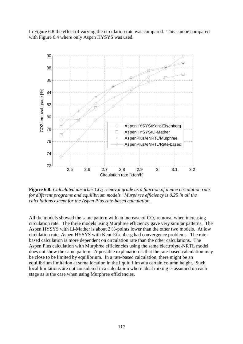
117

In Figure 6.8 the effect of varying the circulation rate was compared. This can be compared with Figure 6.4 where only Aspen HYSYS was used.

2.5 2.6 2.7 2.8 2.9 3 3.1 3.272

74

76

78

80

82

84

86

88

90

Circulation rate [kton/h]

CO

2 re

mov

al g

rade

[%

]

AspenHYSYS/Kent-Eisenberg

AspenHYSYS/Li-Mather

AspenPlus/eNRTL/Murphree

AspenPlus/eNRTL/Rate-based

Figure 6.8: Calculated absorber CO2 removal grade as a function of amine circulation rate for different programs and equilibrium models. Murphree efficiency is 0.25 in all the calculations except for the Aspen Plus rate-based calculation. All the models showed the same pattern with an increase of CO2 removal when increasing circulation rate. The three models using Murphree efficiency gave very similar patterns. The Aspen HYSYS with Li-Mather is about 2 %-points lower than the other two models. At low circulation rate, Aspen HYSYS with Kent-Eisenberg had convergence problems. The rate-based calculation is more dependent on circulation rate than the other calculations. The Aspen Plus calculation with Murphree efficiencies using the same electrolyte-NRTL model does not show the same pattern. A possible explanation is that the rate-based calculation may be close to be limited by equilibrium. In a rate-based calculation, there might be an equilibrium limitation at some location in the liquid film at a certain column height. Such local limitations are not considered in a calculation where ideal mixing is assumed on each stage as is the case when using Murphree efficiencies.

118

In Figure 6.9, the effect of varying the number of stages is compared. This can be compared with Figure 6.5 where only Aspen HYSYS was used.

7 7.5 8 8.5 9 9.5 10 10.5 11 11.5 1276

78

80

82

84

86

88

Number of stages

CO

2 re

mov

al g

rade

[%

]

AspenHYSYS/Kent-Eisenberg

AspenHYSYS/Li-MatherAspenPlus/eNRTL/Murphree

AspenPlus/eNRTL/Rate-based

Figure 6.9: Calculated absorber CO2 removal grade as a function of number of stages for different programs and equilibrium models. Murphree efficiency is 0.25 in all the calculations except for the Aspen Plus rate-based calculation. All the models showed the same pattern with increased CO2 removal with increased number of stages. The three models using Murphree efficiency gave very similar patterns. The Aspen HYSYS with Li-Mather is also here about 2 %-points lower than the other two models. The rate-based calculation is less dependent on the number of stages than the other calculations. This may be explained by that the rate-based calculation is close to be limited by equilibrium at this circulation rate as mentioned in the discussion after Figure 6.8 This explanation is however not supported by the Aspen Plus calculations with Murphree efficiencies and the same electrolyte-NRTL model which shows no such limitation. In Figure 6.10, the effect of varying the temperature in the inlet gas (and also the inlet liquid) is compared. The inlet liquid and inlet gas temperatures were specified to be equal.

119

30 32 34 36 38 40 42 44 46 48 5080

81

82

83

84

85

86

87

88

89

Temperature inlet [C]

CO

2 re

mov

al g

rade

[%

]

AspenHYSYS/Kent-Eisenberg

AspenHYSYS/Li-Mather

AspenPlus/eNRTL/Murphree

AspenPlus/eNRTL/Rate-based

Figure 6.10: Calculated absorber CO2 removal grade as a function of inlet gas and liquid temperature for different programs and equilibrium models. Murphree efficiency is 0.25 in all the calculations except for the Aspen Plus rate-based calculation. All the models showed the same pattern with decreased CO2 removal grade when increasing the inlet temperature. The three models using Murphree efficiency gave similar patterns. The deviation between Aspen HYSYS with Li-Mather and the two other Murphree efficiency models is between 1 and 3 %-points. The deviation increases with increasing temperature. The rate-based calculation is less dependent on inlet temperature than the other calculations, and this dependency is probably more reasonable. This is expected because the other models have been calculated with a constant Murphree efficiency, and the Murphree efficiency is expected to increase with increasing temperature.

6.3.3 Comparison of CO 2 removal simulations with other tools One of the few references comparing different simulation programs with pilot plant data for CO2 removal from atmospheric gas is Luo et al. (2009). They tested Aspen RadFrac, ProTreat, ProMax, Aspen RateSep, CHEMASIM from BASF and CO2SIM from SINTEF/NTNU. They concluded that basically all the codes were capable of giving reasonable predictions on overall CO2 absorption rate. The reboiler duties, the temperature profiles and concentration profiles were less well predicted.

120

In calculations from a PhD Thesis of Kothandaraman (2010), Aspen Plus calculates typically 4.3 MJ/kg CO2 removed when using an equilibrium based model and 4.5 MJ/kg CO2 when a rate-based model is used. This is more than calculated with the Kent-Eisenberg model or Li-Mather model in Aspen HYSYS. This is expected with a standard electrolyte-NRTL parameter set. With other electrolyte-NRTL parameters, e.g. from Liu et al. (1999) the calculated heat consumption will probably be less. The rate-based model in Aspen Plus is more difficult to converge than the equilibrium based models. It is more difficult to achieve a closed process with reasonable energy consumption using Aspen Plus than e.g. Aspen HYSYS. Convergence in the recycle calculation connecting the lean amine from regeneration to the lean amine to the absorption column is more difficult. One explanation for this is that the electrolyte-NRTL equilibrium model in Aspen Plus is more detailed than the models in Aspen HYSYS. At Telemark University College, the process simulation program ProMax has been tested in a number of student projects (Munasinghe, 2009; Madsen 2010). The equilibrium models used in ProMax were a Kent-Eisenberg model and an electrolyte-NRTL model, but they are probably not equivalent to the models used in Aspen HYSYS and Aspen Plus. The results were comparable with similar calculations in Aspen HYSYS, but there were some deviations. The ProMax calculations were performed with a constant Murphree efficiency, even though the ProMax documentation recommends a rate-based model. Calculations with ProMax and the electrolyte-NRTL model gave higher CO2 removal efficiency than other models. In her Master Thesis work, Madsen (2010) performed comparisons between calculations in Aspen HYSYS, Aspen Plus and also ProMax. The results from this work and the work of Madsen are similar. In her Aspen Plus calculations with Murphree efficiencies, EM = 0.25 was used for all components, not only CO2. Because of this, the temperature profiles looked slightly different. Madsen used a reaction condition factor 0.2 and film discretization factor 2, which also give slightly different results. The temperature profiles calculated with ProMax were closer to the rate-based calculations than the profiles calculated with Murphree efficiency and Aspen HYSYS or Aspen Plus in Figure 6.7. It is not obvious whether a Murphree or rate-based calculation of CO2 removal is most accurate. It does not look like differences in equilibrium models influence much on the parameter calculations. A rate-based calculation will probably give a more accurate detailed description of the process. An equilibrium based calculation is simpler and more robust. It is not clear whether any of the available tools are really predictive for CO2 absorption without any adjustable parameters. Careful comparisons and fitting of different tools to large scale experimental data are necessary to conclude about which tools are most accurate.

6.3.4 Calculation of water wash above CO 2 absorption section There are very few references to calculations of the water wash above the CO2 absorption section. Especially, there are very few references to the calculation of the MEA content in the gas from the CO2 absorption section. One reference is the CCP report (Choi, 2005) who claims that there is about 500 ppm MEA from the absorption section. In the NVE report, it is stated (Svendsen, 2006) that typical MEA content in this stream is 125 ppm. At Telemark University College, this has been evaluated in some Master Thesis projects, especially Munasinghe (2009).

121

The MEA content in the gas from the CO2 absorption section is a result of the Aspen HYSYS and Aspen Plus calculations in the subsections 6.3.1 and 6.3.2. The numbers here are from the base case calculations with 40 ºC in inlet gas and liquid temperature. The result from the Aspen HYSYS calculation was 352 ppm using Kent-Eisenberg and 349 ppm using the Li-Mather model. The results from the Aspen Plus calculations using electrolyte-NRTL was 75 ppm in the calculation with Murphree efficiencies and 71 ppm using the rate-based model. In Section 3.9 a value of the MEA concentration above a 30 wt-% MEA solution with CO2 loading 0.25 was estimated to approximately 60 ppm. When calculating amine loss (especially MEA loss) from the CO2 absorption section, an equilibrium model for MEA in gas and liquid is necessary. An electrolyte based model should be suitable for this. The only models in the simulation programs tested which have given reasonable MEA concentration out from the CO2 absorber section are the electrolyte based models like electrolyte-NRTL. Due to this, it is assumed that the MEA content out from the absorber section is in the order of magnitude 100 ppm as calculated by the Aspen PLUS program. The MEA amount from the absorption section increases with temperature. Calculation of the equilibrium in the water wash section must be based on a solubility of the amine (e.g. MEA) in water. This can probably be adequately described by a temperature dependent Henry’s constant as described in Section 3.9. The equilibrium concentration of MEA in the gas above a water solution may be so low that it can be assumed to be 0. In that case, the absorption in the water wash section is rate limited. If the equilibrium concentration of MEA above the wash water is some ppm, the wash water section will bring the MEA concentration down towards this value. The CO2 absorption column and the water wash column can be calculated in a process simulation program as one or two columns. In practice, the CO2 absorption and water wash sections will probably be in one column with constant diameter. If the two sections are calculated as one column, the same equilibrium model must be used. In Aspen Plus, the electrolyte-NRTL model can be used. Aspen HYSYS calculates an MEA equilibrium concentration that is much too high in the gas from the CO2 absorption section. It is then difficult to find a consistent way to calculate the water wash section because the input concentration is wrong. The mass transfer number (kG) for the water wash section has been estimated in Section 4.8.3 to be 0.034 m/s. Using Equation 5.10 with gas velocity 3 m/s, nominal packing area 250 m2/m3 and effective area 0.75, this results in a mass transfer HTU equal to 0.47 m. A packing height of ln(100) times HTU (approximately 2.2 m) will reduce the MEA concentration to 1 % of its value from the CO2 absorption section assuming that the equilibrium partial pressure of MEA is 0. With some safety margin, a reasonable packing height is then 3-5 m to reduce the order of magnitude concentration of MEA from 100 ppm to about 1 ppm above the equilibrium concentration. An uncertainty is the MEA in droplet form, which is difficult to estimate and difficult to remove.

122

6.4 Process simulation with varying Murphree effici ency

6.4.1 Aspen HYSYS simulation with varying Murphree efficiency Most of the Aspen HYSYS calculations have been performed with a constant Murphree efficiency. In the SIMS paper (presented in Section 6.2) a Murphree efficiency of 0.25 for each stage was used, and in the TCCS paper (Øi et al., 2009), a Murphree efficiency of 0.15 for each meter of packing was assumed. In Chapter 5, Murphree efficiencies for 1 meter of packing were calculated as a function of temperature at top and bottom conditions and the results were shown in Figures 5.2 and 5.3. In the poster presentation in Regina (Øi, 2009b), the estimated efficiencies were slightly different. The base case simulation in Section 6.2 has been calculated in Aspen HYSYS with Murphree efficiencies estimated in Figure 5.2 and 5.3. The inlet temperatures were 40 ºC, the top stage temperature was 49 ºC and the bottom stage temperature was 43 ºC. EM for 49 ºC at top conditions and EM for 43 ºC at bottom conditions were specified first. EM was kept constant down to the stage with maximum temperature (stage 4). Between the maximum temperature stage and the bottom stage, the EM was specified to vary linearly. In the Aspen HYSYS calculation, this resulted in a slightly different temperature profile, and the specified efficiencies were adjusted to be consistent with the new temperatures. By trial and error it was found that 13 stages (meter) were necessary to achieve 85.7 % removal with an inlet temperature of 40 ºC. With 12 stages (meter), a removal grade of 84.0 % was achieved. The results are presented in Table 6.2. The base case was also calculated with the automatic Aspen HYSYS estimation of plate efficiencies. It was necessary with 29 plates where the plate efficiencies varied from 0.096 in top to 0.051 in bottom. The efficiency was approximately constant down to the stage with highest temperature (stage 5) which had an efficiency of 0.101. This shows that the assumption of a constant efficiency down to the maximum temperature stage is reasonable.

6.4.2 Optimizing inlet temperature using varying Mu rphree efficiencies The temperature in the gas (and liquid) inlet was varied to find the maximum column efficiency or the minimum column height in the absorption column. The reaction rate is favoured by high temperature, but the CO2 absorption equilibrium is favoured by low temperature. The calculated Murphree efficiencies as a function of temperature were specified in the Aspen HYSYS calculation at inlet gas temperatures between 30 and 40 ºC. The procedure was repeated for gas inlet temperatures at 30 ºC and 35 ºC, and then 33 ºC and 34 ºC. For all these calculations, the maximum temperature appeared on stage 4 from above. The results are given in Table 6.2. Table 6.2: Aspen Hysys calculations at different input gas (and liquid) temperatures. Inlet temperature, ºC TBTM EM,BTM TTOP EM_TOP NSTAGES CO2 removal, % 30 35.2 0.103 40.9 0.215 12 85.45 33 37.4 0.108 43.3 0.222 12 85.50 34 38.4 0.110 43.9 0.226 12 85.80 35 39.0 0.111 44.8 0.229 12 85.67 40 42.1 0.118 48.5 0.240 12 84.00 40 42.7 0.119 49.0 0.243 13 85.69

123

As can be seen from Table 6.2, the column efficiency is highest at 34 ºC. Based on these calculations, the temperature giving the lowest necessary column height is 34º C, and the necessary column height is 12 meter. In a conference poster presentation in Regina (Øi, 2009b) a similar result was found using slightly different Murphree efficiencies. In that case an optimum inlet gas temperature was found at 33 ºC, giving 12 m of packing height necessary to achieve 85 % CO2 removal. The results in Table 6.2 have been based only on calculation of the absorption column. It is also tried to calculate the heat consumption as a function of inlet temperature. Similar parameter variations of other parameters were performed in Subsection 6.2.4. The regeneration process is not influenced much by the temperature in the absorption column. But because the amount of CO2 absorbed decreases with increasing temperature, the heat consumption per kg CO2 decreases slightly with temperature. To calculate the CO2 removal grade and heat consumption as a function of the inlet temperature with varying Murphree efficiency, a model developed by Kallevik (2010) was used. This is a further development of the Aspen HYSYS model presented in Section 6.2, and Figure 6.12 shows a flowsheet of the model. This flowsheet includes a direct contact cooler between the fan and the absorption column. The flowsheet includes automatic adjustment to a specified temperature difference (here 10 K) in the rich/lean amine heat exchanger. The make-up water and make-up amine is calculated from the losses, and the recycle to the absorption column is robust. The calculated CO2 removal grade and heat consumptions for 13 stages are shown as a function of inlet temperature in Table 6.3 and Figure 6.12. Murphree efficiencies were specified as discussed in Subsection 6.4.1.

Figure 6.11: Aspen HYSYS flowsheet of CO2 removal (Kallevik, 2010).

124

Table 6.3: CO2 removal and heat consumption as a function of inlet temperature to absorber calculated by HYSYS using variable Murphree efficiencies for 13 stages. Inlet temperature TTOP EM,TOP TBTM EMBTM CO2 removal, % QREBOILER 30 41.0 0.215 33.9 0.102 87.4 3.60 35 44.7 0.229 38.4 0.112 88.1 3.60 40 48.5 0.241 42.1 0.118 86.9 3.61 45 52.0 0.253 46.2 0.125 84.3 3.63 50 55.3 0.266 50.8 0.138 82.0 3.74 The calculations show a maximum CO2 removal efficiency at approximately 35 ºC. This is close to the optimum calculated earlier to 33 and 34 ºC.

30 32 34 36 38 40 42 44 46 48 5080

85

90

Temperature inlet [C]

(o)

CO

2 re

mov

al g

rade

[%

]

30 32 34 36 38 40 42 44 46 48 503.6

3.7

3.8

(*)

Hea

t co

nsum

ptio

n [M

J/kg

CO

2]

Figure 6.12. CO2 removal grade and heat consumption for 13 meter packing as a function of temperature with varying Murphree efficiencies. It was also tried to find the optimum inlet temperature using the automatic estimation of Murphree tray efficiency in Aspen HYSYS. The necessary number of trays at 34 ºC was 27 stages which achieved 84.9 % CO2 removal. When the temperature was varied from 25 to 40 ºC, the removal efficiency varied from 85.5 to 83.7 with the highest efficiency at the lowest temperature. This shows that when using the automatic Murphree tray efficiency calculation in Aspen HYSYS, the optimum temperature is as low as possible. This is however not expected to be realistic because the Murphree tray efficiencies calculated automatically by Aspen HYSYS are not expected to be accurate.

125

Similar calculations of inlet temperature have also been performed with Aspen Plus. In the case of Murphree efficiencies from Figure 5.2 and 5.3, the optimum inlet temperature was calculated to 29 ºC. The optimum temperature was found to be very dependent on the circulating rate. A weakness with this calculation is that there is one equilibrium model in the Murphree efficiency calculations (Kent-Eisenberg) and another (electrolyte-NRTL) in the absorber calculation. This may lead to inconsistencies. In Figure 6.10, a temperature dependence of rate-based calculation using Aspen Plus was shown. This shows an optimum CO2 removal grade at the lowest temperature at 30 ºC. The different programs and models give relatively large deviations in the calculated optimum of the inlet temperature. As seen from e.g. Table 6.2, the optimum is quite flat. This optimum is possible to find experimentally if the CO2 content in the outlet gas is measured carefully as a function of inlet temperature in a high absorption column. The economical optimum is probably higher than the temperature giving highest efficiency due to the cost of gas cooling. This optimum will probably be a result of a trade-off between cooling cost and equipment cost in the absorber.

6.4.3 Temperature profiles with varying Murphree ef ficiency and rate-based

0 2 4 6 8 10 12

36

38

40

42

44

46

48

50

52

54

56

Stage number from top (packing height)

Tem

pera

ture

[C

]

AspenHYSYS/Kent-Eisenberg/Tin=33 C

AspenPlus/eNRTL/Rate-based/Liq/Tin=33 C

AspenPlus/eNRTL/Rate-based/Vap/Tin=33 CAspenHYSYS/Kent-Eisenberg/Tin=40 C

AspenPlus/eNRTL/Rate-based/Liq/Tin=40 C

AspenPlus/eNRTL/Rate-based/Vap/Tin=40 C

Figure 6.13: Calculated absorber temperature profiles for varying Murphree efficiency using Kent-Eisenberg compared to rate-based simulation using electrolyte-NRTL.

126

The base case simulation with inlet temperature 40 ºC was calculated in Aspen HYSYS with Murphree efficiencies estimated from Figure 5.2 and 5.3, resulting in 85.7 % removal with 13 stages. 12 stages resulted in a removal grade of 83.5 %. The temperature giving the maximum absorption efficiency of 85.5 % was 33 ºC. The temperature profiles for these two cases are compared with rate-based calculations in Figure 6.13. The rate-based calculations were performed with 12 stages similar to the Aspen Plus calculations with 10 stages in Section 6.3. The parameters used were similar, except that the mixed flow stage model was used in the simulations with 12 stages due to easier convergence. The removal grade was 81.7 % at 40 ºC and 84.0 % at 33 ºC. At this amine circulation rate, the Aspen Plus rate-based simulation has difficulties in achieving 85 % removal grade, even with 12 stages each with 2 meter height. The absorber height in the rate-based calculations is considerably higher (24 meter) than in the calculations based on Murphree efficiencies (12 meter with efficiencies for 1 meter packing height). The temperature profiles using varying Murphree efficiency and rate-based simulation are very close. The largest deviation is that the rate-based calculations have a maximum temperature approximately 2 ºC higher than the calculations based on Murphree efficiencies. It is interesting to compare Figure 6.13 with Figure 6.7 where the Murphree efficiency is constant (0.25) at all (10) stages. Also in this figure, the deviation in maximum temperature is approximately 2 ºC. But the temperature profiles are much closer especially in the lower part of the column when using varying Murphree efficiencies.

6.5 Process simulation of CO 2 removal with other amines than MEA

6.5.1 CO2 removal with other amines than MEA using Aspen HYS YS CO2 absorbed in a mixture of MEA and water results in a high heat of absorption. This heat of absorption must be added in the regeneration to recover CO2. At high pressures, it is experienced that other amines can obtain lower heat consumption. This is claimed to be possible also at atmospheric conditions, e.g. by using the hindered amine solvent KS-1 as mentioned in Section 2.2. In this Section, it is tried to calculate the heat of absorption of CO2 removal using other amines than MEA. Diethanolamine (DEA) is much used for CO2 removal at high pressures. In the Aspen HYSYS program documentation, there is an example calculation (in a sample file folder) with DEA in a high pressure process. Aspen HYSYS absorber calculations have been performed at atmospheric conditions. A process with both absorption and desorption has been simulated, and the energy consumption becomes very large. The estimated Murphree efficiencies calculated by Aspen HYSYS are much lower than for MEA. The energy consumption is an order of magnitude higher than with MEA even when several stages with Murphree efficiencies of 1.0 are specified. Methyldiethanolamine (MDEA) in water is a popular solvent for CO2 absorption at high pressures because it results in reduced heat consumption in the stripper. When calculated at

127

atmospheric conditions in Aspen HYSYS, the estimated Murphree efficiencies were very low. The order of magnitude estimated by Aspen HYSYS for each plate was 1 %. Also with MDEA the energy consumption becomes very large in an absorption/ desorption process, even with Murphree efficiency specified to 1.0 in the absorber. A mixture of MEA and MDEA in water was also simulated with Aspen HYSYS at atmospheric conditions. When using amine mixtures, the Li-Mather model is recommended from the Aspen HYSYS documentation. Compared to using only MEA, the removal efficiency decreased and the energy consumption increased. Even though this is a much studied system, it is difficult to find an example in the literature of a calculated absorption/desorption process demonstrating this process for atmospheric absorption.

6.5.2 CO2 removal with other amines using other calculation tools In Aspen HYSYS, AMP (2-amino-2-methyl-1-propanol) and piperazine (PZ) are available components, but they are not components in the amine package. It is not expected that process simulation in Aspen HYSYS will give reliable results for a CO2 removal process with these components. There have been performed many simulations of CO2 removal into different amine mixtures at high pressures. Aruna et al. (2002) simulated CO2 removal into blends of AMP and MDEA. Mofarahi et al. (2008) have simulated an atmospheric CO2 absorption and desorption process for the amines MEA, DEA, MDEA and diglycolamine (DGA) using Matlab with a Kent-Eisenberg equilibrium model. In their calculations, a Murphree efficiency was specified to 35 % for each tray, and this is regarded as very optimistic. A CO2 absorption process into AMP at atmospheric conditions has been simulated by Gabrielsen et al. (2007) using Matlab as a tool. It was compared to performance data from the absorption part of a pilot plant. Kvamsdal et al. (2011) have simulated CO2 absorption into the solvent Cesar1 which is a mixture of AMP and piperazine. The in-house program CO2SIM was used to compare with performance data from the Esbjerg pilot plant which achieved a heat consumption as low as 2.9 MJ/kg CO2.

6.5.3 Questions to claimed potential in improved so lvents There are much resources spent on finding alternative solvents to MEA. MEA is however still the most referenced solvent for CO2 absorption at atmospheric pressure. Oexmann and Kather (2010) have written a paper where they are sceptical to the focus on low heat of absorption. They claim that a process with a solvent with a high heat of absorption (like MEA) may use less energy than a low heat of absorption solvent under practical conditions for CO2 removal at atmospheric pressure. High reaction rates and high temperature dependencies on CO2 capacity are typical advantages for solvents with a high heat of absorption. It is claimed by many that other solvents than MEA will have a lower regeneration energy for CO2. There are very few documented calculations of CO2 absorption from atmospheric gas including regeneration which demonstrates a calculated regeneration energy for any other solvent than MEA.

128

6.6 Dimensioning of equipment for cost estimation

6.6.1 Background for dimensioning of equipment for CO2 removal Description of the principles for general dimensioning and cost estimation based on a flowsheet calculation is given in Sections 2.8 and 2.9. As mentioned in Subsections 2.9.2 and 2.9.3, there are few open references on the dimensioning of CO2 removal plants. Most of the work done on this topic is not open information. Some details on the dimensioning of a standard CO2 removal plant are given in a report from SINTEF (Kvamsdal et al., 2005). Other sources which give detailed values for dimensioning of CO2 absorption processes are Abu-Zahra et al. (2007b) and Peeters et al. (2007). At Telemark University College, several student projects have dimensioned CO2 removal plants based on these principles using Aspen HYSYS as the main tool (e.g. Hansen et al., 2005; Amundsen et al., 2007).

6.6.2 Specifications for equipment dimensioning of standard case A poster was presented at the TCCS conference in Trondheim (Øi et al., 2009) based on the results from the Master Thesis of Blaker (2008). The main specifications for the sizing calculations were:

- Heat transfer number in rich/lean exchanger: 500 W/(m²·K) - Murphree efficiency per meter packing height: 15 % - Gas velocity in absorption column: 3 m/s - Wall thickness in columns: 0.01 m

500 W/(m²·K) was selected as a typical number for the rich/lean heat exchanger. Kvamsdal et al. (2005) used 550 W/(m²·K) for a shell and tube rich/lean heat exchanger. 15 % Murphree efficiency was estimated for 1 meter of structured packing compared to 25 % which was regarded as optimistic in earlier calculations. 15 % is a value between typical top and bottom conditions in Figure 5.2 and 5.3. Shell and tube heat exchangers were assumed, and structured packing was assumed in the absorption column. Other specifications and choices are given in the Thesis report (Blaker, 2008). Based on this, dimensioning factors were calculated like area for heat exchangers, capacity and outlet pressure for pumps and mass of steel for columns.

6.7 Process simulation including cost estimation an d optimization

6.7.1 Background for simulation and cost estimation of CO 2 removal In this work, all the equipment cost estimation has been based on open-source correlations or commonly used programs. Estimated values for process equipment are most often found for carbon steel (CostPURCHASE,CS). Installed cost for each item have then been calculated by multiplying with a type and size dependent installation factor (fTOT,CS) and adjusted for material with a material factor (fMAT) as shown in Equation (6.1).

129

)]1f(f)1ff[(CostCost PIPEMATPIPECS,TOTCS,PURCHASEINSTALLED +⋅+−−⋅= (6.1)

The total installation factor is the sum of factors for the equipment, installation, piping, electric, instrument, civil, steel and concrete, engineering, procurement, project control, site management, project management, administration, commissioning and contingency. In most of this work, the total installation factors and piping factors are estimated as a function of equipment cost, e.g. from Table 6.3. The original table from Eldrup can be found in Blaker (2008). In e.g. Table 6.4, it is seen that the most expensive equipment units have typical installation factors (Lang factors) between 3 and 7. Table 6.3: Installation factors and piping factors as a function of equipment cost in carbon steel based on a table from Eldrup (Blaker, 2008). Equipment cost (CS)

Installation factor, [f TOT,CS]

Piping-factor [f PIPE]

[kNOK]

100-500 6.81 0.79 500-1000 5.41 0.58

1000-2000 4.64 0.46 2000-5000 3.85 0.34

5000-15000 3.5 0.29 >15000 2.8 0.21

6.7.2 Cost estimation and optimization results for standard case The basis for the process presented at the TCCS conference in Trondheim (Øi et al., 2009) was close to the process specified in Table 6.1. The exhaust gas flow was 110 000 kmol/h, the CO2 content in the exhaust was 3.7 mol-% and the water content was 7.8 mol-%. The basis for the dimensioning was presented in Section 6.6. Equipment cost estimates for a base case were calculated using an open available cost estimation calculator on internet (Peters et al., 2008). Installed cost in carbon steel for each item was calculated by multiplying with a size dependent installation factor from Table 6.3. A spreadsheet integrated in Aspen HYSYS calculated equipment cost, installed cost (investment) and energy cost (operating cost). Optimum (net present value) was found from a series of calculations. For the base case conditions, the installed cost was estimated to 790 mill. NOK (160 mill. USD) and the energy cost (10 years calculation period) to1860 mill. NOK (370 mill. USD). The values are from 2007 when 1 USD was close to 5 NOK.

130

Table 6.4: Overview over installed cost including installation factors for CO2 removal plant from natural gas besed power plant exhaust (Øi et al., 2009).

Eq. cost CS - 2007

Material type

Material factor

Inst. factor CS

Piping-factor Eq. factor Inst.

factor Installed cost (2007) Equipments

[kNOK] [kNOK] [kNOK] Flue Gas Blower 41399 SS 304 - 2.8 - - - 115916 DCC 16629 Exotic 2.5 3.5 0.29 1 5.435 90378 Absorber 64592 SS 316 1.75 2.8 0.21 1 3.707 239473 Rich Pump 2272 SS 304 - 3.85 - - - 8749 Rich/Lean Hx 1143 SS 316 1.75 4.64 0.46 1 5.735 213171 - - Desorber 9955 SS 316 1.75 3.5 0.29 1 4.467 44473 Reboiler 7589 SS 316 1.75 3.5 0.29 1 4.467 33903 Lean Pump 3568 SS 304 - 3.85 - - - 13738 Lean Cooler 2028 Exotic 2.5 3.85 0.34 1 5.86 11886 Condenser 120 Exotic 2.5 6.81 0.79 1 9.495 1137 CO2 Cooler 1398 Exotic 2.5 4.64 0.46 1 6.83 9546 Separator 392 SS 316 1.75 6.81 0.79 1 8.152 3194

Total installed cost for listed equipment [kNOK] 785565

The estimate did not include CO2 compression, storage, transport, water wash, reclaiming or utility systems. Energy cost (heat and fan power) was net present value over 10 years in full operation (8000 h/yr), other operating costs were neglected. The absolute value of the total estimate is not expected to be very accurate, but it is expected to include most of the cost factors that varies with size and capacity. Column height, minimum temperature difference in the lean/rich heat exchanger and gas inlet temperature were then varied. CO2 removal grade was kept at 85 % in most of the simulations. Cost change of installed equipment from base case to new conditions was calculated by multiplying with the capacity ratio raised to 0.65. Cost for other conditions than the base case, were calculated using the same installation factors as in the base case. When calculating the optimum inlet temperature, the Murphree efficiency was specified to increase with 0.01 per 10 K so that the efficiency was 0.145 at 35 ºC. The results are shown in Table 6.5.

131

Table 6.5: Calculated optimum process parameters for CO2 removal process with 85 % removal grade and 10 years calculation period.

Parameter Optimum value Comments

Absorption packing height[m] 16 EM = 0.15

Minimum ∆T [ºC] 19 Cold side of lean/rich heat exchanger

Inlet gas temperature [ºC] 35 EM varies with temperature Figure 6.14 shows net present value as a function of minimum ∆T in rich/lean heat exchanger.

520

530

540

550

560

570

580

590

5 10 15 20 25 30

Delta T [ oC]

(Neg

ativ

e) N

et P

rese

nt V

alue

[mill

. U

SD

]

Figure 6.14: Net present value as a function of minimum ∆T in lean/rich heat exchanger (Øi et al., 2008). Net present value for different removal rates were calculated for different values of removed CO2. Optimum removal grade was calculated when captured CO2 had a specified value. With a value of 300 NOK/ton (60 USD/ton) the optimum was 82 % CO2 removal. With a value of 600 NOK/ton (120 USD/ton) the optimum was 85 % CO2 removal. Automatic optimization is possible in Aspen HYSYS using the Optimizer tool. Minimum temperature difference in heat exchangers was then calculated to 17.7 ºC compared to 19 ºC manually. Optimum removal rate if captured CO2 had a specified value equal to 300 NOK/ton was 81.8 % compared to 82 % manually and with a value of 600 NOK/ton 84.3 % compared to 85 % manually. One explanation for the differences is that there are some tolerances in the material and energy balances in the Aspen HYSYS calculations. If the tolerances are made smaller than the default values, the values calculated automatically and manually are expected to be closer.

132

6.7.3 Comparisons with other cost optimization calc ulations Kallevik (2010) at Telemark University College has performed cost estimation of CO2 removal based on Aspen HYSYS simulations in his Master Thesis. Heat transfer numbers and column gas velocities were estimated to slightly higher values compared to the values in Subsection 6.6.2. Kallevik used equipment cost data from the textbook by Smith (2005). Cost of installed equipment was estimated using Equation (6.1) and with type and size dependent installation factors. Electricity cost was set to 0.4 NOK/kWh, and steam cost was set to 0.1 NOK/kWh. The parameters presented in Table 6.5 were optimized with these new specifications. The calculated cost optimum temperature difference in the rich/lean heat exchanger was between 12 and 14 ºC. The optimum absorber packing height at 85 % CO2 removal was calculated to 15 m. The cost optimum gas inlet temperature was calculated to approximately 40 ºC. The values between 35 and 40 ºC were not calculated, and might be more optimal. The optimum values calculated by Kallevik were in the same order of magnitude compared to the values in Table 6.4. The deviation is largest in the optimum temperature difference in the rich/lean heat exchanger. In the CCP project (Choi et al., 2007), a minimum temperature difference of 11 ºC was used in the calculations. It was based on shell and tube heat exchangers, and the temperature difference was claimed to be close to cost optimum. In the same report, it is suggested to change to plate exchangers in order to reduce the cost. This will probably reduce the optimum temperature difference. The optimum temperature difference in the rich/lean exchanger is very dependent on the ratio of heat exchanger cost and energy cost.

6.7.4 Simultaneous cost optimization of several par ameters There are several parameters that can be optimized. In an optimization calculation, it is normal to keep all other parameters constant. It is a challenge to optimize all the parameters in the CO2 removal process to achieve a total cost optimum process. Only ∆TMIN (in practice between the hot and cold streams at the cold end of the rich/lean heat exchanger) has been optimized automatically (Blaker, 2008; Øi et al., 2008). In principle, all parameters might be optimized simultaneously using e.g. the Optimizer tool in Aspen HYSYS. The main limitations for automatic calculations are in the column calculations. The first problem is the convergence problem in the columns. A limitation in Aspen HYSYS is that the number of stages in the columns must be specified before the optimization.

133

6.8 Optimizing CO 2 absorption using split-stream configuration

6.8.1 Split-stream principle and other process conf iguration options In a simple absorption and desorption process, the absorption liquid circulates as one single stream from the bottom of the absorption column to the desorption column, and from the bottom of the desorption column to the top of the absorption column. There are however possibilities to have multiple feeds or draws in both the absorption column and the desorption column. Such configurations are called split-stream or split-flow configurations. A simple example is shown in Figure 6.15. In addition to the rich and lean solvent streams, there is also a semi-lean stream which is partly regenerated.

Figure 6.15: Principle of split-stream configuration (Øi and Vozniuk, 2010). Different alternatives for the split-stream principle are explained in Kohl and Nielsen (1997) and in Polasek et al. (1982). A survey of process flowsheet modifications for CO2 removal is given by Cousins et al. (2011a). Energy efficient alternatives are lean amine flash and multiple pressures in the stripper (Oyenekan and Rochelle, 2006). Very few calculations of CO2 removal from exhaust gas based on split-stream have been found in the open literature. A paper by Aroonwilas and Veawab (2007) is one example, but the details in the calculations are not shown. Karimi et al. (2010) using the program Unisim and Cousins et al. (2011b) using Aspen Plus show process simulations of different split-stream configurations. It is known that engineering companies, especially Fluor, develop split-stream processes, but the results have not been published. The main advantage with a split-stream configuration, is a reduction in heat consumption in the stripper. One reason for the reduction in energy consumption is that only a part of the circulating liquid needs to be fully regenerated. Another explanation is that the driving force especially in the absorption column is reduced so that the thermodynamic losses are reduced. The main draw-back is a

134

more complex process. Due to reduced driving force in the absorption process, the absorption column normally has to be higher when using split-flow.

6.8.2 Split-stream simulation using Aspen HYSYS The flowsheet in Figure 6.16 with and without split-stream has been calculated with Aspen HYSYS version 7.0, and the amine package with the Kent-Eisenberg model was used. The calculation is based on the Master Thesis work of Vozniuk (2010) and the conference paper presented at the PTSE 2010 conference (Øi and Vozniuk, 2010). Input specifications for both the standard process and the split-flow process are given in Table 6.6.

Figure 6.16: Aspen HYSYS model for CO2 removal using split-stream configuration (Øi and Vozniuk, 2010). The calculation sequence was based on guessed (or specified) flow rates and compositions to the absorption column. The exhaust gas fan and the following cooler was calculated first. Then the absorption column was calculated with the modified HYSIM in and out solver method with adaptive damping. Then the rich amine pump and the rich side of a multistream heat exchanger were calculated before the stripper was calculated. Then the lean and semi-lean side of the multistream heat exchanger, the return pumps and the coolers were calculated. Then the concentrations of the lean and semi-lean streams were checked manually, and the specified concentrations were adjusted in the feed streams to the absorber. 18 stages was selected in the base case because a higher number only gave slightly reduced energy consumption. In the case of the split-stream base case, the energy consumption was reduced up to 24 stages. The semi-lean feed to absorber stage 21 was found to give the lowest energy consumption. In the base cases with minimum heat exchanger temperature difference 10 K, the energy consumption was calculated to 3.8 MJ/kg CO2 removed in the standard process and 3.4 MJ/kg with the split-stream configuration.

135

Table 6.6: Input specifications for Aspen HYSYS calculations with 85% removal efficiency and minimum heat exchanger temperature difference of 10 K (Øi and Vozniuk, 2010). Specifications Base case without split stream Base case with split stream

Inlet gas temperature [˚C] 40 40

Inlet gas pressure [bar] 1.11 1.11

Inlet gas flow [kmol/h] 110000 110000

CO2 in inlet gas [mole-%] 3.7 3.7

Water in inlet gas [mole-%] 7.8 7.8

Lean amine temperature [˚C] 40 40

Lean amine pressure [bar] 1.01 1.01

Lean amine rate [kmol/h] 148000 103500

MEA content in lean amine [mass-%] 29 29

CO2 in lean amine [mass-%] 5.5 5.5

Number of stages in absorber 18 24 (semi-lean to 21)

Murphree efficiency in absorber 0.15 0.15

Rich amine pump pressure [bar] 2 2

Heated rich amine temperature [˚C] 104.2 96.6

Number of stages in stripper 6+Condenser+Reboiler 6+Condenser+Reboiler

Murphree efficiency in stripper 1 1

Reflux ratio in stripper 0.1 0.1

Reboiler temperature [˚C] 120 120

Lean amine pump pressure [bar] 2 2

Semi-lean amine temperature [˚C] - 40

Semi-lean amine pressure [bar] - 1.11

Semi-lean amine rate [kmol/h] - 100000

MEA content in semi-lean amin [mass-%] - 28

CO2 in semi-lean amine [mass-%] - 9.1

6.8.3 Parameter variations The energy consumption can be reduced by increasing the number of stages in the absorption column. With the standard process and 10 K in minimum temperature difference, minimum energy consumption was 3.8 GJ/ton CO2 with 20 stages. With a split-stream configuration, an increase from 18 to 24 stages resulted in a reduction of energy consumption from 3.8 to 3.4 GJ/ton CO2. With 5 K temperature difference, the energy consumption has been reduced down to 3.0 MJ/kg CO2 with 26 stages in the absorber and the semi-lean stream feed at stage 21 from the column top. With 15 K in minimum temperature difference, a split-flow configuration did not give any energy reduction. To vary the minimum temperature difference, the temperature specification on heated rich amine to the stripper column was adjusted.

136

The semi-lean feed stage to the absorber column was varied in each calculation to find the optimum. The removal stage for semi-lean amine from the stripper was stage 4 from top in all the calculations. The lean and semi-lean amine flow rates were varied to maintain 85 % CO2 removal. The ratio between lean and semi-lean flow rate and the removal stage for semi-lean amine from the stripper column are parameters that can be further optimized.

6.8.4 Dimensioning and cost estimation of split-str eam process The specifications for dimensioning were more detailed than for the standard process in Subsection 6.6.2. The heat transfer number in the rich/lean exchanger was 500 W/(m²·K), in amine coolers and the reboiler 800 W/(m²·K) and in the condenser and CO2 cooler 1000 W/(m²·K). The heat transfer values are close to the values used by SINTEF (Kvamsdal, 2005) which were 550, 800, 1200, and 1000 W/(m²·K) for the rich/lean exchangers, coolers, reboiler and condensers, respectively. Murphree efficiency per meter absorber packing height was specified to 15 %. Packing height in water wash section was estimated to 5 meter. The absorber height in addition to packing was 12 m without and 14 m with split-stream and desorber height was 25 m without and 30 m with split-stream. Direct contact cooler dimensions were 15 m in diameter and 10 m in height. The diameters in the absorption and desorption columns were based on a gas velocity of 3 m/s and 1 m/s. The fan was specified as a radial centrifugal fan with electrical motor. The fan and the pumps were specified with 75 % adiabatic efficiency and with electrical motors. The heat exchangers (except the kettle type reboiler) were specified as floating head heat exchangers with ideal countercurrent flows. The multi-stream exchanger might actually be a system of traditional heat exchangers. The cost of the heat exchangers were estimated with heat exchanger areas as the dimensioning factor. The areas were calculated from heat duties and logarithmic mean temperatures from Aspen HYSYS combined with the heat transfer numbers. Structured packing was assumed in the absorption column. The cost of not listed equipment like filters, storage tanks and a reclaimer was neglected. The cost estimation was based on the equipment dimensions calculated from the principles in Section 6.6. The base case processes have been cost estimated by Vozniuk (2010) with basis in 2007 regulated to 2010 with Aspen ICARUS (version 16.0.0). Installed cost for each equipment unit was calculated as a product of equipment cost and a total installation factor as explained in Subsection 6.7.1. A structured packing with specific area 250 m2/m3 was specified in the columns. It was assumed that the packing cost was 1.4 times higher than the cost for 2” pall rings (calculated by Aspen ICARUS) as suggested by Duss et al. (1987).

137

Table 6.7: Equipment and installed cost for CO2 removal plant (Øi and Vozniuk, 2010).

Equipment list

Equ

ipm

ent c

ost,

base

ca

se [

1000

EU

R]

Equ

ipm

ent c

ost,

split

st

ream

[100

0 E

UR

]

Mat

eria

l typ

e

Mat

eria

l fac

tor

Tot

al in

stal

latio

n fa

ctor

, ba

se c

ase

Tot

al in

stal

latio

n fa

ctor

, sp

lit s

trea

m

Inst

alle

d co

st, b

ase

case

, [1

000

EU

R]

Inst

alle

d co

st, s

plit

stre

am [1

000

EU

R]

Flue gas blower 347 347 SS304 1.3 1.3 1.3 451 451

Fan motor 641 641 SS304 1.3 1.3 1.3 834 834

DCC 1777 1777 Exotic 2.5 5.43 5.435 9661 9661

Absorber skirt 2556 2926 SS316 1.75 3.71 3.71 9476 10848

Water wash skirt 1584 1584 SS316 1.75 4.47 4.47 7075 7075

Rich pump 249 363 SS304 1.3 1.3 1.3 323 472

Rich/Lean exch. 129 120 SS316 1.75 5.74 6.6 24064 41493

Desorber skirt 460 424 SS316 1.75 4.86 4.86 2235 2056

Reboiler 897 769 SS316 1.75 4.47 4.47 4007 3435

Lean pump 248 167 SS304 1.3 1.3 1.3 323 218

Lean cooler 251 179 Exotic 2.5 6.83 6.83 1716 1223

CO2 cooler 180 96 Exotic 2.5 6.83 7.78 1228 746

Condenser 33 33 Exotic 2.5 9.5 9.5 315 315

Separator 128 128 SS316 1.75 5.74 5.74 732 732

Absorber packing 25119 33492 SS316 - - - 25119 33492

Water wash packing 6977 6977 SS316 - - - 6977 6977

Desorber packing 960 688 SS316 - - - 960 688

Semi-lean pump - 167 Exotic 1.3 - 1.3 - 218

Semi-lean cooler - 179 Exotic 2.5 - 6.83 - 1223

Total 42536 51057 95494 122156

The operating cost was estimated from the energy cost. The electricity cost was specified to 0.05 EUR/kWh and the steam cost (130 ºC steam) was 0.013 EUR/kWh (approximately 25 % of the electricity cost). Operating time was 8000 hours per year and interest rate was 7 %. For a period of 10 years, the net present (negative) value of the energy consumption of the split-stream process was 109 mill. EUR compared to 127 mill. EUR for the standard process. The increase of the plant installed cost was 27 mill. EUR, so with 10 years pay-back time, the standard process without split-stream was most economical. The split-stream alternative becomes more attractive when the calculation period increases. If the period of calculation is set to 20 years, the reduction in operating cost increases to 27 mill. EUR, and with a calculation period above 20 years, the split-stream was most economical. The advantage with the split-stream alternative is sensitive to the energy cost. If the energy cost increases, the split-stream alternative becomes more attractive.

138

6.8.5 Conclusions and further optimization of split -stream configurations The Aspen HYSYS calulations have shown that it is possible to reduce the energy consumption considerably in a CO2 removal plant using a split-stream configuration. An energy consumption of 3.0 MJ/kg CO2 has been calculated using a simple split-stream configuration and 5 K temperature difference in the rich/lean heat exchanger. With 15 K temperature difference, a split-stream configuration has not demonstrated any reduction in the energy consumption. There are possibilities to optimize the absorption and desorption process further. Parameters like the ratio between lean and semi-lean flow-rate and the semi-lean removal stage from the desorber can be further optimized. However, the process complexity and capital cost may increase. The cost calculations of the base cases show that the simple split-stream is on the limit of being economically. The economical potential of further complexity is then doubtful. There are many other possibilities to improve the standard CO2 removal process than a split-stream configuration (Oyenekan and Rochelle, 2006; Cousins et al., 2011a). It is claimed by e.g. Karimi et al. (2010) that a simple lean amine flash with recompression has a large energy reducing effect compared to the necessary investment. It is also possible to combine multiple flashes with a split-stream configuration. To find an optimum process, calculations including cost estimation must be performed. The cost calculations in Section 6.7 show that the cost optimum temperature difference is probably higher than 10 K. The calculations in this work show that there is no energy improvement in a split-stream configuration when ∆T is as high as 15 K. This makes the economy of a split-stream process doubtful. The calculations performed here are based on CO2 removal from the exhaust from a natural gas based power plant with a low CO2 concentration. Use of a split-stream configuration will probably be more attractive with a more CO2-concentrated exhaust, e.g. from a coal based power plant.

6.9 Uncertainties in the simulation results

6.9.1 Uncertainties in the physical properties The accuracy in the process simulation calculations is dependent on the accuracy of the data on physical properties used. The accuracy in densities, transport properties and heat capacities are expected to have uncertainties within a few percent. The largest uncertainty in the physical properties is probably connected to the vapour/liquid equilibrium models. There is also an uncertainty in the heat of absorption (and desorption) of CO2 in the amine solution. This gives rise to differences in heat consumption and temperature profiles as shown in Figures 6.7 and 6.13. The difference in heat of absorption is in the order of magnitude 10 %.

139

6.9.2 Uncertainties in dimensioning The uncertainties in equipment dimensions (based on a flow diagrams after process simulation) are large. The selection of type of equipment and material is also of importance. In the case of the absorption column, a structured packing of stainless steel is expected to be the optimum choice. Random packing is cheaper, but will probably result in a more expensive overall solution. The packed section of the absorber column height is based on the stage efficiency which has an uncertainty of ± 40 %. As discussed in Chapter 5, the main uncertainty is probably in the efficient gas/liquid interfacial area. Other important uncertainty factors are the vapour/liquid equilibrium and whether the pseudo first order conditions are valid. The column diameter which is based on gas velocity has a lower uncertainty. If the column diameter is based on a pressure drop specification, the uncertainty will be higher. The uncertainty in the desorber column is of the same order of magnitude. The dimensioning factors in the heat exchangers are the heat transfer areas. With the assumption of a shell and tube heat exchanger, the uncertainty which is very dependent on the overall heat transfer number is assumed to be in order of magnitude ± 30 %. In some of the calculations, ideal countercurrent flow in the heat exchangers is assumed. This is normally only an approximation. To adjust for this, an adjustment factor (F-factor) can be used. Another way to adjust for this, is to use a conservative heat transfer number. The reboiler heat consumption is expected to be accurate within ± 10 %. The heat exchangers are in a large-scale amine plant expected to be plate exchangers. However, since the purpose of the dimensioning is to achieve a cost estimate, shell and tube exchangers in stainless steel can be a practical specification to achieve a reasonable cost estimate. It is more difficult to find general dimensioning and cost estimation methods for plate type heat exchangers. Sintef (Kvamsdal et al., 2005) has compared the cost of shell and tube and plate exchangers for an amine plant, and found that the use of plate exchangers gave a slightly reduced investment. The uncertainty in the cost of heat exchangers is large. Stainless steel has been chosen for most of the equipment. This increases the equipment cost to a factor of more than 2. For the total cost estimate, the choice of material is however not so important because most of the cost factors are not influenced by the choice of material.

6.9.3 Uncertainties in cost estimation The uncertainty in the cost estimation of the process equipment is large. After the type selection, dimensioning and choice of material, the uncertainty in the cost is of order of magnitude ± 50 %. The additional uncertainty is due to the choice of standards, local factors and differences between equipment suppliers. The most influencing part of the cost estimate is the packed section of the absorber. The uncertainty is especially high because there are few suppliers and different qualities. There are very few references on estimated cost of structured packing in large scale columns. One of the few is Duss et al. (1997) from Sulzer Chemtech who suggest to estimate the cost of the standard structured packing Mellapak 250Y in stainless steel 304 to 1.4 times the cost of 2 inch Pall rings. The uncertainty is increasing for high performance structured packing.

140

The installed equipment cost of the CO2 removal plant is dependent on additional factors. Quality levels for safety, environmental protection, reliability and monitoring will influence the total cost estimate. Also local conditions are very different. These factors may partly explain the different cost estimates varying from 0.5 billion NOK to 5 billion NOK for the investment of a plant for the removal of 1 mill. ton CO2 /yr. Dave et al. (2011) have compared estimated CO2 capture cost in projects in China and Australia. They concluded that in Australia the capital cost dominated, and in China the fuel cost dominated. The operating cost is dependent on the energy prices. The uncertainty in the energy consumption is much lower, so the uncertainty in operating cost is about proportional to the energy cost. Operating costs like salaries and maintenance are neglected in most of the calculations in this work. This could be included by estimating it to a percentage of investment cost. In the investment cost, there are factors that increase with capacity which are not included. In the operating cost, only energy cost is included. The factors which are not included are difficult to estimate accurately. Because of these factors, both investment and operating cost are probably underestimated. In this work, estimates for installed equipment without CO2 compression of 0.8 to 1.4 billion NOK have been calculated. This is equivalent to 60 to 110 mill. EUR. These estimates are regarded as reasonable for parameter optimization calculations.

6.9.4 Uncertainties in process parameter cost optim ums Process parameter cost optimums are of course dependent on the uncertainties in the cost estimation. However, the cost optimums of many of the parameters are not very much influenced of the large differences in cost estimates. The minimum temperature difference in the rich/lean heat exchanger has been calculated to values between 12 and 19 ºC. This value is very dependent on the ratio between investment and energy cost. Most of the calculations in this work have given an optimum between 12 and 15 ºC based on the assumption of shell and tube heat exchangers. The use of less expensive plate exchangers will probably reduce the optimum temperature difference. There is however a question whether the cost of the heat exchangers are actually over- or under-estimated. If a more expensive exchanger type than necessary is assumed, this will tend to over-estimate. If a simplified heat exchanger solution is assumed, this will tend to under-estimate. In this work, simplified solutions and shell and tube heat exchangers are assumed in most of the cost estimation calculations. It is not clear whether this leads to an over or under-estimation of the installed heat exchanger cost. The optimum rich loading is calculated to about 0.47. The optimum rich loading is connected to an optimized circulating rate. The optimum is close to the loading giving lowest heat consumption in the reboiler, and this is not influenced much by the uncertainties. The optimum gas temperature before absorption has been calculated to values between 35 and 40 ºC. In literature, values between 40 and 50 ºC are most often found, but there are no references to an optimized value. The optimum temperature is mostly dependent on the equilibrium and kinetic conditions, and is little influenced by the cost estimates. The optimum inlet temperature is of course also dependent on the temperature of the available cooling source.

141

7. Discussion

7.1 Accuracy in cost estimation of CO 2 absorption plants The purpose of the capital cost estimates in this work is to calculate optimum process parameters and not to estimate the absolute values of these estimates as accurate as possible. For the removal of a specified amount of CO2, the accuracy of the installed equipment cost or a turn-key plant is in the order of magnitude +100/-50 %. The possible differences in different specifications are important in this uncertainty. The estimate values on the total project investments including land, utility systems and other factors differ even more than this. It is outside the scope of this work to evaluate these differences. The estimates on operating cost of CO2 absorption plants also have large deviations. The largest influence on the operating cost is the energy consumption, and especially the heat consumption for the regeneration of CO2. The uncertainty in this heat consumption is low. The uncertainty in the total operating cost is almost proportional to the uncertainty in the value on this heat.

7.2 Limitations in the models

7.2.1 Limitations for pseudo first order assumption The traditional absorption conditions are according to the calculations in this work close to pseudo first order conditions below about 50 ºC. In the absorption column, this is in the normal temperature range for CO2 removal from a natural gas based power plant. The deviation in the estimated absorption rate at 50 ºC is estimated to be less than 10 %. For CO2 removal from a coal based power plant, the temperature can be higher. In the case of inlet temperatures of 40 ºC, only a small part of the absorption column will operate above 50 ºC. In that case, a pseudo first order assumption will not lead to serious deviations. For CO2 removal from exhaust gas from a natural gas based power plant, the optimum inlet gas temperature has been calculated in this work to be less than 40 ºC. In that case, the pseudo first order assumption is probably approximately valid for optimum conditions.

7.2.2 Limitations for Murphree efficiency estimatio n methods The accuracy of a calculated Murphree efficiency based on pseudo first order conditions is close to the accuracy of the calculated absorption rate. A constant temperature at a stage is also assumed. There might be a difference between the gas and liquid bulk temperature, and there might be a temperature gradient through the gas or liquid film. For temperatures up to about 60 ºC, the deviation from pseudo first order can be estimated using estimation methods. The most well-known methods are based on enhancement factors. When using such methods for the estimation of Murphree efficiencies, the uncertainty is estimated to be in order of magnitude 10 % up to about 60 ºC.

142

7.2.3 Limitations for penetration and surface renew al model Many of the rigorous models to calculate the absorption rate in CO2 absorbers are based on the penetration or the surface renewal model. These absorption models are regarded as more close to reality than film models based on diffusion. The time of surface exposure or the surface renewal rate are used as parameters in the models. These parameters are normally not known for a packed column. There are in general large uncertainties in the knowledge of the actual process of absorption followed by chemical reaction in industrial absorption columns. Some of the rigorous models in the literature are based on the discretization of the liquid films in thin layers. There is high uncertainty in whether this is a description close to reality.

7.3 Trade-offs in optimization of CO 2 absorption plants

7.3.1 General optimization of process parameters The purpose of this subsection is to discuss how to find the optimum process parameter values in an amine based CO2 removal plant. In most cases, by specifying optimum conditions, economical optimum is meant. But in some cases, optimum conditions can be found from energy evaluations. And in some cases, practical considerations also influence on the choice of parameters. A base case using MEA was specified with inlet gas stream and with specified CO2 removal. Other specifications are not regarded as important for parameter optimization, but specifications on MEA concentration in outlet exhaust gas and specification on MEA in product CO2 may also be relevant. Cost data on equipment, material selection, cost of energy, operation time and payback time are important background information for an optimization evaluation. The choice of process parameters which can be optimized are typically: - Gas temperature into absorption column (after cooling and possibly pressure increase in fan) - Temperature on amine solution to absorption column - Minimum temperature difference in rich/lean amine heat exchanger - Reboiler temperature (often specified to 120 ºC) in desorber - Condenser temperature (or reflux ratio) in desorber - Solvent circulation rate (or ratio of mole-flow CO2 to mole-flow MEA from absorber) - Pressure in desorber column - Pressure in gas to absorber (to overcome pressure drop in absorber) The parameters are chosen so that equipment can be dimensioned to achieve these process parameters. The idea is that a typical project will work out a flowsheet describing the process and defining the performance of each type of equipment. Then suppliers of equipment will suggest equipment that meets the specifications. The accuracy in the optimization of process parameters is dependent on the cost estimation of equipment and also on the cost estimation of installing the equipment. Other investment cost factors are not regarded as important for the process parameter optimization. Operating cost, where energy cost is largest, is also important.

143

There is not much found in the literature about systematic ways to find optimum process parameters. Only typical process values are normally mentioned. Abu-Zahra et al (2007a; 2007b) is one example of calculations of process parameters. Optimization in the operation phase will be slightly different compared to optimization in the design phase. In the case where the equipment dimensions are specified, energy optimization is a reasonable optimization criteria. Another possibility is to optimize the efficiency (e.g. the CO2 removal rate).

7.3.2 Inlet gas temperature. Typical values found in literature are between 40 and 50 ºC. Arguments for a low temperature:

- Higher CO2 capacity (from equilibrium) - Lower evaporation tendency of amine

Arguments for a high temperature:

- Lower cost in direct contact cooler - Higher reaction rate - Lower viscosity

The most important factors are probably the reaction rate and the equilibrium. In that case it is possible to calculate an optimum without any cost data. The optimum temperature will be the one giving the lowest column height. Such calculations have been performed, and the optimum was calculated to be between 33 and 35 ºC with Aspen HYSYS with Kent-Eisenberg or Li-Mather. The optimum was calculated to be lower with Aspen Plus and the electrolyte-NRTL model. A calculation also taking the cost in heat exchanger into consideration was performed (Øi et al., 2008). The optimum was also in that case calculated to about 35 ºC. Kallevig (2010) calculated a slightly lower net present value for 40 than 35 ºC when also the cost of gas cooling was taken into consideration. The difference was small, so this indicates that the optimum is between 35 and 40 ºC. The inlet gas temperature is influenced by the cooling facilities before the absorption column. The traditional cooling is performed in a direct contact cooler (DCC). The gas is contacted directly with circulating water, which is again cooled indirectly with cooling water (or another cooling agent). The cost of this cooling is dependent on the temperature on the available cooling medium. A temperature of 20 ºC has been used in most of the calculations. In Norway, the cooling water can be down to 5 ºC, and other places the cooling water temperature can be 35 ºC. In a post-combustion CO2 removal plant, it is normally included an exhaust gas fan to provide the pressure drop in the absorption column. This fan will give a temperature rise of order of magnitude 5-10 K. The location of this fan can be located before or after the DCC. Because the cooling down to the optimum absorption temperature might be expensive, the fan should probably be located before the DCC.

144

In an integrated power plant with CO2 removal, an exhaust gas fan is probably not necessary. The principle of a combined cycle power plant is that a pressure reduction in the combustion gas drives a gas turbine. An integrated design of a power plant and CO2 removal would then probably keep overpressure in the gas to avoid the exhaust gas fan. This would also avoid a possible temperature rise in the exhaust gas due to this exhaust fan.

7.3.3 Temperature of amine solution to absorption c olumn Values found in literature are the same as for inlet gas temperature, between 40 and 50 ºC. The same arguments can be used as for the gas inlet temperature. The cost in the amine cooler must also be taken into account. The cost of the amine cooler is however not very high. Because of this, this optimization is not expected to be very critical. It is recommended to have about the same temperature on liquid inlet as for gas inlet.

7.3.4 Minimum temperature difference in rich/lean h eat exchanger In literature, values between 5 and 20 ºC have been found. Arguments for a low temperature difference:

- Reduced steam consumption - Reduced reboiler duty

Arguments for a high temperature difference:

- Lower cost in heat exchanger The most important factors are probably the cost of steam compared to the cost of the heat exchanger. Optimum values have been calculated to values between 12 and 19 ºC in this work. Most of the calculations are between 12 and 15 ºC, dependent on the specifications. Less expensive heat exchangers, high energy cost and a long calculating period will give a lower optimum temperature difference. Tobiesen et al. (2005) claim that the reboiler heat is not reduced much by reducing the temperature difference in the main heat exchanger. For a plant based on new technology, 15 ºC is probably a reasonable value. In the future, the ratio between energy cost and investment cost is expected to increase, and a minimum temperature difference of about 10 ºC or lower is probably reasonable.

7.3.5 Reboiler temperature 120 ºC is a standard maximum temperature in literature. Temperatures between 110 and 130 ºC are mentioned. Arguments for a low temperature:

- Reduced degeneration - Reduced operating problems - Reduced steam pressure

145

Arguments for a high temperature: - Lower energy consumption per unit CO2 captured - Higher absorption efficiency

CO2 desorption is a mature technology, so it expected that experience has established a reasonable practice. 120 ºC gives a lean loading of approximately 0.25 mol CO2/mol MEA when the reflux in the desorber column is kept as low as possible. A higher temperature than 120 ̊C will achieve lower lean loading, and this will reduce the circulation rate and the energy consumption per kg CO2 captured. It is expected that about 120 ºC is a reasonable trade-off between these factors.

7.3.6 Desorber feed location, condenser temperature and reflux ratio In literature, the conditions in the top of the desorption column are specified in different ways. The condenser temperature, the CO2 concentration or the reflux can be specified. In this work, it is expected that the optimum condenser temperature is the one giving as small reflux as possible. This is a reflux ratio between 0.1 and 0.3. Arguments for low reflux:

- Lower energy consumption - Smaller condenser

Arguments for a high reflux: - Lower CO2 loading in regenerated (lean) amine

- Reduced amine loss - Easier reflux control

The desorber column needs some reflux to avoid amine to end up in the CO2 product. The reflux ratio is connected to the condenser temperature. The reflux ratio has little influence on the total investment or operation cost of the plant. It is expected that a small reflux is enough. Higher reflux will lead to unnecessary steam consumption. The feed stage to the desorber is normally located close to the top. In process simulation calculations, the parameters reflux ratio, stage efficiencies, number of stages and feed stage are often adjusted to achieve convergence. This is reasonable because these parameters are probably not very important for the optimization.

7.3.7 Solvent circulation rate At a specified CO2 removal grade and specified lean loading, there is a direct connection between circulating rate and rich loading. In literature, circulation rates giving between 0.45 and 0.50 in rich loading have been suggested as optimum. Lower rich loadings have also been suggested. Arguments for a low circulation rate:

- Reduced equipment cost (pipes, pumps and heat exchangers) in the amine circulation - Reduced heat loss in heat exchangers in the circulation - Reduced reboiler duty

146

Arguments for a high circulation rate:

- More efficient absorption due to higher liquid flow - More efficient absorption due to higher concentration differences

The definition of optimization is dependent on which parameter is kept constant. If the absorber height (or number of absorption stages) is held constant, the CO2 removal grade will vary. If the CO2 removal grade is kept constant, it is natural to vary the height of the absorption column. The circulation rate giving the lowest specific heat duty per kg CO2 removed has been calculated and resulted in a rich loading of approximately 0.47 in this work. The cost optimum circulation rate is expected to be very close to the energy optimum circulation rate (e.g. at constant CO2 removal rate). If we start at energy optimum conditions, a reduction in circulation can result in only a slightly decreased cost in equipment in the circulation (pumps and heat exchangers). An increase in circulation rate from energy optimum conditions, can lead to a lower absorption column due to a slightly larger driving force. At conditions close to maximum possible removal rate (close to equilibrium between exhaust gas and amine solution), this can be important. In that case cost optimum circulation rate will probably be above the energy optimum circulation rate. Optimum circulation rate has been calculated in some cases based on the assumption of constant efficiency (e.g. Murphree efficiency) in the absorber. The Murphree efficiency will normally increase with higher driving force. If optimum circulation rate has been calculated with a constant efficiency, the real optimum circulation rate will probably be slightly higher.

7.3.8 Pressure in desorber column In literature, values between 1.5 to 2.2 bar(a) are mentioned by Tobiesen et al. (2005) and Freguia and Rochelle (2003). Arguments for a low regeneration pressure:

- Improved regeneration (lower CO2 content in lean amine) Arguments for a high regeneration pressure:

- Lower energy consumption The pressure in the desorber column is dependent on the allowed reboiler temperature (which is normally specified to about 120 ºC in the case of MEA). The reboiler temperature will give a certain water partial pressure in the bottom. A reasonable total pressure is then well above this water partial pressure. With 30 wt-% MEA, 2.0 bar is experienced to be close to optimum. An optimum desorber pressure giving the minimum reboiler duty, can be found by varying the pressure in simulations. It must be decided which specifications that should be kept constant. If the removal rate in absorber is kept constant, solvent circulation rate can be varied at different desorber pressures.

147

7.3.9 Pressure in absorber inlet gas Typical values found in literature for pressure drop in CO2 absorbers are 0.1 to 0.2 bar. Since the gas after the absorber (and water wash) column is sent to the atmosphere, this is equivalent to an absorber inlet pressure of 1.1 to 1.2 bar. Arguments for a low pressure drop:

- Less energy consumption - Lower cost in fan

Arguments for a higher pressure drop:

- Cheaper packing material can be used - Better gas (and liquid) distribution

One way to specify the problem is to ask the question: What is the optimum gas velocity with a given packing material and a given number of absorption stages. It can be assumed that a fan is used to produce a pressure increase. Calculations in this work have indicated that the importance of the fan cost is small compared to the energy cost and the packing material cost. If it is assumed that the difference in distribution is minor, the optimization of pressure drop is a trade-off between the cost of packing material and cost of mechanical energy consumed in the fan. In some cases, exhaust gas will have a slight overpressure without a fan. The outlet gas from a gas based power plant can have some pressure left, which could have been utilized in the gas turbine. In that case, there is probably a trade-off between the cost of reduced power production in the gas turbine and increased packing cost.

7.3.10 Simultaneous optimization of all process par ameters It is of course an aim to optimize all the process parameters simultaneously. This can be done by performing several calculations/simulations. In principle, such an optimization can be done in one calculation in a simulation tool. No such attempt has been found in literature so far. Such a calculation is realistic, but is dependent on a reasonable objective function and a robust calculation tool.

148

8. Conclusions

8.1 General conclusions Calculation methods for CO2 removal from atmospheric exhaust gas mainly from a natural gas based power plant have been evaluated. Emphasis has been on calculation methods for an absorption and desorption process using MEA. Most of the calculations have been performed in combination with the process simulation tool Aspen HYSYS. One aim of the work has been to calculate cost optimum parameters in the process. Viscosities and densities in CO2 loaded solutions of MEA and water have been correlated from measurements up to 80 ºC. The new viscosity data of CO2 loaded MEA solutions at higher temperatures have reduced the uncertainty in the viscosity at typical operation temperatures. The viscosity influences on transport properties like diffusivities which are important for the absorption efficiency. Pressure drop, liquid hold-up, liquid distribution and effective mass transfer areas have been measured in a 0.5 m diameter column in collaboration with NTNU/SINTEF. Mass transfer parameters have also been estimated with literature correlations. The experiments validate the performance of structured packing at typical process conditions. Murphree efficiencies have been estimated as a function of temperature for CO2 absorption into MEA at typical conditions in column top and column bottom. Efficiencies and absorption rates have also been calculated by approximation methods and by rigorous calculations based on concentration profiles in the liquid film. The calculations indicate that for most of the operating conditions, the deviations from pseudo first order conditions are small. As long as the pseudo first order conditions are met and the temperature at a stage is approximately constant, using Murphree efficiencies calculated from a pseudo first order expression should be just as accurate for calculation of overall CO2 removal efficiency as using more rigorous calculations. A CO2 removal process from a natural gas based power plant has been calculated in Aspen HYSYS. CO2 removal grade and heat consumption have been calculated as a function of circulation rate, absorber temperature and other parameters. Most of these calculations were performed with constant Murphree efficiencies which makes the calculations fast and robust. Comparisons of CO2 absorption simulations have been performed with the programs Aspen HYSYS with constant or varying Murphree efficiencies and Aspen Plus with constant Murphree efficiencies and rate-based calculations. The simulations with constant Murphree efficiencies showed very similar results, independent of the equilibrium models used. Aspen Plus with rate-based model showed slightly different results, mostly with lower CO2 removal efficiency than the calculations with constant Murphree efficiencies. Using Aspen HYSYS with varying Murphree efficiency showed similar temperature profiles from top to bottom of the absorber compared to rate-based Aspen Plus calculations. The process simulation calculations have also included split-stream configurations. A simple split-stream process using MEA with a heat consumption of only 3.0 GJ/ton CO2 removed has been calculated in Aspen HYSYS. However, cost estimation calculations show that it is doubtful whether a split-stream process is economical.

149

Equipment dimensioning and cost estimation have also been included in the calculations. Different cost optimums have been calculated. Optimum absorber inlet temperature has been calculated to values between 33 and 35 ºC which is lower than traditionally assumed. Optimum minimum temperature difference in the rich/lean amine heat exchanger has been calculated to values between 12 and 19 ºC which is higher than traditionally assumed. This optimum is very dependent on the ratio between investment and energy cost. Automatic calculation of these optimums is possible when using Aspen HYSYS with specified Murphree efficiencies.

8.2 Suggestions for further work

8.2.1 Evaluation of accuracy in simplified efficien cy methods It is important to work further with evaluation of simplified methods for estimating absorption efficiency. The advantages using rigorous absorption column simulations are that it can take into consideration more detailed effects of kinetics and complex heat and mass transfer in combination with equilibrium. The advantages of a simplified method e.g. based on Murphree efficiencies, are that it is simple, and that it can utilize the equilibrium models and robust stage by stage column models already available in process simulation programs. Murphree efficiences can be estimated easily from a pseudo first order expression. It is then important to establish the temperature and concentration limits for where the pseudo first order conditions are valid. It is also important to evaluate for which conditions the differences in gas and liquid temperatures are important. If the pseudo first order assumption is approximately valid and the temperature differences in the gas and liquid are small, a Murphree efficiency approach should be sufficient accurate for the calculation of overall absorber performance.

8.2.2 Reduction of uncertainty in CO 2 absorption rate calculations In search for equilibrium models, the importance of simplicity, efficiency and robustness should be included in addition to accuracy. Activity based kinetics has the potential to reduce the uncertainty in the absorption rate calculations. Especially when using an activity based equilibrium model, it will be more consistent also to use activity based kinetics. Further evaluation of different estimation models for effective mass transfer area is important. Measurements at typical CO2 absorption conditions will have the potential to reduce the uncertainty in effective mass transfer area. Such measurements should result in data which are consistent with reaction rate expressions.

8.2.3 Optimization of the CO 2 absorption processes To perform efficient optimization calculations, it is important to combine different models for equilibrium, kinetics, mass transfer, column calculation, flowsheet calculation and cost estimation. It is important to have suitable tools for the combination of such models, and to keep the models simple enough to achieve convergence in the calculations.

150

8.3 Main contributions in the papers

8.3.1 MCMDS paper (Appendix 1) The paper gives an overview of calculation methods and modelling of CO2 removal with emphasis on process simulation. The paper gives an example of using simplified models that makes it possible to optimize process parameters in absorption of CO2 into a monoethanolamine solution.

8.3.2 JCED paper (Appendix 2) The paper presents new measurements of densities and viscosities in CO2 loaded MEA solutions. Measurements have been performed up to 80 ºC, and such measurements have not been reported earlier. The uncertainty especially in estimating viscosities in this range is reduced. This is important for the estimation of liquid diffusivities and absorption rates.

8.3.3 GHGT-10 paper (Appendix 3) The paper presents new measurements of pressure drop, liquid hold-up and interfacial areas at typical conditions for CO2 absorption in a 0.5 m diameter column. There have been reported very few data with such large diameters. The results confirm that the column performs according to trends in correlations found in literature.

8.3.4 Murphree efficiency paper (Appendix 4) The paper gives the background for an equation for calculating the Murphree efficiency from mass transfer coefficients. It is shown that the CO2 absorption at typical conditions is approximately pseudo first order up to about 50 ºC. Use of Murphree efficiencies is convenient for process simulating calculations.

8.3.5 SIMS2007 paper (Appendix 5) The paper shows process simulation calculations of typical CO2 absorption conditions and desorption. With the assumption of a constant Murphree efficiency at each stage, dependencies of liquid circulating rate, number of stages and inlet temparature are calculated. The calculations show that using Murphree efficiencies makes it easy and convenient to converge the columns and the flowsheet.

8.3.6 PTSE 2010 paper (Appendix 6) The paper shows that it is possible to reduce the energy consumption in CO2 absorption down to about 3.0 GJ/ton CO2 using monoethanolamine with a simple split-stream configuration. It is however shown that it is questionable whether this is an economical process.

151

References Aboudheir, A., Tontiwachwuthikul, P., Chakma, A., Idem, R (2003). Kinetics of the reactive absorption of carbon dioxide in high CO2-loaded, concentrated aqueous monoethanolamine solutions, Chem. Eng. Sci. 58, 5195-5210. Abu-Zahra, M.R.M., Schneiders, L.H.J., Niederer, J.P.M., Feron, P.H.M., Versteeg, G.F. (2007a). CO2 capture from power plants Part I. A parametric study of the technical performance based on monoethanolamine, Int. J. Greenhouse Gas Control, 1, 37-46. Abu-Zahra, M.R.M., Niederer, J.P.M., Feron, P.H.M. (2007b). CO2 capture from power plants Part II. A parametric study of the economical performance based on mono-ethanolamine, Int. J. Greenhouse Gas Control, 1, 135-142. Akanksha, Pant, K.K., Srivastava, V.K. (2007). Carbon dioxide absorption into monoethanolamine in a continuous film contactor, Chemical Engineering Journal 133, 229-237. Al-Baghli, N.A., Pruess, S.A., Yesavage, V.F., Selim, M.S. (2001). A rate-based model for the design of gas absorbers for the removal of CO2 and H2S using aqueous solutions of MEA and DEA, Fluid Phase Equilibria 185, 31-43. Alie, C., Backham, P., Croiset, E., Douglas, P.L. (2005). Simulation of CO2 capture using MEA scrubbing: a flowsheet decomposition method, Energy Conversion & Management 46, 475-487. Alix, P., Raynal, L. (2009). Pressure drop and Mass Transfer of a High Capacity Random Packing. Application to CO2 Post-Combustion Capture, Energy Procedia 1, 845-852. Amundsen, T.G. (2007). CO2-renseanlegg i Aspen HYSYS, Master Project, Telemark University College. Amundsen, T.G., Arntzen, C.H., Blaker, E.A., Morland, A.M. (2007). Aspen HYSYS simulation and cost estimation of CO2 removal, Master group project, Telemark University College. Amundsen, T.G. (2008). CO2 absorption in alkaline solution, Master Thesis, Telemark University College. Amundsen, T.G., Øi, L.E., Eimer, D.A. (2009). Density and Viscosity of Monoethanolamine + Water + Carbon Dioxide from (25 to 80) ºC, J. Chem. Eng. Data. 54, 3096-3100. Aroonwilas, A., Chakma, A., Tontiwachwuthikul, P., Veawab, A. (2003). Mathematical modelling of mass-transfer and hydrodynamics in CO2 absorbers packed with structured packings, Chem. Eng. Sci. 58, 4037-4053.

152

Aroonwilas, A., Veawab, A. (2006). Cost structure and performance of CO2 capture unit using split-stream cycle, 8th International Conference on Greenhouse Gas Control Technologies (GHGT-8), June, Trondheim, Norway. Aroua, M.K., Haji-Suleiman, M.Z., Ramasamy, K. (2002). Modelling of carbon dioxide absorption in aqueous solutions of AMP and MDEA and their blends using Aspenplus, Separation and Purification Technology, 29, 153-162. Astarita, G., Savage, D.W., Longo, J.M. (1981). Promotion of CO2 mass transfer in carbonate solutions, Chem. Eng. Sci. 36, 581-588. Austgen, D.M., Rochelle, G.T., Peng, X., Chen, C. (1989). Model of Vapor-Liquid Equilibria for Aqueous Acid Gas-Alkanolamine Systems Using the Electrolyte-NRTL Equation, Ind. Eng. Chem. Res., 28, 1060-1073. Billet, R., Schultes, M. (1999). Prediction of mass transfer columns with dumped and arranged packings. Trans. IChemE. 77, Sept., 498-504. Bishnoi, S., Rochelle, G.T. (2000). Absorption of carbon dioxide into aqueous piperazine: reaction kinetics, mass transfer and solubility, Chem. Eng. Sci. 55, 5531-5543. Blaker, E.A. (2008). Kostnadsestimering av CO2 – fjerning i Aspen HYSYS, Master Thesis, Telemark University College. Blauwhoff, P.M.M., Versteeg, G.F., Van Swaaij, P.M. (1984). A study on the reaction between CO2 and alkanolamines in aqueous solutions, Chem. Eng. Sci. 39, 207-225. Bravo, J., Fair, J. (1982). Generalized Correlation for Mass Transfer in Packed Distillation Columns, Ind. Eng. Chem. Proc. Des. Dev. 21, 162-170. Browning, G.J., Weiland, R.H. (1994). Physical Solubility of Carbon Dioxide in Aqueous Alkanolamines via Nitrous Oxide Analogy, J. Chem. Eng. Data, 39, 817-822. Brunazzi, E., Paglianti, A., Petarca, L. (1996). Design of Absorption Columns Equipped with Structured Packings, La Chimica e l’Industria 78, 459-467. Buzek, J., Podkanski, J., Waruzinski, K. (1997). The enhancement of the rate of absorption of CO2 in amine solutions due to the Marangoni effect, Energy Conversion & Management 38, Suppl., S69-S74. Böttinger, W., Maiwald, M., Hasse, H. (2008). Online NMR spectroscopic study of species distribution in MEA-H2O-CO2 and DEA-H2O-CO2, Fluid Phase Equilibria, 263, 131-143. Caplow, M. (1968). Kinetics of Carbamate Formation and Breakdown. J. Am. Chem. Soc., 90:24, 6795-6803. Chakma, A. (1995). An energy efficient mixed solvent for the separation of CO2, Energy Conversion & Management 36, 427-430.

153

Chakravarty, T., Phukan, U.K., Weiland, R.H. (1985). Reaction of Acid Gases with Mixtures of Amines, CEP, April, 32-36. Chapel, D.G., Mariz, C.L., Ernest, J. (1999). Recovery of CO2 from Flue Gases: Commercial Trends, Canadian Society of Chemical Engineers annual meeting, Saskatoon, Canada, October 4-6. Chen, C., Evans, L.B. (1982). Local Composition Model for Excess Gibbs Energy of Electrolyte Systems, AIChE Journal, Vol. 28, No. 4, 588-596. Chen, C., Evans, L.B. (1986). A Local Composition Model for the Excess Gibbs Energy of Aqueous Electrolyte Systems, AIChE Journal, Vol. 32, March, 444-454. Choi, G.N., Chu, R., Degen, B., Wen, H., Richen, P.L., Chinn, D. (2005). CO2 Removal from Power Plant Flue Gas – Cost Efficient Design and Integration Study, Thomas, D.C.(ed.), CO2 Capture Project, Vol. 1, 99-116, Elsevier. Clegg, S.L., Pitzer, K.S. (1992). Thermodynamics of Multicomponent, Miscible, Ionic Solutions: Generalized Equations for Symmetrical Electrolytes, J. Phys. Chem. 96, 3513-3520. Coulson, J.M., Richardson, J.F. (1991). Chemical Engineering, Vol. 6, Pergamon Press, 445. Cousins, A, Wardhaugh, L.T., Feron, P.H.M. (2011a). A survey of process flow sheet modifications for energy efficient CO2 capture from flue gases using chemical absorption, Int. J. Greenhouse Gas Control, in press. Cousins, A, Wardhaugh, L.T., Feron, P.H.M. (2011b). Preliminary analysis of process flow sheet modifications for energy efficient CO2 capture from flue gases using chemical absorption, Chem. Eng. Res. Des., in press. Crooks, J.E., Donnellan, J.P. (1989). Kinetics and mechanism of the reaction between carbon dioxide and amines in aqueous solution, Journal of Chemical Society of Perkin Transactions II, 331-333. Danckwerts, P.V. (1951). Significance of liquid-film coefficients in gas absorption, Ind. Eng. Chem. 43, 1460-1467. Danckwerts, P.V., Sharma, M.M. (1966). The absorption of Carbon Dioxide into solutions of alkalis and amines (with some notes on Hydrogen Sulphide and Carbonyl Sulphide), The Chemical Engineer, Oct., 244-280. Danckwerts, P.V. (1979). The reaction of CO2 with ethanolamines, Chem. Eng. Sci. 34, 443-446. Dave, N., Do, T., Palfreyman, D., Feron, P.H.M., Xu, S., Gao, S., Liu, L. (2011). Post-combustion capture of CO2 from coal-fired power plants in China and Australia: An experience based cost comparison, GHGT-10, Energy Procedia 4, 1869-1877.

154

De Brito, M.H., von Stockar, U., Bomio, P. (1992). Predicting the liquid phase mass transfer coefficient –kL- for the Sulzer structured packing Mellapak, IChemE symp.ser. No. 128, B137-B144. De Brito, M.H., von Stockar, U., Bangerter, A.M., Bomio, P., Laso, M. (1994). Effective Mass-Transfer Area in a Pilot Plant Column Equipped with Structured Packings and with Ceramic Rings, Ind. Eng. Chem. Res. 33, 647-656. DeCoursey, W.J. (1974). Absorption with chemical reaction: Development of a new realation for the Danckwerts model, Chem. Eng. Sci. 29, 1715-1721. DeCoursey, W.J. (1982). Enhancement factors for gas absorption with reversible reaction, Chem. Eng. Sci. 37, 1483-1489. DeCoursey, W.J., Thring, R.W. (1989). Effects of unequal diffusivities on enhancement factors for reversible and irreversible reaction, Chem. Eng. Sci. 44, No 8, 1715-1721. Debye, P., Hückel, E. (1923). Zur Theorie der Electrolyte, Phys Z. 24, No. 9, 185-206. De Leye, L., Froment, G.F. (1986). Rigorous simulation and design of columns for gas absorption and chemical reaction-I, Computers Chem. Engng. 10, No. 5, 493-504. De Lind Van Wijngaarden, G., Versteeg, G.F., Beenackers, A.A.C.M. (1986). Mass transfer enhancement factors for reversible gas-liquid reactions: comparison of DeCoursey’s and Onda’s method, Chem. Eng. Sci. 41, No 9, 2440-2442. Derks, P.W.J., Kleingeld, T., van Aken, C., Hogendoorn, J.A., Versteeg, G.F. (2006). Kinetics of absorption of carbon dioxide in aqueous piperazine solutions, Chem. Eng. Sci. 61, 6837-6854. Deshmukh, R.D., Mather, A.E. (1981). A mathematical model for equilibrium solubility of hydrogen sulphide and carbon dioxide in aqueous alkanolamine solutions, Chem. Eng. Sci. 36, 355-362. Desideri, U., Paolucci, A. (1999). Performance modelling of a carbon dioxide removal system for power plants, Energy Conversion & Management 40, 1899-1915. Duss, M., Meierhofer, H., Bomio, P. (1997). Comparison between random and structured packings and a model to predict the efficiency of structured packing in distillation and absorption applications, IChemE symp.ser., 439-452. Eckert, J.S. (1970). No mystery in packed-bed design, Oil Gas J. 68(34), 58-64. Faramarzi, L., Kontogorgis, G.M., Thomsen, K., Stenby, E.H. (2009). Extended UNIQUAC model for thermodynamic modelling of CO2 absorption in aqueous alkanolamine solutions, Fluid Phase Equilibria, 282, 121-132. Feron, P.H.M., Hendriks, C.A. (2005). CO2 Capture Process Principles and Costs, Oil & Gas Science and Technology – Rev. IFP, 60, No. 3, 451-459.

155

Fluor Ltd. (2005). Statoil CO2 Capture Study at Mongstad, Revision A, Final Report, June 23. Freguia, S., Rochelle, G.T. (2003). Modelling of CO2 Capture by Aqueous Monoethanolamine, AIChE Journal, 49, 1676-1686. Gabrielsen, J., Svendsen, H.F., Michelsen, M.L., Stenby, E.H., Kontegeorgis, G.M. (2007). Experimental validation of a rate-based model for CO2 capture using an AMP solution, Chem. Eng. Sci. 62, 2397-2413. Gil-Villegas, A., Galindo, A., Whitehead, P.J., Mills, S.J., Jackson, G., Burgess, A.N. (1997). Statistical associating fluid theory for chain molecules with attractive potentials of variable range, J. Chem. Phys. 106, 4168-4186. Glasscock, D.A., Critchfield, J.E., Rochelle, G.T. (1991). CO2 absorption/desorption in mixtures of methyldiethanolamine with monoethanolamine or diethanolamine, Chem. Eng. Sci. 46, 2829-2845. Greer, T., Bedelbayev, A., Igreja, J.M., Gomes, J.F., Lie, B. (2010). A simulation study on the abatement of CO2 emissions by de-absorption with monoethanolamine, Environmental Technology 31, No. 1, 107-115. Hagewiesche, D.P., Ashour, H.A., Al-Ghawas, H.A., Sandall, O.C. (1995). Absorption of carbon dioxide into aqueous blends of monoethanolamine and N-methyldiethanolamine, Chem. Eng. Sci. 50, 1071-1079. Hansen, P.M., Li, B., Ma, L., Poyan, Z., Sharma, S., Toreid, I. (2005). Simulation of CO2 removal with HYSYS for gas power plant, Master student project, Telemark University College. Haubrock, J., Hogendoorn, J.A., Versteeg, G.F. (2007). The applicability of activities in kinetic expressions: A more fundamental approach to represent the kinetics of the system CO2-OH--salt in terms of activities, Chem. Eng. Sci. 62, 5753-5769. Hessen, E.T., Haug-Warberg, T., Svendsen, H.F. (2009). Thermodynamic models for CO2-H2O-alkanolamine systems, a discussion, GHGT-9, Energy Procedia 1, 971-978. Higbie, R. (1935). The rate of absorption of a pure gas into a still liquid during short periods of exposure, Trans. Am. Inst. Chem. Eng. 31, 365-383. Hilliard, M.D. (2008). A Predictive Thermodynamic Model for an Aqueous Blend of Potassium Carbonate, Piperazine, and Monoethanolamine for Carbon Dioxide Capture from Flue Gas, PhD Thesis, University of Texas, Austin, USA. Hoek, P.J., Wesselingh, J.A., Zuiderweg, F.J. (1986). Small scale and large scale liquid maldistribution in packed columns, Chem. Eng. Res. Des. 64, 431-449. Hoff, K.A. (2003). Modeling and experimental study of carbon dioxide absorption in a membrane contactor, PhD Thesis, NTNU, Trondheim, Norway.

156

Hustad, C.W. (2000). Review over recent Norwegian studies regarding cost of low CO2-emmision power plant technology, Proceedings of Fifth International Conference on GHG-Control Technologies, Cairns, Australia, August 13-16, 1295-1300. IEA GHG (2009). Evaluation of post-combustion CO2 capture solvent concepts, IEA Greenhouse Gas R&D Programme, November 2009/14. Iliuta, I., Larachi, F. (2001). Mechanistic Model for Structured-Packing-Containing Columns: Irrigated Pressure Drop, Liquid Holdup, and Packing Fractional Wetted Area, Ind. Eng. Chem. Res. 40, 5140-5146. Iliuta, I., Petre, C.F., Larachi, F. (2004). Hydrodynamic continuum model for two-phase flow structured-packing-containing columns, Chem. Eng. Sci. 59, 879-888. IPCC (2005), Special report on Carbon Dioxide Capture and Storage, Intergovernmental Panel on Climate Change. IPCC (2007), Climate Change 2007, Forth Assesment Report, Intergovernmental Panel on Climate Change. Jou, F., Mather, A.E., Otto, F.D. (1995). The Solubility of CO2 in a 30 Mass Percent Monoethanolamine Solution, The Canadian Journal of Chemical Engineering 73, February, 140-147. Kaewsichan, L., Al-Bofersen, O., Yesavage, V.F., Sami Selim, M. (2001). Predictions of the solubility of acid gases in monoethanolamine (MEA) and methyldiethanolamine (MDEA) solutions using the electrolyte-UNIQUAC model, Fluid Phase Equilibria, 183-184, 159-171. Kallevik, O.B. (2010). Cost estimation of CO2 removal in HYSYS, Master Thesis, Telemark University College. Karimi, M., Hillestad, M., Svendsen, H.F. (2010). Capital costs and energy considerations of different alternative stripper configurations for post combustion CO2 capture, Distillation Absorption 2010 Conference, Eindhoven, Netherlands, 12-15. September, 193-198. Kays, W., Crawford, M., Weigand, B. (2005). Convective Heat and Mass Transfer, 4th ed., McGrawHill, Boston. Kent, R.L., Eisenberg, B. (1976). Better data for amine treating, Hydrocarbon Processing, Febr.76, 87-90. Klöker, M., Kenig, E.Y., Górak, A. (2003). On the development of new column internals for reactive separations via integration of CFD and process simulation, Catalysis Today 79-80, 479-485. Kohl, A., Nielsen, R. (1997). Gas Purification, 5th ed., Gulf Publications, Houston. Kothandaraman, A. (2010). Carbon Dioxide Capture by Chemical Absorption: A Solvent Comparison Study, PhD Thesis, MIT, Boston, USA.

157

Kucka, L., Müller, I., Kenig, E.Y., Górak, A. (2003). On the modelling and simulation of sour gas absorption by aqueous amine solutions, Chem. Eng. Sci. 58, 3571-3578. Kumar, P.S., Hogendoorn, J.A., Feron, P.H.M., Versteeg, G.F. (2002). New absorption liquids for the removal of CO2 from dilute gas streams using membrane contactors, Chem. Eng. Sci. 57, 1639-1651. Kvamsdal, H. et al. (2005). Tjeldbergodden power/methanol – CO2 reduction efforts SP 2: CO2 capture and transport, TR A6062, SINTEF Energy Research, Trondheim, February. Kvamsdal, H.M., Rochelle, G.T. (2008). Effects of the Temperature Bulge in CO2 Absorption from Flue Gas by Aqueous Monoethanolamine, Ind. Eng. Chem. Res., 47, 867-875. Kvamsdal, H., Jakobsen, J.P., Hoff, K.A. (2009). Dynamic modeling and simulation of a CO2 absorber column for post-combustion CO2 capture, Chemical Engineering and Processing 48, 135-144. Kvamsdal, H.M., Haugen, G., Svendsen, H.F., Tobiesen, A., Mangalapally, H., Hartono, A., Mejdell, T. (2011). Modelling and simulation of the Esbjerg pilot plant using the Cesar 1 solvent, GHGT-10, Energy Procedia 4, 1644-1651. Laddha, S.S., Diaz, J.M., Danckwerts, P.V. (1981). The N2O analogy: the solubilities of CO2 and N2O in aqueous solutions of organic compounds, Chem. Eng. Sci. 36, 228-229. Langeland, K., Wilhelmsen, K. (1993). A study of the costs and energy requirement for carbon dioxide disposal, Energy Conversion & Management 34, 807-814. Larachi, F., Petre, C.F., Iliuta, I., Grandjean, B. (2003). Tailoring the Pressure drop of structured packings through CFD simulations, Chemical Engineering and Processing 42, 535-541. Lee, M., Lin, T. (1995). Density and Viscosity for Monoethanolamine + Water, + Ethanol, and + 2-Propanol. J. Chem. Eng. Data, 40, 336-339. Leibush, A. G.; Shorina, E. G., (1947). Physico-Chemical Properties of Ethanolamine. Zh. Prinkl. Khrim., 20, No.1-2, 69-76. Lewis, W.K., Whitman, W.G. (1924). Principles of gas absorption, Ind. Eng. Chem. 16, 1215-1220. Li, M.H., Shen, K.P. (1993). Calculation of equilibrium solubility of carbon dioxide in aqueous mixtures of monoethanolamine with methyldiethanolamine, Fluid Phase Equilib. 85, 129-140. Li, Y., Mather, A.E. (1994). Correlation and Prediction of the Solubility of Carbon Dioxide in a Mixed Alkanol Solution, Ind. Eng. Chem. Res., 33, 2006-2015. Liao, C., Li, M. (2002). Kinetics of absorption of carbon dioxide into aqueous solutions of monoethanolamine + N-methyldiethanolamine, Chem. Eng. Sci. 57, 4569-4582.

158

Liu, Y., Zhang, L., Watanasiri, S. (1999). Representing Vapor-Liquid Equilibrium for an Aqueous MEA-CO2 System Using the Electrolyte Nonrandom-Two-Liquid Model, Ind. Eng. Chem. Res., 38, 2080-2090. Luo, X., Knudsen, J.N., de Montigny, D., Sanpasertparnich, T., Idem, R., Gelowitz, D., Notz, R., Hoch, S., Hasse, H., Lemaire, E., Alix, P., Tobiesen, F.A., Juliussen, O., Köpcke, M., Svendsen, H.F. (2009). Comparison and validation of simulation codes against sixteen sets of data from four different pilot plants, GHGT-9, Energy Procedia 1, 1249-1256. Mac Dowell, N., Galindo, A., Adjiman, C.S., Jackson, G. (2009). Modelling the Phase Behaviour of the CO2+H2O+Amine Mixtures Using Transferable Parameters with SAFT-VR, Presentation at AIChE Annual Meeting, Nashville, Tennesee, 8-13 November. Madsen, J.N. (2010). Process Simulation Programs for CO2 Absorption, Master Thesis, Telemark University College. Mamun, S., Svendsen, H.F., Hoff, K.A., Juliussen, O. (2007). Selection of new absorbents for carbon dioxide capture, Energy Conversion and Management 48, 251-258. Mandal, B.P., Guha, M., Biswas, A.K., Bandyopadhyay, S.S. (2001). Removal of carbon dioxide by absorption in mixed amines: modelling of absorption in aqueous MDEA/MEA and AMP/MEA solutions, Chem. Eng. Sci. 56, 6217-6224. Mandal, B. P.; Kundu, M.; Bandyopadhyay, S. S. (2003). Density and Viscosity of Aqueous Solutions of (N-Methyldiethanolamine + Monoethanolamine), (N-Methyldiethanolamine + Diethanolamine), (2-Amino-2-methyl-1-propanol + Monoethanolamine), (2-Amino-2-methyl-1-propanol + Diethanolamine). J. Chem. Eng. Data, 48, 703-707. Mandal, B.P., Bandyopadhyay, S.S. (2006). Absorption of carbon dioxide into aqueous blends of 2-amino-2-methyl-1-propanol and monoethanolamine, Chem. Eng. Sci. 61, 5440-5447. McCann, N., Phan, D., Wang, X., Conway, W., Burns, R., Attala, M., Puxty, G., Maeder, M. (2009). Kinetics and Mechanism of Carbamate Formation from CO2(aq), Carbonate Species, and Monoethanolamine in Aqueous Solution, J. Phys. Chem. A 113, 5022-5029. McKinsey&Company (2008). Carbon Capture & Storage: Assessing the Economics, McKinsey Climate Change Initiative, September 22. Mimura, T., Shimojo, S., Suda, T, Iijma, M., Mitsuoka, S. (1995). Research and development on energy saving technology for flue gas carbon dioxide recovery and steam system in power plant, Energy Conversion & Management 36, 397-400. Mimura, T., Simayoshi, H., Suda, T, Iijma, M., Mituoka, S. (1997). Development of Energy Saving Technology for Flue Gas Carbon Dioxide Recovery in Power Plant by Chemical Absorption Method and Steam System, Energy Conversion & Management 38, S57-S62. Mofarahi, M., Khojasteh,Y., Khaledi, H., Farahnak, A. (2008). Design of CO2 absorption plant for recovery of CO2 from flue gases of gas turbine, Energy 33, 1311-1319.

159

Moholt, B. (2005). Simulering av CO2-fjerning med aminer, Master Thesis, Telemark University College. Munasinghe, K. (2007), Simulation of CO2 absorption processes, Master Thesis, Telemark University College. Murphree, E.V. (1925). Rectifying Column Calculations with Particular Reference to N Component Mixtures, Ind. Eng. Chem. 17, No. 7, 747-750. Nawrocki, P.A., Xu, Z.P., Chuang. K.T. (1991). Mass Transfer in Structured Corrugated Packing, The Can. J. of Chem. Eng. 69, 1336-1343. NIST Chemistry WebBook, National Institute of Standards and Technology: USA, http://webbok.nist.gov/chemistry/fluid/, (2009.06.14). Oexmann, J., Kather, A. (2010). Minimising the regeneration heat duty of post-combustion CO2 capture by wet chemical absorption: The misguided focus on low heat of absorption solvents, Int. J. Greenhouse Gas Control, 4, 36-43. Olujic, Z. (1997). Development of a Complete Simulation Model for Prediction the Hydraulic and Separation Performance of Distillation Columns Equipped with Structured Packing, Chem. Biochem. Eng. Q. 11(1), 31-46. Olujic, Z., Kamerbeek, A.B., de Graauw, J. (1999). A corrugation geometry based model for efficiency of structured distillation packing, Chemical Engineering and Processing 38, 683-695. Olujic, Z., Ali, A.M., Jansens, P.J. (2004). Effect of the initial gas maldistribution on the pressure drop of structured packings, Chemical Engineering and Processing 43, 465-476. Onda, K., Takeuchi,H., Okumoto, Y. (1968). Mass transfer coefficients between gas and liquid phases in packed columns, J. Chem. Eng. Jpn. 1, 56-62. Oyenekan, B.A., Rochelle, G.T. (2006). Energy Performance of Stripper Configurations for CO2 Capture by Aqueous Amines, Ind. Eng. Chem. Res. 45, 2457-2464. Peeters, A.N.M., Faaij, A.P.C., Turkenburg, W.C. (2007). Techno-economic analysis of natural gas combined cycles with post-combustion CO2 absorption, including a detailed evaluation of the development potential, Int. J. Greenhouse Gas Control, 1, 396-417. Peng, D., Robinson, D.B. (1976). A New Two-Constant Equation of State, Ind. Eng. Chem. Fundam., 15 No.1, 59-64. Peters, M.S., Timmerhaus, K.D. (1991). Plant design and economics for chemical engineers, 4th ed., McGraw-Hill, New York. Peters, M.S., Timmerhaus, K.D., West, R.E. (2008). Internet cost estimation program. Available at http:www.mhhe.com/engcs/chemical/peters/data/ (4.6.2008).

160

Petre, C.F., Larachi, F., Iliuta, I., Grandjean, B.P.A. (2003). Pressure drop through structured packings: Breakdown into the contributing mechanisms by CFD modelling, Chem. Eng. Sci. 58, 163-177. Pitzer, K.S. (1980). Electrolytes. From Dilute Solutions to Fused Salts, Journal of the American Chemical Society, 102, No. 9, 2902-2906. Pohorecki, R., Moniuk, W. (1988). Kinetics of Reaction between Carbon Dioxide and Hydroxyl Ions in Aqueous Electrolyte Solutions, Chem. Eng. Sci. 43, 1677. Polasek, J.C., Bullin, J.A., Donnely, S.T. (1982). Alternative Flow Schemes to Reduce Capital and Operating Costs of Amine Sweetening Units, Proceedings, AIChE Spring National Meeting, AIChE, New York. Prausnitz, J.M., Lichtenthaler, R.N., Gomes de Azevedo, E. (1999). Molecular Thermodynamics of Fluid-Phase Equilibria, 3rd ed., Prentice Hall, New Jersey. Rangwala, H.A, Morrell, B.R., Mather, A.E., Otto, F.D. (1992). Absorption of CO2 into Aqueous Tertiary Amine/MEA Solutions, The Canadian Journal of Chemical Engineering 70, June, 482-490. Rao, A.B., Rubin, E.S., Keith, D.W. Granger Morgan, M. (2006). Evaluation of potential cost reductions from improved amine-based CO2 capture systems, Energy Policy 34, 3765-3772. Raynal, L., Boyer, C., Ballaguet, J. (2004). Liquid Holdup and Pressure Drop Determination in Structured Packing with CFD Simulations, The Can. J. of Chem. Eng. 82, 871-879. Raynal, L, Rayana, F.B., Royon-Lebeaud, A. (2009). Use of CFD for CO2 absorbers optimum design: from local scale to large industrial scale, GHGT-9, Energy Procedia 1, 917-924. Rinker, E.B., Ashour, H.A, Sandall, O.C., (1995). Kinetics and modelling of carbon dioxide absorption into aqueous solutions of N-methyldiethanolamine, Chem. Eng. Sci. 50, 755-768. Rocha, J.A., Bravo, J.L., Fair, J.R. (1993). Distillation Columns Containing Structured Packings: A Comprehensive Model for Their Performance. 1. Hydraulic Models, Ind. Eng. Chem. Res. 32, 641-651. Rocha, J.A., Bravo, J.L., Fair, J.R. (1996). Distillation Columns Containing Structured Packings: A Comprehensive Model for Their Performance. 2. Mass-Transfer Model, Ind. Eng. Chem. Res. 35, 1660-1667. Rubin, E.S., Chen, C., Rao, A.B. (2007). Cost and performance of fossil fuel power plants with CO2 capture and storage, Energy Policy 35, 4444-4454. Røkke, P.E., Barrio, M., Kvamsdal, H.M., Mejdell, T., Haugen, G., Nordbø, Ø., (2008). Kostnadsestimering av CO2 håndtering, TR F6683, SINTEF, Trondheim, June. Sander, M.T., Mariz, C.L. (1992). The Fluor Daniel Econamine FGTM process: Past experience and present day focus, Energy Conversion & Management 33, 341-348.

161

Sardar, H., Sivasubramanian, M.S., Weiland, R.H. (1985). Simulation of commercial amine treating units, Gas Conditioning conference, Norman, Oklahoma. Sartori, G., Savage, D.W. (1983). Sterically Hindered Amines for CO2 Removal from Gases, Ind. Eng. Chem. Fundam., 22, 239-249. Saxena, M.N., Flintoff, W. (2006). Engineering and economics of CO2 removal and sequestration, Hydrocarbon Processing, December, 57-64. Seader, J.D. (1989). The Rate-based Approach for Modeling Staged Separations, Chem. Eng. Prog., Oct., 41-49. Secor, R.M., Beutler, J.A. (1967). Penetration Theory for Diffusion Accompanied by a Reversible Chemical Reaction with General Kinetics, A.I.Ch.E. Journal, 13, No 2, 365-373. Shi, M.G., Mersmann, A. (1985). Effective Interfacial Area in Packed Columns, Ger. Chem. Eng. 8, 87-96. Sherwood, T.K., Shipley, G.H., Holloway, F.A.L. (1938). Flooding Velocities in Packed Columns, Ind. Eng. Chem. 30, No 7, 765-769. Shetti, S., Cerro, R. (1997). Fundamental Liquid Flow Correlations for the Computation of Design Parameters for Ordered Packings, Ind. Eng. Chem. Res. 36, 771-783. Shilkin, A., Kenig, E.Y. (2005). A new approach to fluid separation modelling in the columns equipped with structured packings, Chemical Engineering Journal 110, 87-100. Singh, D., Croiset, E., Douglas, P.L., Douglas, M.A. (2003). Techno-economic study of CO2 capture from an existing coal-fired power plant: MEA scrubbing vs. O2/CO2 recycle combustion, Energy Conversion & Management 44, 3073-3091. Smith, R. (2005). Chemical Process Design and Integration, John Wiley & Sons, Chichester. Snijder, E.D., te Riele, J.M., Versteeg, G.F., van Swaaij, W.P.M. (1993). Diffusion Coefficients of Several Aqueous Alkanolamine Solutions, J. Chem. Eng. Data, 38, 475-480. Spiegel, L., Meier, W. (1987). Correlations of the performance characteristics of the various Mellapak types, IChemE symp.ser. No. 104, A203-A215. Spiegel, L., Bomio, P., Hunkeler, R. (1996). Direct heat and mass transfer in structured packings, Chemical Engineering and Processing 35, 479-485. StatoilHydro (2009). CO2 Masterplan Mongstad – tidligfase prosjektvurderinger av fullskala CO2-fangst, StatoilHydro, Stavanger, April. Stichlmair, J., Bravo, J.L., Fair, J.R. (1989). General model for prediction of pressure drop and capacity of countercurrent gas/liquid packed columns, Gas. Sep. Purif., Vol. 3, March, 19-28.

162

Strigle, R.F. (1993). Understand Flow Phenomena In Packed Columns, Chem. Eng. Prog., August, 79-83. Suess, P., Spiegel, L. (1992). Hold-up of Mellapak structured packings, Chemical Engineering and Processing 31, 119-124. Sulzer Chemtech (2009). Structured packings for distillation, absorption and reactive distillation, www.sulzerchemtech.com (30.6.2009). Svendsen, P.T. (2006). CO2-håndtering på Kårstø - Fangst transport, lagring, Rapport 13 2006, Norges vassdrags- og energidirektorat, Oslo, December. Taylor, R., Krishna, R., Kooijman, H. (2003). Real-World Modeling of Distillation, CEP July, 28-39. Tel-Tek (2009). CO2 fangst av utslipp fra industrianlegg, Report 2109020, Tel-Tek, Porsgrunn, June 17. Thomsen, K., Rasmussen, P. (1999). Modeling of vapour-liquid-solid equilibrium in gas-aqueous electrolyte systems, Chemical Engineering Science 54, 1787-1802. Tobiesen, F.A., Svendsen, H.F., Hoff, K.A. (2005). Desorber energy consumption amine based absorption plants. International Journal of Green Energy, 2, 201-215. Tobiesen, F.A (2006). Modelling and Experimental study of Carbon Dioxide Absorption and Desorption, PhD Thesis, NTNU, Trondheim, Norway. Tobiesen, F.A., Svendsen, H.F., Juliussen, O. (2007). Experimental Validation of a Rigorous Absorber Model for CO2 Postcombustion Capture, AIChE Journal, 53, 846-865. Tomcej, R.A., Otto, F.D., Rangwala, H.A., Morrell, B.R. (1987). Tray design for selective absorption, Gas Conditioning Conference, Norman, Oklahoma. Toor, H.L., Marchello, J.M. (1958). Film-penetration Model for Mass and Heat Transfer, A.I.Ch.E. Journal, 4, No 1, 97-101. Tsai, R.E., Schultheiss, P., Kettner, A., Lewis, J.C., Seibert, F., Eldridge, R.B., Rochelle, G.T. (2008). Influence of Surface Tension on Effective Packing Area, Ind. Eng. Chem. Res. 47, 1253-1260. Valluri, P., Matar, O.K., Mendes, A., Hewitt, G.F. (2002). Modelling hydrodynamics and mass transfer in structured packings – A review, Multiphase Science and Tecnology 14, no.4, 303-348. Vamraak, K. (2004). Energiforbruk ved CO2-fjerning fra gasskraftverk, Master Thesis, Telemark University College. Van Krevelen, D.W., Hoftijzer, P.J., (1948a). Kinetics of gas-liquid reactions. Part 1: general theory, Rec. Trav. Chim. 67, 563-568.

163

Van Krevelen, D.W., Hoftijzer, P.J., (1948b). Kinetics of simultaneous absorption and chemical reaction, Chem. Eng. Prog., 44, No. 7, 529-536. Van Swaaij, W.P.M., Versteeg, G.F. (1992). Mass Transfer Accompanied With Complex Reversible Chemical Reactions In Gas-Liquid Systems: An Overview, Chem. Eng. Sci. 47, 3181-3195. Vazquez, G., Alvarez, E., Navaza, J.M., Rendo, R., Romero, E. (1997). Surface Tension of Binary Mixtures of Water + Monoethanolamine and Water + 2-Amino-2-methyl-1-propanol and Tertiary Mixtures of These Amines with Water from 25 ºC to 50 ºC. J. Chem. Eng. Data, 42, 57-59. Versteeg, G.F., Van Dijck, L.A.J., Van Swaaij, W.P.M. (1996). On the kinetics between CO2 and alkanolamines both in aqueous and non-aqueous solutions. An overview, Chem. Eng. Comm. 144, 113-158. Vozniuk, I.O. (2010). Aspen HYSYS process simulation and Aspen ICARUS cost estimation of CO2 removal plant, Master Thesis, Telemark University College. Wang, G. Q.; Yuan, X. G.; Yu, K. T. (2005). Review of Mass-Transfer Correlations for Packed Columns. Ind. Eng. Chem. Res., 44, 8715-8729. Wang, Y.W, Xu, S., Otto, F.D:, Mather, A. (1992). Solubility of N2O in alkanolamines and in mixed solvents, Chemical Engineering Journal 48, 31-40. Warmuzinski, K., Buzek, J., Podkanski, J. (1995). Marangoni instability during absorption accompanied by chemical reaction, Chemical Engineering Journal 58, 151-160. Weast, R.C. (1984). Handbook of Chemistry and Physics, 65th ed.; CRC Press. Weiland, R. H., Dingman, J. C., Cronin, D. B., Browning, G. J. (1998). Density and Viscosity of Some Partially Carbonated Aqueous Alkanolamine Solutions and Their Blends, J. Chem. Eng. Data 43, 378-382. Weimer, T., Schaber, K. (1997). Absorption of CO2 from the atmosphere as a method for the estimation of effective interfacial areas in packed columns, IChemE symp.ser. 417-427. Winkelman, J.G.M., Brodsky, S.J., Beenackers, A.A.C.M. (1992). Effects of unequal diffusivities on enhancement factors for reversible reactions: numerical solutions and comparison with DeCoursey’s method, Chem. Eng. Sci. 47, No 2, 485-489. Xiao, J., Chie-Wei, L., Meng-Hui, L. (2000). Kinetics of absorption of carbon dioxide into aqueous solutions of 2-amino-2-methyl-1-propanol + monoethanolamine, Chem. Eng. Sci. 55, 161-175. Yoon, J., Baek, J., Yamamoto, Y., Komai, T., Kawamura, T. (2003). Kinetics of removal of carbon dioxide by aqueous 2-amino-2-methyl-1,3-propanediol, Chem. Eng. Sci. 58, 5229-5237.

164

Zakeri, A., Øi, L.E., Einbu, A., Svendsen, H. (2009). Validation of CO2 Capture (VOCC project), Experiments in a 0.5 m Diameter Absorption Column”, Poster presentation at 5th Trondheim Conference on CO2 Capture, Transport and Storage, 16-17 June. Zakeri, A., Einbu, A., Wiig, P.O., Øi, L.E., Svendsen, H. (2011). Experimental Investigation of Pressure Drop, Liquid Hold-Up and Mass Transfer Parameters in a 0.5 m Diameter Absorber Column, GHGT-10, Energy Procedia 4, 606-613. Zhang, X., Zhang, C., Qin, S., Zheng, Z. (2001). A Kinetics Study on the Absorption of Carbon Dioxide into a Mixed Aqueous Solution of Methyldiethanolamine and Piperazine, Ind. Eng. Chem. Res. 40, 3785-3791. Zhang, Y., Chen, H., Chen, C., Plaza, J., Dugas, R., Rochelle, G.T. (2009). Rate-based Process Modeling Study of CO2 Capture with Aqueous Monoethanolamine Solution, Ind. Eng. Chem. Res. 48, 9233-9246. Øi, L.E. (2006). Efficiency in Trayed and Packed Dehydration Absorbers, Gas Processors Association, European Chapter, Oslo, 21.-22 September. Øi, L.E. (2007). Aspen HYSYS Simulation of CO2 Removal by Amine Absorption from a Gas Based Power Plant, SIMS2007 Conference, Gøteborg, October 30-31st. Available at http://www.ep.liu.se/ecp/027/008/ecp072708.pdf (30.8.2010). Øi, L.E. (2009a). CO2 Removal by Absorption, Challenges in Modelling, 6th MathMod Conference, Vienna, Austria, 11-13.2. Øi, L.E. (2009b). Murphree Efficiency for Calculating Column Height in CO2 Absorption from Atmospheric Gas using Amines, Poster presentation at 12th Meeting of the CO2 Capture Network, Regina, Canada, 28 September -1 October. Øi, L.E., Blaker, E.A., Eldrup, N.H. (2009). Cost Optimization of Process Parameters for CO2

removal by absorption in MEA using Aspen HYSYS, Poster presentation at 5th Trondheim Conference on CO2 Capture, Transport and Storage, 16-17 June. Øi, L.E. (2010). CO2 removal by absorption: challenges in modelling, Mathematical and Computer Modelling of Dynamic Systems, 16, No. 6, 511-533. Øi, L.E., Vozniuk, I.O. (2010). Optimizing CO2 absorption using split-stream configuration, Processes and Technologies for a Sustainable Energy (PTSE), Ischia, Italy, 27-30.6. Available at http://www.combustioninstitute.it/proc/proc2010/papers/VIII2.pdf (30.8.2010).

165

List of appendices (papers) Appendix 1: MCMDS paper Øi, L.E. (2010). CO2 removal by absorption: challenges in modelling, Mathematical and Computer Modelling of Dynamic Systems, 16, No. 6, 511-533. Appendix 2: JCED paper Amundsen, T.G., Øi, L.E., Eimer, D.A. (2009). Density and Viscosity of Monoethanolamine + Water + Carbon Dioxide from (25 to 80) ºC, Journal of Chemical Engineering Data. 54, 3096-3100. Appendix 3: GHGT-10 paper Zakeri, A., Einbu, A., Wiig, P.O., Øi, L.E., Svendsen, H. (2011). Experimental Investigation of Pressure Drop, Liquid Hold-Up and Mass Transfer Parameters in a 0.5 m Diameter Absorber Column, GHGT-10, Energy Procedia 4, 606-613. Appendix 4: Murphree efficiency paper Øi, L.E (2010). Murphree efficiency for atmospheric CO2 absorption in aqueous amine solution using structured packing, Telemark University College, Porsgrunn, Norway (13.9). Appendix 5: SIMS2007 paper Øi, L.E. (2007). Aspen HYSYS Simulation of CO2 Removal by Amine Absorption from a Gas Based Power Plant, SIMS2007 Conference, Gøteborg, October 30-31st. Available at http://www.ep.liu.se/ecp/027/008/ecp072708.pdf (30.8.2010). Appendix 6: PTSE 2010 paper Øi, L.E., Vozniuk, I.O. (2010). Optimizing CO2 absorption using split-stream configuration, Processes and Technologies for a Sustainable Energy (PTSE), Ischia, Italy, 27-30.6. Available at http://www.combustioninstitute.it/proc/proc2010/papers/VIII2.pdf (30.8.2010).