laser doppler flowmetry - estudo geral · among the few diagnostic techniques available, laser...

Departamento de Física da Universidade de Coimbra

Laser Doppler Flowmetry

Project Report 5th year

Graduation in Biomedical Engineering

Ana Isabel Leitão Ferreira

September 2007

Faculdade de Ciências e Tecnologia da Universidade de Coimbra

Faculdade de Medicina da Universidade de Coimbra

This report is made fulfilling the requirements of Project, a discipline of the 5th year of the Biomedical Engineering graduation course.

Supervisors Prof. Carlos M. Correia and Prof.

Luís Requicha Ferreira Physics Department FCTUC

External Supervisor João Maldonado, MD Instituto de Investigação e Formação Cardiovascular IIFC

Contents

Acknowledgments ............................................................................................................................ i

Abstract ............................................................................................................................................ ii

Sumário ........................................................................................................................................... iii

1. Introduction .................................................................................................................................. 1

1.1. Motivation ............................................................................................................................. 1

1.2. Purpose .................................................................................................................................. 2

2. Theoretical Background ............................................................................................................... 3

2.1. Optical properties of tissue ................................................................................................... 3

2.2. The appropriate wavelength .................................................................................................. 6

2.3. The Doppler principle for light-scattering ............................................................................ 6

2.4. Frequency beating ................................................................................................................. 7

2.5. Detection ............................................................................................................................... 9

2.5.1. Homodyne ...................................................................................................................... 9

2.5.2. Heterodyne ................................................................................................................... 10

2.6. Light Transportation ........................................................................................................... 11

2.6.1. Free space..................................................................................................................... 11

2.6.2. Fibers ........................................................................................................................... 12

2.7. Output ................................................................................................................................. 14

2.7.1. Laser Doppler Flowmetry ............................................................................................ 14

2.7.2. Laser Doppler Imaging ................................................................................................ 15

2.8. Self-mixing ......................................................................................................................... 16

2.8.1. Theory of self-mixing interferometry .......................................................................... 16

3. State of the art ............................................................................................................................ 19

3.1. Laser Doppler Flowmetry (LDF) ........................................................................................ 19

3.1.1. Units ............................................................................................................................. 20

3.1.2. Applications ................................................................................................................. 20

3.2. Literature ............................................................................................................................. 21

3.3. Commercial instruments ..................................................................................................... 22

4. Self-Mixing ................................................................................................................................ 25

5. Experimental Setup/Bench Tests ............................................................................................... 26

5.1. Schedule .............................................................................................................................. 26

5.2. System Architecture ............................................................................................................ 27

5.2.1. Measurement probe ...................................................................................................... 28

5.2.2. Interface system ........................................................................................................... 29

5.2.3. Data acquisition and signal processing ........................................................................ 33

5.3. Bench Test I ........................................................................................................................ 35

5.4. Bench Test II ....................................................................................................................... 36

6. Results ........................................................................................................................................ 38

6.1. Dimensioning ...................................................................................................................... 38

6.2. Functional Tests .................................................................................................................. 40

6.2.1. Bench Test I ................................................................................................................. 40

6.3. Another Bench Tests ........................................................................................................... 42

7. Conclusions and Future Work ................................................................................................... 44

8. References .................................................................................................................................. 46

Annexes

A – Simulation of the beating frequency phenomenon.....................................................49

B – Specifications Table of DTI OxyLab LDF and OxyFlo…………………………….50

C – Schematics

C1 – Collimation Tube…….………………………………………………..…...51

C2 – Focusing Tube…………………………………………..………………....52

C3 – Style a Strain Relief………………………………………………………..53

D – PCB design…………………………………………….………………………….....54

E – Schematic of the Laser Driver……………………….………………………………55

F - Specifications of the Low-Cost Multifunction DAQ for USB…………...………..…56

G – Matlab routines to observe LDF data acquisition………………………...…………57

Table of Figures

Figure 1: Structure of the skin, illustrating the blood vessels. ........................................................ 4 Figure 2: Absorption spectra for HbO2 and HbO. .......................................................................... 5 Figure 3: The principle of LDF. ...................................................................................................... 7 Figure 4: Beating phenomenon of two frequencies F1 and F2. ...................................................... 9 Figure 6: Schematic diagram of laser Doppler in free space using fiber optic cable. ................... 12 Figure 7: Blood perfusion monitoring .......................................................................................... 13 Figure 8: Signals of LDF output ................................................................................................... 14 Figure 9: Schematic of LDI .......................................................................................................... 15 Figure 10: Blood flow-related images of human fingers .............................................................. 15 Figure 11: Three-mirror cavity model used to analyze the optical feedback configuration. ........ 17 Figure 12: Basic principle of LDF ................................................................................................ 19 Figure 13: Commercial instruments used to measure LDF .......................................................... 23 Figure 14: Example of DTI Oxylab output ................................................................................... 23 Figure 15: My schedule diagram. ................................................................................................. 26 Figure 16: Block diagram of the complete system. ...................................................................... 27 Figure 17: Prototypes 1 (top) and 2 (bottom). .............................................................................. 28 Figure 18: Schematic of the dual polarity current source. ............................................................ 30 Figure 19: Schematic of the transconductance amplifier used in laser driver circuit. .................. 31 Figure 20: Schematic of the voltage follower. .............................................................................. 31 Figure 22: Schematic of the DC-DC Converter. ........................................................................... 32 Figure 23: NI USB-6009 ............................................................................................................... 32 Figure 21: Schematic of the audible monitoring. .......................................................................... 32 Figure 24: Flowchart of the Matlab programmer. ........................................................................ 34 Figure 25: Image of the experimental arrangement I for LDF detection. ..................................... 35 Figure 26: Image of the experimental arrangement II for LDF detection..................................... 37 Figure 27: The loudspeaker arrangement. .................................................................................... 38 Figure 28: The moving strip arrangement. ................................................................................... 39 Figure 29: Typical signals observed in self-mixing ...................................................................... 40 Figure 30: Frequency Beating Spectra. ......................................................................................... 41 Figure 31: Hydraulic Model. The solution enters to the tube and flows through it. ..................... 42

i

Acknowledgments

I would like to thank to Professors Carlos Correia and Requicha Ferreira, my

supervisors and main responsible for the accomplishment of the project, for their

contribution, support, excused attention and patience. I appreciate all the chances of

opening doors for the success of this project: methodologies and tools of my work.

I would like to thank to Dr. João Maldonado, my external supervisor, for the

project idea and for the offered possibility of partial accomplishment of this project in the

Instituto de Investigação e Formação Cardiovascular de Coimbra (IIFC).

I would like to thank to the Faculdade de Ciências e Tecnologia de Coimbra, for

the formation given throughout these years, particularly to professors such as Doctor

Miguel Morgado who marked our way of thinking and acting.

I would like to thank to the elements of the Grupo de Electrónica e

Instrumentação that have received and followed us with gentleness, for all the

availability, understanding and confidence that had deposited in us.

I am thankful to Eng. Augusto for his help concerning the metallic parts

machined.

I am thankful to Edite and Catarina, my daily partners of work, for the

conviviality and availability in helping when even it was required.

I am thankful to Hugo Natal da Luz, for the reviewing of my report.

Finally, and not less important, I would like to give thanks to my friends who

have been always by my side and to my family, that have supported me financially and

affectively, and always trusted my capacities through all these years.

ii

Abstract

This report describes the work developed in the discipline Project of the 5th year

of Biomedical Engineering graduation course at the University of Coimbra.

This work, entitled “Evaluation of Hemodynamic parameters: Laser Doppler

Flowmetry”, has as final goal, the development of hardware and software solutions

capable of being integrated in instruments for measuring blood perfusion using the

optical laser Doppler technique.

In the first part of this report, the theoretical and functional principles are

reviewed and discussed. They are extremely important to the full understanding of the

second part of this study, namely the construction of experimental set-ups that aim at

testing some implementations of the self-mixing technique for LDF. Two arrangements

were made, one that uses a loudspeaker and another with a moving strip arrangement.

Software routines to assess these implementations are also discussed.

Other bench tests are only suggested, due to the lack of time required to its full

exploitation.

iii

Sumário

O presente relatório visa fazer uma exposição do trabalho elaborado no âmbito da

disciplina de Projecto do 5º ano da Licenciatura em Engenharia Biomédicana

Universidade de Coimbra.

Este trabalho, intitulado “Avaliação de Parâmetros Hemodinâmicos: Laser

Doppler Pontual”, tem como objectivo, o desenvolvimento de hardware e software capaz

de ser integrado em instrumentos para medição de perfusão sanguínea usando a técnica

de laser Doppler.

Na primeira parte do relatório revêm-se e discutem-se os principios teóricos e de

funcionamento da técnica. Estes são extremamente importantes para a compreenssão da

segunda parte deste relatório, mais precisamente na construção de experiências que

pretendem testar algumas implementações da técnica de self-mixing no LDF. Foram

desenvolvidas duas experiências de bancada, uma que usa um altifalante e outra

relaccionada com uma tira de papel móvel. Também são discutidas rotinas de software

para estas aplicações.

Numa última parte, são apenas sugeridas outras experiências de bancada que

requerem futuras explorações.

Laser Doppler Flowmetry CHAPTER 1 ‐ INTRODUCTION

1

1. Introduction

In this section, the motivation and objectives of this work will be outlined.

1.1. Motivation

One of the most interesting parameters of Hemodynamic evaluation is the quality

of arterial microcirculation. Study and knowledge in this area is, nowadays, one of the

most important goals not only for cardiologists, but also for all the medical community

that have it as an indicator of the general condition of circulatory system and as a

diagnostic tool for some pathologies.

The arterial hypertension is characterized by the capillary vessels loss which

increases the arterial pressure. As the capillaries of microcirculation are responsible for

the irrigation of important organs, the disappearance of these vessels could result in deep

diseases associated to arterial hypertension, such as cerebral hemorrhage or myocardial

infarction.

Among the few diagnostic techniques available, Laser Doppler Flowmetry (LDF)

introduced by Stern in 1975 has been the one that has the greatest developments either in

the medical perspective or in the possibility that new instrumental device integration

confers to the measurement system. LDF is probably the first truly non-invasive

technique for blood perfusion monitoring and it uses the Doppler shifted light as a carrier

of information.

However, an important open issue remains, the results are generally expressed in

arbitrary units, since there is no agreement on the units for blood perfusion assessment,

both in literature and commercial instruments.

Laser Doppler Flowmetry CHAPTER 1 ‐ INTRODUCTION

2

1.2. Purpose

This project, in the framework of the discipline of the 5th year of the Biomedical

Engineering graduation course it is about arterial hypertension, since that’s an extremely

important area and where all the human and material resources, nowadays available,

allow us to develop techniques and methodologies with a large potential of application.

So, we aim at developing instrumental methods to measure blood perfusion in arterial

microcirculation and to improve informatic applications that can be used as a graphic

interface and as a results interpretation tool.

The instrumental prototypes and the software applications should be suitable to be

operated by specialized staff in clinics and hospitals and, in the limit, for clinical use.

Laser Doppler Flowmetry CHAPTER 2 – THEORETICAL BACKGROUND

3

2. Theoretical Background

In this chapter, theoretical and functional overviews will be made. The optical

properties in the human tissue, the Doppler principle for light scattering, the detection,

the light transportation and the output will be described. The appropriate wavelength, the

frequency beating and the self-mixing technique will also be depicted.

2.1. Optical properties of tissue

When light interacts with human tissue, it is either absorbed or scattered in

different amounts depending on its optical properties. The tissue properties are important

for all kinds of laser applications, in order to understand the interaction mechanisms

between light and tissue.

Biological materials are very complex and the details of the optical structure of

tissue are not completely known. However, thanks to the results of experiments and the

theoretical models which have been proposed, a general understanding of the optical

behavior of skin has been formulated. The basic anatomy of the skin with the blood

vessels is illustrated in figure 1.


4

Figure 1: Structure of the skin, illustrating the blood vessels. (Adapted from [1])

The diagram is representative but there are considerable variations from one body

site to another. The epidermis contains no blood vessels and the dead cells are continually

being shed from its surface. However, the dermis contains an extensive set of arterioles,

capillaries and venules. The capillaries are about 0.3mm long and 10µm in diameter, at a

density of 10mm-2. The capillaries transport the nutrients to the junction between the

dermis and epidermis, where cells regeneration takes place. The wall of the capillary is in

fact the site of nutrient and waste exchange. They are usually oriented perpendicular to

the surface, however, in the skin surrounding the nails, the nail fold, the capillaries are

oriented parallel to the surface and they are visible with low-power microscopy [1].

Measurement of the blood flow in the skin is not easy by the fact that skin plays

an important role in thermoregulation because of the short muscular direct artery-to-vein

links, the A-V shunts (see figure 1, red oval line). They are found principally in the toes,

fingers, palms and feet. These short blood vessels are closed in the resting state but they

can open in response to a thermal stimulus and give as much as a hundredfold increase in

blood flow. In addition, the blood vessels calibre can change with emotional state. In the

epidermis, melanin is the pigment that determines the majority of absorption in the


5

visible and in the near-infrared regions. This absorption increases rapidly as the

wavelength decreases to protect the skin against ultraviolet radiations. In the epidermis

the light scattering is weak but in the dermis scattering from the fibrous tissue is a

significant factor in determination of the depth penetration of radiation. Absorption in the

vascular dermis is determined by the pigments such the haemoglobin (Hb) contained in

the red blood vessels (RBCS). Hemoglobin combines with oxygen in the lungs to form

oxyhaemoglobin (HbO2) that transports the oxygen through the body.

The absorption spectrum of hemoglobin and oxyhaemoglobin in the visible region

is illustrated in figure 2.

Figure 2: Absorption spectra for HbO2 and HbO. Maximum difference occurs at about 660 nm. The

isobestic point1 is at 850 nm. (Adapted from [1])

The difference between these two curves is important because it is the basis for

the non-invasive determination of the oxygen saturation of the blood (SO2), the ratio of

HbO2 to total haemoglobin in the blood [1].

1 Isobestic point is a specific wavelength at which two (or more) chemical species have the same absorbance[5]


6

2.2. The appropriate wavelength

Biological tissues are optically inhomogeneous and are absorbing media with

average refractive index greater than one. This refractive index is responsible for partial

reflection of the radiation at the tissue/air interface, while the remaining part penetrates

the tissue. Absorption and multiple scattering will broaden the incident beam and reduce

the intensity of penetration. The scattering events take place mainly in cellular organelles

such as mitochondria. Absorbed light is converted into heat or is radiated in the form of

fluorescence.

The absorption spectrum depends on the type of predominant absorption centers

and water content of tissue. In the ultraviolet (UV) and the infrared (IR) wavelengths

light is readily absorbed, which accounts for the small contribution of scattering and

inability of radiation to penetrate deep into tissue. Visible light with short wavelengths

(green, yellow) penetrates 0.5-2.5 mm and undergoes an exponential decay in intensity.

So, it is in this region that scattering and absorption occurs. In the IR and near-IR

scattering region photons penetrate approximately 10 mm into the tissue [2].

The transmitted light undergoes scattering in the tissue in a very

complicated way. Light is refracted in the microscopic inhomogeneities, formed by cell

membranes, collagen fibers, and sub-cellular structures. Pigments such as

oxyhemoglobin, and bilirubin absorb the diffuse light. It has given the wavelength-

dependent absorption characteristics of these pigments. In human skin, the spectral range

600-1600 nm has very good penetration for light. This part of the spectrum is often called

the diagnostic window or therapeutic window because it makes deeper tissue layers

accessible [3].

2.3. The Doppler principle for light-scattering

In LDF, blood flow is measured using the Doppler effect. When a photon

interacts with a moving red blood vessel, there is a frequency shift, called Doppler


7

frequency shift. The size of this shift (ωd) is determined by the scattering angle (α), the

velocity (v) the wavelength of the light in the tissue (λt) and the angle (θ) between the

direction of the velocity and the scattering vector, as we can see in equation (1). The

scattering vector (q) is defined as the difference between the incident light vector (ki) and

the scattering light vector (ks). The basically principle of LDF is illustrated in figure 3

and in equation 1:

Figure 3: The principle of LDF. (Adapted from [4])

If we want to quantify the last equation to a typical case (λ=1310 nm, velocity v=1

mm/s, maximum shift), we conclude that the Doppler frequency shift is about 7 kHz.

This can be indirectly assessed through the frequency beating phenomenon.

2.4. Frequency beating

Interference phenomenon is a characteristic of coherent light waves.

Since it is obtainable with coherent waves only, a laser source is most suited for

this purpose. When the light wave incident in the target is scattered towards the detector

the interferometric effect is produced and registered. The Doppler frequency, shifted

from the moving red blood cells, the reference frequency of the laser and the beating

frequency are all detected in the photodetector. The scattered light from static tissue near

the blood vessels is not shifted and is essential to produce the beating frequency in non

self-mixing arrangements.

(1)


8

In a simplified one-dimensional situation let us consider two waves propagating

along the x-axis with approximate frequencies, and . These two waves

sum with each other.

The result is a wave, modulated in amplitude, propagating along the x-axis. The

modulated frequency in this case is . This effect can be easily simulated in

Matlab as we can see in annex (see Annex A):


9

Figure 4: Beating phenomenon of two frequencies F1 and F2. The detector responds to irradiance (last

graphic) and because of its time of response it reproduces the covering of this curve.

2.5. Detection

2.5.1. Homodyne

Homodyne detection is a method of detecting frequency-modulated radiation by

non-linear mixing with radiation of a reference frequency, the same principle as for

heterodyne detection.


10

In optical interferometry, homodyne means that the reference radiation is derived

from the same source as the signal before the modulating process. In laser measurements,

the laser beam is split into two parts, one is the local oscillator and the other is sent to the

system to be probed. The scattered light is then mixed with the local oscillator on the

detector. This arrangement has the advantage of being insensitive to frequency

fluctuations of the laser. Usually, the scattered beam will be weaker, in which case the

steady component of the detector output is a good measure of the instantaneous local

oscillator intensity, and therefore can be used to compensate for any fluctuations in the

intensity of the laser. Sometimes the local oscillator is frequency-shifted to allow easier

signal processing or to improve the resolution of low-frequency features [5].

2.5.2. Heterodyne

Heterodyne detection keeps the principle mentioned above but uses two distinct

sources. The reference radiation is known as the local oscillator as mentioned above. The

signal and the local oscillator are superimposed at a mixer. The mixer, which is

commonly a photodiode, responds to incident energy, thus at least part of the output is

proportional to the square of the input [5].

Let the electric field of the received signal (Es) and that of the local oscillator (Er)

be:

By definition, the irradiance of the detector is proportional to the square of the

electric field of the detector:

( )( )

s s0 s s

r r0 r r

E E cos t

E E cos t

= ⋅ ω ⋅ + ϕ

= ⋅ ω ⋅ + ϕ

( ) ( ) 20s0 s s r0 r r

cI E cos t E cos t

2⋅ ε

⎡ ⎤= ⋅ ⋅ ω ⋅ + ϕ + ⋅ ω ⋅ + ϕ⎣ ⎦

( ) ( )( ) ( )

2 2 2 2s0 s s r0 r r0

s0 s s r0 r r

E cos t E cos tcI

2 2 E cos t E cos t

⎡ ⎤⋅ ω ⋅ + ϕ + ⋅ ω ⋅ + ϕ +⋅ ε= ⋅ ⎢ ⎥

⋅ ⋅ ω ⋅ + ϕ ⋅ ⋅ ω ⋅ + ϕ⎢ ⎥⎣ ⎦


11

By filtering out, the low-frequency components are eliminated:

The photocurrent has a DC component proportional to the total irradiance and has

a frequency beating component frs ∆=− πωω 2)( . With suitable signal analysis the phase

of the signal can be recovered, too.

Hence, if we plot the spectrum of intensity in the detected signal against

frequency we obtain a picture similar to figure 5.

Figure 5: Homodyne and Heterodyne Doppler signals. (Adapted from [6])

2.6. Light Transportation

2.6.1. Free space

( )( ) ( )( )( ) ( )( ) ( ) ( )( )

2 2s0 r0

s s r r0

s0 r0 s r s r s r s r

E E1 cos 2 t 2 1 cos 2 t 2c 2 2I

2E E cos t cos t

⎡ ⎤⋅ + ⋅ ω ⋅ + ⋅ ϕ + ⋅ + ⋅ ω ⋅ + ⋅ ϕ +⋅ ε ⎢ ⎥

= ⋅ ⎢ ⎥⎢ ⎥⎡ ⎤⋅ ⋅ ω + ω ⋅ + ϕ + ϕ + ω − ω ⋅ + ϕ − ϕ⎣ ⎦⎣ ⎦

( ) ( ) ( )( )2 2s0 r0 s0 r0 s r s r

1I A E E E E cos t

2⎡ ⎤⎡ ⎤= ⋅ ⋅ + + ⋅ ⋅ ω − ω ⋅ + ϕ − ϕ⎢ ⎥⎣ ⎦⎣ ⎦


12

Transportation of both, transmitted and received light, in free space means that no

optical fibers are used, neither for illumination or signal detection. An example is

depicted in figure 6.

Figure 6: Schematic diagram of laser Doppler in free space using fiber optic cable. (Adapted from [7])

2.6.2. Fibers

In 1977, Holloway & Hatkin’s were the first to use optical fibers to return laser

power and to collect Doppler shifted of backscattered light.

There are two kinds of optical fibers that can be used for light transportation,

multimode and single-mode:

a) Multimode fibers

Multimode fibers were the first to be commercialized and are mostly used for

communication over short distances. Because multimode fibers have a larger numerical

aperture than single-mode fibers, they support more than one propagation mode, hence

they are limited by modal dispersion, where single-mode fibers are not. Consequently

multimode fibers have higher pulse spreading rates than single-mode, limiting

transmission capacity [5]. Also, they have higher “light-gathering” capacity (the larger

core size simplifies connections and also allows the use of lower-cost electronics).


13

b) Single-mode fibers

Single-mode fibers are designed to carry a single mode of light. Unlike

multimode fibers, single-mode fibers do not exhibit dispersion resulting from multiple

spational modes. Single-mode fibers are also better at retaining the fidelity of each light

pulse over long distances than are multimode fibers. For these reasons, single-mode

fibers can have a higher bandwidth than multimode fibers. Equipment for single-mode

fiber is more expensive than equipment for multimode fiber.

To illustrate these considerations, in figure 7 an example of an instrument that

uses laser Doppler technique to measure blood perfusion is shown. It uses single-mode

fibers to illuminate and multimode fibers to capture.

Figure 7: a) Blood perfusion monitoring using three multimode fibers as transmit and receive of light. b)

Current laser Doppler velocimeter using single-mode fiber for transmit light and multimode fiber for

receive light. (Adapted from [8])

To prove the last considerations W. M. Wang [9] made experiments with both

single-mode and multimode fibers. They are applied to self-mixing interference in a

diode laser. The results showed comparatively few differences between the fibers: the

multimode fiber was easier to align, had a higher signal-to-noise ratio, implied lower

costs and made it easier to obtain a higher coupling efficiency. However, it was more


14

sensitive to the environmental change to be measured. The single-mode fiber showed the

opposite properties.

2.7. Output

2.7.1. Laser Doppler Flowmetry

Laser Doppler Flowmetry (LDF) is a continuous and non-invasive method for

tissue blood flow monitoring, utilizing the Doppler shift of laser light as the information

carrier. This subject will be discussed in more detail in chapter 3. Figure 8 shows a

typical LDF output.

Figure 8: a) Signal of LDF output in a healthy patient. b) Signal of LDF output in a diabetic patient.

(Adapted from [10])


15

2.7.2. Laser Doppler Imaging

Laser Doppler Imaging (LDI) is a non-contact method for visualization of spatial

and time blood flow dynamics.

In figure 9 a LDI implantation is represented.

Figure 9: Schematic of LDI. (Adapted from [11])

The two-dimensional false-color maps of the blood flow are displayed on the

computer monitor, as shown in figure 10.

Figure 10: Blood flow-related images of human fingers. (Adapted from [12])


16

In contrast with conventional LDF which measures a single point, functional mapping

images not only correlate in magnitude with the degree of perfusion, but also locate

changes of blood flow with high spatial specificity.

2.8. Self-mixing

The simpler way to obtain the interferometric effect that gives raise to the

Doppler effect is by means of the so-called self-mixing geometry.

The self-mixing effect in a laser diode was first observed and used for Doppler

measurements from solid moving objects by Sinohara et al [13] almost 20 years ago. In the

early 1990s the technique was applied to blood flow velocity measurements via fiber-

coupled laser diode by Slot et al [14] and for direct liquid flow measurements and blood

perfusion by the Mul et al [15].

A self-mixing effect in a laser occurs when some part of the emitted laser light

enters back into the laser cavity, where it interacts with the original laser light, causing

fluctuations to the laser power. These power fluctuations can be detected using a diode

placed on the opposite side of the laser cavity. If the external light is frequency-shifted

and it is mixed coherent to the original laser light, interference occurs and this can be

superimposed to many measurement applications such as blood perfusion [16].

2.8.1. Theory of self-mixing interferometry

The most common way of explaining the signal generation in self-mixing

interferometry is a three-mirror Fabry-Perot. The schematic arrangement of the self-

mixing effect is presented in figure 11. Two mirrors R1 and R2 constitute the laser cavity.

The moving object can be presented as a third mirror R3. The light reflected from the

target interfered with the light at the laser front facet with different phase swift

determined by the distance to the target. Mirror R3 and one of the laser facets, R2

constitutes an effective laser mirror Re, the reflectivity of which depends on the distance.

The dependence of effective reflection from the second laser mirror on the length of


17

external cavity causes changes in the threshold of generation and the output light power

of the laser. It is clear that the laser optical output includes a modulation term dependent

on the feedback strength and the distance of the external reflector. It corresponds to a

variation of the λ/2 displacement at the external reflector and it is a repetitive function

with a period of 2π rad. This model is based on coherence of light inside the external

cavity.

According to the three-mirror model [17][18][19] the field in the laser cavity can be

calculated by applying the amplitude and phase criteria for the stationary state of the

light, propagating in the laser cavity. The changes, in threshold gain and therefore in the

optical output variations ∆P due to feedback, were shown to have a dependence on the

length of the external cavity:

Where R is reflectivity of the laser facets, l is length of the laser cavity, Rext is reflectivity

of the moving object, ωd is the lasing frequency with optical feedback, is the

round-trip time of the laser light in the external cavity, c is the speed of light and L is the

distance from the front facet of the laser cavity to the moving object.

l L

R3 R1 R2

z

Figure 11: Three-mirror cavity model used to analyze the optical feedback configuration; R1 and R2 are the laser mirror reflectivities, R3 is the external (target) reflectivity, l is the laser-

cavity length and L is the distance from laser-cavity front face to target.


18

When the target moves, the reflected or scattered light contains a frequency shift,

which is proportional to the velocity of the moving target. According to the Doppler

theorem, the Doppler frequency is:

Substituting this to the previous equation it can be seen that the power

fluctuations of the laser diode are related to the Doppler frequency. Thus, it is possible to

determine the velocity of the target measuring these power fluctuations.

Laser Doppler Flowmetry CHAPTER 3 – STATE OF THE ART

19

3. State of the art

In this chapter, an outline of the development of the LDF and the current status of

some available instruments for assessing blood perfusion will be made.

3.1. Laser Doppler Flowmetry (LDF)

As described before, LDF is a non-invasive method to measure the blood

perfusion of human tissue. The principle of LDF is drawn in figure 12. A laser transmits

photons into the tissue, which are scattered and reflected. Every photon that meets a

moving blood particle undergoes a shift in frequency. A photodiode receives the photons

leaving the tissue and converts them into current. The Doppler shifted photons causes an

AC current on top of the DC current from the non shifted photons. The frequency

spectrum of the AC current gives information about the Doppler shift and thus the blood

perfusion of the tissue.

Figure 12: Basic principle of LDF. (Adapted from [20])

The perfusion in the skin relates the blood flow in the microcirculation.

Microcirculation is composed of capillaries, arterioles, venules and shunting vessels. The

perfusion through capillaries refers to the nutritive flow, whereas flow through the other

mentioned vessels refers to the temperature regulation flow, and also feed and drain the


20

capillary network. However, skin perfusion can be impaired by diseases. These

impairments can lead to ulcer formations as well as necrosis. Monitoring skin blood

perfusion in real time, continuously and non invasively is possible with the LDF

technique, that is of great importance in clinical routine.

3.1.1. Units

Currently, LDF does not give an absolute measure of blood perfusion. Strictly

speaking, perfusion implies the amount of fluid being moved per unit time (ml/sec. /vol.)

rather than the mere velocity. Measurements are expressed as Perfusion Units (PU) which

are arbitrary units. For the clinical apparatus this is a limiting factor and the reason why

LDF instruments are not routinely used in health care.

To enable comparison of results, it is necessary to calibrate the laser Doppler

flowmeters. PeriFlux was the first to develop a special utility standard for this propose [22].

3.1.2. Applications

LDF has found its use essentially in research. Among the applications are

pharmacological trials, allergy patch testing, wound healing, physiological assessments

and skin disease research [23]. Some areas of major interest for LDF studies are the

following [22]:

- Cochlear blood flow

- Neurological applications such as peripheral nerves and CNS blood flow

- Kidney and liver blood flow

- Skeletal muscle studies

- Bone blood flow studies

- Skin blood flow studies: effect of local anesthesia, skin physiology, provocation studies, skin pharmacology studies

- Plastic surgery


21

- Obstructive and occlusive diseases

- Odontological studies

- Retinal blood flow

- Gastrointestinal blood flow

3.2. Literature

Laser Doppler has been used to measure blood flow since the 70’s. It was first

applied on retinal blood flow (Riva et al. 1972) but was soon extended to other tissues

(Stern et al. 1975). Stern was the first to demonstrate that signals related to blood flow

could be obtained non-invasively using the Doppler effect. He used a helium-neon laser

as a light source and a photomultiplier tube as a light detector. Then, solutions for the

difficulties related with light scattering had to be found.

Since then various models have been proposed, starting with the pioneer work of

Watkins & Holloway (1978). A number of clinical and experimental applications of LDF

have been implemented (Nilsson et al. 1980, Bonner & Nossal 1981), Shepherd & Riedel

1982, Nilsson 1990). In addition, the laser Doppler technique has been applied to laser

Doppler microscopy (Mistrina et al. 1975, Priezzhev et al. 1997) and perfusion imaging

(Wardell et al. 1993) [16] which detects blood flow from a large tissue area. This is useful

when spatial information about flow is required, rather than its dynamical properties.

Later, other applications have been developed such as dental diagnosis (Roebuck

et al. 2000), vitality assessment in skin and bone exerts (Wong 2000), perfusion

measurement during liver transplantation (Ronholm et al. 2001), diabetic assessment

alterations in microcirculation (Meyer et al. 2001) and diagnosis of deep vein thrombosis

(de Graaf et al. 2001) [6].

Recently laser Doppler has been objective of study, combination with the new

technique of optical coherence tomography (OCT). When combined with Doppler, it is

possible to measure blood flow at specific depths inside tissue.


22

LDF technique, its applications and its examples can be found in the literature,

mostly in two important books (Belcaro et al. 1994) and (Shepherd et al. 1990).

LDF offers a lot of advantages when compared with other methods relatively to

blood flow measurement in microcirculation. Various studies show that this is a method

with high sensitivity and high responsivity to local blood perfusion and it is a versatile

and easy method for continuous measurements. Moreover, it is a non-invasive method so

it will never jeopardize the normal way of working of the microcirculation of the patient [21].

The methodology is, nowadays, used in various medical and chirurgical

applications such as visualization of skin tumors, diabetes, obstructive and occlusive

diseases, ischemia and others.

3.3. Commercial instruments

There are many types of equipment to measure blood perfusion. Three of the most

known commercial instruments are the DTI Oxylab LDF, the Oxyflo and PeriFlux. The

images of these equipments are shown in figure 13.


23

Figure 13: Commercial instruments used to measure LDF. (Adapted from [21] [22])

The specifications of both DTI Oxylab LDF and the Oxyflo instruments are

shown in annex B.

The DTI Oxylab gives LDF signal and information about the oxygen pressure and

the temperature from the same tissue site too. Figure 14 shows an example of DTI

Oxylab output.

Figure 14: Example of DTI Oxylab output. (Adapted from [21])

PeriFlux System 5000


24

From the PeriFlux, several different types of signal can be obtained, such as

perfusion, concentration of moving blood cells (CMBC), temperature and velocity.

Perfusion represents the product of the velocity and the CMBC within the measuring

volume.

The PeriFlux allows evaluation of microvascular perfusion in real-time. The

technique can be either non-invasive or invasive, depending on the tissue under study.

With a multi-channel PeriFlux system, perfusion measurements can be made in up to six

different sites simultaneously [22].

Laser Doppler Flowmetry CHAPTER 4 – SELF‐MIXING

25

4. Self-Mixing

We used the self-mixing because its main advantage, where compared to

conventional interferometers is that the measurement set up is simple since it deals with

only two optical components, the laser diode and the optical fiber. This technique is best

suited when light is coupled to an optical fiber as is the case in pig-tailed laser diodes. It

also lends itself to a very simple, yet effective, way of building an experimental set up.

Moreover, the Industry manufactures these two components as a single pack – the

pigtailed laser diode – that comes pre-aligned in a variety of wavelengths (635 nm to

1550 nm) and output powers (1 to 100 mW) .

An important study was drawn by Wang [9] that reaches the conclusion: the self-

mixing effect does not depend on whether the fiber used to couple is a single mode or a

multimode, which is plus an advantage of the method.

One obvious disadvantage of self-mixing results from its inherently punctual

nature which is quite inappropriate for imaging purposes.

In this work a laser was used to send light trough a pigtailed laser diode to a

movable target from which light backscattered was detected. The order of magnitude of

the frequency beating values in self-mixing geometry will be estimated in section 6.1.

and the results will be presented in section 6.2.

Prior to this stage it was also introduced an avalanche photodiode (APD), just as

an alternative method to self-mixing, but we didn’t proceed making measurements with it

because the self-mixing method seemed to be more appropriated. However, ADP has a

higher gain that might be useful in some applications.

Laser Doppler Flowmetry CHAPTER 5 – EXPERIMENTAL SETUP

26

5. Experimental Setup/Bench Tests

In this chapter, the operation basic principle of the system will be introduced. A

description of the measurement probe, the interface system, the data acquisition and

signal processing will be made. The experiments on the self-mixing arrangement for LDF

with a loudspeaker and a moving strip will also be described.

5.1. Schedule

The following schedule synthesizes my work done since August 2006 till

September 2007:

.

Figure 15: My schedule diagram.


27

5.2. System Architecture

The developed laser Doppler measurement system can be divided into different

blocks, shown in figure 16. These are: 1) the laser Doppler probe where a self-mixing

interferometer is implemented; 2) the interface system, which contains the laser driver,

the power supply; 3) the USB6009 board, from National Instruments, for data control; 4)

and, at last, the data acquisition and signal processing, computing system.

The circuit board provides all necessary resources for the realized applications so

far.

Circuit

USB-6009

Laser Doppler Probe:

- Pigtailed laser Diode

Target

Matlab:

Data Acquisition

Laser Driver

Power Supply

+5V -5V

Figure 16: Block diagram of the complete system.


28

5.2.1. Measurement probe

The experiences, using prototype 2, were due to the non successful sequence of

experiences made before, using prototype 1. These are illustrated in figure 17.

Figure 17: Prototypes 1 (top) and 2 (bottom).

USB-6009 Electronics

Loudspeaker

Multimode Fiber Single-

mode Fiber Laser

Pigtailed laser diode (λ=660

nm)

Pigtailed laser diode (λ=1310

nm)

Electronics


29

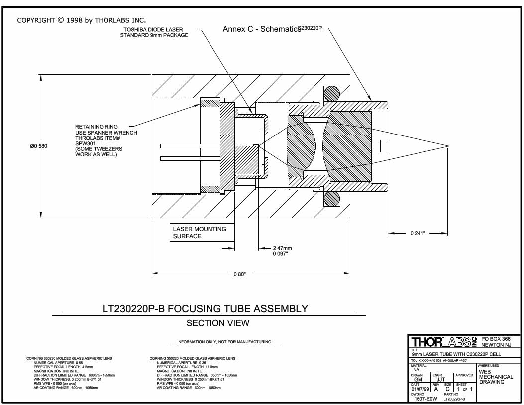
At the beginning, the LT230220P-B (an optical Laser Package with a focusing

tube with C230220P-B optic) pair was used to impinge light to the target. Here, we have

been confronted with diffraction problems caused by the system optical aperture. So, the

focusing tube was replaced by a collimation tube, the LT220P-B. Both assemblies are

schematized in annex C.

Further, experiments were made using multimode and single-mode fibers as light

conveyors. Like Wang [9], we concluded that the self-mixing effect does not appear to

depend on whether the fiber used to couple the source to the target is single-mode or

multimode.

The use of prototype 1 was then abandoned and a new prototype, prototype 2,

incorporating a pigtailed laser diode was put in use. The pigtail solution provides good

coupling efficiency between the laser diode and the fiber, and as an additional advantage

of this design, should the diode ever fail, it could be easily replaced while reusing the rest

of the optics.

Two important experimental studies of self-mixing interferometry were

performed before trying the biomedical measurements. Bench Test I is about the test of

the self-mixing effect using a loudspeaker, and Bench Test II is about the same using a

moving strip.

5.2.2. Interface system

5.2.2.1. Circuit

The printed circuits were elaborated with the help of OrCAD®. This tool offers

PCB designers, the power and flexibility to create and share PCB building data.

OrCAD® layout delivers all the capabilities designers need, from netlist, to route and

place. The PCB design of the LDF work is illustrated in annex D.

The printed circuit has double face, has plated through holes and has a mask

solder.


30

The electrical and electronic circuit components were then mounted and the

results were already shown in figure 17.

The circuit has two essential constituents, the Power Supply and the Laser Driver.

The Power Supply is +/-5V because these values are compatible with the specifications

of the components, particularly those of the OpAmps. The Laser Driver is constituted by

5 main blocs, as it can be seen in annex E. They are:

• Dual Polarity Current Source

Figure 18: Schematic of the dual polarity current source.

The scheme depicted in figure 18 is due, essentially, to provide dual polarity

current to activate the laser diode. The components that must be noted are:

- The darlington Transistor (Q1). It gives a high current gain to the circuit.

Because it works as a dual polarity current source, it can be a PNP if it works as a

current source (see figure 18) or a NPN if it works as a current sink. In this last

case the switches SW1 and SW2 must be set, differently.

- The trimmer (R40), a variable resistor component allowing making fine

adjustments to its resistance, to control the current;

- MAX320/SO (U18), an electric switch which allows lighting the laser in a

progressive way. If it is in closed, the Zener diode (D1) has no current and the

laser turns off, otherwise the Zener conducts and the laser turns on.


31

• The Transconductance Amplifier

• The Transconductance Amplifier/ Voltage Follower

The block of the figure 20 corresponds to a voltage follower, however, without

R34 it becomes to a transconductance amplifier.

• The Audible Monitoring

Iin Vout

Vout

Figure 19: Schematic of the transconductance amplifier used in laser driver circuit.

Figure 20: Schematic of the voltage follower. If we take off R34 it becomes a transconductance amplifier.


32

• The DC-DC Converter

Figure 22: Schematic of the DC-DC Converter.

5.2.2.2. USB-6009

Figure 23: NI USB-6009. (Adapted from [23])

Figure 21: Schematic of the audible monitoring.


33

The National Instrument USB-6009 multifunction data acquisition (DAQ) module

showed in figure 23 provides reliable data acquisition at low price. With plug-and-play

USB connectivity, this module is simple enough for quick measurements but versatile

enough for more complex measurement applications. The NI USB-6009 uses NI-

DAQmx high-performance and multithreaded driver software for interactive

configuration. All NI data acquisition devices shipped with NI-DAQmx also includes the

VI Logger Lite, a configuration-based data logging software package. The USB-6009 has

removable screw terminals for easy signal connectivity. It is ideal for a number of

applications such as:

Data logging – Log environmental or voltage data quickly and easily;

Academic lab use.

The specifications of the Low-Cost Multifunction DAQ for USB are described in

annex F. Some of them are:

• 8 analogue inputs (14-bit, 48 kS/s);

• 2 analogue outputs (12-bit, 150 S/s); 12 digital I/O; 32 bit counter;

• Bus-powered for high mobility; built-in signal connectivity;

• Compatible with LabVIEW, LabWindows/CVI, and Measurement Studio for

Visual Studio.NET.

5.2.3. Data acquisition and signal processing

The data acquisition and signal processing are done with a PC. As mentioned

before, the board interfaces easily with Matlab. We choose Matlab to be equipped with

the Data Acquisition Toolbox 2.9 that provides a set of tools for analogue input, analogue

output and digital I/O from a variety of PC-compatible data acquisition hardware. The

toolbox supports a lot of popular hardware devices, but we are interested in National

Instruments boards that use Traditional NI-DAQ or NI-DAQmx driver software [24].


34

Start

Definition of Variables

File choice for what we intend to read

Signal Visualization

Signal Filtering

Filtered Signal Visualization

FFT Visualization

Save data to EXCEL file

Spectrogramme Visualization

PDF Visualization

End

Specifically for the present application, a Matlab program was created to study

LDF data acquisition. This program is in annex G. The flowchart in figure 24

demonstrates how the Matlab programmer provides visualization of the LDF signal.

Figure 24: Flowchart of the Matlab programmer.


35

The Doppler signal analysis is based on Fast Fourier Transform (FFT) calculation.

This is done because in the time domain it is very difficult to calculate fringes due to

fluctuations.

It is possible to relate the Probability Density Function (PDF) with the Doppler

frequency spectrum. This subject will be discussed, in more detail, in section 6.

5.3. Bench Test I

Figure 25: Image of the experimental arrangement I for LDF detection.

The experimental arrangement related to the loudspeaker setup is showed in

figure 25.

A Pigtailed laser diode (LPM-660-SMA) with a wavelength of 660 nm, with an

output optical power 22,5mW and a multimode optic fiber were used in the experiment.

The light from the pigtail was emitted from the fiber and reflected back into the laser

cavity via the same fiber. A reflective surface attached to a loudspeaker cone driven by a

Loudspeaker

Reflective Surface

Micrometer

Laser Diode Fiber Pigtail (λ=660nm)

Electronic Box


36

signal generator was used as a target, to provide phase variations of the external optical

feedback.

The HL6501MG diode laser package incorporates a photodiode (PD)

accommodated in the rear facet to monitor the laser power. This characteristic of the

device is particularly well suited to observing the self-mixing interference, and it

provides a convenient internal detector. The end of the fiber was fixed at 45 degrees

angle, near to the reflective surface. The distance from the fiber end to the reflective

surface was about 2 mm. A PC with Matlab data acquisition (see section 5.2.3) was used

to record the output signal.

A total of 40000 samples were recorded for each period over a time of nearly 5

seconds. The voltage amplitude feeding the loudspeaker’s membrane was constant, with

the value of 10 mV. The purpose was to vary the modulated frequency and observes the

changes in the Doppler spectra.

5.4. Bench Test II

The experimental arrangement related to the moving strip setup is showed in

figure 26.

In this bench test, the light from the Pigtailed laser diode (LPS-1310-FC, single-

mode fiber) with a wavelength of 1310 nm and with an output optical power of 2,5 mW,

was emitted from the fiber and reflected back into the laser cavity via the same fiber. As a

reflective surface it was used a white paper strip, because it was highly scattering such as

the human skin. The target was moved at a certain velocity. The end of the fiber was

fixed at a 45 degrees angle, near to the moving strip, and the distance from the fiber end

to the moving strip was about 1 mm, as showed in figure 26. Then, the output signal was

recorded with a PC with the Matlab data acquisition tool, mentioned before.


37

A total of 40000 samples were recorded for each period over a time of nearly 5

seconds. The strip movement is repeated for increasing velocity regimes. The purpose

was to vary the velocity and observe the changes in the Doppler spectra.

Figure 26: Image of the experimental arrangement II for LDF detection.

υ

Moving Strip

Mechanical Support

Electronic Box

Laser Diode Fiber Pigtail

Laser Diode Fiber Pigtail (λ=1310nm)

Laser Doppler Flowmetry CHAPTER 6 – RESULTS

38

6. Results

In this chapter, a dimensioning of theoretical background will be made. The

results of the experiments on the self-mixing arrangement for LDF with a loudspeaker

will be presented. Suggestions for future work will also be drawn.

6.1. Dimensioning

In this section the order of magnitude of the frequency beating values will be

estimated for the self-mixing geometry that we are studying and has been reviewed in

sections 2.8. and 4.

As was referred in section 2.3, the Doppler effect is based in a frequency shift, ωd,

expressed by the equation (1). Recalling that angles α and θ were defined as

we will now estimate ωd for this geometry based on figure 27 where and .

[ ]si KKrr

,=α [ ]qrr,νθ =

Figure 27: The loudspeaker arrangement.

Loudspeaker

FIBER

ikr

skr

ikr

skr

qr

qrvr

α θ


39

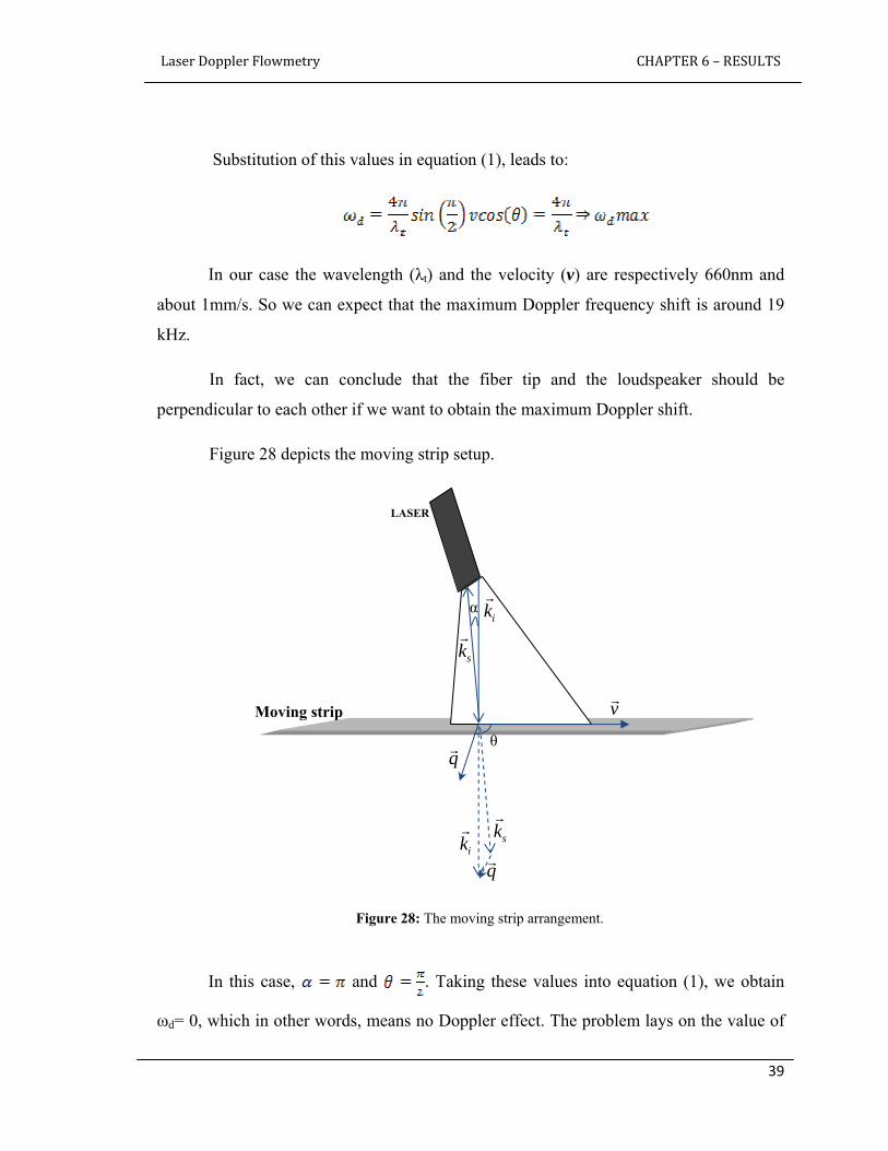
Substitution of this values in equation (1), leads to:

In our case the wavelength (λt) and the velocity (v) are respectively 660nm and

about 1mm/s. So we can expect that the maximum Doppler frequency shift is around 19

kHz.

In fact, we can conclude that the fiber tip and the loudspeaker should be

perpendicular to each other if we want to obtain the maximum Doppler shift.

Figure 28 depicts the moving strip setup.

In this case, and . Taking these values into equation (1), we obtain

ωd= 0, which in other words, means no Doppler effect. The problem lays on the value of

Figure 28: The moving strip arrangement.

vrMoving strip

LASER

ikr

skr

ikr

skr

qr

qr

α

θ


40

θ and the solution is not to keep the laser perpendicular to the surface of the moving strip

but rather to tilted as much as possible, so that θ gets close to zero.

6.2. Functional Tests

6.2.1. Bench Test I

A typical output obtained at the bench test I is shown in figure 29.

The lower trace in figure 29 is the signal applied to achieve the periodic target

movement, and the resultant intensity modulation (upper trace) is the self-mixing

interference signal observed. The extremes of the displacement curve correspond to the

zero-velocity instants. During the positive velocity, or when approaching, each of the

sawtooth-like waveforms rises rapidly and falls slowly, while during the negative

velocity vice versa.

The spectra for the time series depicted in figure 29 are shown in figure 30. Five

different modulated frequencies are shown.

Figure 29: Typical signals observed in self-mixing – lower trace, loudspeaker membrane movement – upper trace, self-mixing signal from PD.


41

Figure 30: Frequency Beating Spectra.

We will now use these results to calculate the membrane amplitude.

If the membrane position (x) is given by , the velocity will be:

Taking the modulated frequency of 50 Hz (orange line), in figure 29 where a

maximum frequency of 15 kHz is readable, and for the values used in the experiment:

Taking the modulated frequency of 30 Hz where the maximum frequency of

is readable, the amplitude is approximately 12 µm.

These amplitude values are reasonable in accordance with typical data from

loudspeaker datasheets.

0 1.8 3.6 5.4 7.2 9 10.8 12.6 14.4 16.2


42

We can also conclude that the results of the graphic are in agreement with

equation (1): the Doppler frequency shift (ωd) increases when the modulated frequency

(w) increases.

It seems possible to relate the frequency beating spectra with the PDF of the raw

data. This is suggested by curves of figure 29 where the typical saddle-shaped curve

shows up.

As a hint, we do not close the possibility of the exploration of the connection

between the beating frequency spectrum and the PDF, for standard cases.

6.3. Another Bench Tests

An experiment in which a flow regime of known characteristics is established was

setup to test the LDF instrumentation. The target was a fluid with a diluted scattered

(talcum powder) flowing in a transparent tube. The idea was to approximate the target as

much as possible to the blood flow in terms of flow velocity. So, we developed a

hydraulic model that is schematically drawn in figure 31:

Figure 31: Hydraulic Model. The solution enters to the tube and flows through it.

Tube

LaserWater

and Talc

Bottle


43

The talc was chosen because it is highly scattering like the human skin. This

solution was in a recipient and was then pumped through a plastic tube (inner diameter 3

mm) which was fixed in a breadboard. The different speeds of pumping of the water/talc

solution were achieved by gravitation and a progressive tap. The laser Doppler fiber

pigtail was positioned almost perpendicularly to the surface of the tube.

Unfortunately, there was no time to perform consistent measurements.

Another idea suggested as future work uses a peristaltic pump to obtain a pulsatile

regime of similar characteristics to the human dynamic system.

Laser Doppler Flowmetry CHAPTER 7 – CONCLUSIONS AND FUTURE WORK

44

7. Conclusions and Future Work

This report has reviewed the main theoretical background that underlies beneath

Laser Doppler technique, as well as aspects of the detection geometries and implications

derived from using optical fiber for light transportation.

The state of the art of commercially available instruments for research and clinical

use has also been reviewed with a simple conclusion that equipments are very expensive

and only two major European manufacturers are currently in the marketplace with

interesting solutions.

Especially developed experimental set-ups have been implemented with the

purpose of studying the properties of typical LDF signals. These experiments have made

clear some limitations of the data acquisition hardware as well as some signal processing

algorithms.

As for the data acquisition hardware, it became very clear that the NI6009

sampling rate (48 ksps total, for all channels) is not enough in many practical situations.

The NI6210, with its 250 ksps, will be a better option in future developments, although it

comes at a 3 times higher price.

Concerning the signal processing algorithms, it also became evident that the

classic Fourier transform (or its simplified relative, the FFT) does not provide adequate

information in the context of this application. In fact, for the long time intervals, that are

common in LDF, the Continuous Wavelet Transform (CWT) is generally recognized as a

superior analysis tool since it allows spectral analysis without loss of time information.

Experiments on the self-mixing arrangement for LDF with the loudspeaker have

proved to be very effective and insightful. Data collected with this system is shown and

some speculation concerning its interpretation is developed.

Laser Doppler Flowmetry CHAPTER 7 – CONCLUSIONS AND FUTURE WORK

45

Data collected in this experiment is also used to determine the amplitude of the

loudspeaker movement when it is driven by a sinusoidal waveform. This experiment also

demonstrates the adequacy of the instrument as a laser vibrometer.

Experiments with a different scattering system – a unidirectionally moving strip

of paper – were not completed, and were consequently misleading, due to lack of time.

Laser Doppler Flowmetry CHAPTER 8 – REFERENCES

46

8. References

[1] Jones Deric P, “Medical Electro-optics: measurements in the human microcirculation”,

1987, Phys. Technol., 18, 79-85

[2] Anderson, R.R. and Parrish, “Optical Properties of Human Skin”, 1987 (New York)

[3] Tuchin V, “Tissue Optics: Light Scattering Methods and Instruments for Medical

Diagnosis”, 2000

[4] Fredriksson I, Fors C and Johansson J, “Laser Doppler Flowmetry – a Theoretical

Framework”, 2007, Linköping University, Department of Biomedical Engineering

[5] http://en.wikipedia.org/

[6] Briers J D, “Laser Doppler, speckle and related techniques for blood perfusion mapping

and imaging”, 2001, Physiol. Meas., 22, R35-R66

[7] Forrester K R, Tutil J, Leonard C, Stewart C, Bray R C, “A Laser Speckle Imaging

Technique for Measuring Tissue Perfusion”, 2004, iEEE Transactions on Biomedical

Engineering, Vol. 51 No. 11, pages 2074-2084

[8] Smedley G, Yip Kay-Pong, Wagner A, Dubovitsky S, Marsh D J, “A laser Doppler

instrument for in vivo measurements of blood flow in single renal arterioles”, 1993, iEEE

Transactions on Biomedical Engineering, Vol. 40 No. 3, pages 290-297

[9] Wnag W M, Boyle J O, Grattan K T V, Palmer A W, “Self-mixing interference in a diode

laser: experimental observations and theoretical analysis”, 1993, Applied Optics, vol.32

No.9, 1551-1558

[10] Humeau A, Köitka A, Abraham P, Saumet J, L’Huillier Jean-Pierre, “Spectral components

of laser Doppler Flowmetry signals recorded in healthy and type 1 diabetic subjects at rest

and during a local and progressive cutaneous pressure application: scalogram analyses”,

2004, Phys. Med. Biol., 49, 3957-3970


47

[11] Serov A, Steunacher B and Lasser T, “Full-field laser Doppler perfusion imaging and

monitoring with an intelligent CMOS camera”, 2005, Optics Express, vol. 13 No. 17, 6416-

6428

[12] Serov A and Theo L, “Blood flow imaging is enhanced using new detector technology”,

Laboratoire d’Optique Biomedicale, École Polytecnique Fédérale de Laussanne

[13] Sinohara S, Mochizuki A, Yoshida H and Sumi M, 1986, Appl.Opt., 25, 1417–9

[14] Slot M, KoelinkM H, Scholten F G, de Mul F F M, Weijers A L, Greve J, Graff R, Dassel

A C M, Aarnoudse J G and Tuynman F H B, 1992, Med. Biol. Eng.Comput., 30, 441–6

[15] de Mul F F M, KoelinkM H, Weijers A L, Greve J, Aarnoudse J G, Graff R and Dassel A C

M, 1992, Appl. Opt,. 27, 20

[16] Jukka Hast, “Self-mixing interferometry and its applications in non invasive pulse

detection”

[17] Özdemir S K, Shinohara S, Takamiya S and Yoshida H, “Noninvasive blood flow

measurement using speckle signals from a self-mixing laser diode: in vitro and in vivo

experiments”, 2000, Opt. Eng, 39(9), 2574-2580

[18] Petermann K, “ Laser Diode Modulation and Noise”, 1988, Kluwer Academic, Dordrecht,

Netherlands

[19] Meigas K, Hinrikus H, Kattai R, Lass J, “Self-mixing in a diode laser as a method of

cardiovascular diagnostics”, January 2003, Journal of Biomedical Optics 8(1), 152-160

[20] http//bmo.tnw.utwente.nl/vinay/principle_of_laser_doppler_flowm

[21] http://www.discovtech.com/PAGE5.htm

[22] http://www.perimed.se/p_Products/periflux.asp

[23] Nilsson G E, Salerud E G, Strömberg NOT, Wårdell K, “Laser Doppler Perfusion

Monitoring and Imaging”, In: Vo-Dinh T, editor: Biomedical photonics handbook, Boca

Raton, Florida:CRC Press, 2003, p. 15:1-24

[24] http://sine.ni.com/nips/cds/view/p/lang/en/nid/14605


48

[25] http://www.mathworks.com/index.html?ref=pt

[26] Öberg P Å, “Optical Sensors in Medical Care”, Sensors Update 3

Annex A - Simulation of the beating frequency phenomenon

%Project: 'Evaluation of Hemodynamic Parameters: LDF' %Observation of the frequency beating phenomenon - July 2007 npts=50000; %number of points na=34; %number of periods ampl=1; %amplitude x=seno(npts,na,ampl); % Creates a sino function npts=50000; na=37; ampl=1; y=seno(npts,na,ampl); for k=1:npts; soma(k)=x(k)+y(k); %Sum of two waves end for t=1:npts; i(t)=soma(t)*soma(t); %Calculates the irradiance end figure(1); subplot(4,1,1); plot(x); title('F1'); subplot(4,1,2); plot(y); title('F2'); subplot(4,1,3); plot(soma); title('Beating F1+F2'); subplot(4,1,4); plot(i); title('Irradiance');

Annex B - Specifications table of DTI OxyLab LDF and OxyFlo.

Adapted from [22]

9mm MOUNTING

5 4 3 2 1

LT220P-B

MATERIAL:

PART NO.

TOLERANCES

PROPRIETARY AND CONFIDENTIAL N/A

LT220P-B COLLUMATION

ONE PLACE DECIMAL:

FLANGE OF THE LASER

THE INFORMATION CONTAINED IN THIS

DIMENSIONS ARE IN MILLIMETERS

DRAWING IS THE SOLE PROPERTY OF

0.2LINEAR TOLERANCES:

30'

DRAWN

ENG APPR.

MFG APPR.

NAME

TITLE:

SIZEA

REV.

SCALE: 3:1 SHEET 1 OF 1

0895-E01

ANGULAR: 0.04 TWO PLACE DECIMAL:

THORLABS, INC. IS PROHIBITED.

UNLESS OTHERWISE SPECIFIED:

DWG. NO.

REV. # DESCRIPTION: NAME/DATE:

BAG

TO

TO

10/23/2006

DATE

10/23/2006

10/23/2006

THORLABS INC.

THE WRITTEN PERMISSION OF

NEWTON NJ

SPECIFICATIONS:

PO BOX 366

IN PART OR AS A WHOLE WITHOUT

THORLABS, INC. ANY REPRODUCTION

THE LT220P-B WAS DESIGNED USING THE TOSHIBA STANDARD1.9mm LASER DIODE PACKAGE. THE PRINCIPLE PLANE OF THEC220TM (f= 11mm) IS NOMINALLY 13.47mm FROM THE LASERMOUNTING SURFACE

2. THE C220TME LENS CELL HAS 1mm OF ADJUSTMENT RANGE FROM THE POSITION SHOWN IN THE ASSEMBLY DRAWING

3. THE LT220A DESIGN REQUIRES THE EMITTING SURFACE OF THELASER TO BE BETWEEN 1.7mm TO 3.2mm FROM THE

THIS DRAWING IS FOR INFORMATION ONLYNOT INTENDED FOR MANUFACTURING

LT220P-B COLLIMATION TUBE TYPICAL ASSEMBLYSECTION VIEW

2:1 SCALE

RMS WFE <0.050 (ON AXIS)AR COATING RANGE: 600nm-1050nmGLASS (CORNING): ECO550

LASER DIODE PACKAGESTANDARD 9mm TOSHIBASPW301 COMPATABLE

MOUNTED CORNING 352220 MOLDED GLASS ASPHERIC

SPECIFICATIONS:NUMERICAL APERTURE: 0.25EFFECTIVE FOCAL LENGTH: 11.0 mmMAGNIFICATION: INFINITEDIFFRACTION LIMITED RANGE: 350 nm-1550nmWINDOW THICKNESS: 0.25mm

RETAINING RING SPANNER WRENCH

IDENTIFICATION GROOVE

14.70.580

25.41.000

Annex C - Schematics

Annex C - Schematics

Annex D - PCB design

5

5

4

4

3

3

2

2

1

1

D D

C C

B B

A A

VDD

VEE

VDDVCC

VCC

VDD

VCC

VCC

VCC

VDD

VCC

VDD

VCC

VDD

VDDVDD

VCC

VCC

VCC

VCC

DAC-HV control

APD

Title

Size Document Number Rev

Date: Sheet of

<Doc> 2

Laser Driver / Amp

A3

3 3Thursday, November 30, 2006

Title


Date: Sheet of

<Doc> 2

Laser Driver / Amp

A3


Title


Date: Sheet of

<Doc> 2

Laser Driver / Amp

A3


Laser Driver

-5 V

Laser Diode

DAC (opt)

Thermometer(AD590 or LM35)

R24R24

R35R35

C28C28

R2R2

SW2SW2

R34R34

-

+

U1B

-

+

U1B

5

67

411

C11C11

R25R25

+ C38+ C38

SW3SW3

D1D1

-

+

U1C

-

+

U1C

10

98

411

R27R27

R38R38

J5J5

123456

-

+

U1D

-

+

U1D

12

1314

411

C1C1

R39R39

U5

IL1205

U5

IL1205

Vin2

Zero 3

Vout 4

Gnd1

R60R60

-

+

U1A

-

+

U1A

3

21

411

R37R37

C40C40

U19

TDA7052

U19

TDA7052

a 2

b 3

o+5

o-8

v+1

gnd

6

C39C39

R1R1

SW1SW1

C12C12

C2C2

R36R36

C29C29

-

+

U20A

TL072/SO

-

+

U20A

TL072/SO

3

21

84

Q1Q1

R28R28

J6J6

12

SW5SW5

R26R26

LS1

SPEAKER

LS1

SPEAKER

C3C3

J1

CON3

J1

CON3

123

U18

MAX320/SO

U18

MAX320/SO

NO1 1NO2 5

V+8V-4

COM12COM26

IN17IN23

C30C30

R40R40

+

C27

+

C27

Annex E - Schematic of the Laser Driver

Ana

Text Box

Annex E - Schematic of the Laser Driver

SpecificationsTypical at 25 °C unless otherwise noted.

Analog InputAbsolute accuracy, single-ended

Absolute accuracy at full scale, differential1

Number of channels............................ 8 single-ended/4 differentialType of ADC ........................................ Successive approximation

ADC resolution (bits)

Maximum sampling rate (system dependent)

Input range, single-ended................... ±10 VInput range, differential...................... ±20, ±10, ±5, ±4, ±2.5, ±2,

±1.25, ±1 VMaximum working voltage ................. ±10 VOvervoltage protection ....................... ±35 VFIFO buffer size ................................... 512 BTiming resolution ................................ 41.67 ns (24 MHz timebase)Timing accuracy .................................. 100 ppm of actual sample rateInput impedance ................................. 144 kTrigger source...................................... Software or external digital triggerSystem noise....................................... 0.3 LSBrms (±10 V range)

Analog OutputAbsolute accuracy (no load) ............... 7 mV typical, 36.4 mV maximum

at full scaleNumber of channels............................ 2Type of DAC ........................................ Successive approximationDAC resolution .................................... 12 bitsMaximum update rate ........................ 150 Hz, software-timed

1Input voltages may not exceed the working voltage range.

Output range ....................................... 0 to +5 VOutput impedance............................... 50 ΩOutput current drive............................ 5 mAPower-on state.................................... 0 VSlew rate............................................. 1 V/µsShort-circuit current ............................ 50 mA

Digital I/ONumber of channels............................ 12 total

8 (P0.<0..7>)4 (P1.<0..3>)

Direction control ................................. Each channel individually programmable as input or output

Output driver typeUSB-6008........................................ Open-drainUSB-6009........................................ Each channel individually

programmable as push-pull oropen-drain

Compatibility ....................................... CMOS, TTL, LVTTLInternal pull-up resistor ...................... 4.7 kΩ to +5 VPower-on state.................................... Input (high impedance)Absolute maximum voltage range...... -0.5 to +5.8 V

Digital logic levels

CounterNumber of counters ............................ 1Resolution ........................................... 32 bitsCounter measurements....................... Edge counting (falling edge)Pull-up resistor .................................... 4.7 kΩ to 5 VMaximum input frequency.................. 5 MHzMinimum high pulse width................. 100 nsMinimum low pulse width.................. 100 nsInput high voltage ............................... 2.0 VInput low voltage ................................ 0.8 V

Power available at I/O connector

+5 V output (200 mA maximum) ......... +5 V typical+4.85 V minimum

+2.5 V output (1 mA maximum) .......... +2.5 V typical +2.5 V output accuracy ....................... 0.25% maxVoltage reference temperature drift... 50 ppm/°C max

Low-Cost Multifunction DAQ for USB

3

BUY ONLINE at ni.com or CALL (800) 813 3693 (U.S.)

Module Differential Single-EndedUSB-6008 12 11USB-6009 14 13

Range Typical at 25 ˚C (mV) Maximum (0 to 55 ˚C) (mV)±10 14.7 138

Module Maximum Sampling Rate (kS/s)USB-6008 10USB-6009 48

Level Min Max UnitsInput low voltage -0.3 0.8 VInput high voltage 2.0 5.8 VInput leakage current – 50 µAOutput low voltage (I = 8.5 mA) – 0.8 VOutput high voltage (push-pull, I = -8.5 mA) 2.0 3.5 VOutput high voltage (open-drain, I = -0.6 mA, nominal) 2.0 5.0 VOutput high voltage (open-drain, I = -8.5 mA, with external pull-up resistor) 2.0 – V

Range Typical at 25 ˚C (mV) Maximum (0 to 55 ˚C) (mV)±20 14.7 138±10 7.73 84.8±5 4.28 58.4±4 3.59 53.1±2.5 2.56 45.1±2 2.21 42.5±1.25 1.70 38.9±1 1.53 37.5

Annex F - Specifications of the Low-Cost Multifunction DAQ for USB

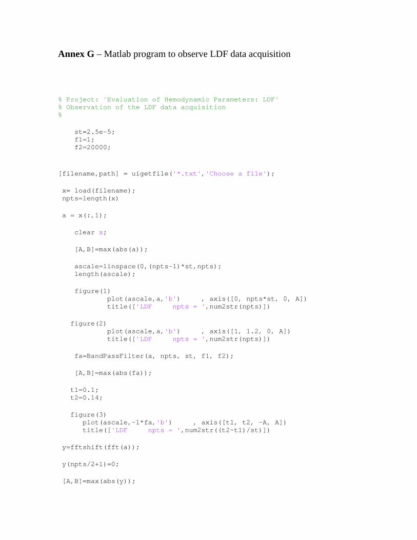
Annex G – Matlab program to observe LDF data acquisition

% Project: 'Evaluation of Hemodynamic Parameters: LDF' % Observation of the LDF data acquisition % st=2.5e-5; f1=1; f2=20000; [filename,path] = uigetfile('*.txt','Choose a file'); x= load(filename); npts=length(x) a = x(:,1); clear x; [A,B]=max(abs(a)); ascale=linspace(0,(npts-1)*st,npts); length(ascale); figure(1) plot(ascale,a,'b') , axis([0, npts*st, 0, A]) title(['LDF npts = ',num2str(npts)]) figure(2) plot(ascale,a,'b') , axis([1, 1.2, 0, A]) title(['LDF npts = ',num2str(npts)]) fa=BandPassFilter(a, npts, st, f1, f2); [A,B]=max(abs(fa)); t1=0.1; t2=0.14; figure(3) plot(ascale,-1*fa,'b') , axis([t1, t2, -A, A]) title(['LDF npts = ',num2str((t2-t1)/st)]) y=fftshift(fft(a)); y(npts/2+1)=0; [A,B]=max(abs(y));

fscale=linspace(-0.5/st, 0.5/st, npts); figure(4) plot(fscale, abs(y)) , axis([0, 0.5/st, 0, A ]) title(['FFT' ]) m=20; nnn=round(npts/2/m); for w=1:nnn sum=0; for k=1:10 sum=sum+abs(y(k+w*m)); end fg(nnn-w+1)=sum; end % n2=length(fg); % % f2scale=linspace(0, 0.5/st, n2); % figure(5) % plot(f2scale,fg) % s=fg.'; % sc=f2scale.'; % save('res_50_10.txt', 's', '-ASCII'); % save('res_50_10_sc.txt','sc', '-ASCII'); % clear all

laser doppler flowmetry - estudo geral · among the few diagnostic techniques available, laser...

Documents