arX

iv:m

ath/

0610

715v

5 [

mat

h.D

S] 1

7 Se

p 20

11 Lattice Point Asymptotics and Volume Growth on

Teichmuller Space.

Jayadev Athreya∗, Alexander Bufetov†, Alex Eskin‡and Maryam Mirzakhani§

September 20, 2011

Abstract

We apply some of the ideas of the Ph.D. Thesis of G. A. Margulis [Mar70] to Teichmullerspace. Let X be a point in Teichmuller space, and let BR(X) be the ball of radius R centeredat X (with distances measured in the Teichmuller metric). We obtain asymptotic formulas asR tends to infinity for the volume of BR(X), and also for the cardinality of the intersection ofBR(X) with an orbit of the mapping class group.

1 Introduction.

Much of the study of the geometry and dynamics on Teichmuller and moduli spaces is inspired byanalogies with negatively curved spaces. Two classical problems in the negative curvature setting arethe questions of lattice point counting and volume growth entropy. Let M be a compact negativelycurved Riemannian manifold, and M its universal cover. Π = π1(M) acts on M by isometries. Let

mBM denote the Bowen-Margulis measure on M . Given X,Y ∈ M , R > 0, let BR(X) ⊂ M be the

ball of radius R centered at X. Let p : M →M be the natural projection.In his Ph.D. thesis G. A. Margulis [Mar70] showed:

Theorem 1.1 There is a function c :M ×M → R+ so that for every X,Y ∈ M ,

|Π · Y ∩BR(X)| ∼ c(p(X), p(Y ))ehR (1.1)

mBM (BR(X)) ∼(∫

M

c(p(X), z)dmBM (z)

)ehR (1.2)

where h > 0 is the topological entropy of the geodesic flow. Here and below, the notation A ∼ Bmeans that A/B → 1 as R→ ∞.

∗partially supported by NSF grants DMS 0603636, DMS 0244542 and DMS 1069153†A.I.B. is an Alfred P. Sloan Research Fellow. He is supported in part by Grant MK-4893.2010.1 of the President of

the Russian Federation, by the Programme on Mathematical Control Theory of the Presidium of the Russian Academyof Sciences, by the Programme 2.1.1/5328 of the Russian Ministry of Education and Research, by the Edgar OdellLovett Fund at Rice University, by the NSF under grant DMS 0604386, and by the RFBR-CNRS grant 10-01-93115.

‡partially supported by NSF grants DMS 0244542, DMS 0604251 and DMS 0905912§partially supported by the Clay foundation and by NSF grant DMS 0804136.

1

In this paper, we apply some of the ideas of Margulis from [Mar70] to the problems of countinglattice points and understanding volume growth entropy in Teichmuller space. Our main results(Theorems 1.2 and 1.3) are analogues of Theorem 1.1 for Teichmuller space, and the fact thatthe Bowen-Margulis measure coincides with the Lebesgue measure (see §2.2). In the rest of thisintroduction we give the required background and definitions of Teichmuller space and quadraticdifferentials, and state our main results.

1.1 Teichmuller space and quadratic differentials.

We briefly recall some defintions. For a more detailed introduction, see, e.g., [FaMa]. Let g ≥ 2,and let Σg be a compact topological surface of genus g. Let Mg and Tg denote the moduli spaceand the Teichmuller space of compact Riemann surfaces of genus g.

That is, Tg is the space of equivalence classes of pairs (X, f) where X is a compact genus gRiemann surface and f : Σg → X is a diffeomorphism (known as a marking). The equivalencerelation is given by (X, f) ≈ (Y, h) if there is a biholomorphism φ : X → Y so that h−1 φ f isisotopic to the identity.

Let Γ be the mapping class group of Σg, given by isotopy classes of orientation preservingdiffeomorphisms of Σg. That is, Γ = Diff+(Σg)/Diff+

0 (Σg). Γ acts on Tg by changing the marking,and we have Mg = Tg/Γ.

Tg carries a natural Finsler metric invariant under Γ, known as the Teichmuller metric. It isgiven by measuring the quasi-conformal dilatation between surfaces, see, e.g. [FaMa]. The cotangentspace of Tg at a point X can be identified with the vector space Q(X) of holomorphic quadraticdifferentials on X. Recall that given X ∈ Tg, a quadratic differential q ∈ Q(X) is a tensor locallygiven by φ(z)dz2 where φ is holomorphic with respect to the complex structure given by X . Thenthe space QTg = (q,X) | X ∈ Tg, q ∈ Q(X) is the cotangent space of Tg. In this setting, theTeichmuller metric corresponds to the norm

‖ q ‖T =∫

X

|φ(z)| |dz|2

on QTg.Let Q1Mg (resp. Q1Tg) denote the bundle of unit-norm holomorphic quadratic differentials on

Mg (resp. Tg). We have Q1Mg = Q1Tg/Γ.The space Q1Tg carries a natural smooth measure µ, preserved by the action of Γ and such that

µ(Q1Mg) <∞ ([Mas82], [Ve82]). We will fix a normalization for µ in §2.2.We have a natural projection

π : Q1Tg → Tgand we set m = π∗µ.

1.2 Statement of results.

Let X,Y ∈ Tg be arbitrary points, and let BR(X) be the ball of radius R in the Teichmuller spacein the Teichmuller metric, centered at the point X .

Our main results are the following two theorems:

2

Theorem 1.2 (Lattice Point Asymptotics) As R→ ∞,

|Γ · Y ∩BR(X)| ∼ 1

hm(Mg)Λ(X)Λ(Y )ehR,

where h = 6g − 6 is the entropy of the Teichmuller geodesic flow with respect to Lebesgue measure(see [Ve86]), and Λ is a bounded function called the Hubbard-Masur function, which we define in§2.3.

Theorem 1.3 (Volume Asymptotics) As R → ∞,

m(BR(X)) ∼ 1

hm(Mg)ehRΛ(X) ·

∫

Mg

Λ(Y ) dm(Y ).

We also prove versions of the above theorems in “sectors”, see Theorem 2.9, Theorem 2.10 andTheorem 5.2 below.

Acknowledgments. The authors are grateful to Giovanni Forni, Vadim Kaimanovich, Yair Minskyand Kasra Rafi for useful discussions, and especially to Howard Masur for his help with all partsof the paper, in particular the appendix. We are also grateful to the Institute for Advanced Study,IHES and MSRI for their support.

1.3 Organization of the paper.

This paper is organized as follows: In §2, we describe the main ingredients in the proofs of ourmain theorems. We construct foliations and measures satisfying the Margulis property of uniformexpansion in §2.2. We define the Hubbard-Masur function Λ and describe its basic properties andrelation to counting multicurves in §2.3. In §2.4 we state a crucial lemma, Proposition 2.5, onmeasure in polar coordinates. We postpone the proof to §3.2. In §2.5 we show how to use mixing toobtain equidistribution results, and apply them to the counting problem in §2.6. In §3 we recall thedefinition of the Hodge norm for abelian differentials (§3.1), and extend and modify it to quadraticdifferentials (§3.3). We use this to define a distance along leaves of the stable and unstable foliationsfor the Teichmuller geodesic flow, and compare it to other distances on Tg in §3.5. We prove anon-expansion result for this distance, Theorem 3.15, in §3.6. In §4, we use the results of §3 to provethe key estimates Theorem 2.6 and Theorem 2.7 from §2.5. Finally, in §5, we prove our volumeasymptotics result, Theorem 1.3, and relate it to counting multicurves.

2 Outline of Proof.

2.1 Notation and background.

Teichmuller geodesic flow. We recall that when g > 1, the Teichmuller metric is not Riemannian.However, geodesics in this metric are well understood. A quadratic differential q ∈ QTg with zerosat x1, . . . , xk is determined by an atlas of charts φi mapping open subsets of Σg − x1, . . . , xkto R2 such that the change of coordinates are of the form v → ±v + c. Therefore the group SL2(R)acts naturally on QMg by acting on the corresponding atlas; given A ∈ SL2(R), A · q ∈ QMg isdetermined by the new atlas Aφi.

3

Let gt =

[et 00 e−t

]. The action of the diagonal subgroup gt | t ∈ R is the Teichmuller geodesic

flow for the Teichmuller metric (see [FaMa]).

Warning. In our normalization for the Teichmuller metric, the Teichmuller distance between π(gtq)and π(q) is t. This normalization (and thus our value for the entropy h) differs by a factor of 2 fromthat of e.g. [Ve86]. Our normalization is chosen in such a way that the top Lyapunov exponent ofthe Kontsevich-Zorich cocycle is equal to one. In this case the top Lyapunov exponent of the flowis equal to two. For a detailed discussion of the connection between the Lyapunov exponents of theTeichmuller geodesic flow and the Kontsevich-Zorich cocycle, see, e.g., [Fo02], where the same speednormalization is used for the Teichmuller geodesic flow as in our paper.

We have [Ve82], [Mas82]:

Theorem 2.1 (Veech, Masur) The space Q1Mg carries a unique up to normalization measure µin the Lebesgue measure class such that:

• µ(Q1Mg) <∞.

• the action of SL2(R) is volume preserving and ergodic;

• the Teichmuller geodesic flow is mixing.

Extremal lengths. Let X be a Riemann surface. Then the extremal length of a simple closedcurve γ on X is defined by

Extγ(X) = supρ

ℓγ(ρ)2

Area(X, ρ),

where the supremum is taken over all metrics ρ conformally equivalent to X , and ℓγ(ρ) denotes thelength of γ in the metric ρ. The extremal length can be extended continuously from the space ofsimple closed curves to the space of MF of measured foliations, in such a way that Exttβ(X) =t2Extβ(X) [Ker80]. On the other hand, by the uniformization theorem, each point X ∈ Tg has acomplete hyperbolic metric ρ0 of constant curvature −1 in its conformal class. In general, for anysimple closed curve α,

Extα(X)

ℓα(X)≤ 1

2eℓα(X)/2, (2.1)

where ℓα(X) is the length of the geodesic representative of α on X with respect to the hyperbolicmetric ρ0 [Mas]. Also, given X there exists a constant CX such that

1

CXℓα(X) ≤

√Extα(X) ≤ CXℓα(X).

The following result [Ker80] relates the ratios of extremal lengths to the Teichmuller distance:

Theorem 2.1 (Kerckhoff) Given X,Y ∈ Tg, the Teichmuller distance between X and Y is givenby

dT (X,Y ) = supβ∈C

log

(√Extβ(X)√Extβ(Y )

),

where C is the set of simple closed curves on Σg.

4

2.2 The Margulis property.

Let gt be the Teichmuller geodesic flow on Q1Tg. Note that gt commutes with the action of Γand preserves the measure µ. We will be using the mixing property of the dynamical system(gt,Q1Mg, µ) in §2.5.

Recall that a quadratic differential q is uniquely determined by its imaginary and real measuredfoliations η−(q) given by Im (q1/2) and η+(q) given by Re (q1/2). In this notation, we have gtq =gt(η

+(q), η−(q)) = (etη+(q), e−tη−(q)). See e.g. [FLP] for more details on measured foliations.The flow gt preserves the following foliations:

1. Fss, whose leaves are sets of the form q : η+(q) = const;

2. Fuu, whose leaves are sets of the form q : η−(q) = const.

In other words, for q0 ∈ Q1Tg, a leaf of Fss is given by

αss(q0) = q ∈ Q1Tg : η+(q) = η+(q0),

and a leaf of Fuu is given by

αuu(q0) = q ∈ Q1Tg : η−(q) = η−(q0).

Note that the foliations Fss, Fuu are invariant under both gt and Γ; in particular, they descend tothe moduli space Q1Mg.

We also consider the foliations Fu whose leaves are defined by

αu(q) =⋃

t∈R

gtαuu(q)

and Fs whose leaves are defined by

αs(q) =⋃

t∈R

gtαss(q).

Denote by p : MF → PMF the natural projection from the space of measured foliations ontothe space of projective measured foliations. Now we may write

αs(q0) = q ∈ Q1Tg : p(η+(q)) = p(η+(q0));

αu(q0) = q ∈ Q1Tg : p(η−(q)) = p(η−(q0)).The foliations Fu and Fss form a complementary pair in the sense of Margulis [Mar70] (so do Fs

and Fuu, but the first pair will be more convenient for us). Note that the foliations Fss,Fs,Fu,Fuu

are, respectively, the strongly stable, stable, unstable, and strongly unstable foliations for the Te-ichmuller flow in the sense of Veech [Ve86] and Forni [Fo02]. (See Theorem 3.15 below for furtherresults in this direction).

Conditional measures. The main observation, lying at the center of our construction, is thefollowing. Each leaf αuu of the foliation Fuu, as well as each leaf αss of the foliation Fss carries aglobally defined normalized conditional measure µαss , invariant under the action the mapping classgroup, and having, moreover, the following property:

5

1. (gt)∗µαuu = exp(−ht)µgtαuu ;

2. (gt)∗µαss = exp(ht)µgtαss .

where h = 6g − 6 is the entropy of the flow gt on Q1Mg with respect to the smooth measure µ.The measures µαuu and µαss may be constructed as follows. Let ν denote the Thurston measure

on MF [FLP]. Note that each leaf αs of Fs is homeomorphic to an open subset of MF via themap η−. We can thus define the conditional measure on this leaf to be the pullback of ν, denotethis measure by µαs . Similarly one can define the conditional measures µαu on leaves αu of Fu.

To define the measures on leaves of Fss (and Fuu), we restrict the conditional measure from aleaf of Fs to a leaf of Fss (and similarly from a leaf of Fu to a leaf of Fuu). This can be doneexplicitly in the following way: for a subset E ⊂ MF , let Cone(E) denote the cone based at theorigin and ending at E (i.e. the union of all the line segments connecting the origin and points ofE). We write ν(E) to denote ν(Cone(E)). Now for a set F ⊂ αss, we define µαss(F ) = ν(η−(F )).Similarly, for F ⊂ αuu, µαuu(F ) is defined to be ν(η+(F )).

In particular, if α1 and α2 are two leaves of the foliation Fu and U1 ⊂ α1 and U2 ⊂ α2 arechosen in such a way that η+(U1) = η+(U2), then we have µα1

(U1) = µα2(U2). The equality

η+(U1) = η+(U2) is equivalent to the statement that U1 may be taken to U2 by holonomy alongthe leaves of the strongly stable foliation Fss; the equality µα1

(U1) = µα2(U2) thus means that the

smooth measure µ has the property of holonomy invariance with respect to the pair of foliations(Fu,Fss).

This construction allows us to apply the arguments of G.A. Margulis and to compute the asymp-totics for the volume of a ball of growing radius in Teichmuller space as well as the asymptotics ofthe number of elements in the intersection of a ball with the orbit of the mapping class group. Theapproach is similar, as noted above, to that of [EMc93].

Normalization of µ. For convenience, we normalize the measure µ so that locally dµ = dµαudµαss =dµαsdµαuu .

2.3 The Hubbard-Masur function.

The Hubbard-Masur Theorem. The Hubbard-Masur Theorem [HuMas79] states that given anypoint X ∈ Tg and any measured foliation β ∈ MF , there exists a unique holomorphic quadraticdifferential q on X such that η+(q) = β. We also have the identity Area(q) = Extβ(X).

The measure sX and the multiple zero locus. For X ∈ Tg, we consider the unit (co)-tangentsphere S(X) = q ∈ Q1Tg : π(q) = X at the point X . The conditional measure of µ on thesphere S(X) will be denoted by sX . It is by definition normalized so that sX(S(X)) = 1.

Let P(1, . . . , 1) ⊂ Q1Tg denote the subset where the all zeroes of the quadratic differential aredistinct. P(1, . . . , 1) is called the principal stratum. Its complement in Q1Tg is the multiple zerolocus. It is easy to see that the measures sX are defined for all X and that this family of measuresis smooth away from the multiple zero locus. We will also need the following:

Theorem 2.2 For any X ∈ Tg, the measure sX gives zero weight to the multiple zero locus.

Proof. See appendix A.

The Hubbard-Masur function. Let q ∈ Q1Tg and let αu(q) be the leaf of the foliation Fu

containing q. By the Hubbard-Masur Theorem, the projection π induces a continuous bijection

6

between αu(q) and Tg which is smooth away from the multiple zero locus. The mapping π thus takesthe globally defined conditional measure µαu(q) on the fiber αu(q) to a measure on the Teichmullerspace; the resulting measure π∗(µαu(q)) is absolutely continuous with respect to the smooth measurem. Furthermore, by Theorem 2.2, the measure m is also absolutely continuous with respect toπ∗(µαu(q)); indeed, away from the multiple zero locus the mapping π is smooth with a smoothinverse, and the multiple zero locus has measure 0 by Theorem 2.2.

We may therefore consider the corresponding Radon-Nikodym derivative. Introduce a functionλ+ : Q1Tg → R by the formula

λ+(q) =dm

d(π∗(µαu(q)))(π(q)) .

Similarly, we define λ− : Q1Tg → R via the formula

λ−(q) =dm

d(π∗(µαs(q)))(π(q)) .

We set

Λ(X) =

∫

S(X)

λ+(q) dsX(q) =

∫

S(X)

λ−(q) dsX(q).

The equality of the two integrals will be justified by Proposition 2.3. Note that the functionsλ+, λ−,Λ are Γ-invariant. We call λ+, λ− and Λ the Hubbard-Masur function.

Note that by the Hubbard-Masur theorem, η− (or η+) defines a homeomorphism between thespace of all quadratic differentials at X (with arbitrary area) and the space MF . This homeomor-phism restricts to a homeomorphism between S(X) and the set

EX = β ∈ MF : Extβ(X) = 1where Extβ(X) is the extremal length at X of the measured foliation β. Let δ±X : EX → S(X)denote the inverse of η±.

It is easy to see that the functions λ± are smooth on the complement of the multiple zero locus.

Proposition 2.3 (Properties of λ+, λ−, Λ) Let X = π(q).

(i) λ+(q) =d(δ−

X)∗(ν)

dsX(q), and λ−(q) =

d(δ+X)∗(ν)

dsX(q).

(ii) Λ(X) = ν(η−(S(X))) = ν(η+(S(X))).

(iii) Λ(X) = ν(EX) = ν(β ∈ MF : Extβ(X) ≤ 1).(iv) Λ(X) = ν(β ∈ ML : Extβ(X) ≤ 1), where ML is the space of measured laminations.

In (iv), by abuse of notation, ν denotes Thurston measure on ML and ν(E) = ν(Cone(E)).

Proof. The property (i) follows from the fact that dµ = dµαudµαss , the fact that η−∗ (αss) = ν,and the fact that if we write for q ∈ Q1Tg, q = (X, v) where X = π(q) and v ∈ S(X) thendµ(q) = dm(X) dsX(v). The property (ii) follows from (i) after making the change of variableq → η−(q) in the definition of Λ. The property (iii) follows from the fact that the image η−(S(X))consists exactly of EX . Finally (iv) is easily seen to be equivalent to (iii).

The following is proved in §5:

7

Theorem 2.4 (Boundedness of Λ) There exists a constant M such that Λ(X) ≤ M for all X ∈Tg.

For another interpretation of Λ in terms of asymptotics of the number of multicurves, see (5.3)below.

2.3.1 Conformal Densities

Let the measure νX on PMF be the image of λ−(q)dsX(q) under the identification of S(X) andPMF . That is,

νX(U) = ν(η | [η] ∈ U ,Extη(X) ≤ 1),where ν is, as above, Thurston measure on MF , and [η] denotes the image of η in PMF . Bydefinition, for X,Y ∈ Tg, ξ ∈ MF , we have

dνXdνY

([ξ]) =

(√Extξ(Y )√Extξ(X)

)6g−6

.

Note that the right-hand side only depends on [ξ].

• Given [ξ] ∈ PMF , let βξ : Tg × Tg → R be the cocycle defined by

βξ(X,Y ) = log

(√Extξ(X)√Extξ(Y )

).

In our setting βξ plays the role of the Busemann cocycle for the Teichmuller metric, and(formally) the family νXX∈Tg

of finite measures on PMF is a family of conformal densitiesof dimension δ = 6g − 6 for the cocycle β; i.e, for any X,Y ∈ Tg and almost every ξ ∈ PMFwe have

dνXdνY

([ξ]) = exp(δβξ(Y,X)), and νγ·X(γ · U) = νX(U),

where U ⊂ PMF , and γ is an element of the mapping class group.

Moreover, by the measure classification result of [LM], νXX∈Tgis the unique conformal

density for the action of the mapping class group on Tg up to scale; the only possibility for δis 6g − 6.

• Given X ∈ Tg, and transverse minimal foliations ξ, η ∈ MF , define

β(X, [ξ], [η]) =

(√Extξ(X)Extη(X)

A(ξ, η)

)6g−6

,

where A(ξ, η) is the area of the quadratic differential with horizontal foliation ξ, and verticalfoliation η. Note that the right-hand side only depends on [ξ], [η].

Now introduce a measure P on the product PMF ×PMF by the formula

P = β(X, [ξ], [η])νX ([ξ])νX([η]). (2.2)

8

Observe that the right-hand side does not depend on X and is invariant under the diagonalaction of the mapping class group.

The space Q1Tg of quadratic differentials fibres over PMF × PMF (with fibre R) and themeasure P on PMF × PMF lifts to (a multiple of) the Lebesgue measure on Q1Tg (byconstruction, it is invariant and belongs to the Lebesgue measure class — but this determinesthe measure uniquely).

A consequence of Theorem 2.9 is that the measures νX are the Patterson-Sullivan measures on Tg.These constructions are similar to the ones due to Kaimanovich in [Ka90a] and [Ka90b].

2.4 Measure in Polar Coordinates.

Recall that Q1Tg is the space of pairs (X, q) where X is a Riemann surface and q is a holomorphicquadratic differential on X . (We occasionally drop X from the notation and denote points of Q1Tgby q alone).

Fix X ∈ Tg. Then we have a diffeomorphism Φ : S(X)× R+ → Q1Tg where Φ(q, t) = gtq is thepoint in Q1Tg which is the endpoint of the length t geodesic segment starting at X and tangent toq ∈ S(X). We can then write our measure dm in polar coordinates,

dm(π(gtq)) = ∆(q, t) dsX(q) dt. (2.3)

Remark: To be completely precise, we should write dm(π(gtq)) = Φ∗(∆(q, t) dsX(q) dt), but it isstandard practice to avoid this formality with polar coordinates.

Proposition 2.5 Let K1 ⊃ K be compact subsets of P(1, . . . , 1), q ∈ Q1Tg, and suppose q and gtqboth belong to ΓK. Then

|∆(q, t)| ≤ Ceht, (2.4)

where C depends only on K. If in addition

|s ∈ [0, t] : gsq ∈ ΓK1| ≥ (1/2)t (2.5)

then there exists α > 0 so that

∆(q, t) = ehtλ−(q)λ+(gtq) +O(e(h−α)t) (2.6)

where α and the implied constant on (2.6) depend only on K1.

We will prove this proposition in §3.2.

2.5 Mixing.

Let U be a open subset of the boundary at infinity of Tg (which can be identified with the spacePMF of projective measured foliations). For each X ∈ Tg we may identify U with a subset U(X)of S(X) . Let SectU(X) ⊂ Tg denote the set

⋃t≥0 π(gtU(X)), i.e. the sector based at X in the

direction U . For a subset A ⊂ Tg, Nbhdr(A) denotes the set of points within Teichmuller distancer of A.

9

Theorem 2.6 For any X ∈ Tg and any ǫ > 0 there exists an open subset U of S(X) containing theintersection of S(X) with the multiple zero locus such that for any compact K ⊂ Tg

lim supR→∞

e−hRm(Nbhd1(BR(X) ∩ SectU(X) ∩ ΓK)) ≤ ǫ. (2.7)

Let K be a compact subset of Tg, and let K ′ be a compact subset of the principal stratumP(1, . . . , 1) ⊂ Q1Tg. Let BR(X,K,K ′) denote the set of points Y ∈ ΓK such that d(X,Y ) < R, andthe geodesic from X to Y spends at least half the time outside ΓK ′.

Theorem 2.7 For ǫ > 0 and any compact K ⊂ Tg there exists compact K ′ ⊂ P(1, . . . , 1) ⊂ Q1Tgsuch that for any X ∈ K,

lim supR→∞

e−hRm(Nbhd1(BR(X,K,K ′))) ≤ ǫ. (2.8)

Theorems 2.6 and 2.7 will be proved in §4.Let ψ be a nonnegative compactly supported continuous function on Mg, which we extend to a

function ψ : Q1Mg → R by making it constant on each sphere S(X). We can consider ψ to be aΓ-periodic function on Tg (or Q1Tg). Let φ be another such function.

Proposition 2.8 (Mean Ergodic Theorem) We have

limR→∞

he−hR

∫

Mg

φ(X)

(∫

BR(X)

ψ(Y ) dm(Y )

)dm(X) (2.9)

=1

m(Mg)

∫

Mg

φ(X)Λ(X) dm(X)

∫

Mg

ψ(Y )Λ(Y ) dm(Y ).

Proof. Suppose ǫ > 0 is given. Let K be the union of the supports of φ and ψ. Without lossof generality, we may assume that the support of φ is small enough so that there exists an openU ⊂ ∂Tg such that for each X in the support of φ, U(X) contains the intersection of S(X) with themultiple zero locus, and also (2.7) holds. Here, as above, U(X) is the sector in S(X) correspondingto directions in U .

We break up the integral overBR(X) in (2.9) into two parts: the first overBR(X)∩SectU (X)∩ΓKand the second over the complement. The first is bounded by C1ǫ in view of Theorem 2.7.

Let K ′ be as in Theorem 2.7. We use polar coordinates for the integral over BR(X). We get,

∫

Mg

φ(X)

(∫

BR(X)

ψ(Y ) dm(Y )

)dm(X) = (2.10)

∫

Mg

φ(X)

(∫ R

0

∫

S(X)

∆(q, t)ψ(gtq) dsX(q) dt

)dm(X).

In view of (2.8), we may assume, (up to error of size CǫehR) that q ∈ S(X) belongs to thecompact set ΓK ′′ =

⋃X∈K S(X) \U(X), which is away from the multiple zero locus. Also note that

the left-hand-side of (2.10) is symmetric in X and Y (up to interchanging the functions φ and ψ).So we may also assume that gtq also belongs to ΓK ′′. Also in view of (2.8), we may assume that

10

(2.5) holds. (Again the contribution of the part of the integral where this assumption is violated isbounded by CǫehR.)

We now consider the part of the region where none of the three assumptions are violated, i.e.q ∈ ΓK ′′, gtq ∈ ΓK ′′ and (2.5) holds. We are finally in a position to use Proposition 2.5 to replace

∆(q, t) by ehtλ−(q)λ+(gtq). Let λ± denote the truncations of λ± to ΓK ′′. We can write

∫ R

0

eht∫

Mg

φ(X)

∫

S(X)

λ−(q)ψ(gtq)λ+(gtq) dsX(q) dm(X) dt =

∫ R

0

eht∫

Q1Mg

φ(q)λ−(q)ψ(gtq)λ+(gtq) dµ(q) dt, (2.11)

where we used the fact that φ is constant on each sphere S(X) and the formula

dµ(q) = dm(π(q)) dsπ(q)(q).

Recall that µ(Q1Mg) <∞ by Theorem 2.1. Now we can apply the mixing property of the geodesic

flow to the functions φλ− and ψλ+. The right-hand side of (2.11) is then asymptotic to

ehR

hµ(Q1Mg)

∫

Q1Mg

φ(q)λ−(q) dµ(q)

∫

Q1Mg

ψ(q)λ+(q) dµ(q)

=ehR

hm(Mg)

∫

Mg

φ(X)Λ(X) dm(X)

∫

Mg

ψ(Y )Λ(Y ) dm(Y ),

where the equality holds up to the truncation error. So the right hand side of (2.9) is equal to theleft hand side of (2.9) up to an error which is bounded by Cǫ, where C depends only on φ and ψ.Since ǫ > 0 is arbitrary, the theorem follows.

The proof of Proposition 2.8 also shows that for any open U ⊂ S(X),

limR→∞

he−hR

∫

Mg

φ(X)

(∫

BR(X)∩SectU(X)

ψ(Y ) dm(Y )

)dm(X) =

1

m(Mg)

∫

Mg

φ(X)

(∫

U

λ−(q) dsX(q)

)dm(X)

∫

Mg

ψ(Y )Λ(Y ) dm(Y ). (2.12)

2.6 Counting.

Proof of Theorem 1.2. Let FR(X,Y ) denote the cardinality of the intersection of BR(X) withΓ · Y . Let φ and ψ be non-negative compactly supported continuous functions on Mg. Note that

∫

Mg

FR(X,Y )ψ(Y ) dm(Y ) =

∫

BR(X)

ψ(Y ) dm(Y ).

11

Hence, by Proposition 2.8,

limR→∞

e−hR

∫

Mg

φ(X)

∫

Mg

FR(X,Y )ψ(Y ) dm(Y ) dm(X)

=1

hm(Mg)

∫

Mg

φ(X)Λ(X) dm(X)

∫

Mg

ψ(Y )Λ(Y ) dm(Y ),

i.e. e−hRFR(X,Y ) converges weakly to 1hm(Mg)

Λ(X)Λ(Y ). We would like to show that the conver-

gence is pointwise and uniform on compact sets.Let ǫ > 0 be arbitrary. Let ψ be supported on a ball of radius ǫ around Y (in the Teichmuller

distance), and satisfy∫Mg

ψ dm = 1. Let φ be supported on a ball of radius ǫ around X , with∫Mg

φdm = 1. By the triangle inequality,

∫

Mg

φ(X)

∫

BR−3ǫ(X)

ψ(Y ) dm(Y ) dm(X) ≤ FR(X,Y ) ≤∫

Mg

φ(X)

∫

BR+3ǫ(X)

ψ(Y ) dm(Y ) dm(X).

After multiplying both sides by he−hR and taking R → ∞, we get, after applying Proposition 2.8,

e−3hǫ 1

m(Mg)

∫

Mg

φ(X)Λ(X) dm(X)

∫

Mg

ψ(Y )Λ(Y ) dm(Y ) ≤ lim infR→∞

he−hRFR(X,Y ) ≤

≤ lim supR→∞

he−hRFR(X,Y ) ≤ e3hǫ1

m(Mg)

∫

Mg

φ(X)Λ(X) dm(X)

∫

Mg

ψ(Y )Λ(Y ) dm(Y ).

Since ǫ > 0 is arbitrary, and Λ is uniformly continuous on compact sets, we get

limR→∞

he−hRFR(X,Y ) =1

m(Mg)Λ(X)Λ(Y )

as required.

In fact, the same argument using (2.12) instead of Proposition 2.8 yields the following:

Theorem 2.9 Suppose X ∈ Tg, and U is an open subset of the boundary at infinity of Tg. Thenfor any Y ∈ Tg, we have, as R → ∞,

|BR(X) ∩ SectU(X) ∩ Γ · Y | ∼ 1

hm(Mg)ehRΛ(Y )

∫

U

λ−(q) dsX(q).

We also obtain the following:

Theorem 2.10 Suppose X ∈ Tg, and U and V are open subsets of the boundary at infinity of Tg.Then for any Y ∈ Tg, we have, as R → ∞,

|γ ∈ Γ : γ · Y ∈ BR(X) ∩ SectU(X) and γ−1 ·X ∈ SectV(Y )|

∼ 1

hm(Mg)ehR

∫

U

λ−(q) dsX(q)

∫

V

λ+(q) dsY (q).

The proof of Theorem 2.10 is very similar to that of Theorem 2.9 except that we do not assumethat the function ψ : Q1Mg → R is the pullback under π of a function from Mg → R. The detailsare left to the reader.

12

3 The Hodge Norm.

3.1 The Hodge Norm for Abelian Differentials.

3.1.1 Definition and Basic Properties.

Let X be a Riemann surface. By definition, X has a complex structure. Let HX denote the set ofholomorphic 1-forms on X . One can define Hodge inner product on HX by

〈ω, η〉 =∫

X

ω ∧ η.

We have a natural map r : H1(X,R) → HX which sends a cohomology class λ ∈ H1(X,R) tothe holomorphic 1-form r(λ) ∈ HX such that the real part of r(λ) (which is a harmonic 1-form)represents λ. We can thus define the Hodge inner product on H1(X,R) by 〈λ1, λ2〉 = 〈r(λ1), r(λ2)〉.We have

〈λ1, λ2〉 =∫

X

λ1 ∧ ∗λ2,

where ∗ denotes the Hodge star operator, and we choose harmonic representatives of λ1 and ∗λ2 toevaluate the integral. We denote the associated norm by ‖ · ‖. This is the Hodge norm. See [FK].

Let α be a homology class in H1(X,R). We can define the cohomology class ∗cα ∈ H1(X,R) sothat for all ω ∈ H1(X,R), ∫

α

ω =

∫

X

ω ∧ ∗cα.

Then, ∫

X

∗cα ∧ ∗cβ = I(α, β),

where I(·, ·) denotes algebraic intersection number. We have, for any ω ∈ H1(X,R),

〈ω, cα〉 =∫

X

ω ∧ ∗cα =

∫

α

ω.

We note that ∗cα is a purely topological construction which depends only on α, but cα depends alsoon the complex structure of X .

3.1.2 The Hodge Norm and the Hyperbolic Metric.

Let α be a simple close curve on a Riemann surface X . Let ℓα(σ) denote the length of the geodesicrepresentative of α in the hyperbolic metric which is in the conformal class of X .

Fix ǫ∗ > 0 (the Margulis constant) so that any two curves of hyperbolic length less than ǫ∗ mustbe disjoint.

Theorem 3.1 For any constant D > 1 there exists a constant c > 1 such that for any simple closedcurve α with ℓα(σ) < D,

1

cℓα(σ)

1/2 ≤ ‖cα‖ < c ℓα(σ)1/2. (3.1)

Furthermore, if ℓα(σ) < ǫ0 and β is the shortest simple closed curve crossing α, then

1

cℓα(σ)

−1/2 ≤ ‖cβ‖ < c ℓα(σ)−1/2.

13

Proof. Let α1, . . . , αn be the curves with hyperbolic length less than ǫ0. For 1 ≤ k ≤ n, let βk bethe shortest curve with i(αk, βk) = 1, where i(·, ·) denotes the geometric intersection number. It isenough to prove (3.1) for the αk and the βk (the estimate for other moderate length curves followsfrom a compactness argument).

We can find a collar region around αk as follows: take two annuli zk : 1 > |zk| > |tk|1/2and wk : 1 > wk > |tk|1/2 and identify the inner boundaries via the map wk = tk/zk.(This coordinate system is used in e.g. [Fa73, Chapter 3], also [Mas76], [Fo02], [Wo03, §3] andelsewhere). The hyperbolic metric σ in the collar region is approximately |dz|/(|z|| log |z||). Thenℓαk

(σ) ≈ 1/| log tk|. By [Fa73, Chapter 3] any holomorphic 1-form ω can be written in the collarregion as (

a0(zk + tk/zk, tk) +a1(zk + tk/zk, tk)

zk

)dzk,

where a0 and a1 are holomorphic in both variables. (We assume here that the limit surface on theboundary of Teichmuller space is fixed). This implies that as tk → 0,

ω =

(a

zk+ h(zk) +O(tk/z

2k)

)dzk

where h is a holomorphic function which remains bounded as tk → 0, and the implied constantis bounded as tk → 0. (Note that when |zk| ≥ |tk|1/2, |tk/z2k| ≤ 1). Now from the condition∫αk

∗cβk= 1 we see that on the collar of αj ,

cβk+ i ∗cβk

=

(δkj

(2π)zj+ hkj(zj) +O(tj/z

2j )

)dzj , (3.2)

where the hkj are holomorphic and bounded as tj → 0. (We use the notation δkj = 1 if k = j andzero otherwise). Also from the condition

∫βk

∗cαk= 1 we have

cαk+ i ∗cαk

=1

| log tj |

(δkjzj

+ skj(zj) +O(tj/z2k)

)dzj , (3.3)

where skj also remains holomorphic and is bounded as tj → 0. Then,

‖cβk‖2 = ‖ ∗cβk

‖2 =

∫

X

cβk∧ ∗cβk

≈∫ 2π

0

∫ 1

tk

1

4π2r2r dr dθ ≈ | log tk|

4π

and

‖cαk‖2 = ‖ ∗cαk

‖2 =

∫

X

cαk∧ ∗cαk

≈∫ 2π

0

∫ 1

tk

1

(log tk)2r2r dr dθ ≈ 2π

| log tk|.

3.1.3 The Hodge Norm and Extremal Length.

We recall the following theorem ([Ac60], [Bl61]):

14

Theorem 3.2 (Accola, Blatter) For any Riemann surface X and any λ ∈ H1(X,R),

‖cλ‖2 = supρ

infγ∈[λ]

ℓγ(ρ)2

Area(ρ),

where the supremum is over the metrics ρ which are in the conformal class of X, and the infimumis over all the multicurves γ homologous to λ.

Note that in the definition (2.1) of extremal length, the infimum is is over all the simple closedcurves γ homotopic to λ. Recall that the extremal metric ρ is always the flat metric obtained from aquadratic differential q, and in this metric the entire surface consists of a flat cylinder in which λ isthe core curve. Thus, if this quadratic differential q is in fact the square of an Abelian differentialthen it follows from Theorem 3.2 that

Extλ(X) = ‖cλ‖2. (3.4)

3.1.4 The Hodge Norm and the Geodesic Flow.

Let Ω1Tg denote the space of (unit area) holomorphic 1-forms on surfaces of genus g. Recall that gt,the Teichmuller geodesic flow, preserves Ω1Tg (where we map Ω1Tg into Q1Tg by squaring abeliandifferentials). Fix a point S in Ω1Tg; then S is a pair (X,ω) where ω is a holomorphic 1-form on X .Let ‖ · ‖0 denotes the Hodge norm on the surface X0 = X , and let ‖ · ‖t denote the Hodge norm onthe surface Xt = π(gtS).

The following fundamental result is due to Forni [Fo02, §2]:

Theorem 3.3 For any θ ∈ H1(X,R) and any t ≥ 0,

‖θ‖t ≤ et‖θ‖0.

Moreover, there exists a constant C depending only on the genus, such that if 〈θ, ω〉 = 0, and forsome compact subset K of Mg, the geodesic segment [S, gtS] spends at least half the time in π−1(K),then we have

‖θ‖t ≤ Ce(1−α)t‖θ‖0,where α > 0 depends only on K.

3.2 Proof of Proposition 2.5.

In this section we prove Proposition 2.5. We recall the setting: given X ∈ Tg, let gtq be the point inQ1Tg which is the endpoint of the length t geodesic segment starting at X and tangent to q ∈ S(X).∆(q, t) is then given by:

dm(π(gtq)) = ∆(q, t) dsX(q) dt.

Let K1 ⊃ K be compact subsets of P(1, . . . , 1), q ∈ Q1Tg, and suppose q and gtq both belong toΓK. Proposition 2.5 asserts a general bound, inequality (2.4):

|∆(q, t)| ≤ Ceht

15

where C depends only onK. If we are given some more information about the trajectory gsq0≤s≤t,in particular that it spends a portion of its time in a compact set, we can say more. Precisely, if theinequality (2.5):

|s ∈ [0, t] : gsq ∈ ΓK1| ≥ (1/2)t

is satisfied then there exists α > 0 so that the inequality (2.6):

∆(q, t) = ehtλ−(q)λ+(gtq) +O(e(h−α)t)

holds. Moreover, α and the implied constant in (2.6) depend only on K1.

Proof. Without loss of generality, q ∈ K. Let X = π(q), Y = π(gtq). Write Y = γz where γ ∈ Γand z ∈ K. Let A be the matrix of γ acting on the odd part of the homology of the orienting doublecover X of q (i.e. A is the Kontsevitch-Zorich cocycle.) Let 〈·, ·〉 denote the Hodge inner product,and A∗ denote the adjoint of A, where we view A as a map between the inner product spacesdetermined by the Hodge inner product at X and Y respectively. Let n = h = dimH1

odd(X,R), and

let e1, . . . en be an orthonormal basis for H1odd(X,R) with respect to 〈·, ·〉, so that

A∗Aei = λ2i ei,

where et = λ1 ≥ · · · ≥ λn = e−t > 0. Then ‖Aei‖ = λi. Note that e1 is the imaginary part of theholomorphic 1-form ω on X for which ω2 = q, and en is the real part of ω. We can read off thatλ1 = et, λn = e−t. Also since A is symplectic, λ2 = λ−1

n−1.

Note since we are assuming q ∈ K, the pair (X, ω) associated to q belongs to a compact subset(depending only on K) of the space of Abelian differentials. Then, by Theorem 3.3,

λ2 = O(et) and λ−1n−1 = O(et), (3.5)

and if (2.5) holds,λ2 = O(e(1−α)t) and λ−1

n−1 = O(e(1−α)t). (3.6)

Since A has determinant 1, the product of the λi is 1.We can identify the tangent space to QTg with H1

odd(X,R2) = H1

odd(X,R)⊗ R2.

Let e+i = ei⊗(10

)and e−i = ei⊗

(01

)so that the e+i and e−i together form a basis for the tangent

space to QTg at q. Then (dgt)∗(e+i ) = etAe+i , and (dgt)∗(e

−i ) = e−tAe−i . (In the above we adopt the

convention that A acts on the tensor product H1odd(X,R)⊗R2 by acting on the H1

odd(X,R) factor,and trivially on the second factor.)

Let u1 = e+1 − e−n . We can complete the set u1 to a basis u1, . . . , un−1 for the tangent spaceof Q1Tg at q, so that for 2 ≤ i ≤ n− 1, ui = e+i +wi, where wi is in the span of e−2 , . . . , e−n−1. Forconsistency, we let w1 = −e−n . Note that the ‖wi‖ are bounded since q belongs to a compact set K,and the leaves of Fu are transverse to the spheres S(X) on K.

We extend the Hodge inner product 〈·, ·〉 to H1odd(X,R

2) by declaring that 〈e+i , e−j 〉 = 0 for all

16

i, j. This also extends the Hodge norm. We now estimate

‖(dgt)∗(u1 ∧ · · · ∧ un−1)‖2 = 〈u1 ∧ · · · ∧ un−1, [(dgt)∗]∗[(dgt)∗]u1 ∧ · · · ∧ un−1〉 (3.7)

=∑

P

〈u1 ∧ · · · ∧ un−1, [(dgt)∗]∗[(dgt)∗](

∧

i6∈P

e+i ∧∧

i∈P

wi)〉

=∑

P

〈u1 ∧ · · · ∧ un−1, (∧

i6∈P

e2tλ2i e+i ∧

∧

i∈P

e−2tA∗Awi)〉

where [(dgt)∗]∗ is the adjoint of the linear transformation (dgt)∗, and the sum is over all subsets P

of 1, . . . , n− 1.Note that by (3.5), for 1 ≤ i ≤ n− 1

‖e−2tA∗Awi‖ ≤ C ≤ C‖e2tλ2i ‖.

Thus all the terms in (3.7) are bounded by Ce2t(n−1)λ21∏n−1

i=2 λ2i = Ce2nt = Ce2ht. Thus,

‖(dgt)∗(u1 ∧ · · · ∧ un−1)‖ = O(eht). (3.8)

By definition, ∆(q, t) is the determinant of the linear transformation D = (dπY )∗(dgt)∗. Since Yis in a compact set, the norm of (dπY )∗ is bounded. This together with (3.8) implies (2.4). If weassume (3.6), we get for any 1 ≤ i ≤ n− 1,

‖e−2tA∗Awi‖ ≤ Ce−2αt ≤ Ce−2αte2tλ2i ,

which implies that the contribution of all the terms in (3.7) to ∆(q, t) except for the term withP = ∅ is O(e(h−α)t). It remains to evaluate the term with P = ∅. Dropping the rest of the terms isequivalent to replacing the map Φ(q, t) by the composition of three maps:

1. Projecting from the sphere S(X) to the leaf of the expanding foliation Fu passing through q.

2. Flowing by time t.

3. Applying the map πY to project from the leaf of Fu through gtq to Teichmuller space Tg.

The Jacobian of the resulting map is the product of the Jacobians from steps 1), 2) and 3). Step1) gives a factor of λ−(q), step 2) gives a factor of eht, and step 3) gives a factor of λ+(gtq), so onegets formula (2.6).

3.3 The Hodge Norm and Quadratic Differentials.

3.3.1 The Hodge Norm and the Flat Metric.

Theorem 3.1 allows us to estimate the Hodge norm in terms of the hyperbolic metric. In thissubsection we state a lemma which allows us to estimate the Hodge norm in terms of the flat metric.This is done by first estimating the hyperbolic metric in terms of the flat metric, and then usingTheorem 3.1.

Let q be a holomorphic quadratic differential, and let ℓq denote length in the flat metric definedby q. For each ǫ > 0 let K(ǫ) denote the complex generated by all saddle connections shorter

17

then ǫ (see [EM01, §6]). Recall that K(ǫ) contains all saddle connections shorter then ǫ, and thatℓq(∂K(ǫ)) = O(ǫ), where the implied constant depends only on the genus. (Also if C is a cylinderwhose boundary is shorter then ǫ, we include C in K(ǫ)). Let ǫ1 < · · · < ǫn denote the values of ǫwhere K(ǫ) changes. (Note that n is bounded in terms of the genus). Pick a constant C ≫ 1 anddrop all ǫi such that ǫi > ǫi+1/C. After renumbering, we obtain new ǫi 1 ≤ i ≤ m, with ǫi < ǫi+1/C.To simplify notation, we let ǫm+1 = 1. For 1 ≤ i ≤ m, let Ki denote the complex K(ǫi).

Lemma 3.4 (Rafi, [Ra05]) Let q be a holomorphic quadratic differential on a surface Σg, and letσ be the hyperbolic metric on Σg in the same conformal class as q. Choose C ≫ 1, and let the ǫi,1 ≤ i ≤ m and the complexes Ki be as in the previous paragraph. Then

(a) There exists a constant ǫ0 depending only on C and the genus (with ǫ0 → 0 as C → ∞) suchthat any simple closed curve α on Σg with the hyperbolic length ℓα(σ) < ǫ0 is homotopic to aconnected component of the boundary of one of the Ki.

(b) Let γ be a connected component of ∂Ki. If γ is not a core curve of a flat annulus, thenℓγ(σ) ≥ C1/| log ǫi|, where C1 is a constant depending only on the genus.

3.3.2 The Modified Hodge Norm and Quadratic Differentials.

Theorem 3.3 gives a partial hyperbolicity property of the geodesic flow on spaces of Abelian differen-tials. In our applications, we need a similar property for the spaces Q1Tg of quadratic differentials.A standard construction, given X ∈ Tg and q a holomorphic quadratic differential on X , is to passto the possibly ramified double cover on which the foliation defined by q is orientable. This yields asurface X with an holomorphic Abelian differential ω. However, a major difficulty is the following:even if q belongs to a compact subset of Q1Tg, the complex structure on X may have very shortclosed curves in the hyperbolic metric. This may occur since even if one restricts q to compactsubsets of Teichmuller space, the flat structure defined by q may have arbitrarily short saddle con-nections (connecting distinct zeroes). Such a saddle connection may lift to a very short loop whenone takes a double cover. Other more complicated types of degeneration are also possible. However,the following simple observation is key to our approach:

Lemma 3.5 For every compact subset K ⊂ Mg there exists a constant ǫ0 > 0 depending only on Ksuch that for any q ∈ π−1(K), the flat structure associated to the holomorphic quadratic differentialon the orienting cover of q has no closed trajectories of Euclidean length less than ǫ0 which are partof a flat cylinder.

Together with Lemma 3.4 (b), Lemma 3.5 will allow us to estimate the hyperbolic length of shortcurves on X.

Proof of Lemma 3.5. Given the set K, there exists a constant ǫ0 > 0 such that any loop of lengthless than ǫ0 in the flat metric is contractible. Now suppose q ∈ π−1(K), and γ is a trajectory on theassociated orienting double cover which has length less than ǫ0, and is part of a flat cylinder C. Letγ1 be the projection of γ to the original flat structure defined by q. Then γ1 must also be a part ofa flat cylinder, and the length of γ1 must be at most ǫ0. Then, from the definition of ǫ0 it followsthat γ1 must be contractible. But this is impossible since the curvature of γ1 is zero, and we are notallowing q to have poles.

18

Short bases. Suppose (X,ω) ∈ Ω1Tg (where the notation Ω1Tg is defined in §3.1.4). Fix ǫ1 < ǫ∗(where ǫ∗ is the Margulis constant defined in §3.1.2) and let α1, . . . , αk be the curves with hyperboliclength less than ǫ1 on X . For 1 ≤ i ≤ k, let βi be the shortest curve in the flat metric defined by ωwith i(αi, βi) = 1. Let γr, 1 ≤ r ≤ 2g − 2k be moderate length curves on X so that the αj , βj andγj are a symplectic basis S for H1(X,R). We will call such a basis short.

The functions χi(ω) and the modified Hodge norm. We would like to use the Hodge normon double covers of surfaces in Q1Tg. One difficulty is that if one takes the double cover of somequadratic differential in the multiple zero locus, the Hodge norm in some directions tangent to themultiple zero locus might vanish. As a consequence, if we use the Hodge norm to define a “Hodgedistance” on Q1Tg, then we find that some balls are not compact, and the resulting “distance” doesnot separate points on the multiple zero locus.

We now define a modification of the Hodge norm in order to avoid these problems. The modifiednorm is defined on the tangent space to the space of pairs (X,ω) where X is a Riemann surface andω is a holomorphic 1-form on X . Unlike the Hodge norm, the modified Hodge norm will depend notonly on the complex structure on X but also on the choice of a holomorphic 1-form ω on X . Letαi, βi, γr1≤i≤k,1≤r≤2g−2k be a short basis for (X,ω). For 1 ≤ i ≤ k we define χi(ω) to be 0 if αi

has a flat annulus in the flat metric defined by ω and 1 otherwise.We can write any θ ∈ H1(X,R) as

θ =

k∑

i=1

ai(∗cαi) +

k∑

i=1

biℓαi(σ)1/2(∗cβi

) +

2g−2k∑

r=1

ur(∗cγr). (3.9)

(Recall that σ denotes the hyperbolic metric in the conformal class of X , and for a curve α on X ,ℓα(σ) denotes the length of α in the metric σ). We then define

‖θ‖′ = ‖θ‖+(

k∑

i=1

χi(ω)|ai|+k∑

i=1

|bi|+2g−2k∑

r=1

|ur|). (3.10)

From (3.10) we have for 1 ≤ i ≤ k,‖ ∗cαi

‖′ ≈ 1, (3.11)

as long as αi has no flat annulus in the metric defined by ω. Similarly, from (3.2) we have

‖ ∗cβi‖′ ≈ ‖ ∗cβi

‖ ≈ 1

ℓαi(σ)1/2

. (3.12)

In addition, in view of Theorem 3.1, if γ is any other moderate length curve on X , ‖∗cγ‖′ ≈ ‖∗cγ‖ =O(1). Thus, if B is a short basis associated to ω, then for any γ ∈ B,

Extγ(ω)1/2 ≈ ‖∗cγ‖ ≤ ‖∗cγ‖′ (3.13)

(cf. (3.4)). (By Extγ(ω) we mean the extremal length of γ in X , the conformal structure defined byω).

Remark. From the construction, we see that the modified Hodge norm is greater than the Hodgenorm. Also, if the flat length of shortest curve in the flat metric defined by ω is greater than ǫ1,then for any cohomology class λ, for some C depending on ǫ1 and the genus,

‖λ‖′ ≤ C‖λ‖, (3.14)

i.e. the modified Hodge norm is within a multiplicative constant of the Hodge norm.

19

3.4 Non-expansion of the modified Hodge norm.

In this subsection we will prove a weak version of Theorem 3.3 for the modified Hodge norm.Let ‖ ·‖′0 denote the modified Hodge norm on the surface S0 = S = (X0, ω0), and let ‖ ·‖′t denote

the modified Hodge norm on the surface St = gtS = (Xt, ωt).

Theorem 3.6 There exists a constant C depending only on the genus and on ǫ1, such that for anyθ ∈ H1(X,R) and any t ≥ 0,

‖θ‖′t ≤ Cet‖θ‖′0. (3.15)

The proof of Theorem 3.6 is based on the following lemma:

Lemma 3.7 (Rafi) Suppose (X0, ω0) ∈ Ω1Tg, and write (Xt, ωt) for gt(X0, ω0). Suppose B is ashort basis in the flat structure defined by ω0, and B′ is a short basis in the flat structure defined byωt. Suppose α is a curve of hyperbolic length < ǫ1 on both X0 and Xt (so that in particular α ∈ Band α ∈ B′), and that α has no flat annulus. Let β′ ∈ B′ denote the curve with i(α, β′) = 1. Then,for any γ ∈ B, we have

i(γ, β′) ≤ CetExtγ(X0)1/2,

where i(·, ·) denotes the intersection number.

Recall that given simple closed curves α and β on Σg, the intersection number i(α, β) is theminimum number of points in which representatives of α and β must intersect.

Proof of Lemma 3.7. First we claim that i(γ, β′) ≤ i(γ, P ), where P is the shortest pantsdecomposition of Xt. This is because, either γ is disjoint from α or if it intersects α, the relativetwisting of γ and β′ is bounded (see [Ra07, §4]). But this shortest pants decomposition has extremallength less than a constant times e2t in X0. Using [Mi93, Lemma 5.1] we have

i(γ, P )2 ≤ Extγ(X0)ExtP (X0) ≤ C2e2tExtγ(X0).

This finishes the proof.

Proof of Theorem 3.6. Let α′1, . . . , α

′k be the curves with hyperbolic length less than ǫ1 on Xt =

π(St). Let β′1, . . . β

′k be the shortest curves in the Euclidean metric on St such that i(αr, βj) = δrj .

Let γ′r, 1 ≤ r ≤ 2g − k be moderate length curves on Xt so that the αj , β′j and γ′j are a symplectic

basis S ′ for H1(X,R). Thus S ′ is a short basis. For any θ ∈ H1(X,R), we may write

θ =

k∑

i=1

ai(∗cα′

i) +

k∑

i=1

biℓα′

i(σ)1/2(∗cβ′

i) +

2g−k∑

r=1

ui(∗cγ′r). (3.16)

In view of (3.10) and Theorem 3.3, it is enough to show that

k∑

i=1

χi(ωt)|ai|+k∑

i=1

|bi|+2g−k∑

r=1

|ur| ≤ Cet‖θ‖′0. (3.17)

We have

bi =1

ℓα′

i(σ)1/2

〈cα′

i, θ〉t ≤

1

ℓα′

i(σ)1/2

‖cα′

i‖t‖θ‖t ≤ ‖θ‖t ≤ Cet‖θ‖0 ≤ Cet‖θ‖′0.

20

Here, 〈·, ·〉t denotes the Hodge inner product on Xt. Also let δ′i ∈ S ′ be the element with i(γ′i, δ′i) = 1.

Then,|ui| = 〈cδ′

i, θ〉t ≤ ‖cδ′

i‖t‖θ‖t ≤ C1‖θ‖t ≤ C2e

t‖θ‖0 ≤ C3et‖θ‖′0,

where C1, C2 and C3 depend only on the genus. It remains to bound |ai|. We may assume that αi

has length less than ǫ1 on X0 as well. (If αi is longer then ǫ1 on X0, we can put in an intermediatepoint X ′

0 where αi has length ≈ ǫ1.)Let S = αi, βi, γi be a short basis for S0. It is enough to prove (3.17) assuming θ = ∗cλ for

some λ ∈ S. Then,ai = 〈∗cβ′

i, cλ〉 = I(λ, β′

i).

Since the algebraic intersection number I(·, ·) is bounded by the geometric intersection number i(·, ·),we have

|ai| = |I(λ, β′i)| ≤ i(λ, β′

i) ≤ CetExtλ(X0)1/2 ≤ Cet‖∗cλ‖′,

where we have used Lemma 3.7 and (3.13).

3.5 The Euclidean, Teichmuller and Hodge Distances.

Note that we can locally identify a leaf of Fs (or Fu) with a subspace of H1(X,R), where X is thedouble cover of X ∈ Tg. If γ is a map from [0, r] into some leaf of Fss, then we define the (modified)Hodge length ℓ(γ) of γ as

∫ r

0 ‖γ′(t)‖′ dt, where ‖ · ‖′ is the modified Hodge norm. If q and q′ belongto the same leaf of Fss, then we define the Hodge distance dH(q, q′) to be the infimum of ℓ(γ) whereγ varies over paths connecting q and q′ and staying in the leaf of Fss containing q and q′. We makethe same definition if q and q′ are on the same leaf of Fuu.

In what follows K is a compact subset of Tg, and all implied constants depend on K. Given theset K, there exists a constant ǫ0 > 0 such that for any q ∈ π−1(K) any loop of length less than ǫ0 inthe flat metric given by q is contractible.

For each q ∈ π−1(K) there exists a canonical (marked) Delaunay triangulation of the flat metricgiven by q (see [MasSm91, §4]). Since there are only finitely many combinatorial types of (unmarked)triangulations on a genus g surface, and the mapping class group Γ acts properly discontinuously,there are only finitely many combinatorial types α of marked Delaunay triangulations on π−1(K).Call this set I. We have

π−1(K) =⊔

α∈I

Wα,

whereWα is the subset of π−1(K) where the combinatorial type of the marked Delaunay triangulationis given by α. Let J ⊂ I denote the subset such that for α ∈ J , Wα is relatively open in π−1(K).Then we may write

π−1(K) =⊔

α∈J

W ′α,

where Wα ⊆ W ′α ⊆ Wα. If we choose a basis S for Hodd

1 (X,Z), then we have a period mapΦS : Q1Tg → Ch given by integrating the canonical square root of q along the chosen basis. Recallthat this is a local coordinate system for Q1Tg. In fact the following holds:

Lemma 3.8 For each α ∈ J there exists a basis Sα of Hodd1 (X,Z) consisting of lifts of edges of the

Delaunay triangulation such that the map Φα = ΦSαis defined on all of W ′

α and is a coordinatesystem on the part of W ′

α not contained in the multiple zero locus.

21

Proof. See [MasSm91, §4].

We can now define a “Euclidean norm” on the tangent space of Q1Tg as follows: if v is a tangentvector based at the point q ∈Wα we define

‖v‖E = |Φ∗α(v)|,

where | · | is the standard norm on Ch. The norm ‖ · ‖E depends on the choices of the Sα and theW ′

α; however if ‖ ·‖′E is the Euclidean norm obtained from a different choices, then the ratio of ‖ ·‖Eand ‖ · ‖′E is bounded by a constant depending only on K.

The Euclidean Distance. We define the Euclidean length of a path γ : [0, r] → Q1Tg to be∫ r

0‖γ′(t)‖E dt. We define the Euclidean distance dE(q, q

′) to be the infimum of the Euclidean lengthof paths connecting q and q′. Locally, up to a multiplicative constant, dE(q, q

′) = |Φα(q)− Φα(q′)|,

We denote the Teichmuller distance on Tg by dT . For p ∈ Q1Tg and ǫ > 0 let BE(p, ǫ) denotethe ball in the Euclidean metric of radius ǫ centered at p, and let BT (π(p), ǫ) denote the analogousball in the Teichmuller metric. We note the following:

Lemma 3.9 There exist continuous functions fi : R+ → R+ with fi(r) → 0 as r → 0 such that for

any two points p1 and p2 in π−1(K) on the same leaf of Fuu, we have

f1(dE(p1, p2)) ≤ dT (π(p1), π(p2)) ≤ f2(dE(p1, p2)).

Proof. This follows from the compactness of K.

Remark. The Euclidean distance has a number of useful properties: it behaves well near themultiple zero locus, and on compact subsets of Tg it is absolutely continuous with respect to the Te-ichmuller distance (see Lemma 3.9). However, often we need to deal instead with the modified Hodgedistance because of its non-expansion and decay properties under the geodesic flow (Theorem 3.15below).

The following theorem is the main result of this subsection:

Theorem 3.10 There exists constants 0 < c1 < c2, both depending only on K, such that for anyq1, q2 ∈ π−1(K) on the same leaf of Fuu with dE(q1, q2) < 1 we have:

c1dE(q1, q2) ≤ dH(q1, q2) ≤ c2dE(q1, q2)| log dE(q1, q2)|1/2.

Thus, in particular, on compact sets, the modified Hodge metric is equivalent to the Euclideanmetric, and then, in view of Lemma 3.9, the modified Hodge metric on the restriction of a leaf ofFuu to π−1(K) is equivalent to the Teichmuller metric.

Note that the lower bound in Theorem 3.10 is clear since up to a constant depending only on K,the modified Hodge norm is always bigger than the Euclidean norm, see (3.11) and (3.12). The restof this subsection will consist of the proof of the upper bound in Theorem 3.10. For q ∈ Q1Tg, letℓmin(q) denote the length of the shortest saddle connection in the flat metric defined by q.

We will use the following standard fact about Delaunay triangulations:

Lemma 3.11 Suppose T is the Delaunay triangulation of a surface in q ∈ Q1Tg. Let ℓmin(q) denotethe length of the shortest saddle connection in q. Then any saddle connection in q of length at most√2ℓmin(q) is an edge of T .

22

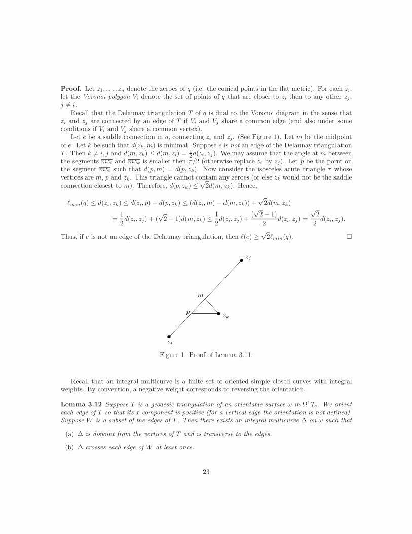
Proof. Let z1, . . . , zn denote the zeroes of q (i.e. the conical points in the flat metric). For each zi,let the Voronoi polygon Vi denote the set of points of q that are closer to zi then to any other zj ,j 6= i.

Recall that the Delaunay triangulation T of q is dual to the Voronoi diagram in the sense thatzi and zj are connected by an edge of T if Vi and Vj share a common edge (and also under someconditions if Vi and Vj share a common vertex).

Let e be a saddle connection in q, connecting zi and zj . (See Figure 1). Let m be the midpointof e. Let k be such that d(zk,m) is minimal. Suppose e is not an edge of the Delaunay triangulationT . Then k 6= i, j and d(m, zk) ≤ d(m, zi) =

12d(zi, zj). We may assume that the angle at m between

the segments mzi and mzk is smaller then π/2 (otherwise replace zi by zj). Let p be the point onthe segment mzi such that d(p,m) = d(p, zk). Now consider the isosceles acute triangle τ whosevertices are m, p and zk. This triangle cannot contain any zeroes (or else zk would not be the saddleconnection closest to m). Therefore, d(p, zk) ≤

√2d(m, zk). Hence,

ℓmin(q) ≤ d(zi, zk) ≤ d(zi, p) + d(p, zk) ≤ (d(zi,m)− d(m, zk)) +√2d(m, zk)

=1

2d(zi, zj) + (

√2− 1)d(m, zk) ≤

1

2d(zi, zj) +

(√2− 1)

2d(zi, zj) =

√2

2d(zi, zj).

Thus, if e is not an edge of the Delaunay triangulation, then ℓ(e) ≥√2ℓmin(q).

zi

zj

zk

m

p

Figure 1. Proof of Lemma 3.11.

Recall that an integral multicurve is a finite set of oriented simple closed curves with integralweights. By convention, a negative weight corresponds to reversing the orientation.

Lemma 3.12 Suppose T is a geodesic triangulation of an orientable surface ω in Ω1Tg. We orienteach edge of T so that its x component is positive (for a vertical edge the orientation is not defined).Suppose W is a subset of the edges of T . Then there exists an integral multicurve ∆ on ω such that

(a) ∆ is disjoint from the vertices of T and is transverse to the edges.

(b) ∆ crosses each edge of W at least once.

23

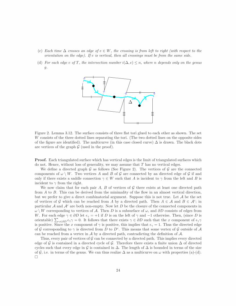
(c) Each time ∆ crosses an edge of e ∈ W , the crossing is from left to right (with respect to theorientation on the edge). If e is vertical, then all crossings must be from the same side.

(d) For each edge e of T , the intersection number i(∆, e) ≤ n, where n depends only on the genusg.

∆

Figure 2. Lemma 3.12. The surface consists of three flat tori glued to each other as shown. The setW consists of the three dotted lines separating the tori. (The two dotted lines on the opposite sidesof the figure are identified). The multicurve (in this case closed curve) ∆ is drawn. The black dotsare vertices of the graph G (used in the proof).

Proof. Each triangulated surface which has vertical edges is the limit of triangulated surfaces whichdo not. Hence, without loss of generality, we may assume that T has no vertical edges.

We define a directed graph G as follows (See Figure 2). The vertices of G are the connectedcomponents of ω \W . Two vertices A and B of G are connected by an directed edge of G if andonly if there exists a saddle connection γ ∈ W such that A is incident to γ from the left and B isincident to γ from the right.

We now claim that for each pair A, B of vertices of G there exists at least one directed pathfrom A to B. This can be derived from the minimality of the flow in an almost vertical direction,but we prefer to give a direct combinatorial argument. Suppose this is not true. Let A be the setof vertices of G which can be reached from A by a directed path. Then A ∈ A and B ∈ Ac; inparticular A and Ac are both non-empty. Now let D be the closure of the connected components inω \W corresponding to vertices of A. Then D is a subsurface of ω, and ∂D consists of edges fromW . For each edge γ ∈ ∂D let ǫγ = +1 if D is on the left of γ and −1 otherwise. Then, (since D isorientable)

∑γ∈∂D ǫγγ = 0. It follows that there exists γ ∈ ∂D such that the x component of ǫγγ

is positive. Since the x component of γ is positive, this implies that ǫγ = 1. Thus the directed edgeof G corresponding to γ is directed from D to Dc. This means that some vertex of G outside of Acan be reached from a vertex in A by a directed path, contradicting the definition of A.

Thus, every pair of vertices of G can be connected by a directed path. This implies every directededge of G is contained in a directed cycle of G. Therefore there exists a finite union ∆ of directedcycles such that every edge in G is contained in ∆. The length of ∆ is bounded in terms of the sizeof G, i.e. in terms of the genus. We can thus realize ∆ as a multicurve on ω with properties (a)-(d).

24

Lemma 3.13 There exist ρ1 > 0 and C > 0 depending only on K such that for any q ∈ π−1(K)there exists q′ ∈ π−1(K) ∩ Fuu(q) and a path γ : [0, ρ1] → Fuu(q) such that γ(0) = q, γ(ρ1) = q′,and for t ∈ [0, ρ1],

ℓmin(γ(t)) ≥ ℓmin(γ(0))√1 + t2, (3.18)

and also

dH(q, q′) ≤ C

∫ ρ1

0

| log(ℓmin(q)√1 + t2)|1/2dt. (3.19)

Proof. Let S = (X, ω) denote the double cover corresponding to q. Consider the Delaunaytriangulation of S. By Lemma 3.11, all saddle connections of length at most

√2ℓmin(S) belong to

the Delaunay triangulation. Let W denote this set of saddle connections. Let ∆ be the multicurveobtained by applying Lemma 3.12 to S and W .

Let τ be the involution corresponding to q. Let ∆′ = ∆ − τ(∆). Then ∆′ also has properties(a)-(d) of Lemma 3.12. In addition, τ(∆′) = −∆′.

Let ρ1 ∈ (0,√2) be a constant which will be chosen later (depending only on the genus). We

now use ∆′ to define a path γ : [0, ρ1] → Q1Tg contained in π−1(K) and staying on the same leafof Fuu. We will actually define the path γ(t) where for each t, γ(t) is the double cover of γ(t). LetS denote the double cover of q, and set γ(0) = S. For each t ∈ [0, ρ1], γ(t) is built from the sametriangles as S, but for each edge e, we add I(e,∆′)tℓmin(q) to the x-component, where I(·, ·) denotesthe algebraic intersection number (cf. [MasSm91, §6]).

Note that we do not assert that the Delaunay triangulation of γ(t) is the same as that of S = γ(0).However, because of the form of ∆′, the involution τ acts on γ(t), and we can let γ(t) be the quotientby τ .

We now claim that (3.18) holds. Indeed, if e ∈ W is a saddle connection in γ(0) with vector(x0, y0), then x0 ≥ 0, and on γ(t), e has length

√y20 + (x0 + I(e,∆′)ℓmin(q)t)2 ≥

√ℓmin(q)2 + ℓmin(q)2t2 = ℓmin(q)

√1 + t2. (3.20)

Suppose t1, t2 ∈ [0, ρ1] and η are such that η is a saddle connection on γ(t) for t1 < t < t2. Let ℓt(η)denote the length of η in the flat metric on γ(t). Then,

ℓt(η) ≥ ℓt1(η)− |I(η,∆)|ℓmin(q)(t− t1). (3.21)

Now suppose z and w be any two zeroes of q. Let λt(z, w) denote the shortest path between zand w on γ(t), and let |λt(z, w)| denote the length of λt(z, w), i.e. the distance between z and win the flat metric on γ(t). Suppose λ0(z, w) is not an edge in W . Then, either λ0(z, w) is a saddleconnection not in W , in which case |λ0(z, w)| ≥

√2ℓmin(q), or λ0(z, w) is a union of at least two

saddle connections, so that |λ0(z, w)| ≥ 2ℓmin(q) ≥√2ℓmin(q). It now follows from (3.21) that for

all t ∈ [0, ρ1],

|λt(z, w)| ≥ (√2− nmt)ℓmin(q),

where n is the maximum intersection number of ∆′ with a saddle connection in the Delaunaytriangulation of S, and m is the maximal number of saddle connections in λt(z, w). Note that bothn and m are bounded by the genus. Now we choose ρ1 so that

√2 − nmρ1 ≥ (1 + ρ1)

2. Then, ifλ0(z, w) is not a saddle connection in W , then for all t ∈ [0, ρ1],

|λt(z, w)| ≥ ℓmin(γ(0))√1 + t2. (3.22)

25

Now (3.18) follows from (3.20) and (3.22).We now estimate the Hodge length of the path γ : [0, ρ1] → Q1Tg. By Lemma 3.4 and Lemma 3.5,

ℓγ(t)(σ) ≥Cg

| log(ℓmin(q)√1 + t2)|

,

where ℓσ(S) is defined to be the infimum over all simple closed curves α of ℓα(σ) (and σ is thehyperbolic metric in the conformal class of S). By construction, the intersection number of ∆′ witha short basis (see §3.3.2) of γ(t) is bounded depending only on the genus. Therefore, by (3.9) and(3.10),

‖γ′(t)‖′ ≤ C| log(ℓmin(q)√1 + t2)|1/2,

where C depends only on the genus. Thus, if q1 = γ(ρ1), then

dH(q, q1) ≤∫ ρ1

0

‖γ′(t)‖′ dt ≤∫ ρ1

0

C| log(ℓmin(q)√

1 + t2)|1/2 dt.

Thus (3.19) holds.

Lemma 3.14 There exists ǫ0 > 0 (depending on K) such that for all ǫ < ǫ0 and for all q ∈ π−1(K)with ℓmin(q) < ǫ, there exists q′ on the same leaf of Fuu as q with ℓmin(q

′) ≥ ǫ, and dH(q, q′) ≤kǫ| log ǫ|1/2, where k depends only on K.

Proof. We define a sequence qn as follows: let q0 = q. If qn has been defined already, we applyLemma 3.13 with q = qn, and define qn+1 to be the point q′ guaranteed by Lemma 3.13. We obtaina sequence qn with

ℓmin(qn+1) ≥ ℓmin(qn)(1 + ρ21)1/2 = ρ2ℓmin(qn),

where we let ρ2 = (1+ρ21)1/2. Define tn inductively by t0 = 0, tn+1 = tn+ρ1ℓmin(qn), n ≥ 0. Then,

tn = ρ1

n−1∑

k=0

ℓmin(qk) ≤ ρ1

n−1∑

k=0

ℓmin(qn)

ρn−k2

= ρ1ℓmin(qn)ρ−12 − ρ−n−1

2

1− ρ−12

≤ ρ1ℓmin(qn)

ρ2 − 1.

Then,

tn+1 = tn + ρ1ℓmin(qn) ≤ρ1ρ2ρ2 − 1

ℓmin(qn).

Thus, for t ∈ [tn, tn+1],

ℓmin(qn) ≥ρ2 − 1

ρ1ρ2t ≡ ρ3t.

We have

dH(qn, qn+1) ≤∫ tn+1

tn

C| log(ℓmin(qn)√1 + t2)|1/2 dt ≤

∫ tn+1

tn

C| log(ρ3t√1 + t2)|1/2 dt.

Thus,

dH(q0, qn) ≤∫ tn

0

C| log(ρ3t√1 + t2)|1/2 dt.

26

We choose n so that ℓmin(qn) is comparable to ǫ. Let q′ = γ(tn). Then, ℓmin(q′) ≥ tn ≈ ǫ. Now the

modified Hodge length of the path q0, q1, . . . , qn is O(ǫ| log ǫ|1/2).

Proof of Theorem 3.10. Since K is compact, the intersection of the multiple zero locus withπ−1(K) is (contained in) finite union of hyperplanes H1, . . . , Hn. Each hyperplane Hj has complexcodimension 1. We can choose ǫ0 > 0 such that any two Hj which do not intersect in π−1(K) are atleast ǫ0 apart. Let δ0 > 0 be a lower bound on the angle between any two Hj which do intersect inπ−1(K). Clearly ǫ0 and δ0 depend only on K.

Let Z be the locus where our quadratic differential has either a zero of order at least 3 or twozeroes each of order at least 2. Then there exists a constant k0 (depending only on δ0 and thusonly on K) such that for any q ∈ π−1(K) and any ǫ > 0, if the ball BE(q, ǫ) intersects at least twohyperplanes Hj then dE(q, Z) < k0ǫ.

Take two points q1, q2 ∈ π−1(K) on the same leaf of Fuu, with d(q1, q2) = ǫ. Choose k3 > k0(thus k3 depends only on K). We also assume that k3ǫ < ǫ0. By Lemma 3.14 (with k3ǫ in placeof ǫ), there exist q′1, q

′2 so that for i = 1, 2, we have dH(qi, q

′i) ≤ k1ǫ| log ǫ|1/2, dE(qi, q′i) ≤ k2ǫ, and

ℓmin(qi) = k3ǫ, where k1, k2 depend only on K. Since k3 > k0 and k3ǫ < ǫ0, there exist ǫ1, ǫ′1 such

that k3ǫ/2 > ǫ1 > ǫ′1 > ǫ/(2k3), and for all q ∈ π−1(K), either dE(q, Z) < ǫ1 or BE(q, ǫ′1) contains

at most one hyperplane from the multiple zero locus.Note that the intersection of Z with π−1(K) has complex codimension at least 2. Hence, the

intersection of the ǫ1-neighborhood of Z with Fuu(q1)∩π−1(K) is contained in the ǫ1-neighborhoodof a finite union of hyperplanes, each of real codimension at least 2. Then there exists a constantk4 depending only on K, and a path γ connecting q′1 to q′2 of length at most k4ǫ, which avoids theǫ1-neighborhood of Z.

Now let p0 = q′1, and mark points pi along γ which are ǫ′1/2 apart in the Euclidean metric. Wehave pn = q′2. Let Bi be the ball of Euclidean diameter ǫ′1/2 which contains pi and pi+1 on itsboundary. By construction Bi contains at most one hyperplane (which we will denote L) from themultiple zero locus. Note that by Lemma 3.4, Lemma 3.5 and (3.12), for any p ∈ Bi and any tangentvector v at p, the modified Hodge norm of v can be estimated as

‖v‖′H ≤ C| log dE(p, L)|1/2‖v‖E, (3.23)

where ‖v‖E is the Euclidean norm of v, and d(p, L) denotes the Euclidean distance between thepoint p and the hyperplane L.

Let p′i be the farthest point in Bi from the hyperplane. Then, after connecting pi and p′i by a

straight line path and using (3.23), we see that dH(pi, p′i) = O(ǫ| log ǫ|1/2), and also dH(p′i, pi+1) =

O(ǫ| log ǫ|1/2). Thus, since the number of Bi along the path is bounded by a constant dependingonly on K, we finally obtain

dH(q′1, q′2) = O(dE(q

′1, q

′2)| log ǫ|1/2).

3.6 The Non-expansion and Decay of the Hodge Distance.

Theorem 3.15 Suppose q ∈ Q1Tg and q′ ∈ Q1Tg are in the same leaf of Fss. Then

27

(a) There exists a constant cH > 0 such that for all t ≥ 0,

dH(gtq, gtq′) ≤ cHdH(q, q′).

(b) Suppose ǫ > 2ǫ1, where ǫ1 is as in the definition of short basis (see §3.3.2). Let K = q ∈Q1Tg : ℓmin(q) > ǫ. Suppose dH(q, q′) < 1, and t > 0 is such that

|s ∈ [0, t] : gsq ∈ ΓK| ≥ (1/2)t. (3.24)

Then for all 0 < s < t,dH(gsq, gsq

′) ≤ Ce−csdH(q, q′),

where c and C depend only on g and ǫ.

Proof. The statement (a) follows immediately from Theorem 3.6. For the second statement, letγ : [0, ρ] → Q1Tg be a modified Hodge length minimizing path connecting q to q′ (and staying inthe same leaf of Fss). We assume that γ is parametrized so that dH(γ(u), q) = u. By assumption,ρ < 1.

Let N = 4cH/(c1ǫρ), where c1 is as in Theorem 3.10. For 0 ≤ j ≤ N , let uj = jc1ǫ/(4cH). Wenow claim that for all j there exists tj such that for s > tj such that gsq ∈ ΓK, we have for all0 ≤ u < uj ,

dE(gsγ(u), gsq) < ǫ

j∑

k=0

2−k, (3.25)

anddH(gsγ(u), gsq) < Ce−csu, (3.26)

where C and c depend only on g and ǫ. The equations (3.25) and (3.26) will be proved by inductionon j. If j = 0 then there is nothing to prove. Now assume j ≥ 1, and (3.25) and (3.26) are true forall u ≤ uj−1. Suppose u < uj. By (a), we have for all t > 0,

dH(gtγ(u), gtγ(uj−1)) < cH(u− uj−1) < c1ǫ/4.

Therefore by Theorem 3.10, dE(gtγ(u), gtγ(uj−1)) < ǫ/2. Therefore, by the inductive assumption(3.25), for the s > tj−1 such that gsq ∈ ΓK, for all uj−1 < u < uj, we have ℓmin(gsγ(u)) > ǫ/2.Thus, by (3.14), for all uj−1 < u < uj, the modified Hodge norm of γ′(u) is within a constant of theHodge norm of γ′(u). Then by Theorem 3.3, for all uj−1 < u < uj ,

dH(gtγ(u), gtγ(uj−1)) < Ce−ctdH(γ(u), γ(uj−1)). (3.27)

Therefore, by Theorem 3.10, there exists tj > 0 (depending only on g and ǫ) such that for s > tjwith gsq ∈ ΓK, and uj−1 ≤ u < uj, (3.25) holds. Also (3.26) follows from (3.27). The inductionterminates after finitely many steps (depending only on g and ǫ). Thus (b) holds.

28

4 The multiple zero locus.

In this section we prove Theorem 2.6 and Theorem 2.7.Let K be a compact subset of Tg. We assume that K is contained in one fundamental domain

for the action of Γ on Tg (and thus we can identify K with a subset of Mg). All of our impliedconstants will depend on K.

Notation. Suppose W ⊂ Q1Tg and s > 0. Let W (s) denote the set of q ∈ Q1Tg such that thereexists q′ ∈ W on the same leaf of Fuu as q such that dH(q, q′) < s. Recall that for a subset A ⊂ Tg,Nbhdr(A) denotes the set of points within Teichmuller distance r of A. We will also use A(r) todenote Nbhdr(A). Let ν and η+ be as in §2.2, so that so that for a set F contained in a leaf of Fuu,ν(η+(F )) = µαuu(F ).

Lemma 4.1 Suppose U ⊂ π−1(K), δ > 0 and t > 0. Let W = gtU ∩Γπ−1(K). There is a C(δ) > 0so that

m(Nbhd2(π(W ))) ≤ C(δ)ν(η+(W (δ))), (4.1)

(By our convention, the constant C(δ) depends on K as well). Also

ν(η+(W (1))) ≤ C(δ)ν(η+(W (δ))). (4.2)

Proof. Let δ0 = δ0(K, δ) be a constant to be chosen later. We decompose U into pieces Uα suchthat each piece is within (modified) Hodge distance δ0/2 of a single leaf of Fuu. Let

Wα = gtUα ∩ Γπ−1(K).

Thenm(Nbhd2(π(W ))) ≤

∑

α

m(Nbhd2(π(Wα)))

In view of Theorem 3.10 the number of pieces is bounded depending only on K and δ (since δ0 =δ0(K, δ)). Thus, it is enough to show that (4.1) holds with W replaced by Wα.

We now claim that without loss of generality, we may assume that Uα has the following “productproperty”: given q1, q2 ∈ Uα, there exists q′2 ∈ Uα on the same leaf of Fuu as q1 and on the sameleaf of Fs as q2. If not, let

U ′α = Uα ∪ Fuu(q1) ∩ Fs(q2) : q1, q2 ∈ Uα.

Then η+(Uα) = η+(U ′α), and therefore η+(gtUα) = η+(gtU

′α). Also if δ′ = δ′(δ,K) is sufficiently

small then W ′α = gtU

′α ∩Γπ−1(K) satisfies W ′

α(δ′) ⊂Wα(δ). Therefore we can proceed with the rest

of the proof with δ′ instead of δ and U ′α instead of Uα. Therefore, without loss of generality, we may

assume that Uα has the product property. Therefore, gtUα also has the product property.Pick a maximal ∆ ⊂ π(Wα) such that for any two distinct X,Y ∈ ∆, dT (X,Y ) = 1. Then,

Nbhd2(π(Wα)) ⊂⋃

X∈∆

Bτ (X, 3),

and hence,

m(Nbhd2(π(Wα))) ≤ m

( ⋃

X∈∆

Bτ (X, 3)

)≤∑

X∈∆

m(B(X, 3)) ≤ C(K)|∆|, (4.3)

29

where |∆| denotes the cardinality of ∆, and we have used the fact that ∆ ⊂ ΓK.For each X ∈ ∆, pick one q ∈ Wα ∩ π−1(X). Let ∆′ ⊂ Wα denote the resulting set of q’s. Let

BuuE (q, r) denote the set of q′ ∈ Q1Tg on the same leaf of Fuu as q with dE(q, q

′) < r. We claimthat for δ0 sufficiently small, we can pick δ2 depending only on K such that for all distinct pairsq1, q2 ∈ ∆′,

η+(BuuE (q1, δ2)) ∩ η+(Buu

E (q2, δ2)) = ∅. (4.4)

To prove (4.4), suppose q1, q2 ∈ ∆′, and q1 6= q2. Let q′2 be such that q1 and q

′2 are on the same leaf of

Fuu and q2 and q′2 are on the same leaf of Fs. By Theorem 3.15, we have dH(q2, q′2) < cHδ0. There-

fore, by Theorem 3.10 and Lemma 3.9, we can choose δ0 small enough so that dT (π(q2), π(q′2)) ≤ 1/5.

Hence, π(q′2) ⊂ ΓK′ where K′ ⊂ Tg is compact, and by the triangle inequality,

dT (π(q1), π(q′2)) ≥ dT (π(q1), π(q2))− dT (π(q2), π(q

′2)) ≥ 4/5. (4.5)

By Lemma 3.9, there exists δ1 > 0 (depending only on K′) such that for all q, q′ ∈ K′ on the sameleaf of Fuu with dE(q, q

′) < δ1, we have dT (π(q), π(q′)) < 1/5. Then, by (4.5) and the triangle

inequality, BuuE (q1, δ1) and B

uuE (q′2, δ1) are disjoint. It follows that as subsets of PMF ,

η+(BuuE (q1, δ1)) ∩ η+(Buu

E (q′2, δ1)) = ∅ (4.6)

Let Fs(q) denote the leaf of Fs through q. Since η+ is continuous and K′ is compact, there existconstants 0 < δ2 < δ1 and δ3 > 0 (depending only on K′) such that for all q, q′ ∈ K′ with q ∈ Fs(q′)and dH(q, q′) < δ3, we have, as subsets of PMF ,

η+(BuuE (q, δ2)) ⊂ η+(Buu

E (q′, δ1)).

We now choose δ0 < δ3/cH . Then, since q2 and q′2 are on the same leaf of Fs and dH(q2, q′2) <

cHδ0 < δ3, we haveη+(Buu

E (q2, δ2)) ⊂ η+(BuuE (q′2, δ1)).

Now using (4.6), we get that as subsets of PMF ,

η+(BuuE (q1, δ2)) ∩ η+(Buu

E (q2, δ2)) ⊂ η+(BuuE (q1, δ1)) ∩ η+(Buu

E (q′2, δ1)) = ∅.

This completes the proof of (4.4).By Theorem 3.10, there exists 0 < δ3 < δ2 such that for all q ∈ ∆′ and all q′ ∈ Fuu(q) with

dE(q, q′) < δ3 we have dH(q, q′) < δ. For q ∈ ∆′, let

H(q) = η+(BE(q, δ3)) ⊂ η+(W (δ)),

Consider the collection of “balls” H(q) : q ∈ ∆′. By (4.4) the sets H(q) are pairwise disjointviewed as subsets of PMF (or alternatively the subsets Cone(H(q)) ⊂ MF intersect only at theorigin). Also, by the definition of the Thurston measure ν and the compactness of K, there exists aconstant c = c(K, δ) such that

ν(H(q)) ≥ c, for all q ∈ ∆′.

Hence,

ν(η+(W (δ))) ≥ ν

⋃

q∈∆′

H(q)

=

∑

q∈∆′

ν(H(q)) ≥ c|∆′| = c|∆|. (4.7)

30

Now (4.1) (with W replaced by Wα) follows from (4.3) and (4.7). Finally,

ν(η+(W (1))) ≤ C(δ,K)ν(η+(W (δ))),

since dH is equivalent to dE .

The sets Ki and Ui. Let K1 ⊂ Q1Mg be a compact set. (In our application, K1 will be chosendisjoint from the multiple zero locus). Let K3 ⊂ K2 ⊂ K1 and 1 ≥ δ > 0 be such that if q ∈ Ki anddH(q, q′) < cHδ then q′ ∈ Ki−1, where cH is as in Theorem 3.15 (a). We assume µ(K3) > (1/2),where µ is the normalized Lebesgue measure on Q1Mg. For T0 > 0 let Ui = Ui(T0) be the set ofq ∈ Q1Mg such that there exists T > T0 so that

|t ∈ [0, T ] : gtq ∈ Kci | ≥ (1/2)T.

Then, for all T > T0 and all q 6∈ Ui,

|t ∈ [0, T ] : gtq ∈ Kci | < (1/2)T. (4.8)

From the definition, we have U1 ⊂ U2 ⊂ U3. By the ergodicity of the geodesic flow, for every θ > 0there exists T0 > 0 such that µ(U3) < θ.

Let K1 = K. We can choose compact subsets K0, K2, K3 of Tg such that for 0 ≤ i ≤ 2, anyq ∈ π−1(Ki) and any q′ on the same leaf of Fuu as q with dH(q, q′) < cH , we have q′ ∈ π−1(Ki+1). By(the lower bound in) Theorem 3.10 and Lemma 3.9, each Ki is compact. Let U ′

i = p−1(Ui)∩π−1(Ki),where p is the natural map from Q1Tg to Q1Mg. Note that U ′

1 ⊂ U ′2 ⊂ U ′

3 ⊂ Q1Tg.

Lemma 4.2 Let U ′i , 1 ≤ i ≤ 3 be as in the above paragraph. Then, for all t > 0,

m(Nbhd2(π(gtU′1) ∩ ΓK)) ≤ C(δ)ehtν(η+(U ′

2)),

and if W (1) is defined as in Lemma 4.1 with W = gtU′1 ∩ π−1(ΓK), then

ν(η+(W (1))) ≤ C′(δ)ehtν(η+(U ′2)).

In particular (c.f. Theorem 2.2), for any ǫ > 0 is is possible to choose T0 such that if U1 is definedby (4.8) and U ′

1 = U1 ∩ π−1(K1) then for all t > T0,

m(Nbhd2(π(gtU′1)) ∩ ΓK) ≤ ǫeht, (4.9)

and for W = gtU′1 ∩ π−1(ΓK) we have

ν(η+(W (1))) ≤ ǫeht. (4.10)

Proof. We will apply Lemma 4.1 to the set W = gtU′1 ∩ π−1(ΓK). We claim that W (δ) ⊂ gtU

′2.

Indeed, suppose gtq′ ∈ W (δ). Then there exists gtq ∈W with

dH(gtq, gtq′) < δ.

Then, by Theorem 3.15 (a), for all 0 ≤ s ≤ t,

dH(gsq, gsq′) < cHδ (4.11)

31

Since W = gtU′1, gtq ∈ W implies q ∈ U ′

1. Then, assuming t > T0, for at least half the values ofs ∈ [0, t],

gsq 6∈ K1. (4.12)

Then, (4.11) and the definition of K2 imply that for the s ∈ [0, t] for which (4.12) holds, gsq′ 6∈ K2.

This implies q′ ∈ U2. Since dH(q, q′) < cHδ < cH and q ∈ π−1(K) = π−1(K1), we have q′ ∈ π−1(K2).

Thus, q′ ∈ U2 ∩ π−1(K2) = U ′2, and so gtq

′ ∈ gtU2. This implies the claim, and thus the first twostatements of the Lemma.

The same argument as the proof of the claim shows that if q ∈ U ′2 and q′ ∈ Fss(q)∩π−1(K) with

dH(q, q′) < δ then q′ ∈ U ′3. This (together with Theorem 3.10) implies that there exists C1(δ) such

thatν(η+(U ′

2)) ≤ C1(δ)µ(U′3).

Hence if we choose T0 > 0 so that µ(U3) < C(δ)C1(δ)ǫ, then (4.9) follows. Similarly, if we chooseT0 > 0 so that in addition µ(U3) < C′(δ)C1(δ)ǫ, then (4.10) follows.

Proof of Theorem 2.7. Let K ′ = K1, and let T0, U1 and U ′1 be as in Lemma 4.2. Then, for

R > T0, and X ∈ K,

BR(X,K,K ′) ⊂⋃

0≤t≤R

π(gtU′1) ∩ ΓK ⊂

⌊R⌋⋃

n=0

⋃

t∈[n,n+1]

π(gtU′1) ∩ ΓK,

where ⌊x⌋ denotes the integer part of x. Then,

m(Nbhd1(BR(X,K,K ′))) ≤⌊R⌋∑

n=0

m(Nbhd2(π(gnU′1) ∩ ΓK)) ≤ Cǫ

⌊R⌋∑

n=0

ehn,

where we have used (4.9). Since ǫ is arbitrary, Theorem 2.7 follows.

Lemma 4.3 Suppose V ⊂ π−1(K) and δ′ > 0. Then, for t sufficiently large (depending on K, Vand δ′),

m(Nbhd1(π(gtV ) ∩ ΓK0)) ≤ Cν(η+(V (δ′)))eht,

where C depends only on K.

Proof. Let Y = gtV ∩ ΓK0. Choose T0 so that (4.10) holds for t > T0 and ν(η+(V (δ′))) instead ofǫ. Let U1, U

′1 and W = gtU

′1 ∩ π−1(K) be as in Lemma 4.2, so in particular, for t > T0,

ν(η+(W (1))) ≤ ν(η+(V (δ′)))eht. (4.13)

We claim that there exist T1 > T0, depending only on K such that for t > T1,

Y (1) =W (1) ∪ gt(V (δ′)). (4.14)

Indeed, if gtq ∈ Y (1) then by definition there exists q′ ∈ V ⊂ K with dH(gtq, gtq′) < 1, and q′

is on the same leaf of Fuu as q. We consider two cases: either q′ ∈ U1 or q′ 6∈ U1. If q′ ∈ U1 then

32

q ∈ U ′1 = U1 ∩ K, hence gtq

′ ∈ gtU′1 ∩ ΓK = W . Hence in this case, gtq ∈ W (1). If q′ 6∈ U1, then by

(4.8) and Theorem 3.15 (b),

dH(q, q′) = dH(g−tgtq, g−tgtq′) ≤ Ce−ctdH(gtq, gtq

′) ≤ Ce−ct.

We choose T1 > T0 so that Ce−cT1 < δ′. Thus, in this case, for t > T1, q ∈ V (δ′) and hence (4.14)follows.

Now, for t > T1,

ν(η+(Y (1))) ≤ ν(η+(W (1))) + ν(η+(gt(V (δ′)))) ≤ 2ν(η+(V (δ′)))eht

where we have used (4.13). We now apply Lemma 4.1 with δ = 1. The lemma follows from (4.1).

Proof of Theorem 2.6. This follows immediately from Lemma 4.3, and the fact that we canchoose an relatively open V ⊂ K and δ′ > 0 such that V contains the intersection of K with themultiple zero locus, and ν(η+(V (δ′))) is arbitrarily small, (see Theorem 2.2).

5 Volume Asymptotics.

In this section we prove Theorem 1.3. Let FR(X,Y ) = |Γ · Y ∩BR(X)| be as in §2.6. We need thefollowing:

Theorem 5.1 Given X ∈ Tg there exists C = C(X) such that for all Y ∈ Tg,

FR(X,Y ) ≤ C(X)ehR.

Notation.

• Let Cg(N) be the set of isotopy classes of integral multicurves on a surface of genus g.

• Given X,Y ∈ Tg define

MR(X,Y ) = γ · Y, γ ∈ Γ | γ · Y ∈ BR(X),

so that FR(X,Y ) = #(MR(X,Y )).

Proof of Theorem 1.3 assuming Theorem 5.1. By definition of FR,

m(BR(X)) =

∫

Mg

FR(X,Y ) dm(Y )

We multiply both sides by e−hR and take the limit at R → ∞. By Theorem 5.1 we can apply thebounded convergence theorem to take the limit inside the integral. Now the theorem follows fromTheorem 1.2.

A similar argument yields the following:

33

Theorem 5.2 Suppose X ∈ Tg, and U ⊂ S(X). Then, as R → ∞,

m(BR(X) ∩ SectU(X)) ∼ 1

hm(Mg)ehRΛ(Y )

∫

U

λ−(q) dsX(q).

In the rest of this section we prove Theorem 5.1. Along the way, we prove Theorem 2.4.

Estimating extremal lengths. Consider the Dehn-Thurston parameterization [HP92] of the setof multicurves

DT : Cg(N) → (Z+ × Z)3g−3

defined byDT (β) = (i(β, αi), tw(β, αi))

3g−3i=1 ,

where i(·, ·) denotes the geometric intersection number and tw(β, αi) is the twisting parameter of βaround αi. See [HP92] for more details. By a theorem of Bers, we can choose a constant Cg dependingonly on g such that for any surface Y ∈ Tg there exists a pants decomposition P = α1, . . . , α3g−3on Y such that for 1 ≤ i ≤ 3g − 3

Extαi(Y ) ≤ C2

g .

We call such a pants decomposition a bounded pants decomposition for Y. The following result isproved in [Mi96] (see Theorem 5.1, and equation (4.3)):

Theorem 5.3 (Minsky) Suppose Y ∈ Tg, and let P = P(Y ) = α1, . . . , α3g−3 be any boundedpants decomposition on Y . Then given a simple closed curve β, Extβ(Y ) is bounded from above andbelow by

max1≤j≤3g−3

[i(β, αj)

2

Extαj(Y )

+ tw2(β, αj)Extαj(Y )

], (5.1)

up to a multiplicative constant depending only on g.

Theorem 5.3 gives a bound on the the Dehn-Thurston coordinates of a simple closed curve interms of its extremal length.

Remark. The definition of the twist used in equation (4.3) in [Mi96] is different from the definitionwe are using here. We follow the definition used in [HP92]. Given a connected simple closed curveα on Σg, let hα ∈ Γ denote the right Dehn twist around α. Then in terms of our notation,

tw(hrα(β), α) = tw(β, α) + r · i(β, α). (5.2)

Corollary 5.1 Let α = α1, . . . , α3g−3 be bounded pants decomposition of X ∈ Tg. Then there isa constant c1 > 0 such that for any simple closed curve β on Σg,

tw(β, αi) ≤ c1 ·√Extβ(X)√Extαi

(X),

and

i(β, αi) ≤√Extβ(X) ·

√Extαi

(X) ≤ c1

√Extβ(X).

34

Estimating the number of multicurves. Define

E(Y, L) = #|α ∈ Cg(N) |√Extα(Y ) ≤ L|

Fix ǫ0 > 0 small enough such that if α and β on Y ∈ Tg satisfy Extα(Y ) ≤ ǫ20 and Extβ(Y ) ≤ C2g

then i(α, β) = 0. Note that any bounded pants decomposition P on Y includes all simple closedcurves of extremal length ≤ ǫ20 on Y.

Let

G(Y ) = 1 +∏

Extγ(Y )≤ǫ20

1√Extγ(Y )

,

and the product ranges over all simple closed curves γ on the surface Y with Extγ(Y ) ≤ ǫ20.Using Theorem 5.3, we obtain the following:

Theorem 5.4 There exists a constant C > 0 such that for every Y ∈ Tg and L > 0 we have

E(Y, L) ≤ C ·G(Y ) · L6g−6.

Moreover, for any Y , if 1/L is bounded by an absolute constant times the square root of the extremallength of the shortest curve on Y , then

E(Y, L) ≤ CL6g−6.

Sketch of the proof. In order to use the bound given by equation (5.1), first we fix a boundedpants decomposition

P = α1, . . . , α3g−3on Y . Note that, this pants decomposition should include all small closed curves on Y. Let mi =i(β, αi), ti = tw(β, αi), and si =

√Extαi

(Y ). So by equation (5.1), Extβ(Y ) ≤ L2 implies thatmi

si+ |ti|si = O(L). We use the following elementary lemma:

Lemma 5.5 For s > 0, define As(L) by

As(L) = (a, b) | a, b ∈ Z+, a · s+b

s≤ L ⊂ Z+ × Z+.

Then for any L > 0, |As(L)| ≤ 4maxs, 1/s · L2. For L > maxs, 1s, we have As(L) ≤ 4L2.

Now applying the preceding lemma to the si, and using the Dehn-Thurston parameterization ofmulticurves, we get

E(Y, L) ≤3g−3∏

i=1

|Asi (L)| ≤ C G(Y )L6g−6.

Proof of Theorem 2.4. This follows from the second part of Theorem 5.4. Recall (see §2.1) thatthe extremal length can be extended continuously to a map

Ext : MF × Tg → R+

35

such that Exttλ(X) = t2Extλ(X). Also the space MF has a piecewise linear integral structure, andelements of Sg are in one to one correspondence with the integral points. Hence,

Λ(X) = Volη ∈ MF |√Extη(X) ≤ 1 =

Volη ∈ MF |√Extη(X) ≤ L

L6g−6= lim

L→∞

E(x, L)

L6g−6, (5.3)

where to justify the last equality use the fact that for any as L→ ∞ the number of lattice points inthe dilation LA is asymptotic to the volume of LA, where A = η ∈ MF |

√Extη(X) ≤ 1.

On the other hand, by the second assertion in Theorem 5.4 when L is big enough E(Y, L) ≤CL6g−6. Therefore, Λ(Y ) ≤ C, where the bound does not depend on Y.

Remark. Let p : Tg → Mg be the natural projection. Fix a compact subset K ⊂ Mg. Forsimplicity, we will also denote p−1(K) ⊂ Tg by K. If P = αi is a bounded pants decomposition onX ∈ K then for any 1 ≤ i ≤ 3g − 3,

1

CK≤√Extαi

(X) ≤ CK,

where CK is a constant which only depends on K. Therefore, by Corollary 5.1, for the elements inthe thick part of the Teichmuller space, the Dehn-Thurston coordinates of a simple closed curveare bounded by its extremal length. More precisely, if α = α1, . . . , α3g−3 be bounded pantsdecomposition of X ∈ K. then there is a constant c1 > 0, depending only on K, such that for anysimple closed curve β on Σg,

tw(β, αi) ≤ c1 ·√Extβ(X), i(β, αi) ≤ c1 ·

√Extβ(X).

Proposition 5.6 There exists a constant C3 depending only on K such that for every X ∈ K,Y ∈ Tg and R > 0 we have

FR(X,Y ) ≤ C3 E(Y, eR).

Our goal is to assign to any point Z = γ · Y ∈ MR(X,Y ) a unique integral multicurve βZ ∈E(Y, eR). This would imply that

FR(X,Y ) ≤ Ce(6g−6)R.

(Note that we are assuming that X is in the compact part of Tg and d(X,Y ) < R; this implies thatthe shortest curve on Y has extremal length at least constant times e−2R, hence we may use thesecond statement of Theorem 5.4.)

The most natural candidate for βZ is γ−1α where α is a fixed pants decomposition of X . Howeverthis correspondence is not one to one. Therefore, we need to modify the construction.

Given Z = γ · Y ∈MR(X,Y ), and α ∈ Sg we have

√Extα(Z)√Extα(X)

≤ eR.

So by setting L = eR, and β = γ−1(α) we have

√Extβ(Y ) ≤ L ·

√Extα(X). (5.4)

36

Given Z = γ · Y ∈MR(X,Y ), let α(Z)i = γ−1αi ∈ Sg. Then from (5.4) we get

√Extα(Z)i(Y ) ≤ CK · L.

Moreover, for Z1 = γ1Y, Z2 = γ2Y ∈ Γ · Y , we have α(Z1) = α(Z2) if and only if there arer1, . . . r3g−3 ∈ Z such that

γ1 = hr1α1· · ·hr3g−3

α3g−3· γ2.

Moreover, we have:

Lemma 5.7 Let α = α1, . . . , α3g−3 be a bounded pants decomposition on X and suppose Y0 ∈BR(X). If hr1α1

· · ·hr3g−3

α3g−3(Y0) ∈ BR(X) then for 1 ≤ i ≤ 3g − 3

|ri| ·√Extαi

(Y0) ≤ C2eR√

Extαi(X)

.

Here C2 is a constant independent of X and Y0.

Sketch of the proof of Lemma 5.7. Let si =√Extαi

(Y0), and L = eR. The key point in theproof is Lemma 6.3 in [Mi96]. From this lemma, for any i, there exists a multicurve βi of extremallength b2i = Extβi

(Y0) such thati(βi, αi) ≥ csi · bi.

Since d(X,Y0) ≤ R,√Extβi

(X) ≤ bi · L. Also the assumption

d(h−r1α1

· · ·h−r3g−3

α3g−3(X), Y0) ≤ R

implies that √Ext

hr1α1

···hr3g−3α3g−3

(βi)(X)) =

√Extβi

(h−r1α1

· · ·h−r3g−3

α3g−3(X)) ≤ bi · L. (5.5)

Then

1. Since√Extβi

(X) ≤ bi · L, Corollary 5.1 implies that the twist and intersection coordinates ofthe curve βi are bounded by a multiple of bi · L; in particular

| tw(βi, αi)| = O

(bi · L√Extαi

(X)

).

2. Similarly, by equation (5.5), applying Corollary 5.1 for hr1α1· · ·hr3g−3

α3g−3(βi) on X with respect to

αi implies that

| tw(hr1α1· · ·hr3g−3

α3g−3(βi), αi)| = O

(bi · L√Extαi

(X)

).

3. On the other hand, by the definition (see equation (5.2)) we have

| tw(hr1α1· · ·hr3g−3

α3g−3(βi), αi)| = |ri · i(αi, βi) + tw(βi, αi)| ≥

≥ |ri| · i(αj , βi)− | tw(βi, αi)|.

37

So we have

|ri| · si · bi ≤1

c|ri| · i(βi, αi) ≤ C2L · bi =⇒ |ri| · si ≤

C2L√Extαi

(X).

Remark. As a result, if the assumption of Lemma 5.7 holds and X ∈ K then

|ri| ·√Extαi

(Y0) ≤ CeR,

where C is a constant which only depends on K.We remark that for any two disjoint simple closed curves η1 and η2, and m1,m2 > 0, we have,

by the definition of extremal length,√Extm1·η1

(X) +√Extm2·η2

(X) ≥√Extm1·η1+m2·η2

(X).

Corollary 5.2 If the assumption of Lemma 5.7 holds and X ∈ K then for α =3g−3∑i=1

|ri| ·αi we have

√Extα(Y0) ≤ C3e

R.

Therefore, α also defines a multicurve of extremal length bounded by e2R. This completes theproof of Proposition 5.6, and thus in view of Theorem 5.4 the proof of Theorem 5.1.

A Appendix: Proof of Theorem 2.2.

In this section,Q∗Tg denotes the space of non-zero quadratic differentials on marked compact surfacesof genus g, without restriction on area.

A local coordinate system near the multiple zero locus. Near the multiple zero locus,the coordinate system given by the period map (see Lemma 3.8) is singular. Instead we use analternative coordinate system from [HuMas79].

Suppose q0 ∈ Q∗Tg has multiple zeroes, say w1, . . . , wm. Let mi be the multiplicity of q0 at wi.Then, by [HuMas79, Proposition 3.1], for 1 ≤ i ≤ m there exists a choice of local coordinate zi,mapping wi to 0, such that any q ∈ Q∗Tg near q0, on a neighborhood of wi, has the form:

q =

zmi

i +

mi−2∑

j=0

aijzji

(dzi)

2.

The coordinates zi are uniquely determined by q. Fix some δ > 0, and let w′i be the point

corresponding to zi = δ. For q ∈ Q∗Tg near q0 let X denote the canonical double cover which makes

the foliations corresponding to q orientable, and let σ be the involution of X so that X/σ is thesurface X (with the flat structure given by q). Let Σδ = σ−1(w′

1, . . . , w′m), and let H denote the

relative homology group H1(X,Σδ,Z). Let Hodd denote the odd part of H under the action of theinvolution σ. Let γ1, . . . , γm be a integral basis for Hodd. Let

λi =

∫

γi

√q.

38

Suppose mi is even. Let wij , 1 ≤ j ≤ mi denote the zeroes of q which tend to wi as q → q0. Letηi be a fixed small circle in the coordinates zi, centered at zi = 0 (i.e. wi). Then if q is sufficientlyclose to q0, ηi separates all the wij from the rest of the surface. Let bi =

∫ηi

√q. Then, a residue

calculation shows that

bi = ami2

−1 + some polynomial in aij , mi − 2 ≥ j ≥ mi

2. (A.1)

Proposition A.1 (Hubbard-Masur) If q0 is not a square of an Abelian differential, then thereexists a neighborhood U ⊂ Q∗Tg of q0 such that the aij and the λi are smooth local coordinates onU . If q0 is the square of an Abelian differential, then there exists a neighborhood U of q0 such thatunder the constraint

∑i bi = 0, the aij and the λi are local coordinates on U .

In both cases, near q0, the natural projection map π : Q∗Tg → Tg is a submersion in thesecoordinates.

Proof. See [HuMas79, Proposition 4.7].

The constraint∑

i bi = 0 appears because in the case when q0 is the square of an Abeliandifferential, the part of the surface which is outside all the circles ηi has an orientable foliation. Inthat case, in view of (A.1), we may drop ami

2−1 for some i from the coordinate system.

We introduce a covering of Q∗Tg by open sets Uα, such that each Uα is the neighborhood Uof Proposition A.1, for some q0 ∈ Q∗Tg. We may assume that the Uα are invariant under theoperation of multiplying the quadratic differential by a real number. We also assume that coveringis uniformly locally finite on compact sets, i.e. that for any compact set K ∈ Tg, there exist a numberN depending only on K such that each point in π−1(K) belongs to at most N sets Uα.

Let ψα be a partition of unity subordinate to Uα. For q, q′ ∈ Uα, let aij, λi be the coordinates

of q, and a′ij , λ′i be the coordinates of q′. Let Dα(q, q′) =

∑ij |aij − a′ij |+

∑i |λi − λ′i|. For q and

q′ sufficiently close so that they belong to the same Uα, let D(q, q′) =∑

α ψαDα(q, q′).

Recall dT (X,Y ) denotes the Teichmuller distance between X and Y , and S(X) denotes thesphere of unit area quadratic differentials which are holomorphic at X .

Lemma A.2 Suppose X, Y in Tg are sufficiently close and belong to a compact set K. Then, thereexist c > 1 depending only on K such that

c−1 infq∈S(X)

D(q, π−1(Y )) ≤ dT (X,Y ) ≤ c supq∈S(X)

D(q, π−1(Y )). (A.2)

Proof. Let K be the pullback of K from Tg to Q1Tg. Then K is also compact. Near any q ∈ K, byProposition A.1, the map π : Q∗Tg → Tg is a submersion, and therefore can be approximated by alinear map, for which (A.2) is immediate. The rest follows by compactness.

Let βα be the measure on Uα ⊂ Q∗Tg given by∏

i,j daij∏

i dλi. Let β =∑

α ψαβα.

For V ⊂ π−1(X), let V ∗ ⊂ Q∗Tg denote the set of all quadratic differentials which have the samehorizontal foliation as some q ∈ V .

Lemma A.3 For every δ > 0, any X ∈ Tg and any q0 ∈ Q∗Tg there exists an open subset V ofπ−1(X) containing q0, such that for all sufficiently small ǫ > 0,

β(V ∗ ∩ π−1(B(X, ǫ))) < δǫ6g−6.

39

Proof. Fix δ′ > 0. Recall that by a horosphere (e.g. leaf of Fss) in Q∗Tg we mean the setof quadratic differentials with a fixed horizontal foliation. Since the foliation by horospheres iscontinuous, there exists a neighborhood V of q0 ∈ π−1(X) such that V ⊂ BD(q0, δ

′), where BD

denotes a ball in the metric D. Then, for ǫ > 0 sufficiently small, and in view of Lemma A.2, thereexist constants C1, C2 such that

π−1(V ∗ ∩B(X, ǫ)) ⊂ q ∈ Q∗Tg : D(q, BD(q0, C2δ

′) ∩ π−1(X))< C1ǫ. (A.3)

Since π−1(X) is smooth, the β-measure of the set on the right of (A.3) is ǫ6g−6c(δ′), where c(δ′) → 0as δ′ → 0. This implies the lemma.

Proposition A.4 The measure µ on Q∗Tg is absolutely continuous with respect to β, and for any

compact subset K of Tg there exists a constant C such that for all q ∈ π−1(K),∣∣∣dµdβ (q)

∣∣∣ < C. Also,

away from the multiple zero locus,∣∣∣dµdβ (q)

∣∣∣ is a smooth non-vanishing function of q.

Remark. It is also possible to show that there exists a constant C′ depending only on K such that

for all q ∈ π−1(K), one has C′ <∣∣∣dµdβ (q)

∣∣∣. Since we do not need this, we will omit the proof.

Proof of Theorem 2.2, assuming Proposition A.4. By Lemma A.2, β(π−1(B(X, ǫ))) =O(ǫ6g−6). Therefore, by Proposition A.4, there exist 0 < c1 < c2 such that

c1ǫ6g−6 < µ

(π−1(B(X, ǫ))

)< c2ǫ

6g−6. (A.4)

Now,

dsX(V ) = limǫ→0

µ(V ∗ ∩ π−1(B(X, ǫ)))

µ(π−1(B(X, ǫ)))≤ lim sup

ǫ→0

Cβ(V ∗ ∩ π−1(B(X, ǫ)))

µ(π−1(B(X, ǫ)))≤ Cδǫ6g−6

c1ǫ6g−6.

where for the first inequality we used Proposition A.4, and for the last estimate we used Lemma A.3and (A.4). Since δ is arbitrary, the theorem follows.

The rest of the section will consist of the proof of Proposition A.4. To simplify notation, we workwith one zero of q0 at a time. We write:

zm +m−1∑

i=0

aizi =

m∏

j=1

(z − zj).

Then the ai are symmetric polynomials in the zj . It is well known that the Jacobian of the mapfrom the zeroes zj’s to the coefficients ai’s is the Vandermonde determinant. In other words, if we

use the notation ∂(y1,...,yn)∂(x1,...,xn)

for the Jacobian determinant of the matrix

∂yi

∂xj

1≤i,j≤n

, we have:

∂(a0, . . . , am−1)

∂(z1, . . . , zm)=∏

i<j

(zi − zj). (A.5)

(This follows from comparing degrees and noting the anti-symmetry of the determinant).

40

We choose a basis for the homology relative to the zeroes. This amounts to choosing a spanningsubtree T from the complete graph connecting the zeroes zj. We may choose the tree in such a waythat for any zi and zj , |zi − zj | is within a multiplicative constant (depending only on m) of thelength of the path in T connecting zi and zj . Let the (oriented) edges of T be e1, . . . , em−1. Let e

+k

be the zero at the head of ek, and e−k the zero at the tail of ek. We write ~ek = e+k − e−k (so ~ek ∈ C).

In our setting, we need to restrict to am−1 = 0. Note that am−1 = z1 + · · ·+ zm. It follows that

∂(a0, . . . , am−2)

∂(~e1, . . . , ~em−1)=

∂(a0, . . . , am−1)

∂(~e1, . . . , ~em−1, am−1)=∂(a0, . . . , am−1)

∂(z1, . . . , zm)

∂(z1, . . . , zm)

∂(~e1, . . . , ~em−1, am−1)=∏

i<j

(zi − zj),

(A.6)where we have used (A.5).

If zj is a zero, and e is an edge of T , let

d+(zj , e) = max(|zj − e−|, |zj − e+|).

We will need the following combinatorial lemma:

Lemma A.5∏

e∈T

m∏

p=1

d+(zp, e)1/2 ≤ C

∏

i<j

|zi − zj |, (A.7)

where C depends only on m.

Proof of Lemma A.5. Let e′ be the longest edge of T . If we cut along e′, we separate the treeinto two subtrees T1 and T2 say of size m1 and m2. If zi ∈ T1 and zj ∈ T2, then by the assumptionon T , |zi − zj | is comparable to the length of the path in the tree connecting zi to zj. This pathcontains e′, which is by assumption the longest edge in the tree. Therefore, if zi ∈ T1 and zj ∈ T2then |zi − zj | is within a multiplicative constant of e′. Hence, the left hand side of (A.7) is within amultiplicative constant of

|e′|m1m2

∏

i<j

zi,zj∈T1

|zi − zj |∏

i<j

zi,zj∈T2

|zi − zj |.

To estimate the right hand side of (A.7), note that each factor of the form d+(zp, e)1/2 where zp ∈ T1

and either e ∈ T2 or e = e′ is within a multiplicative constant of |e′|1/2. The number of such factorsis m1m2. Also the same factors appear when zp ∈ T2 and e ∈ T1 or e = e′. Then the right handside of (A.7) is within a multiplicative constant of

|e′|m1m2

∏

e∈T1

∏

zp∈T1

d+(zp, e)1/2

∏

e∈T2

∏

zp∈T2

d+(zp, e)1/2

The estimate (A.7) now follows by induction.

Lemma A.6 Suppose z1, . . . , zm are in some bounded set K. Let

Ωk =

∫ e+k

e−k

√(z − z1) . . . (z − zn) dz,

41

so that Ωk is the holonomy of the edge ek. Then,∣∣∣∣∂(Ω1, . . . ,Ωn−1)

∂(~e1, . . . , ~em−1)

∣∣∣∣ ≤ C∏

i<j

|zi − zj|,

where C depends only on m and K.

Proof. Suppose for the moment that z1, . . . , zm are independent variables. We claim that

∣∣∣∣∂Ωk

∂zj

∣∣∣∣ ≤ C

n∏

p=1

d+(zp, ek)1/2, (A.8)

where C depends only on m and K. Indeed,

∂Ωk

∂zj=

∫ e+k

e−k

√(z − z1) . . . (z − zn)

2(z − zj)dz

If we write the numerator in the integral as P (z − zj)1/2, then P is bounded by a constant times

n∏p=1

p6=j

d+(zp, ek)1/2. Then, the integral is bounded by

|P |2

∣∣∣∣∣

∫ e+k

e−k

dz

(z − zj)1/2

∣∣∣∣∣ .

If d+(zj , ek) >12 |e

+k − e−k |,

∣∣∣∣∣

∫ e+k

e−k

dz

(z − zj)1/2

∣∣∣∣∣ ≤ C|e+k − e−k |

d+(zj , ek)1/2≤ C′|e+k − e−k |1/2

(where we have used the assumption that |e+k − e−k | is bounded). If d+(zj , ek) < 12 |e+k − e−k |, then

∣∣∣∣∣

∫ e+k

e−k

dz

(z − zj)1/2

∣∣∣∣∣ ≤ C′′|e+k − e−k |1/2,

where C′′ depends only on m and K. Thus,∣∣∣∣∂Ωk

∂zj

∣∣∣∣ ≤ C|e+k − e−k |1/2∏

p6=j

d+(zp, ek)1/2.

But by the choice of the tree T , for any j, d+(zj , ek) ≥ c|e+k − e−k |, where c depends only on m.Thus, (A.8) holds.

Since∑m

j=1 zj = 0, there are m − 1 linearly independent zj’s and therefore we can express

zj =∑m−1

k=1 ηjk~ek, where the ηjk are bounded depending only on m. Then, we get

∣∣∣∣∂Ωj

∂~ek

∣∣∣∣ ≤ C′m∏

p=1

d+(zp, ek)1/2.

42

Lemma A.6 now follows from Lemma A.5.

Proof of Proposition A.4. It is enough to show that for any α, | ∂µ∂βα

| ≤ C on Uα. As above, we

work with one zero of q0 at a time. By (A.6) and Lemma A.6,

∣∣∣∣∂(Ω1, . . . ,Ωm−1)

∂(a0, . . . , am−2)

∣∣∣∣ =∣∣∣∣∂(Ω1, . . . ,Ωm−1)

∂(~e1, . . . , ~em−1)

∣∣∣∣∣∣∣∣∂(~e1, . . . , ~em−1)

∂(a0, . . . , am−2)

∣∣∣∣ ≤ C, (A.9)

where C depends only on m and K.Let µ′ = dΩ1 dΩ1 . . . dΩm−1 dΩm−1, and let β′ = da0 da0 . . . dam−2 dam−2. Then, by (A.9),

dµ′

dβ′=

∣∣∣∣∂(Ω1, . . . ,Ωm−1)

∂(a0, . . . , am−2)

∣∣∣∣2

≤ C2.

Now,dµ

dβα=∏

j

dµ′j

dβ′j

,

where the product is over distinct zeroes of q0. Now Proposition A.4 follows from (A.9).

References

[Ac60] Robert D. M. Accola. Differentials and Extremal Length on Riemann Surfaces. Proceedingsof the National Academy of Sciences of the United States of America, 46, No. 4. (Apr. 15, 1960),pp. 540-543.

[Bl61] C. Blatter. Uber Extremallangen auf geschlossenen Flachen. (German) Comment. Math.Helv. 35 1961 153–168.

[CSF80] I. P. Cornfeld, Ya. G. Sinai, S. V. Fomin. Ergodic theory. “Nauka”, Moscow, 1980.

[EM01] A. Eskin and H. Masur. Asymptotic formulas on flat surfaces. Ergodic Theory Dynam.Systems, 21 (2001), 443–478.

[EMc93] A. Eskin and C. McMullen. Mixing, counting, and equidistribution in Lie groups. DukeMath. J. 71 (1993), no. 1, 181–209.

[FaMa] B. Farb and D. Margalit. A primer on mapping class groups.http://www.math.utah.edu/ margalit/primer.

[FK] H. Farkas and I. Kra, Riemann surfaces. Graduate texts in Math.71, Springer-Verlag, NewYork, 1980.

[Fa73] J. D. Fay. Theta functions on Riemann surfaces. Lecture Notes in Mathematics 352, Springer1973.

[FLP] A. Fathi, F. Laudenbach, and V. Poenaru, Travaux de Thurston sur les surfaces. Asterisque,Vols. 66 and 67 (1979).

43

[Fo02] G. Forni. Deviation of ergodic averages for area-preserving flows on surfaces of higher genus.Ann. of Math. (2), 155 (2002), no. 1, 1–103.

[HP92] J. L. Harer and R. C. Penner. Combinatorics of Train Tracks. Annals of Math. Studies,125, Princeton University Press, 1992.

[HuMas79] J. Hubbard, H. Masur. Quadratic differentials and foliations. Acta Math. 142 (1979),no. 3-4, 221–274.

[Ka90a] V. Kaimanovich. Bowen-Margulis and Patterson measures on negatively curved compactmanifolds. Dynamical systems and related topics (Nagoya, 1990), 223–232, Adv. Ser. Dynam.Systems, 9, World Sci. Publ., River Edge, NJ, 1991.

[Ka90b] V. Kaimanovich. Invariant measures of the geodesic flow and measures at infinity on neg-atively curved manifolds. Hyperbolic behaviour of dynamical systems (Paris, 1990). Ann. Inst.H. Poincare Phys. Theor. 53 (1990), no. 4, 361–393.

[Ker80] S. Kerckhoff. The asymptotic geometry of Teichmuller space. Topology 19(1980), 23–41.

[Ko96] M. Kontsevich. Lyapunov exponents and Hodge theory. Mathematical Beauty of Physics,Saclay, 1996.

[KZ03] M. Kontsevich, A. Zorich. Connected components of the moduli spaces of Abelian differentialswith prescribed singularities. Inventiones mathematicæ, 153 (2003), no.3, 631-678.

[LM] E. Lindenstrauss, M. Mirzakhani. Ergodic theory of the space of measured laminations. Int.Math. Res. Not. IMRN (2008), no. 4, Art. ID rnm126, 49 pp.

[Mar70] G. A. Margulis. On some aspects of the theory of Anosov flows. Ph.D. Thesis, 1970,Springer, 2003.

[Mas] B. Maskit, Comparison of hyperbolic and extremal lengths. Ann. Acad. Sci. Fenn., 10(1985),381–386.

[Mas76] H. Masur. Extension of the Weil-Peterson metric to the boundary of Teichmuller space.Duke Math. J. 43 (1976), no. 3, 623–635.

[Mas82] H. Masur. Interval exchange transformations and measured foliations. Ann. of Math. (2)115 (1982), no. 1, 169–200.

[MasSm91] H. Masur and J. Smillie. Hausdorff Dimension of Sets of Nonergodic Measured FoliationsAnn. of Math. (2) 134, No. 3 (1991), pp. 455-543

[Mi93] Y. Minsky. Teichmuller geodesics and ends of hyperbolic 3-manifolds. Topology, 32 (1993),625–647.

[Mi96] Y. Minsky. Extremal length estimates and product regions in Teichmuller space. Duke Math.J. 83 (1996), no. 2, 249–286.

[Ra05] K. Rafi. Thick-thin decomposition of quadratic differentials. Math. Res. Lett. 14 (2007), no.2, 333–341.

44

[Ra07] K. Rafi. A combinatorial model for the Teichmuller metric. Geom. Funct. Anal., 17 (3),936-959, 2007.

[Si94] Ya. G. Sinai. Topics in ergodic theory. Princeton University Press, 1994.

[Ve78] W. Veech. Interval exchange transformations. J. Analyse Math. 33 (1978), 222–272.

[Ve82] W. Veech. Gauss measures for transformations on the space of interval exchange maps. Ann.of Math. (2) 15(1982), 201–242.

[Ve86] W. Veech. The Teichmuller geodesic flow. Ann. of Math. (2) 124 (1986), no. 3, 441–530.

[Wo03] S. Wolpert. Geometry of the Weil-Petersson completion of Teichmuller space. Surveys inDifferential Geometry, VIII: Papers in Honor of Calabi, Lawson, Siu and Uhlenbeck, editor S.T. Yau. International Press, Nov. 2003.

Department of Mathematics, University of Illinois, Urbana, IL 61801 USA;jathreya@illinois.edu

Department of Mathematics, Rice University, MS 136, 6100 Main Street, Houston, Texas 77251-1892 and The Steklov Institute of Mathematics, Russian Academy of Sciences, Gubkina str. 8,119991, Moscow, Russia;aib1@rice.edu and bufetov@mi.ras.ru

Department of Mathematics, University of Chicago, Chicago IL 60637, USA;eskin@math.uchicago.edu

Department of Mathematics, Stanford University, Stanford CA 94305 USA;mmirzakh@math.stanford.edu

45