lauri's excel 2007 tutorial -...

Excel 2007 Tutorial | 1

Excel Tutorial This tutorial is designed to aid biology students with their first few Excel spreadsheet applications. Excel and most other spreadsheet programs are very powerful applications with far too many features to learn all in one sitting. If you are interested in learning more advanced techniques I direct you to the help menu, or try a Google search. Alternatively, there are many excellent books available.

This tutorial was written for Microsoft Excel 2007 (running under Windows XP). My previous Excel 2002 tutorial is available on my web site.

I use the following conventions when referring to commands Home > Font > means to look in the Font portion of the Home Ribbon. Ctrl-C means press the control and c key at the same time. Similarly, Alt-Ctrl-C means press all three keys at once. Remember that there are usually several ways to accomplish any one command, personally I use the right click on my mouse and speed keys for most tasks. However, for this tutorial I will primarily use ribbon commands as these are usually more intuitive for new users.

Introduction to the workbook and spreadsheet A spreadsheet looks a lot like a table you might see in a word processing package, but it has some very important features that most tables do not. Firstly, spreadsheets are designed to make repetitive and/or complicated calculations very easy to carry out. Secondly, most spreadsheet programs have advanced graphing capabilities that make producing graphs from the data in the spreadsheet relatively simple.

In Excel each document is referred to as a workbook. Within each workbook you can have multiple spreadsheets; Excel refers to these as sheets. The default in Excel is three sheets, but you can add as many sheets as necessary. At any given time, only one sheet is active in your work book. It is important to note that most page formatting options apply only to the sheet you are working with (for example, margins, headers and footers). Additionally, when you print, by default Excel will print only the sheet that is active.

The Excel window For those of us who have been using Excel for a number of years, Excel 2007 features some radical changes to Excel commands organization. The drop down menus so many of us are familiar with have been replaced by the Ribbon.

When Excel is first launched you will usually see the window pictured in Figure 1. This window shows the Home Ribbon. Excel commands are organized into groups and the groups are organized into ribbons. For example, on the Home Ribbon (Figure 1) there are seven groups; Clipboard, Font, Alignment, Number, Styles, Cells, Editing. Ribbons are accessed by clicking one of seven tabs; Home, Insert, Page Layout, Formulas, Data, Review, or View. We will not cover all the tabs in this tutorial but instead will focus on finding the commands you will need to do basic data analysis and graphing. I will direct you to the location of a command using the shorthand Home > Font to indicate “look on the Home Ribbon in the Font group”.

2 | Excel 2007 Tutorial

Figure 1. The Excel window.

Also note that most groups have additional commands not shown on the ribbon. To see these commands click the arrow in the bottom right corner of the group.

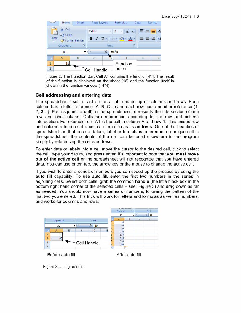
Immediately below the Ribbon is the Function Bar (or formula bar). The left portion of the function bar shows you what cells are currently active. In Figure 1 and Figure 2 the active cell is A1. The right part of the bar displays the contents of the cell, and more importantly, if a function has been entered the function is displayed. The cell within the spreadsheet normally shows the result of the function. In Figure 1 the cell A1 shows 16, while the function window shows the formula =4*4.

To see all formulas in the spreadsheet at once press control+.

Function bar

Cell (A1)

Worksheet tabs

Tabs Ribbon


Figure 2. The Function Bar. Cell A1 contains the function 4*4. The result of the function is displayed on the sheet (16) and the function itself is shown in the function window (=4*4).

Cell addressing and entering data The spreadsheet itself is laid out as a table made up of columns and rows. Each column has a letter reference (A, B, C…) and each row has a number reference (1, 2, 3…). Each square (a cell) in the spreadsheet represents the intersection of one row and one column. Cells are referenced according to the row and column intersection. For example: cell A1 is the cell in column A and row 1. This unique row and column reference of a cell is referred to as its address. One of the beauties of spreadsheets is that once a datum, label or formula is entered into a unique cell in the spreadsheet, the contents of the cell can be used elsewhere in the program simply by referencing the cell’s address.

To enter data or labels into a cell move the cursor to the desired cell, click to select the cell, type your datum, and press enter. It's important to note that you must move out of the active cell or the spreadsheet will not recognize that you have entered data. You can use enter, tab, the arrow key or the mouse to change the active cell.

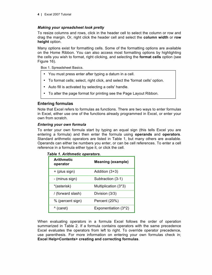
If you wish to enter a series of numbers you can speed up the process by using the auto fill capability. To use auto fill, enter the first two numbers in the series in adjoining cells. Select both cells, grab the common handle (the little black box in the bottom right hand corner of the selected cells – see Figure 3) and drag down as far as needed. You should now have a series of numbers, following the pattern of the first two you entered. This trick will work for letters and formulas as well as numbers, and works for columns and rows.

Before auto fill After auto fill

Cell Handle

Cell Handle Function button

Figure 3. Using auto fill.


Making your spreadsheet look pretty To resize columns and rows, click in the header cell to select the column or row and drag the margin. Or, right click the header cell and select the column width or row height option.

Many options exist for formatting cells. Some of the formatting options are available on the Home Ribbon. You can also access most formatting options by highlighting the cells you wish to format, right clicking, and selecting the format cells option (see Figure 16).

Box 1. Spreadsheet Basics.

Entering formulas Note that Excel refers to formulas as functions. There are two ways to enter formulas in Excel, either use one of the functions already programmed in Excel, or enter your own from scratch.

Entering your own formula To enter your own formula start by typing an equal sign (this tells Excel you are entering a formula) and then enter the formula using operands and operators. Standard arithmetic operators are listed in Table 1, but many others are available. Operands can either be numbers you enter, or can be cell references. To enter a cell reference in a formula either type it, or click the cell.

Table 1. Arithmetic operators. Arithmetic operator Meaning (example)

+ (plus sign) Addition (3+3)

- (minus sign) Subtraction (3-1)

*(asterisk) Multiplication (3*3)

/ (forward slash) Division (3/3)

% (percent sign) Percent (20%)

^ (caret) Exponentiation (3^2)

When evaluating operators in a formula Excel follows the order of operation summarized in Table 2. If a formula contains operators with the same precedence Excel evaluates the operators from left to right. To override operator precedence, use parenthesis. For more information on entering your own formulas check in; Excel Help>Contents> creating and correcting formulas.

• You must press enter after typing a datum in a cell.

• To format cells; select, right click, and select the 'format cells' option.

• Auto fill is activated by selecting a cells' handle.

• To alter the page format for printing see the Page Layout Ribbon.


Table 2. Operator precedence in Excel. Precedence Operator Description

1 : (colon) (single space) , (comma)

Reference operators

2 – Negation (as in –1) 3 % Percent 4 ^ Exponentiation 5 * and / Multiplication and division 6 + and – Addition and subtraction

7 & Connects two strings of text (concatenation)

8 = < > <= >= <> Comparison

Using Excel's functions The easiest way to understand the implementation of Excel functions is by following a step by step example.

There are three ways to access Excel's functions, click the function button next to the function window (a popup window appears), find the function on the Formulas Ribbon, or type = followed by the function name and a bracket {e.g. =sum( }.

In this first example we will calculate the sum of a series of numbers.

Figure 4. Excel's Auto Sum.

Step 1. Start by entering the series of numbers as pictured in Figure 4. Place your cursor in cell A7. Click the AutoSum button on the Formulas Ribbon. Excel tries to guess the cells you wish to sum up. Generally it will select all the cells containing numerical data immediately next to the cell you are inserting the function into. Notice that the cells Excel has chosen to sum are surrounded by a marching box (and the range is displayed in the Function Bar).


Figure 5. Excel's sum function.

Step 2. You can always override Excel’s selection by selecting the cells yourself, or typing the correct range in the Function Bar. Hit enter to see the resulting sum. The sum will appear in the cell where the function was entered. Note that when you select cell A7, the function appears in the function window, but the result will still appear in the cell on the spreadsheet.

In this second example, we will calculate the standard deviation for the same numbers used in the sum example.

Figure 6. Excel's Insert Function window.

Step 1. Place your cursor in cell A8. Select Formulas > Insert Function. Step 2. The Insert Function window appears. Here you can either search for the function by name, or select a category, and then scroll down looking for the function. Notice the description of the selected function appears near the bottom of the window. Enter 'standard deviation' in the search window and click 'Go'. Select the function STDEV and click ‘Ok’.

Figure 7. Excel's Function Arguments window.

Step 3. The 'Function Arguments' window now appears. You can either enter the cell addresses manually or select the cells on the spreadsheet. Notice Excel has chosen A1 to A7 but A7 I is the sum so we don’t want that included.


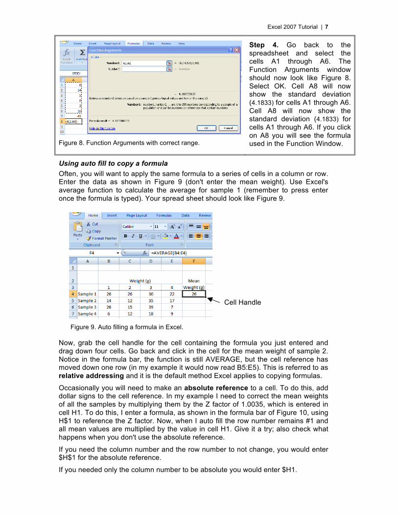
Figure 8. Function Arguments with correct range.

Step 4. Go back to the spreadsheet and select the cells A1 through A6. The Function Arguments window should now look like Figure 8. Select OK. Cell A8 will now show the standard deviation (4.1833) for cells A1 through A6. Cell A8 will now show the standard deviation (4.1833) for cells A1 through A6. If you click on A8 you will see the formula used in the Function Window.

Using auto fill to copy a formula Often, you will want to apply the same formula to a series of cells in a column or row. Enter the data as shown in Figure 9 (don't enter the mean weight). Use Excel's average function to calculate the average for sample 1 (remember to press enter once the formula is typed). Your spread sheet should look like Figure 9.

Figure 9. Auto filling a formula in Excel.

Now, grab the cell handle for the cell containing the formula you just entered and drag down four cells. Go back and click in the cell for the mean weight of sample 2. Notice in the formula bar, the function is still AVERAGE, but the cell reference has moved down one row (in my example it would now read B5:E5). This is referred to as relative addressing and it is the default method Excel applies to copying formulas.

Occasionally you will need to make an absolute reference to a cell. To do this, add dollar signs to the cell reference. In my example I need to correct the mean weights of all the samples by multiplying them by the Z factor of 1.0035, which is entered in cell H1. To do this, I enter a formula, as shown in the formula bar of Figure 10, using H$1 to reference the Z factor. Now, when I auto fill the row number remains #1 and all mean values are multiplied by the value in cell H1. Give it a try; also check what happens when you don't use the absolute reference.

If you need the column number and the row number to not change, you would enter $H$1 for the absolute reference.

If you needed only the column number to be absolute you would enter $H1.

Cell Handle


Figure 10. Using an absolute reference in Excel.

Box 2. Entering formulas.

• All formulas start with an = sign. • Case is not important when entering the formula. • Cells containing non numerical entrees will be ignored in calculations. • Excel functions are listed in; Excel Help>Contents>Function Reference. • The default for auto filling formulas is to use relative addressing.


Graphing The following example will show you how to make a scatter plot, add a linear regression trend line, and how to fine tune the graphs appearance.

Making a scatter plot

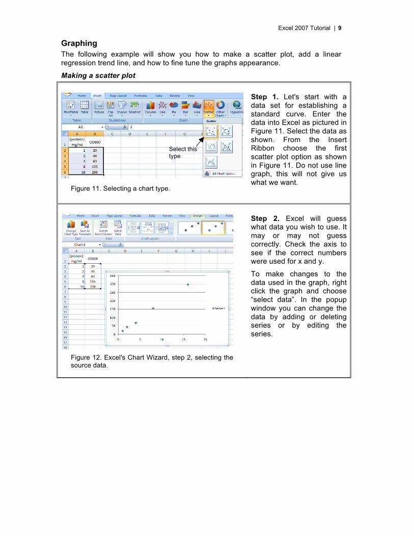
Figure 11. Selecting a chart type.

Step 1. Let's start with a data set for establishing a standard curve. Enter the data into Excel as pictured in Figure 11. Select the data as shown. From the Insert Ribbon choose the first scatter plot option as shown in Figure 11. Do not use line graph, this will not give us what we want.

Figure 12. Excel's Chart Wizard, step 2, selecting the source data.

Step 2. Excel will guess what data you wish to use. It may or may not guess correctly. Check the axis to see if the correct numbers were used for x and y.

To make changes to the data used in the graph, right click the graph and choose “select data”. In the popup window you can change the data by adding or deleting series or by editing the series.

Select this type


Figure 13. Excel's Chart Wizard, step 2, selecting the source data.

To check the X values click the small box containing the red arrow next to the X value window. This button takes you back to the spreadsheet. The data being used as X values will be in a marching dash box. To change the data being used, just re-select it. Similarly, check the Y data.

Remember, your X axis is always the controlled variable (in this case the protein concentration).

This button appears in many Excel source data windows, clicking it will always take you back to the spreadsheet, allowing you to select cells for input.

Clicking this button will take you back to source data window you started from.

Step 3. To add axis titles and change the chart formatting, select the chart and go to the Layout Ribbon. The buttons are pretty much self explanatory. Here I added an Axis Titles and a Chart Title, removed the series title (not needed if only one series), and the Gridlines (Figure 14).

Figure 14. Modifying the chart layout.

Excel 2007 Tutorial |11

Step 4. As this is a standard curve that will be used to estimate protein concentrations from OD600 readings I also did a regression analysis. Under Trendline I selected ‘linear trendline’ and under Trendline > More Trendline Options, I selected ‘Display Equation on chart’ and ‘Display R-squared value on chart’ (Figure 15).

Figure 15. Trendline options.

Box 3. Graphing basics.

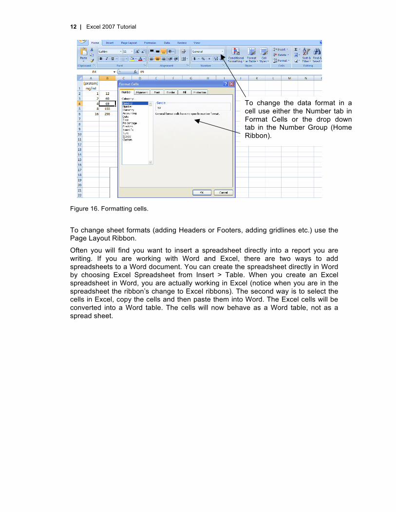
Formatting Spreadsheets Most formatting can be done from the Home Ribbon, or by right clicking a cell(s) and selecting ‘Format Cells’. The Format Cells window has several tabs that control most cell features (see Figure 16). For example, under the Number tab you can select a variety of formats for the cell contents. If you format the cell contents as Number, you can set the number of decimal places (Excel will automatically round the number for you). Once you have formatted a cell as a number, any non-number characters are ignored by Excel when the data is sorted.

• Once your graph is made it will automatically be updated to reflect any changes you make to the data used to create the graph.

• To modify most things on your graph use the Layout Ribbon.

• To modify the chart layout, the chart must be selected.

• The default formatting offered by Excel is rarely appropriate for science applications.


To change sheet formats (adding Headers or Footers, adding gridlines etc.) use the Page Layout Ribbon.

Often you will find you want to insert a spreadsheet directly into a report you are writing. If you are working with Word and Excel, there are two ways to add spreadsheets to a Word document. You can create the spreadsheet directly in Word by choosing Excel Spreadsheet from Insert > Table. When you create an Excel spreadsheet in Word, you are actually working in Excel (notice when you are in the spreadsheet the ribbon’s change to Excel ribbons). The second way is to select the cells in Excel, copy the cells and then paste them into Word. The Excel cells will be converted into a Word table. The cells will now behave as a Word table, not as a spread sheet.

To change the data format in a cell use either the Number tab in Format Cells or the drop down tab in the Number Group (Home Ribbon).

Figure 16. Formatting cells.

lauri's excel 2007 tutorial -...

Documents