layers in a raster model

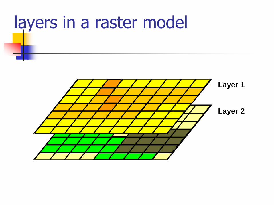
layers in a raster model

Layer 1

Layer 2

layers in an vector-based model (1)

Layer 2

Layer 1

layers in an vector-based model (2)

raster versus vector data model

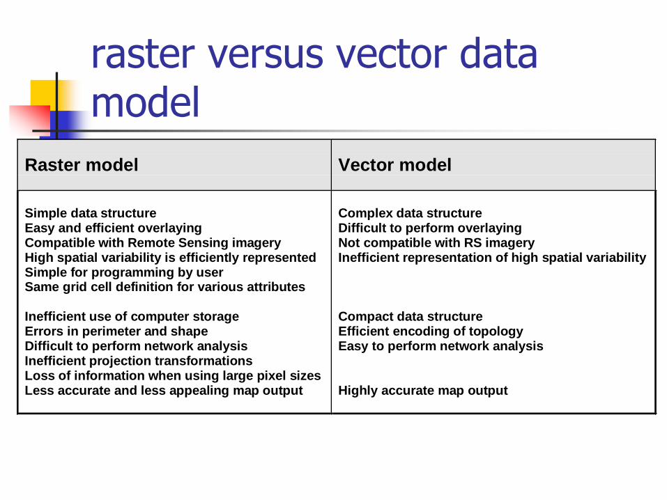
Raster model Vector model

Simple data structureEasy and efficient overlayingCompatible with Remote Sensing imageryHigh spatial variability is efficiently representedSimple for programming by userSame grid cell definition for various attributes

Inefficient use of computer storageErrors in perimeter and shapeDifficult to perform network analysisInefficient projection transformationsLoss of information when using large pixel sizesLess accurate and less appealing map output

Complex data structureDifficult to perform overlayingNot compatible with RS imageryInefficient representation of high spatial variability

Compact data structureEfficient encoding of topologyEasy to perform network analysis

Highly accurate map output

Quadtree data structure

In this, geographical area is decomposed into four quadrants and the decomposition continues until each quad represents a homogenous unit. The storage requirement of a quadree is much lower than that of a raster having the resolution of the smallest quad element

Quadtree data structure

In this, geographical area is decomposed into four quadrants and the decomposition continues until each quad represents a homogenous unit. The storage requirement of a quadtree is much lower than that of a raster having the resolution of the smallest quad element

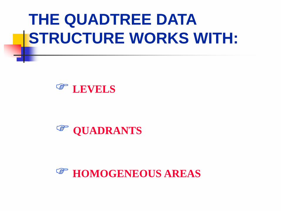
THE QUADTREE DATA

STRUCTURE WORKS WITH:

LEVELS

QUADRANTS

HOMOGENEOUS AREAS

Quad trees

advantages : - computation of standard region

properties is easy

- variable resolution and hence

less storage requirement

disadvantages : - translation invariant (two regions

having same size and shape can produce different

quadtrees.

- cannot split into parts

Course Content Introduction to GIS, Definitions of GIS and Overview,

History and concepts of GIS, Development of GIS, Scope and application areas

Geographical Entities, Attribute data, Linking spatial and attribute data

Spatial Data Models, raster vs vector, Raster data Models, Spatial Relationships, GIS Data Analysis, Raster data analysis tools

Mapping concepts, Map elements, Map scales and representation, Map projections and coordinate systems

Practical and Case Studies

Laboratory Sessions: Introduction to Arc GIS, Strength of Arc GIS, Some hands-on session in introducing the ARC GIS environment

Feature relationships & Topology

There are vast number of possible relationships in

spatial data.

Relationships are important in GIS analysis.

"is contained in" relationship between a point and an area is

important in relating objects to their surrounding environment.

"intersects" between two lines is important in analyzing

routes through networks

Relationships can exist between entities of the same

type or of different types.

for each shopping center, can find the nearest shopping center

(same type)

for each customer, can find the nearest shopping center

(different types)

Types of relationship

Relationships which are used to construct complex objects from simple

primitives.

Relationship between a line and the ordered set of points which

defines it.

Relationship between a polygon and the ordered set of lines which

defines it.

Relationships which can be computed from the coordinates of the

objects .

Areas can be examined to see which one encloses a given point -

the "is contained in" relationship can be computed.

Areas can be examined to see if they overlap - the "overlaps"

relationship.

Relationships which cannot be computed from coordinates

We can compute if two lines cross, but not if the highways they

represent intersect (may be an overpass).

Objects representing "house", "lot", “plot", with associated

attributes might be grouped together logically as “sellers account“.

Spatial relationships

Point-point

"is within", e.g. find all of the customer points within 1 km of

this retail store point

"is nearest to", e.g. find the hazardous waste site which is

nearest to this groundwater well

Point-line

"ends at", e.g. find the intersection at the end of this street

"is nearest to", e.g. find the road nearest to this aircraft crash

site

Point-area

"is contained in", e.g. find all of the customers located in this

ZIP code boundary

"can be seen from", e.g. determine if any of this lake can be

seen from this viewpoint

Spatial relationships

Line-line

"crosses", e.g. determine if this road crosses this river

"comes within", e.g. find all of the roads which come within 1

km of this railroad

"flows into", e.g. find out if this stream flows into this river

Line-area

"crosses", e.g. find all of the soil types crossed by this railroad

"borders", e.g. find out if this road forms part of the boundary

of this airfield

Area-area

"overlaps", e.g. identify all overlaps between types of soil on

this map and types of land use on this other map

"is nearest to", e.g. find the nearest lake to this forest fire

"is adjacent to", e.g. find out if these two areas share a

common boundary

Relationships as attributes

Example: “Flows-in” relationship

Option A Option B

Link ID Downstream

001 004

002 004

003 005

004 005

005 empty

001

003 004

002

005

Each stream link in a stream network could be given the

ID of the downstream link which it flows into

Flow could be traced from link to link by

following pointers

0001

0002 Link ID Pointer

001 0001

002 0001

003 0002

004 0002

005 empty

Point ID Pointer

0001 004

0002 005

Each stream link in a stream network could be

given the ID of the downstream point which

it flows into Each stream point in a stream

network could be given the ID of the

downstream link which it flows into Flow

could be traced from link to link by

following pointers

Relationships as attributes

Example: “is contained in” relationship

Well ID County

001 A

002 B

003 A

004 A

County ID No. of Wells

A 3

B 1

County A County B

001 002

003 004

1. Find the containing

county of each well

(compute the “is

contained in”

relationship).

2. Store the result as a new

attribute, County, of each

well.

3. Using this revised

attribute table, total flow

by county and add results

to the county table.

Object Pairs

Some attribute is between a pair of objects.

Distance is the attribute of a pair of objects.

Flow of commuters between two places.

Trade between two counties.

In some cases these attributes can be attached to an

object linking the origin and destination objects.

For example, trade can be attached to an arrow

pointing from county A to B.

In general, these kind of attributes shall be described

using separate tables or matrix.

A B C D

A 0 1 1.5 2.5

B 1 0 1 2

C 1.5 1 0 3

D 2.5 2 2.5 0

A distance table between

points A, B, C, and D

A B

C

D

Topology

Topology is a branch of mathematics that deals with properties

of space that remain invariant under certain transformations.

Properties : 3 spatial relationships

Containment: Polygons can be defined by set of lines enclose them

Contiguity: Identification of polygons which touch each other or

connect identify contiguous polygons (left or right)

Connectivity: Identification of interconnected arcs, starting point

& end point of network analysis

GIS topology

Topology is a mathematics approach that defines unchangeable

spatial relationships.

When a map is stretched or distorted, some properties change,

Distance

Angles

Relative proximities

Some properties won’t change,

Adjacencies

Most other relationships, such as "is contained in", "crosses"

Types of spatial objects - areas remain areas, lines remain lines,

points remain points

These unchanged properties are called topological properties.

Topological examples

Network connectivity Polygon adjacency

Topology well-defined

Topology poorly-defined

Importance of topology

Topology enables operations like connectivity and

contiguity analysis.

Searching a shortest path

Finding a service area by using a road network

Finding adjacent areas

Topology enables spatial analysis without using a

coordinate set,

Apply spatial analysis using topological definitions

alone

Major difference from CAD or computer-aided

cartography

Topology and GIS analysis

Searching a shortest path

The shortest path from the blue point to the yellow

point is through the red point and then the

orange point (2+1+2.5=5.5 map units).

However, if the topology of the red point is not

defined clearly, which means the two purple

lines are consider as one and the two orange

lines are considered as one, the resulting answer

will be wrong (2+2+2=6 map units).

Finding adjacent areas

The overlapped two polygons have to be

cut into three in order to clearly

defined the spatial topology.

Otherwise there will be difficulties

finding an adjacent polygon of either.

2.5

2 3

2.5

1

2

2

2

When editing features, it's important to maintain the spatial relationships that exist among them. For example, when you edit the shared boundary between two land use features, you don't want to introduce a gap between the two. To prevent editing errors, you can create a topology.

The spatial relationship between two polygon features is distorted when edited incorrectly.

Editing coincident features

The primary purpose of a topology is to define spatial relationships between features. The primary spatial relationships that you can model using topology are adjacency (contiguity), coincidence (containment) and connectivity.

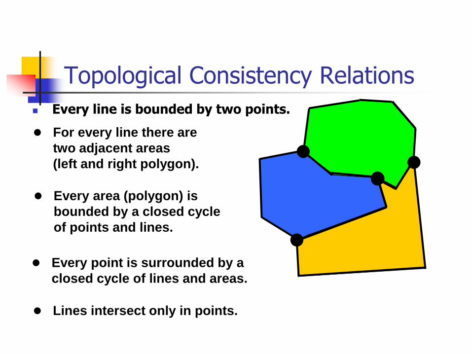
Topological Consistency Relations

Every line is bounded by two points.

For every line there are

two adjacent areas

(left and right polygon).

Every area (polygon) is

bounded by a closed cycle

of points and lines.

Every point is surrounded by a

closed cycle of lines and areas.

Lines intersect only in points.

Topological Invariants

Interior Boundary Exterior

Topological Relationships

Relationships between two regions can be determined based on the intersection of their boundaries and interiors (4-intersection).

A B

Lines: fundamental spatial data model

• Lines start and end at nodes

• line #1 goes from node #2 to node #1

• Vertices determine shape of line

• Nodes and vertices are stored as coordinate pairs

node

node

vertex

vertex

vertex

vertex

• Polygon #2 is bounded by lines 1 & 2

• Line 2 has polygon 1 on left and polygon 2 on right

Polygons: fundamental spatial data model

• complex data model, especially for larger data sets

• “arc-node topology,” used for ArcInfo data sets or defined by

rules in the Geodatabase.

Polygons: fundamental spatial data model

disjoint

meet

equal

inside

covered by

contains

covers

overlap

Spatial Relationships

Spatial Relationships Between Geometries – Boolean operators

Adjacency - Intersect

Coincidence - Touch

Connectivity- Disjointness

Equal – the same

Disjoint – contain a common point

Intersect – cut each other

Touch – at boundaries

Cross – overlap (different dimensions)

Within – is one within another

Contain – completely within another

Overlap (same dimension)

Relate – are intersections between the interior, boundary, or exterior of boundaries

Geometry and Features

Feature Geometry

Envelopes Polygons

Points and Multipoints Polylines

Geometry and Features

Components of Feature Geometries

Segments Paths

Rings

Attributes of Feature Geometries

Linear measurements with m values Vertical measurements with z values

Testing Spatial Relationships

Equals Contains


Within Crosses


Disjoint

Overlaps

Touches

Applying Topological Operators

Buffer

Clip

Convex

Hull

Cut

Applying Topological Operators

Difference

Intersect

Symmetric

Difference Union

Define an area where spotted owls have been spotted

Convex Hull

Create a convex hull for data set –the smallest convex polygon that contains the set of points

(Raster based) overlay operation tools

Arithmetic functions (+, - , * , /)

Relational functions (< , > , =)

Logical operations (and , or , xor , not)

Conditional functions ( if , then , else )

Logical functions

Boolean operators

AND =

OR

XOR

NOT

=

=

=

intersection

union

A

A

A

A

A B B

B

B

B

exclusion

negation

A

A

A

B

B

B

MapC= MapA + 10

15 12

16

15

15 15 15

12

12

121212

16 16 16 16

Map C

MapC1= MapA + MapB

9 10

7

9

9 9 9

10

10

1033

7 7 14 14

Map C1

4 84

4 4 4

8

8

81

1 1

1

8 8

1

Map B

5

5 5 5

5 2 2

2

2226

6 6 6 6

Map A

MapC2= ((MapA - MapB)/(MapA + MapB)) *100

11 60

71 3333

71 71 14 14

11

111111

60

60

60

Map C2

Arithmetic operations

-

- - -

- -

Relational functions

Output = MAP A > MAP B

4 84

4 4 4

8

8

81

1 1

1

8 8

1

Map B

5

5 5 5

5 2 2

2

2226

6 6 6 6

Map A

1

0

0

0

0

0

0

1

1

1 1 1

11

1 1

Output

0 = FALSE

1 = TRUE

Relational and logical operators

F = forest7 = 700 m6 = 600 m4 = 400 m

0

0 0 0 0 0

0000

0

0

0 0 0 0 0

0

0

1 1 1

111

Map D

MapD=(MapA= “Forest”) and (MapB <500)

0

00

0000

0

111

1 1

1 1

11

11

1

1 1

1

1

1

1

Map D1

MapD1=(MapA= “Forest”) or (MapB <500)

01

00

0

0

000

0 0 0 0

00

1 1 1

1

1

1 1

11

1

Map D2MapD2=(MapA= “Forest”) xor (MapB <500)

1

0

1 1

11

11

0 0 0 0 0

0 0 0 0 0

0 0 0

0 0

0 0

Map D3MapD3=(MapA= “Forest”) and not (MapB <500)

7 7 7 7

7777

4

4

4

44

44

4

44

6 6

6 6 6 6 6

F F F

FF

F F

F

F

FF

F F

0 = false

1 = true

Conditional functions

?

111

1 1

1 1

11

1 1

1

1

Map C

?

?

?

? ?

?

?

?

?

?

?MapC= iff(MapA= “Forest”,1,?)

F F F

FF

F F

F

F

FF

F F

1

0

1 1

11

0 0 0 0 0

0 0 0 0 0

0 0 0

0 0

0 0

Map C1

0 0

MapC1= iff((MapA= “Forest”)

and (MapB= 700),1,0)7 7 7 7

7777

4

4

4

44

44

4

44

6 6

6 6 6 6 6

F = forest7 = 700 m6 = 600 m4 = 400 m

0 = false

1 = true

? = undefined

Overlaying using and statement

Landuse = forest Slope = steep AND

layers in a raster model

Documents