layout-based substitution tree indexing and retrieval...

Layout-Based Substitution Tree Indexing and Retrieval for

Mathematical Expressions

APPROVED BY

SUPERVISING COMMITTEE:

Richard Zanibbi, Chair

Bo Yuan, Reader

Paul Tymann, Observer



by

Matthew Thomas Schellenberg

THESIS

Presented to the Faculty of the Golisano College of Computer and Information Sciences

Rochester Institute of Technology

in Partial Fulfillment

of the Requirements

for the Degree of

Master of Science, Computer Science

Rochester Institute of Technology

November 2011

Acknowledgments

Thanks to my committee members for their insightful guidance and extraordinary

patience. Thanks to my experiment participants for their timely assistance. And thanks to

everyone who supported me throughout this remarkable journey.

iii

Abstract



Matthew Thomas Schellenberg

Rochester Institute of Technology, 2011

Supervisors: Richard Zanibbi

We introduce a new system for layout-based indexing and retrieval of mathemat-

ical expressions using substitution trees. Substitution trees can efficiently store and find

hierarchically-structured data based on similarity. Previously Kolhase and Sucan applied

substitution trees to indexing mathematical expressions in operator tree representation (Con-

tent MathML) and query-by-expression retrieval. In this investigation, we use substitution

trees to index mathematical expressions in symbol layout tree representation (LATEX) to

group expressions based on the similarity of their symbols, symbol layout, sub-expressions

and size.

We describe our novel substitution tree indexing and retrieval algorithms and our

many significant contributions to the behavior of these algorithms, including: allowing sub-

stitution trees to index and retrieve layout-based mathematical expressions instead of pred-

icates; introducing a bias in the insertion function that helps group expressions in the index

iv

based on similarity in baseline size; modifying the search function to find expressions that

are not identical yet still structurally similar to a search query; and ranking search results

based on their similarity in symbols and symbol layout to the search query.

We provide an experiment testing our system against the term frequency-inverse doc-

ument frequency (TF-IDF) keyword-based system of Zanibbi and Yuan and demonstrate

that: in many cases, the two systems are comparable; our system excelled at finding ex-

pressions identical to the search query and expressions containing relevant sub-expressions;

and our system experiences some limitations due to the insertion bias and the presence

of LATEX formatting in expressions. Future work includes: designing a different insertion

bias that improves the quality of search results; modifying the behavior of the search and

ranking functions; and extending the scope of the system so that it can index websites or

non-LATEX expressions (such as MathML or images).

Overall, we present a promising first attempt at layout-based substitution tree index-

ing and retrieval for mathematical expressions.

v

Table of Contents

Acknowledgments iii

Abstract iv

List of Tables viii

List of Figures ix

Chapter 1. Introduction 1

1.1 Problem Description . . . . . . . . . . . . . . . . . . . . . . . . . . . . . . . 2

1.2 Importance of Research . . . . . . . . . . . . . . . . . . . . . . . . . . . . . . 4

1.3 Assumptions and Limitations . . . . . . . . . . . . . . . . . . . . . . . . . . . 4

1.4 Our Contributions . . . . . . . . . . . . . . . . . . . . . . . . . . . . . . . . . 5

1.5 Thesis Outline . . . . . . . . . . . . . . . . . . . . . . . . . . . . . . . . . . . 6

Chapter 2. Background 8

2.1 Related Work . . . . . . . . . . . . . . . . . . . . . . . . . . . . . . . . . . . 8

2.2 Other MIR Systems . . . . . . . . . . . . . . . . . . . . . . . . . . . . . . . . 11

2.2.1 Math WebSearch . . . . . . . . . . . . . . . . . . . . . . . . . . . . . . 12

2.2.2 Keyword-Based Retrieval using Lucene . . . . . . . . . . . . . . . . . . 13

2.3 Graf’s Substitution Trees . . . . . . . . . . . . . . . . . . . . . . . . . . . . . 13

2.4 Our Substitution Trees . . . . . . . . . . . . . . . . . . . . . . . . . . . . . . 14

2.4.1 Definitions . . . . . . . . . . . . . . . . . . . . . . . . . . . . . . . . . 15

2.4.2 Indexing Expressions using Substitution Trees . . . . . . . . . . . . . . 18

2.4.3 Retrieving Expressions from Substitution Trees . . . . . . . . . . . . . 20

Chapter 3. Methodology 21

3.1 Summary of Algorithm Modifications . . . . . . . . . . . . . . . . . . . . . . 21

3.1.1 Predicates and Mathematical Expressions . . . . . . . . . . . . . . . . 21

3.1.2 The Insertion Bias . . . . . . . . . . . . . . . . . . . . . . . . . . . . . 22

3.1.3 Finding Relevant Results through Multiple Searches . . . . . . . . . . 24

vi

3.2 The Data Structures . . . . . . . . . . . . . . . . . . . . . . . . . . . . . . . 24

3.3 Implementing Basic Functions . . . . . . . . . . . . . . . . . . . . . . . . . . 25

3.4 The Indexing Algorithm . . . . . . . . . . . . . . . . . . . . . . . . . . . . . 27

3.4.1 Normalization of Mathematical Variables in Expressions . . . . . . . . 28

3.4.2 Looking for Matching Expressions . . . . . . . . . . . . . . . . . . . . 29

3.4.3 Finding the Most Common Specific Generalization for Substitutions . 35

3.4.4 Selecting the Best Branch for Insertion . . . . . . . . . . . . . . . . . . 38

3.4.5 The Insertion Function . . . . . . . . . . . . . . . . . . . . . . . . . . 41

3.5 The Retrieval Algorithm . . . . . . . . . . . . . . . . . . . . . . . . . . . . . 44

3.5.1 Unification: Matching on Both Sides . . . . . . . . . . . . . . . . . . . 45

3.5.2 Ranking Search Results . . . . . . . . . . . . . . . . . . . . . . . . . . 46

3.5.3 Creating Extended Variations of the Search Query . . . . . . . . . . . 47

3.5.4 A Detailed Description of the Retrieval Algorithm . . . . . . . . . . . 47

3.5.5 The Retrieval Algorithm: A More Elegant Solution . . . . . . . . . . . 51

3.5.6 A Detailed Description of the Ranking Algorithm . . . . . . . . . . . . 51

3.6 Summary . . . . . . . . . . . . . . . . . . . . . . . . . . . . . . . . . . . . . . 55

Chapter 4. Results and Discussion 56

4.1 Experiment and Results . . . . . . . . . . . . . . . . . . . . . . . . . . . . . 56

4.2 Discussion . . . . . . . . . . . . . . . . . . . . . . . . . . . . . . . . . . . . . 60

4.2.1 The Effects of LATEX Formatting . . . . . . . . . . . . . . . . . . . . . 61

4.2.2 The Shortcomings of the Insertion Bias . . . . . . . . . . . . . . . . . 63

4.3 Summary . . . . . . . . . . . . . . . . . . . . . . . . . . . . . . . . . . . . . . 64

Chapter 5. Conclusion and Future Work 65

5.1 Conclusions and Future Work on the Insertion Bias . . . . . . . . . . . . . . 66

5.2 Future Work on Substitution Tree Indexing and Retrieval . . . . . . . . . . . 67

Chapter 6. Appendix 71

Bibliography 89

vii

List of Tables

3.1 Example of Matching . . . . . . . . . . . . . . . . . . . . . . . . . . . . . . . 34

3.2 Example of Finding the MSCG for SLTs . . . . . . . . . . . . . . . . . . . . 39

3.3 Examples of Generated Search Queries . . . . . . . . . . . . . . . . . . . . . 50

3.4 Examples of a Generalized Search Query . . . . . . . . . . . . . . . . . . . . 52

4.1 Overall Experiment Results . . . . . . . . . . . . . . . . . . . . . . . . . . . 57

4.2 Search Results for Query 4 . . . . . . . . . . . . . . . . . . . . . . . . . . . . 59

6.1 Full Experiment Results . . . . . . . . . . . . . . . . . . . . . . . . . . . . . 72

6.2 Unweighted Experiment Results . . . . . . . . . . . . . . . . . . . . . . . . . 73

6.3 The Search Queries . . . . . . . . . . . . . . . . . . . . . . . . . . . . . . . . 74





6.8 Search Results for Query 6, Part 1 . . . . . . . . . . . . . . . . . . . . . . . 79







6.15 Experiment Ratings Distribution . . . . . . . . . . . . . . . . . . . . . . . . 86

6.16 Experiment Ratings Distribution for Queries 1-5 . . . . . . . . . . . . . . . . 87

6.17 Experiment Ratings Distribution for Queries 6-10 . . . . . . . . . . . . . . . 88

viii

List of Figures

2.1 Symbol Layout Tree . . . . . . . . . . . . . . . . . . . . . . . . . . . . . . . 15

2.2 Substitution Tree . . . . . . . . . . . . . . . . . . . . . . . . . . . . . . . . . 18

2.3 Insertion into a Substitution Tree . . . . . . . . . . . . . . . . . . . . . . . . 19

3.1 Example Substitution Tree Index . . . . . . . . . . . . . . . . . . . . . . . . 23

3.2 Pseudo-code for Matching, Part 1 . . . . . . . . . . . . . . . . . . . . . . . . 31



3.5 Definition for the MSCG Algorithm . . . . . . . . . . . . . . . . . . . . . . . 36

3.6 Example of Finding the MSCG . . . . . . . . . . . . . . . . . . . . . . . . . 37

3.7 Definition for the select Function . . . . . . . . . . . . . . . . . . . . . . . 40

3.8 Example of Selecting the Next Branch for Insertion . . . . . . . . . . . . . . 41

3.9 Definition for the redundant Function . . . . . . . . . . . . . . . . . . . . . 42

3.10 Example of LATEX to Symbol Layout Tree Representation . . . . . . . . . . . 43

3.11 Definition for the insert Function . . . . . . . . . . . . . . . . . . . . . . . 45

3.12 The Ranking Algorithm . . . . . . . . . . . . . . . . . . . . . . . . . . . . . 53

3.13 Pseudo-code for Ranking Identity Vectors . . . . . . . . . . . . . . . . . . . 54

ix

Chapter 1

Introduction

While information retrieval is a well-explored field of research, mathematical infor-

mation retrieval (MIR) is far less developed. We present a new MIR system that uses sub-

stitution trees [7, 8] to index mathematical expressions from a database of LATEX documents

and retrieve relevant search results. The substitution tree data structure, originally created

for automated theorem proving, has not been used for MIR with layout-based expressions

such as those written in LATEX. This novel approach to MIR is comparable to existing MIR

systems and promises to be even more effective upon further refinement.

Conventional search engines remain ineffective in finding mathematical expressions

due, in part, to their inability to correctly handle special mathematical notation and sym-

bols [18]. Some have tried building search engines focusing on MIR to specifically address

these issues, with varying success [27]. Notably, Kohlhase and Sucan [14] made a search

engine using substitution trees indexing Content MathML (which represents mathematical

semantics – see operator trees in [27]) and they only provide a partial description of their

specific implementation of the algorithm. We chose to index LATEX because it is a much more

widely used and available source for mathematical information, though our system could be

modified to index other encodings. Their system, in contrast to ours, is intended for partial

queries (where some of the terms are unknown) and does not emphasize symbols and symbol

layout (allowing a varied number and ordering of terms in matching expressions through

the use of special attribute tags). Zanibbi and Yuan have created a keyword-based MIR

1

system using Lucene that they show to be effective [29]. It uses a vector-space approach to

store LATEX expressions and a term frequency-inverse document frequency (TF-IDF) model

to rank search results. We will be using their system in our tests for comparison and, unlike

Kohlhase and Sucan, provide an experiment rating the quality of search results returned by

the two systems.

1.1 Problem Description

The goal for this thesis is to design novel indexing and matching algorithms using

substitution trees [7, 8] for a mathematical information retrieval system. We aim to improve

retrieval effectiveness over existing search engines: the overall relevance of the documents

that are returned from a LATEX database as results of a particular search query given in

LATEX notation. We will use Zanibbi and Yuan’s keyword-based system for comparison [29],

examining different ways that information retrieval algorithms represent expressions for in-

dexing purposes and explore how their current vector-space indexing model can be enhanced

or changed. Specifically, we are going to investigate methods of finding other expressions

in the matching process relevant to the search query by identifying sub-expressions that

are present in both the document and the search query and by detecting if the query or

its sub-expressions are equivalent to other expressions through structural similarity. My

hypothesis is that, by using a substitution tree indexing model, the relevance of

search results for queries of LATEX mathematical expressions will be improved

over a keyword-based vector-space indexing model of Zanibbi and Yuan: since the

substitution tree’s unique structure depicts sub-expressions as sub-trees, it should allow for

easier searching of similar sub-expressions than the linear vector-space model by comparing

the sub-trees of the search query and the contents of each indexed expression.

2

Mathematical information retrieval is important for the same reason that all infor-

mation retrieval is important [27, 30]. Instead of first considering why someone would search

for a mathematical expression, instead consider why someone would search for a word or

phrase on a search engine like Google. The answer lies in a need for information (in the

form of webpages and documents) relevant to the search query. Since so much information

is available through digitalized documents and the Internet, parsing through that informa-

tion to find what is relevant to a specific word, phrase or expression is very important. A

person could be looking for not only definitions, exercises, theorems and other information

directly containing the expression, but also relationships between the expression and other

expressions and information (for example, linking a2 + b2 = c2 to “Pythagorean Theorem”

and d =√x2 + y2). A search could also find relevant expressions and information through

partial matches on the query and through similarities to the query in symbols and symbol

layout (for example, linking a2 + b2 = c2 to a2 + b2 and x2 + y2 = z2). Through searching,

a user can normally learn a great deal about any given subject; thus the need for a good

mathematical information retrieval system is to promote learning itself – which, in turn, will

lead to future mathematical and technological innovation.

Many search engines specifically constructed for handling mathematical expressions

already exist, including Math WebSearch [14], ActiveMath [16], Mathdex [19], Whelp [2],

and Springer LATEX Search. However, each has limitations. Zanibbi and Yuan have begun

working on a robust search engine for mathematical expressions in an attempt to overcome

some of these limitations [29, 27]. One such limitation is the difficulty in providing a proper

user interface for entering mathematical expressions as search queries. Another common

problem includes limited sources of information, restrictions on data based on file type or

formatting and the need to manually edit documents in order to highlight indexing terms.

They work to alleviate this problem by using a database of LATEX documents which provides

3

a standard notation for writing mathematical expressions and a significantly large collection

of available documents (e.g. through arXiv.org). Most importantly, existing search engines

are sometimes brittle due to ineffective information archival schemes due to poor choice

in indexing methods. This can be improved with the development of an effective indexing

technique for documents with mathematical information, and is what this thesis will examine.

1.2 Importance of Research

Mathematical information retrieval (MIR) is still a young area of research. This thesis

hopes not only to build upon prior work done in MIR, but also more thoroughly examine

the substitution tree indexing model. As large quantities of information become accessible

to more and more people around the world, the ability to effectively retrieve information

pertinent to the user will become imperative. Furthermore, this thesis will explore aspects

of information retrieval that are essential to all work related to the field: namely, the issue

of determining and understanding the relevancy of search results, and how to evaluate that

relevance (making what is normally a subjective task into a quantitative evaluation for the

purposes of scientific research and future comparison). Finally, important ideas for future

research in MIR will be presented.

1.3 Assumptions and Limitations

The scope of our work is to create a new search engine for mathematical expressions

(which we also call a “mathematical information retrieval (MIR) system”) using substitution

trees. This search engine will index expressions found in a database of LATEX docuemnts

(as opposed to, for example, scraping the Internet) and will therefore be limited to the

expressions found in that database. Since our focus is on using substitution tree indexing

4

and retrieval, the components of our search engine requiring user interaction will not be

designed for widespread commercial use; for example, queries are written in LATEX syntax.

Additionally, our search engine will not be streamlined to ensure that it is as time or memory-

efficient as possible; our research instead focuses on a proof-of-concept study of retrieval

results. Since we ignored expressions containing more than 100 symbols and assume that

each letter is an individual symbol, our search engine does not work well with theorems or

any expressions that contain many words or sentences. Our search engine is not capable of

making mathematically semantic equivalences (unlike Kohlhase and Sucan [14]); we look for

relevant search results based on similarity in symbols and symbol layout. This also means

that the ranking of our search results is based on their similarity of symbol and symbol layout

to the search query. The search engine makes some assumptions for its behavior during the

retrieval process – such as that variable symbols hold no special meaning and can be replaced

with one another to provide relevant (though not identical) search results (x = y + 1 is the

same as a = b+ 1) – that we believe is desirable for the majority of users; however, since the

relevancy of search results is subjective, we can’t guarantee that this behavior is well-suited

for all users.

1.4 Our Contributions

The research presented in this paper offers the following contributions to the field of

mathematical information retrieval:

• The modified substitution tree for layout-based mathematical expressions and the

adaptation of the symbol layout tree encoding to LATEX syntax.

• The novel substitution tree-based indexing algorithm for layout-based mathematical

expressions incorporating a bias in the insertion algorithm that helps group expressions

5

in the index based on similarity in baseline size.

• The novel substitution tree-based retrieval algorithm for layout-based mathematical

expressions which retrieves expressions that are not identical yet still structurally sim-

ilar to a search query and a ranking algorithm that sorts search results based on the

similarity of an expression’s symbols and symbol layout to the search query.

• An experiment comparing our substitution tree MIR system to a leading MIR system

and a with results that show the two systems to be comparable overall but suggest

that our system can be improved in future implementations.

We have also provided our source code available online here:

http://www.cs.rit.edu/ dprl

1.5 Thesis Outline

The chapters contained within this paper present the full extent of our research:

Chapter 2 – Background: Previous work in MIR that is related to our research, an in-

troduction to substitution trees including formal definitions, and a brief summary of

the original indexing and retrieval algorithms.

Chapter 3 – Methodology: Description of the substitution tree indexing and retrieval al-

gorithms (and all relevant functions), including formal definitions, pseudocode, textual

and visual examples and our specific changes to the original algorithms.

Chapter 4 – Experiment and Results: Our experiment comparing two MIR systems,

our presentation of its results, and our discussion analyzing those results.

6

Chapter 5 – Conclusion and Future Work: Our conclusions and ideas for future work

based upon our research.

Chapter 6 – Appendix: Tables containing more detailed information concerning the re-

sults of our experiment.

7

Chapter 2

Background

This chapter discusses previous work in the field of mathematical information retrieval

including other MIR systems. It also introduces and defines substitution trees and other

relevant terms as well as summarizing the substitution tree indexing and retrieval algorithms.

2.1 Related Work

Information retrieval is a thoroughly explored area of artificial intelligence [10, 22].

Search engines such as Google are able to quickly retrieve a plethora of relevant information

from documents and web pages on the World Wide Web based on a simple text query

given by the user. However, these conventional retrieval algorithms are ineffective when

search queries contain mathematical expressions [18]: expressions are hard to represent as

queries through a simple textual search interface due to the use of unusual symbols or

notations; different mathematical fields may have different meanings for certain symbols

or notations [11]; important mathematical symbols such as operators, decimals, parentheses

and other punctuation are often ignored or misinterpreted; extracting mathematical symbols

from sources in a search database can be difficult because of the different ways expressions

are represented (PDF, images, LATEX, and MathML, to name a few); and, partially due to

this fact, indexing sources containing mathematical information is challenging. Therefore

creating a specialized search engine for mathematical information, whose search queries are

mathematical expressions and the indexes of the search database are generated considering

8

mathematical language and notation, is preferred over adapting current conventional textual

search engines but could complement such engines.

Information retrieval itself has been previously well defined. Hiemstra describes three

parts of the information retrieval process: representing document content (indexing), repre-

sentation of the user’s information need (search query formulation), and the comparison of

the two representations (matching) [10]. This thesis will address the indexing and matching

processes in order to find a better way of indexing the documents in the database and match

relevant documents with the search query. The problem is not only constructing these two

algorithms, but ensuring that they work together to achieve maximum potential. Hiemstra

discusses various approaches to indexing for information retrieval systems, including the

vector-space model which is currently used in Zanibbi and Yuan’s search engine [29]. In

this approach, each indexed document is represented by a vector which contains each term

deemed important by the indexing algorithm. The search query is similarly represented by

its own vector whose components are associated with the given search terms. Matching is

done through a scoring algorithm which compares the components of the search vector with

each of the document vectors individually. This method is effective because it is inexpensive

and able to identify documents with matching terms. However, the simplicity of the model

also means it is linear in the vector used to represent an item (meaning that it can only make

matches based on shared symbols) and thus cannot identify relevant documents if they do

not contain a matching term.

Historically, the vector-space model has suffered from a key challenge of assigning

appropriate weights to vector components [10]. This was due to difficulties implementing

an effective the standard term frequency-inverse document frequency (TF-IDF) weighting

algorithm used by most textual search engines. Zanibbi and Yuan modified this strategy

9

by indexing on individual expressions instead of on entire documents. This term frequency-

inverse formula frequency (TF-IFF) method weighs the importance of different terms in all

expressions against the importance of terms within a particular expression and produces

more precise retrieval results. A similar strategy treating each expression as a separate

document will be enacted in this thesis.

Zhao et al. specifically discuss the design of information retrieval systems and their

ability to understand mathematical information in such a system [30]. They present three

types of search engines: those which are “math-unaware,” treating mathematical notation

merely as text and ignoring its importances; those which are “syntactically math-aware,”

recognizing the syntactical structure of mathematical expression and matching terms at the

syntactic level; and those which are “semantically math-aware,” evaluating not only the

syntactical structure of mathematical expressions but also the semantic meanings of those

expressions. By definition, semantically math-aware systems are capable of manipulating

expressions and resolving mathematical equivalence between them, including in cases where

they are syntactically different but semantically identical; however, this semantic understand-

ing of expressions would seem to occur on varying levels depending on the extent to which

the system could match equivalent expressions (more on equivalence in the next section).

Graf introduces the substitution tree indexing method [7, 8], originally developed to

perform term substitution for automated theorm proving. A substitution tree represents

any set of idempotent substitutions. The nodes of the tree are substitutions, and each

branch in the tree represents a binding chain for variables. The substitutions of a branch

from the root down to a leaf node are combined to yield an instance of the root node’s

substitution. Retrieval is based on a representation of substitutions as lists of variable-term

pairs and a backtracking algorithm that traverses through the tree searching for appropriate

10

substitutions. Overall, substitution trees have low memory requirements (since it stores

substitutions and not complete terms) and provide high search speed compared to other tree

indexing methods [7, 8]. Substitution tree indexing is itself a combination of the pre-existing

discrimination tree and abstraction tree indexing methods, offering the advantages of both

small size and better indexing performance.

2.2 Other MIR Systems

Researchers have been working on a variety of other MIR systems for over a decade;

however, many are now old or deprecated.

LATEX Search, found at latexsearch.com, is a service provided by Springer (source:

www.springer.com). According to the site, the system allows users to search “over 1 million

LATEX equations embedded in tens of thousands of articles from various disciplines.” Entering

a search query produces two separate lists of results – one for exact matches and another for

“similar” matches – and individual results display the LATEX source code for the matching

expression, its converted image, and links to the source document.

ActiveMath is a learning environment created by Libbrecht and Melis [16] that con-

tains semantically represented mathematical content. It indexes definitions, examples, exer-

cises, and other mathematical content from documents in the OpenMath library by encoding

them as sequences of semantic tokens using a custom syntax and storing them in a Lucene

index. The system retrieves content by converting the search query into a sequence of se-

mantic tokens (like it does during indexing) and comparing those tokens to entries found in

the index.

Whelp is a content based mathematical search engine introduced by Asperti et al. [2]

that allows users to search through a library of 40,000 theorems from the Coq proof assistant.

11

Theorems are indexed using a “logic-independent metadata model” by relating objects in

the theorem based on their position (where possible positions include hypothesis, conclusion

and proof, among others). Queries are entered using a custom syntax similar to TEXwhich

is then converted into metadata and compared to the entries in the index. Search results are

a list of references to the matching theorems’ locations in the Coq library.

The Mathdex search engine, built by Miner and Munavalli [19], is able to convert all

types of mathematical content available on the Web into XHTML+MathML in order to cre-

ate an extensive index of mathematical expressions. This system uses weighted mathematical

n-grams to emphasize similarity of symbols and sub-expressions between expressions.

Miller and Youssef’s NIST Digital Library of Mathematical Functions (DLMF) Project

uses LATEXML to translate LATEX into XHTML and MathML for expression indexing [18].

They augmented an existing textual search engine for expression retrieval by implementing a

keyword-based expression representation and developing a custom mathematical query lan-

guage resembling TEX. They also added a thesaurus in order to enumerate terms that are

related (such as semantic equivalences or names for famous expressions) which they claim

“will continue to evolve.”

For our investigation, two of these systems are especially important: Math Web-

Search, which uses substitution trees to index Content MathML; and a system designed by

Zanibbi and Yuan [29] to index LATEX.

2.2.1 Math WebSearch

Math WebSearch, developed by Kohlhase and Sucan [14], is the first MIR system to

index expressions written in Content MatML (contained in MathML and OpenMath) using

substitution trees. They only provide a partial description of their code, including rough

12

pseudocode for their insertion function. Search queries are entered as Content MathML and

can include generic terms that take advantage of the unique structure of the substitution

tree in order to match a larger number of expressions. We seek to build upon their work

with substitution tree indexing by applying it to layout-based mathematical equations in

LATEX documents.

2.2.2 Keyword-Based Retrieval using Lucene

Zanibbi and Yuan’s keyword-based Lucene MIR system [29] uses a vector-space model

to index expressions from a database of LATEX documents and ranks search results based on

a TF-IDF (term frequency-inverse document frequency) relevance measure. Due to its effec-

tiveness, its use of layout-based expressions and its different indexing and retrieval models, we

will be testing our novel substitution tree MIR system against this system in our experiment

(described in Chapter 4).

2.3 Graf’s Substitution Trees

Graf first introduced the substitution tree as a tool for automated theorem proving

[7, 8]. It provides an efficient and intuitive way for storing predicates and grouping them

based on similarity. These predicates are composed of terms – variables, functions (terms

that also contain a set of terms) and constants (functions whose set of terms is empty) – and

the similarity of two predicates is based upon the terms they share and the arrangement of

those terms.

In a substitution tree, each node represents a predicate; the leaf nodes represent

specific predicates that have been inserted into the tree, while the non-leaf nodes represent

predicates containing one or more generalized variables, known as substitution variables.

13

Each child node specializes its parent by replacing one or more of these substitution variables

with specific terms; these replacements are called substitutions and are contained within the

node. Thus the predicates in the substitution tree go from more abstract to more specific

through substitutions. Following a branch of the tree from root to leaf will produce a

predicate represented by the leaf node through the combined substitutions of every node

along the branch. This also means that every child node is an instance of its parent, requiring

only a substitution (or set of substitutions) to produce the child’s predicate from the parent’s,

and every parent node is a generalization of each of its children. The substitution tree

represents all of the inserted predicates simultaneously and each predicate can be produced

by following a specific branch.

2.4 Our Substitution Trees

Our implementation uses mathematical expressions instead of predicates; expressions

themselves are essentially sets of terms, where each term represents a symbol in the expres-

sion. This makes our conversion much easier: each node in our substitution trees represents

an expression instead of a predicate, but otherwise their behavior is much the same. Substitu-

tion variables still replace terms, and substitutions are still made from substitution variables

to terms; terms simply represent a wider variety of symbols that appear in mathematical

expressions, such as operators (+, ∗, etc.).

We use another type of tree, called a symbol layout tree (or SLT), to represent the

expressions within the nodes of the substitution tree. An SLT is an encoding for a math-

ematical expression that is constructed based on the spatial relationship of the symbols in

that expression. Each node of the SLT contains a term that represents a variable, constant,

symbol or function in an expression. Each node has at least four branches dependent on

14

x NEXT + NEXT y

BELOW

1

ABOV E

2

Figure 2.1: The symbol layout tree for x2 + y1. The “above” branch is also used for termsthat are superscript to another term (a caret in LATEX), and the “below” branch for termsthat are subscript (an underscore).

the node’s term: one representing the term(s) positioned spatially to the right of the term,

one representing the term(s) positioned spatially above or superscript to the term, one rep-

resenting the term(s) positioned spatially below or subscript to the term, and one or more

representing the sets of terms that are argument(s) to the term, if the term is a function: in

LATEX functions (e.g., \frac), these are positioned within sets of brackets .

Due to the similarity of our representation of mathematical expressions to the pred-

icates used in Graf’s original implementation, the overall behavior for the indexing and

retrieval algorithms remains the same and is described in this section. Changes we have

made for our specific implementation of Graf’s definitions for substitution trees as well as

explicit descriptions of our code are detailed in Chapter 3.

2.4.1 Definitions

A symbol layout tree is described by a 5-tuple (t, A,B, X1, ..., Xn, N) where t is a

term and A, B, X1, ..., Xn and N are SLTs. A is the SLT positioned spatially above or

superscript to t, B is the SLT positioned spatially below or subscript to t, X1, ..., Xn are

15

the SLTs that are arguments to t, and N is the SLT positioned spatially to the right of

t (the next node). We assume that a LATEX term cannot have another term both above

and superscript to it, or both below and subscript to it. No node’s term may equal ∅ (the

empty set) but any node itself may equal ∅. We use the notation (t) as shorthand for

SLTs that only contain a term, and (t, N) for SLTs that only contain a term and a next

branch: (t) = (t, ∅, ∅, ∅, ∅), (t, N) = (t, ∅, ∅, ∅, N). We use the terms “SLT” and “expression”

interchangeably. For example, x2 + 5 ∗ √y1 = (x, (2), ∅, ∅, (+, (5, (∗, (\sqrt, ∅, ∅,

(y, ∅, (1), ∅, ∅), ∅))))).

The sub-expressions of an expression are all of the SLTs contained within Above,

Below and Argument branches, as well as those within parentheses, brackets and braces.

Sub-expressions themselves are also expressions and can contain sub-expressions of their

own. For example, the sub-expressions of xx∗(y+1)n−1 are n− 1, x ∗ (y + 1) and y + 1.

A substitution σ = S1 → T1, ..., Sn → Tn,∀i Si ∈ V represents a replacement of

each SLT Si with the corresponding SLT Ti. V is the set of variable symbols : single-node

SLTs which will hereafter be represented by N , where N is an integer. We will use the

term “substitution” to refer to both a set of substitutions (σ) and a single substitution

(S → T ). When a substitution σ is applied to an SLT X, each instance of Si ∈ σ in X is

replaced with Ti ∀i. For example, if σ = 1 → x2 = (x, (2), ∅, ∅, ∅), 2 → 5 = (5) and

X = 1 + 2 = ( 1 , (+, ( 2 ))), apply(σ,X) = Xσ = (x, (2), ∅, ∅, (+, (5))) = x2 + 5.

The domain of a substitution is defined as DOM(σ) := x ∈ V|xσ 6= x. The

codomain of a substitution is defined as COD(σ) := xσ|x ∈ DOM(σ). The image of a

substitution is defined as IM(σ) := VAR(COD(σ)) where VAR(T ) is the set of all substitution

variables occurring in the SLT T . Thus the image of a substitution is the set of all substitution

variables occurring in the codomain of that substitution. For example, if σ = 1 →

16

5, 2 → 3 + 4 , then image(σ) = 3 , 4 . A restriction σ|U where U ⊆ V means that

DOM(σ|U) ⊆ U .

Two substitutions σ = S1 → T1, ..., Sn → Tn and τ = X1 → Y1, ..., Xn → Yn can

be composed, or added together, using the following formula:

compose(σ, τ) = στ = S1 → T1τ, ..., Sn → Tnτ ∪ Xi → Yi|Xi ∈ DOM(τ)\DOM(σ)

For example, if σ = z → f(x) and τ = x → a, y → c, στ = z → f(a), x →

a, y → c. Notice that the order in which two substitutions are composed makes a difference

because the substitutions in σ are applied to τ but not visa-versa.

A substitution tree represents a set of substitutions where each node is a substitution

and each branch is a set of idempotent substitutions. (A substitution σ = S1 → T1, ..., Sn →

Tn is idempotent if ∀i Si does not appear in Ti). Each branch in the tree represents a

binding chain for variables, and, for any node, the composition of all substitutions in the

branch from the root to that node produce an expression that is an instance of the root node’s

substitution. Thus any node itself can be said to contain an expression which is found by

composing the substitutions from the root to that node. Any mathematical expression may

be inserted into a substitution tree where it becomes represented by a new node if it’s not

already in the tree. This insertion may also change existing nodes in order to create the most

generalized set of substitutions for all expressions contained within the tree. The order in

which the expressions are inserted impacts the layout of the substitution tree. A substitution

tree node is described by a tuple (τ,Σ) where τ is the substitution represented by the node

and Σ is the set of child substitution tree nodes. Since every node represents an expression,

we sometimes use “node” as shorthand for “the expression that the node represents.”

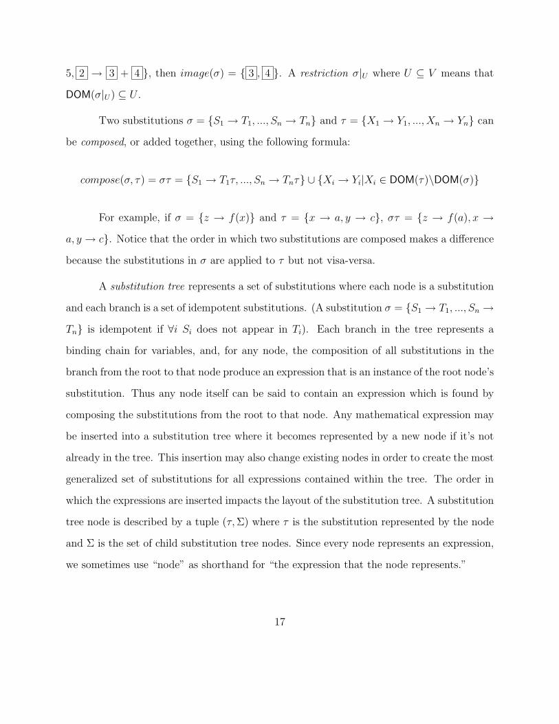
17

0 → 1 − 2

2 → 5

1 → 3 1 → ∗1

1 → 5, 2 → ∗1

Figure 2.2: A substitution tree representing the expressions x − 5, 3 − 5 and 5 − x. Theseexpressions are normalized to ∗1 − 5, 3 − 5, and 5 − ∗1 respectively. Indicator variables

can be substituted for any single mathematical variable; in this case, ∗1 → x. 0 is usedas the root substitution variable. An expression can be reconstructed by composing thesubstitutions along a branch. For example, the expression x − 5 is reconstructed using thefollowing set of substitutions: 0 → 1 − 2 , 2 → 5, 1 → ∗1 where ∗1 → x.

2.4.2 Indexing Expressions using Substitution Trees

Indexing mathematical expressions using substitution trees involves inserting all of

the expressions, one at a time, into a single substitution tree. This constructs a substitution

tree (the index ) that represents each expression.

Before a new expression is inserted into a substitution tree, all variables in the expres-

sion (hereafter known as mathematical variables) must be normalized by renaming them as

indicator variables, denoted by ∗i . An indicator variable is a type of substitution variable

that can only be substituted for a mathematical variable. Any indicator variable that is

not already bound can be substituted for any mathematical variable; so ∗i = a = . . . = z.

Variables are normalized in the order they appear in the input expression from left to right:

for example, x + y and y + x are both normalized to ∗1 + ∗2 . This normalization allows

a single node to represent multiple expressions, and this overlap helps both indexing (since

fewer nodes makes the tree smaller and insertion faster) and retrieval (since expressions with

such similarity should be relevant search results; after all, x can equal y in the right context).

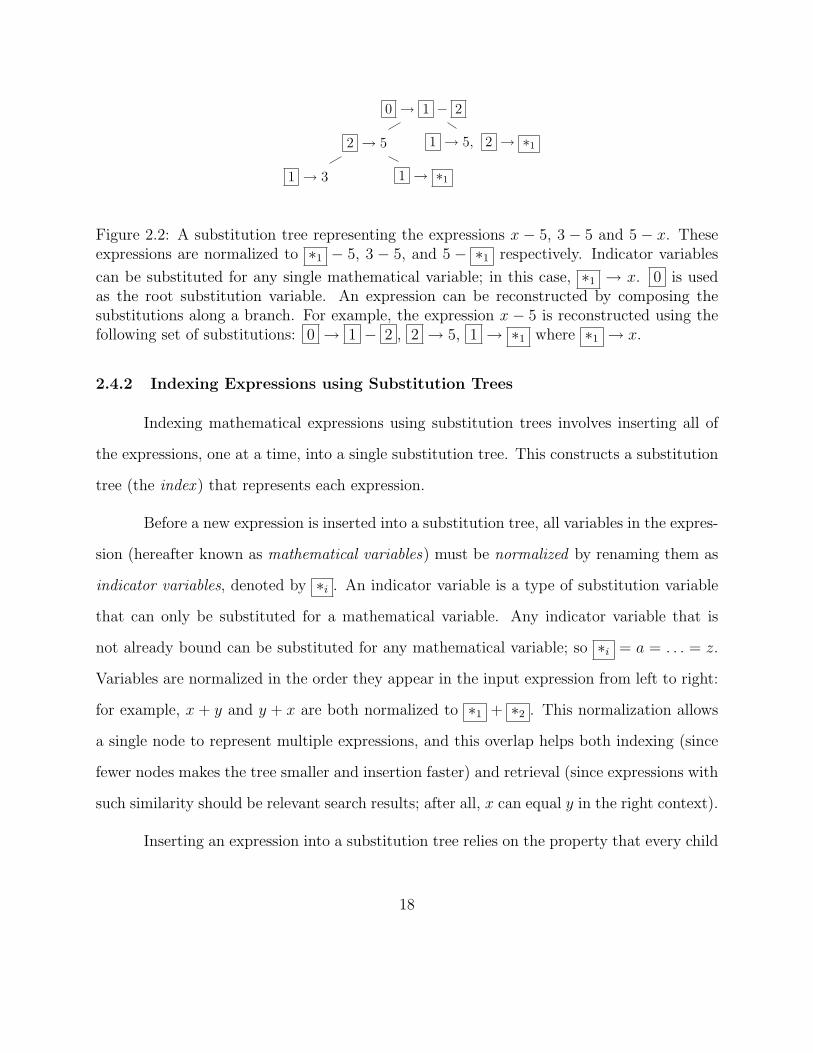
Inserting an expression into a substitution tree relies on the property that every child

18

0 → ∗1

0 → ∗11

1 → ∅ 1 → 2

∅

0 → ∗12 + ∗2

2

2 → ∅ 2 → 2

0 → ∗11

3

3 → ∅

1 → ∅ 1 → 2

1 → 2, 3 → 1

Figure 2.3: Top Left: The expression x is inserted into an empty substitution tree. Thetree now contains one node with a substitution from the root substitution variable 0 tothe normalized expression. This substitution will not only match x but also any singlemathematical variable. Bottom Left: Now x2 is inserted into the same substitution tree.Since no match could be found, it creates a generalization – a new node replacing the oldroot and its children. The two new children nodes represent more specifics instance of thisnew, generalized substitution. Right: The same substitution tree after the expressions x+y,x2 + y2 and x2

1 are added. A null substitution ∅ is sometimes produced if a generalizedsubstitution is empty. A substitution to ∅ represents a replacement of that substitutionvariable with nothing.

node is an instance of its parent and every parent node is a generalization of all its children.

The insertion algorithm takes a normalized expression e and first looks for a match among

the index root and its children. Two expressions match if one is an instance of another. If

any of the root’s children are a match, the algorithm is called recursively using that child as

the new root; if the root alone is a match, a new node representing e is created and added

to the root’s children. If none of the nodes are a match, then the algorithm finds the most

specific common generalization (MSCG) of e and the root, where the MSCG is a substitution

containing the most specific (the closest match) of all of the possible generalizations of the

two expressions. This generalization replaces the root node and takes two children of its

own: an instance of the root (and its original children) and an instance of e (a leaf node that

represent e). The MSCG algorithm is described in great detail in the next chapter.

19

2.4.3 Retrieving Expressions from Substitution Trees

Retrieving relevant mathematical expressions from substitution trees benefits from

the properties of the tree and the behavior of insertion. Finding exact matches to a search

query is straightforward because, if the expression exists in the index, it can be found by

simply following the correct branch (the branch that contains nodes that match the search

query). Expressions similar to the search query can be found while following the matching

branch due to the nature of how they were inserted. Since a new expression is inserted

into a branch that shares a common match or MSCG, that expression will share the most

similarities with its parent and siblings. These similarities are based on the expressions’

shared symbols and symbol layout (the arrangement of those symbols). Thus the parents

and siblings of a node that matches the search query will also be relevant search results.

The search algorithm works by seeing if the search query is a match to the index root.

If so, the algorithm is called recursively on each of the root’s children; if not, the search fails.

If the root is both a match and a leaf, the expression it represents is added to the list of

results.

An important note concerning the retrieval algorithm is that we in no way search

based on semantic relevancy. The search function cannot consider equivalences or mathe-

matical properties (such as 1+2 = 2+1), keyword associations (such as the names of famous

expressions) or other semantic knowledge.

20

Chapter 3

Methodology

The previous chapter explained the overall behavior of substitution tree indexing and

retrieval as it appeared in Graf’s original mathematical definitions for substitution trees

[7, 8]. This chapter introduces the necessary additions and modifications we’ve made to our

own substitution tree implementation in order to accommodate our innovative research in

indexing and retrieving mathematical expressions. We present these novel changes through-

out the chapter as we describe in great detail the different data structures and functions that

form our algorithms.

3.1 Summary of Algorithm Modifications

Some of the changes we’ve made are especially significant: the use of mathematical

expressions, the insertion bias, and the overall search behavior.

3.1.1 Predicates and Mathematical Expressions

As previously stated, we index whole mathematical expressions instead of predicates.

Expressions are more complex than predicates due to the spatial differences of their sym-

bols – superscript, subscript, above, below, or contained within a function. Additionally,

expressions are sets of terms rather than either being single terms or functions (which, while

similar, behave differently than sets of terms). We represent expressions in the index using

symbol layout trees (as discussed in the previous chapter), which is a layout-based encod-

21

ing for expressions. SLTs can be considered specialized 5-element predicates that can be

nested to form different branches of the tree depending on the symbol layout. Thanks to

the beauty of recursion, we can represent expressions using SLTs and still take advantage

of much of Graf’s substitution tree implementation. However, this change to SLTs required

modifying many of Graf’s functions for our own implementation – in particular, tracking the

corresponding branches of SLTs. Therefore we are specializing – rather than generalizing –

Graf’s representation and implementation.

Another change from Graf’s implementation is that our substitution variables can

have Above, Below, and Argument branches of its own, which can themselves also be substi-

tution variables. This was necessary because of our switch to SLTs and gives our substitutions

the ability to match a wider array of expressions through extended dimensionality.

3.1.2 The Insertion Bias

The most significant addition we made to the indexing algorithm was to introduce an

insertion bias. A bias is needed because otherwise most of the expressions group together in

a single branch from the index root. This is probably due to our transition from predicates to

expressions and the sheer size of our index. This behavior is not desired because it does not

take full advantage of the substitution tree’s structure and would make retrieval inefficient

(often forcing the algorithm to run an exhaustive search of the index). The bias we have

chosen is the size of the baseline, which is the set of SLT nodes starting from the root of

an expression and continuing along the Next branch of each node. The baseline size is not

affected by the number of non-empty Above, Below or Argument branches that extend from

the baseline nodes, nor their depth: thus x and xxyz both have a baseline size of 1, and x+ y

and cos x + 12

both have a baseline size of 3. An SLT node and its corresponding term are

said to lie along the baseline if it is part of this set. This bias is introduced in the match

22

∅. . .

Expressions ofbaseline size A

. . .

. . .Expressions ofbaseline size B

. . . . . .

Expressions ofbaseline size C

. . .

. . .

. . .

Figure 3.1: Essentially, the sub-trees of the substitution tree index’s root are separated bythe size of an expression’s baseline due to the baseline insertion bias.

and MSCG functions and causes each of the index root’s sub-trees to represent expressions

of a different baseline size. This specific bias is desirable because it helps group similar

expressions together (based on their size) which is useful for both indexing and retrieval

(since large expressions are less relevant to small search queries, and visa-versa).

While a single substitution variable can’t match multiple terms along the baseline

due to this bias, it can still match multiple terms that are above, below, or argument to the

terms along the baseline (in other words, non-baseline sub-expressions). For example, the

expression cos ( 1 ) can match cos (x+ 1) using the matcher 1 → x+ 1, but the expression

1 cannot match x+1 because it lies along the baseline. Additionally, a substitution variable

that does not lie along the baseline can match the empty substitution ∅, allowing us to match

expressions like x2 with x because x = x∅. This behavior is an inherent part of the algorithm

and is only superseded for nodes along the Next branch due to the baseline bias we have

implemented.

23

3.1.3 Finding Relevant Results through Multiple Searches

Graf’s search function takes an expression (the search query) and returns the expres-

sions in the index that are identical to the query. However, for our system, we want to find

both expressions that are identical to the query and also expressions that aren’t identical

but still relevant to the query. To solve this problem, for each search query entered by the

user, we make multiple searches using the query and variations on the query (including the

query’s sub-expressions [14]) generated by the retrieval algorithm. Kohlhase and Sucan’s

system do not search using additional queries but do include attributes to individual terms

in the query that allow them to match generic terms or an unspecified number or ordering

of terms. Our variations are described later in this chapter.

3.2 The Data Structures

SLTs are represented by a C struct containing an array of characters for the SLT’s

term, three pointers to other SLT structs for its Above, Below and Next branches (any of

which can be ∅ if that branch does not exist), and a vector of pointers to SLT structs for

its zero or more Argument branches. Substitutions are represented by C++ maps from

character pointers to SLT struct pointers. With a substitution σ = S1 → T1, . . . , Sn →

Tn, this map corresponds to each substitution Si → Ti where the character pointer is the

substitution variable (Si) and the SLT struct pointer is the expression (Ti). Substitution

trees are represented by a C struct containing a unique id (used for saving the tree to file),

a substitution map for the node’s set of substitutions, a vector of substitution tree pointers

for the node’s children, and two vectors – one of SLT struct pointers, another of character

pointers – for the node’s final expressions (as SLT structs) and the LATEX document within

which those expressions are contained. These last two vectors are always the same size, and

24

are always empty for non-leaf nodes and non-empty for leaf nodes. This information is saved

when an expression is first inserted into the substitution tree and is used when returning

search results.

Many of the functions in our system rely on either iterating recursively through nodes

in a tree (symbol layout or substitution) or through the elements in a substitution map.

Also, all functions that don’t return an integer are call-by-reference, so when we say that a

data structure is “returned” we really mean that it was given as a function argument and

thereafter modified. Functions that can succeed or fail return an integer (0 or 1) to designate

their outcome.

3.3 Implementing Basic Functions

All substitutions have basic inherent mathematical properties as described in the

previous chapter, including taking the domain or image of a substitution, applying a substi-

tution to an expression, and composing two substitutions. These functions are necessary for

the indexing and retrieval algorithms and their code implementations are described below.

The domain function takes a substitution map (a C++ map representing a substitu-

tion). It puts each of the map’s keys into a vector and returns that vector.

The image function is given a substitution map. For each element in the map, if that

element’s term is a substitution variable, the function puts that term into a vector. Then it

recurs on each of the element’s branches (calling itself on the Above node, Below node, Next

node, and each Argument node). The same vector is used for each element and each branch

and is returned by the function once all elements have been evaluated. The final vector

contains all of the substitution variables found in the codomain of the given substitution

map (the SLTs in each value of the map’s key-value pairs).

25

The apply function takes an SLT struct and a substitution map and returns a new

SLT struct. Starting at the SLT’s root (the “current node”), it looks for a key in the

substitution map that matches the current node’s term. If a matching key exists, we know

that the term is a substitution variable and that it has a known mapping in the input

substitution; therefore the function replaces the old term (in the current node) with the

new term (the term contained within the key’s corresponding SLT). The new term’s Next

branch is inserted into the SLT in front of the old term’s Next branch, and the new term’s

Above, Below and Argument branches, if non-empty, are copied over as well, completely

replacing those of the old term. This replacement can be done safely because the system is

designed to guarantee that a substitution variable with an Above, Below or Argument branch

will not be replaced by a term containing those branches (for example, the application of

the substitution 1 → x3 to the expression 12

will never exist in a substitution tree). The

function then recurs on each of the current node’s branches in order to apply the substitution

to the whole expression.

The compose function is given two substitution maps σ = S1 → T1, . . . , Sm → Tm

and τ = Q1 → R1, . . . , Qn → Rn and returns their composition as a new substitution

map. First, the function applies τ to each element in σ: Tiτ ∀i, 0 ≤ i ≤ m. The resulting

expression is added to the new substitution map with its corresponding key Si. Then each

substitution Qi → Ri where Qi ∈ DOM(τ)\DOM(σ) (for substitution variables Qi distinct

from S1, . . . , Sm) is added to the new substitution map as well (an example composition is

given in the previous chapter).

26

3.4 The Indexing Algorithm

The indexing process involves first taking a collection of LATEX documents and extract-

ing their mathematical expressions into individual files through Zanibbi and Yuan’s modified

version of the latex2html utility [29]. Each file is then converted from LATEX syntax to SLT

syntax by constructing a parse tree of the LATEX grammar and transforming the parse tree

into a linearized representation of SLTs using a custom TXL grammar [5]. These SLT files

are then inserted into the substitution tree index one after another. The order of insertion

is based on the name of the document and the order of appearance in that document. Once

the index has been created it is saved to a text file which allows the index to be recreated

when the program is run again.

It is important to note that, for the extraction process, mathematical expressions

written in “display mode” using double dollar signs ($$ ... $$) are treated exactly the same

as identical expressions written using single dollar signs ($ ... $) even though they might be

rendered with slightly different spacing. For example, generating the SLT for∑n

i=1 i always

puts the i = 1 in the Below branch even though it is shown as superscript to the summation

sign when using single dollar signs and below the summation sign when using double dollar

signs. Additionally, LATEX functions that show arguments as spatially above or below (such

as \frac) are treated like all other LATEX functions. For example, generating the SLT for 12

would create an SLT node containing \frac with empty Above, Below and Next branches

and two Argument branches containing 1 and 2 respectively.

This algorithm has a few shortcomings. First, it cannot consider semantic similarities

when inserting an expression, so, for example, 1 + 2 will not be matched to 2 + 1. Also, the

comparison of expressions during matching does not find the largest common subsequence of

the two expressions, but instead always starts comparing from the root of the SLT; therefore

27

2 + 1 and 3 + 2 + 1 will not be matched either. However, these expressions will likely still

be returned as relevant results during the retrieval process as described below. (Remember

that two expressions only match if one is an instance of another, and otherwise will not be

matched even if the two expressions are similar.)

The indexing algorithm contains five major parts: normalizing mathematical variables

in expressions, looking for matching expressions, finding the most specific common general-

ization of expressions, selecting branches in the tree for insertion, and inserting expressions

into the tree. The rest of this section describes each of these parts and their corresponding

functions.

3.4.1 Normalization of Mathematical Variables in Expressions

The arguments for the normalization function are an integer used to create new

indicator variables and two pointers to the root of an SLT: one will remain pointing to the

root, and the other will be advanced as the function iterates through the SLT (the “current

node”). It checks if the term contained in the current node needs to be normalized. If so, it

creates a new indicator variable using the input integer (and increasing it by one for future

use) to replace that term and iterates through the entire expression (from the root to the leaf

of each of its branches) replacing each instance of the term with the indicator variable. After

this check is completed, the function calls itself recursively on each of the current node’s

branches to ensure that the expression is fully normalized.

For normalization, we assume that mathematical variables are only represented by

single alphabetical characters (a, . . . , z) or greek characters (α, . . . , ω and A, . . . ,Ω). We also

assume an implied multiplication of consecutive alphabetical characters, so abc = a× b×c =

∗1 × ∗2 × ∗3 . Finally, we assume that all functions are preceded by a backslash, in

28

adherence to LATEX syntax, and are treated as a single term; thus \cosx will be treated as

a function while cosx will be treated as c× o× s× (x).

3.4.2 Looking for Matching Expressions

Comparing two expressions to determine if they have similarities in symbols or symbol

layout is done through matching. Matching occurs through Graf’s two functions, G and V .

Both take two substitution maps, τ and ρ, and try to find a matcher substitution σ to show

that ρ is an instance of τ . The difference between the two functions is that G allows indicator

and substitution variables (the difference between indicator and substitution variables is

described in the previous chapter) to be substituted for mathematical variables (necessary

for retrieval) while V only allows non-indicator substitution variables to be substituted,

treating indicator variables as constants (used in the indexing algorithm). Both G and V

iterate through the domain of τ (the keys in the substitution map), compute ((Xiτ)ρ) and

(Xiρ) and give these resulting SLTs to the match function.

G(τ, ρ) :=σ|∀Xi ∈ DOM(τ), Xiτρσ = Xiρ (3.1)

V(τ, ρ) :=σ|σ ∈ G(τ, ρ) ∧ DOM(σ) ∩V∗ = ∅ (3.2)

(V∗ ⊂ V is the set of all indicator variables.)

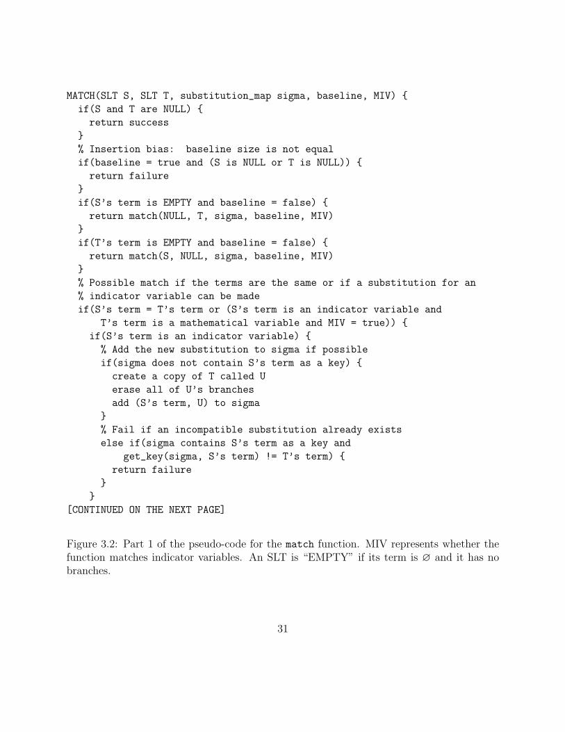
The match function takes two SLT structs, S and T , an integer for whether to match

indicator variables, and an integer for whether the current SLT nodes lie along the baseline

(so, when first called, baseline = 1), and returns a matcher substitution σ for the two SLTs

if successful. If both SLTs are ∅, the match completes successfully (the base case). If either

SLT is empty (S = (∅) or T = (∅)), the function replaces it with ∅. If only one of the

29

SLTs is ∅ and baseline = 1, the match fails because of the insertion bias (the baselines of

the two SLTs are different sizes). If the terms contained within the current nodes of S and

T are the same, recursively call the function on each of their corresponding branches (so,

using S’s Above node and T ’s Above node, etc.) and return success only if all those calls

are successful.

If match indicator variables = 1 and S’s term is an indicator variable v and T ’s

term is a mathematical variable t, check if vσ = v or vσ = t: if either are true, add v → t to

σ and recursively call the function on each branch as if the terms were the same; if neither

are true, the match fails because an indicator variable cannot be substituted for two different

terms simultaneously.

If the term in S’s current node is a substitution variable v, check if vσ = v or vσT

(where, if T = ∅, set T = (∅)). If neither are true, the match fails like before. If either

are true, create a temporary SLT U = T . Then consider each pair of the corresponding

branches of S and T : for each pair, if both branches exist (the nodes are not ∅), erase the

branch in U and recursively call the function on those branches. If the match fails for any

of these recursive calls, or the number of Argument branches for S and T are not equal,

return failure. Additionally, if S has a Next branch but T does not, the match fails because

S’s next node doesn’t have anything to match. Finally, if T has a Next branch and S does

not and baseline = 1, the match fails because a substitution variable cannot match multiple

nodes along the baseline. If it passes all these cases successfully, the match succeeds. If S’s

term was not a substitution variable, the match fails.

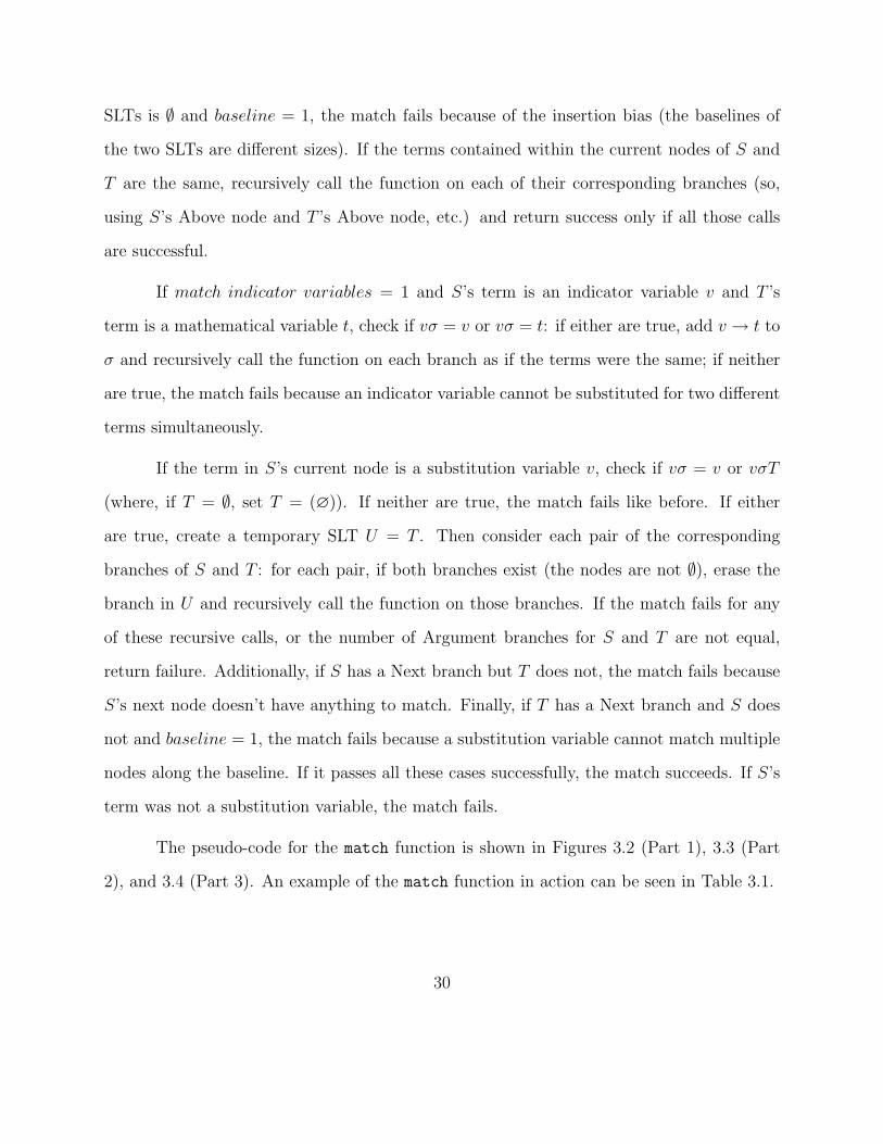
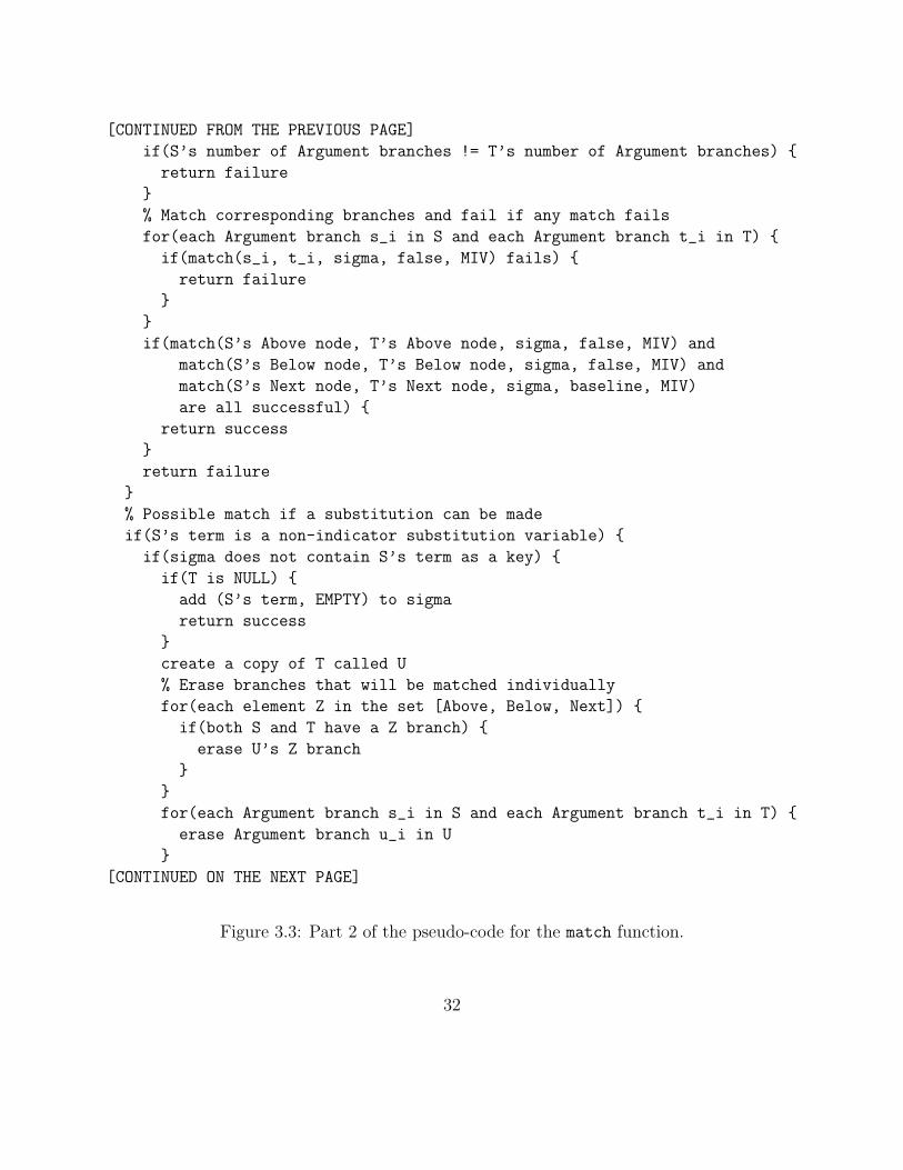
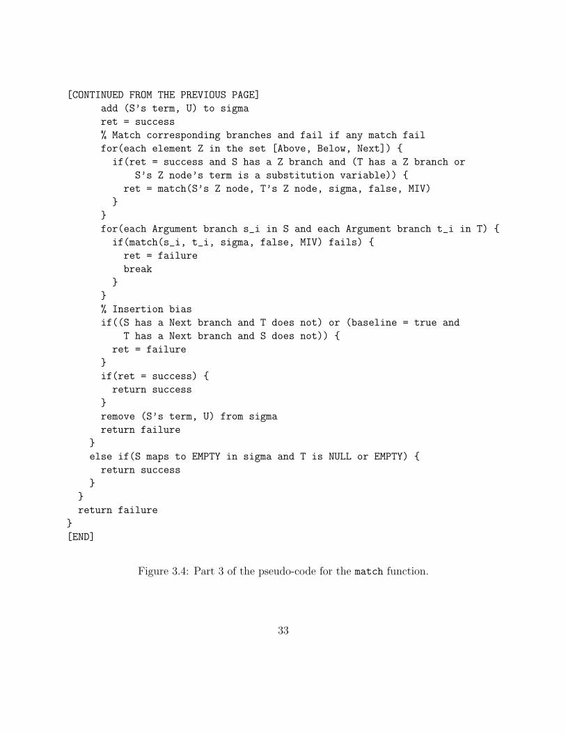
The pseudo-code for the match function is shown in Figures 3.2 (Part 1), 3.3 (Part

2), and 3.4 (Part 3). An example of the match function in action can be seen in Table 3.1.

30

MATCH(SLT S, SLT T, substitution_map sigma, baseline, MIV)

if(S and T are NULL)

return success

% Insertion bias: baseline size is not equal

if(baseline = true and (S is NULL or T is NULL))

return failure

if(S’s term is EMPTY and baseline = false)

return match(NULL, T, sigma, baseline, MIV)

if(T’s term is EMPTY and baseline = false)

return match(S, NULL, sigma, baseline, MIV)

% Possible match if the terms are the same or if a substitution for an

% indicator variable can be made

if(S’s term = T’s term or (S’s term is an indicator variable and

T’s term is a mathematical variable and MIV = true))

if(S’s term is an indicator variable)

% Add the new substitution to sigma if possible

if(sigma does not contain S’s term as a key)

create a copy of T called U

erase all of U’s branches

add (S’s term, U) to sigma

% Fail if an incompatible substitution already exists

else if(sigma contains S’s term as a key and

get_key(sigma, S’s term) != T’s term)

return failure

[CONTINUED ON THE NEXT PAGE]

Figure 3.2: Part 1 of the pseudo-code for the match function. MIV represents whether thefunction matches indicator variables. An SLT is “EMPTY” if its term is ∅ and it has nobranches.

31

[CONTINUED FROM THE PREVIOUS PAGE]

if(S’s number of Argument branches != T’s number of Argument branches)

return failure

% Match corresponding branches and fail if any match fails

for(each Argument branch s_i in S and each Argument branch t_i in T)

if(match(s_i, t_i, sigma, false, MIV) fails)

return failure

if(match(S’s Above node, T’s Above node, sigma, false, MIV) and

match(S’s Below node, T’s Below node, sigma, false, MIV) and

match(S’s Next node, T’s Next node, sigma, baseline, MIV)

are all successful)

return success

return failure

% Possible match if a substitution can be made

if(S’s term is a non-indicator substitution variable)

if(sigma does not contain S’s term as a key)

if(T is NULL)

add (S’s term, EMPTY) to sigma

return success

create a copy of T called U

% Erase branches that will be matched individually

for(each element Z in the set [Above, Below, Next])

if(both S and T have a Z branch)

erase U’s Z branch


erase Argument branch u_i in U

[CONTINUED ON THE NEXT PAGE]

Figure 3.3: Part 2 of the pseudo-code for the match function.

32

[CONTINUED FROM THE PREVIOUS PAGE]

add (S’s term, U) to sigma

ret = success

% Match corresponding branches and fail if any match fail

for(each element Z in the set [Above, Below, Next])

if(ret = success and S has a Z branch and (T has a Z branch or

S’s Z node’s term is a substitution variable))

ret = match(S’s Z node, T’s Z node, sigma, false, MIV)


if(match(s_i, t_i, sigma, false, MIV) fails)

ret = failure

break

% Insertion bias

if((S has a Next branch and T does not) or (baseline = true and

T has a Next branch and S does not))

ret = failure

if(ret = success)

return success

remove (S’s term, U) from sigma

return failure

else if(S maps to EMPTY in sigma and T is NULL or EMPTY)

return success

return failure

[END]

Figure 3.4: Part 3 of the pseudo-code for the match function.

33

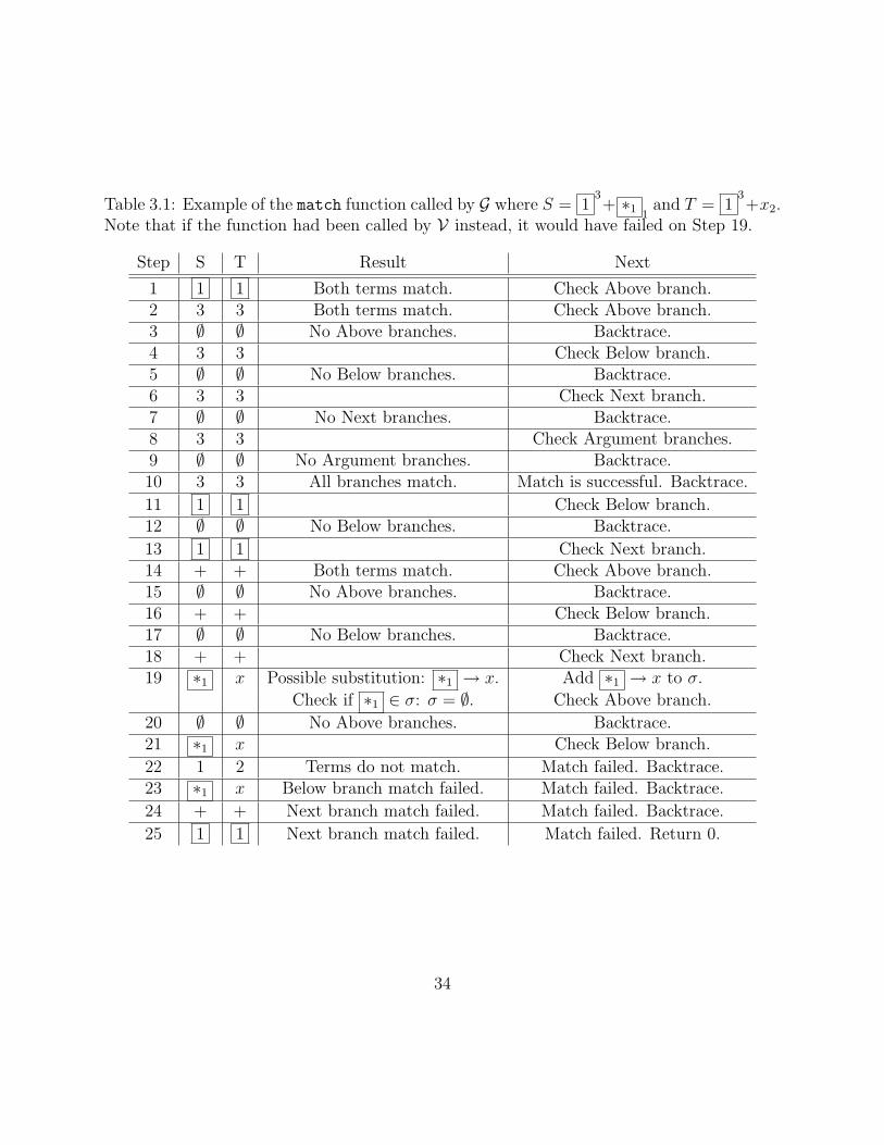
Table 3.1: Example of the match function called by G where S = 13+ ∗1 1

and T = 13+x2.

Note that if the function had been called by V instead, it would have failed on Step 19.

Step S T Result Next

1 1 1 Both terms match. Check Above branch.2 3 3 Both terms match. Check Above branch.3 ∅ ∅ No Above branches. Backtrace.4 3 3 Check Below branch.5 ∅ ∅ No Below branches. Backtrace.6 3 3 Check Next branch.7 ∅ ∅ No Next branches. Backtrace.8 3 3 Check Argument branches.9 ∅ ∅ No Argument branches. Backtrace.10 3 3 All branches match. Match is successful. Backtrace.

11 1 1 Check Below branch.12 ∅ ∅ No Below branches. Backtrace.

13 1 1 Check Next branch.14 + + Both terms match. Check Above branch.15 ∅ ∅ No Above branches. Backtrace.16 + + Check Below branch.17 ∅ ∅ No Below branches. Backtrace.18 + + Check Next branch.19 ∗1 x Possible substitution: ∗1 → x. Add ∗1 → x to σ.

Check if ∗1 ∈ σ: σ = ∅. Check Above branch.

20 ∅ ∅ No Above branches. Backtrace.21 ∗1 x Check Below branch.

22 1 2 Terms do not match. Match failed. Backtrace.23 ∗1 x Below branch match failed. Match failed. Backtrace.

24 + + Next branch match failed. Match failed. Backtrace.

25 1 1 Next branch match failed. Match failed. Return 0.

34

3.4.3 Finding the Most Common Specific Generalization for Substitutions

Finding the MSCG for two substitutions involves looking at both of the substitutions

and determining how they are similar to one another. The parts that are similar form the

generalization of the two substitutions while the parts that are different form two individual

instances of that generalization which, when composed with the generalization, produce the

original substitutions. The similar parts include not only identical parts but also terms that

share a common MSCG themselves. Thus the MSCG algorithm is made of two separate

functions: one that is called by the insertion function which finds the MSCG of two substi-

tutions (MSCGSub); and one that is called by the MSCGSub function which finds the MSCG of

two SLTs, if possible (MSCGSLT).

The MSCG algorithm takes two substitution maps τ and ρ and returns a substitution

map µ representing the generalization and two substitution maps σ1 and σ2 representing two

instances of µ that produce τ and ρ respectively. It iterates through each substitution

Si → Ti in τ = S1 → T1, . . . , Sn → Tn and compares it to ρ in order to determine if the

substitution is similar enough to generalize (and added to µ) or too different and must be

individualized (modifying σ1 and σ2 appropriately). It does this through calling MSCGSub.

Once all substitutions in τ have been considered, the function is finished; the substitutions

that remain in ρ which need to be added to σ2 are done so in the insert function as described

below. The algorithm is defined mathematically in Figure 3.5.

MSCGSub can handle the substitution Si → Ti in four different ways depending on the

content of ρ which Graf names BIND, FREEZE, MIX and DIVIDE. If ρ does not contain

the substitution variable Si then the substitution is unique to τ and is added to σ1 through

BIND (Definition 3.4). If ρ contains an identical substitution to Si → Ti then it is added to

µ with FREEZE (Definition 3.5). MIX (Definition 3.6) is used when ρ contains a conflicting

35

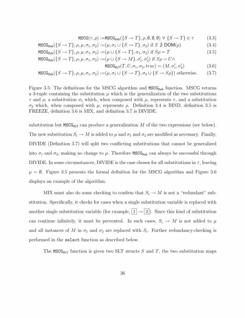
MSCG(τ, ρ) :=MSCGSub(S → T, ρ, ∅, ∅, ∅) ∀ S → T ∈ τ (3.3)

MSCGSub(S → T, ρ, µ, σ1, σ2) :=(µ, σ1 ∪ S → T, σ2) if S @ DOM(ρ) (3.4)

MSCGSub(S → T, ρ, µ, σ1, σ2) :=(µ ∪ S → T, σ1, σ2) if Sρ = T (3.5)

MSCGSub(S → T, ρ, µ, σ1, σ2) :=(µ ∪ S →M, σ′1, σ′2) if Sρ = U∧MSCGSLT(T, U, σ1, σ2, true) = (M,σ′1, σ

′2) (3.6)

MSCGSub(S → T, ρ, µ, σ1, σ2) :=(µ, σ1 ∪ S → T, σ2 ∪ S → Sρ) otherwise. (3.7)

Figure 3.5: The definitions for the MSCG algorithm and MSCGSub function. MSCG returnsa 3-tuple containing the substitution µ which is the generalization of the two substitutionsτ and ρ, a substitution σ1 which, when composed with µ, represents τ , and a substitutionσ2 which, when composed with µ, represents ρ. Definition 3.4 is BIND, definition 3.5 isFREEZE, definition 3.6 is MIX, and definition 3.7 is DIVIDE.

substitution but MSCGSLT can produce a generalization M of the two expressions (see below).

The new substitution Si →M is added to µ and σ1 and σ2 are modified as necessary. Finally,

DIVIDE (Definition 3.7) will split two conflicting substitutions that cannot be generalized

into σ1 and σ2, making no change to µ. Therefore MSCGSub can always be successful through

DIVIDE. In some circumstances, DIVIDE is the case chosen for all substitutions in τ , leaving

µ = ∅. Figure 3.5 presents the formal definition for the MSCG algorithm and Figure 3.6

displays an example of the algorithm.

MIX must also do some checking to confirm that Si →M is not a “redundant” sub-

stitution. Specifically, it checks for cases when a single substitution variable is replaced with

another single substitution variable (for example, 1 → 2 ). Since this kind of substitution

can continue infinitely, it must be prevented. In such cases, Si → M is not added to µ

and all instances of M in σ1 and σ2 are replaced with Si. Further redundancy-checking is

performed in the select function as described below.

The MSCGSLT function is given two SLT structs S and T , the two substitution maps

36

τ = 1 → 1, 2 → +, 3 → 52

+ 9, 4 → 4ρ = 2 → +, 3 → 3 ∗ 9, 4 → 10

µ = 2 → +, 3 → 56

7 9σ1 = 1 → 1, 4 → 4, 6 → 2, 7 → +σ2 = 4 → 10, 5 → 3, 6 → ∅, 7 → ∗

Figure 3.6: Example outcome of the MSCG algorithm. τ and ρ are sets of substitutions thatcould be seen in the middle of the insertion process. Note that they are not expressions bythemselves; as substitutions, they could be applied to many different expressions, such as

5 ∗ ( 3 2 1 ) 4 +1 or 12

2 3 + cos ( 4 + 9 ). MSCGSub uses BIND on 1 , FREEZE on

2 , MIX on 3 and DIVIDE on 4 . The call to MSCGSLT for 3 (comparing the conflicting

expressions in τ and ρ: 52

+ 9 and 3 ∗ 9) is enumerated as a step-by-step procedure inTable 3.2.

σ1 and σ2 used in MSCGSub, and whether S and T lie along the baseline (b). It returns the

generalized SLT M and the two substitution maps σ′1 and σ′2 which are modified to accom-

modate M . Starting at the root of the two SLTs, the function goes through comparing each

pair of corresponding nodes along all of their branches (Above, Below, Next and Argument)

through recursion to ensure that the entirety of both expressions are generalized. M is built

during the recursion, one node at a time, with each node corresponding to a node in S or T .

For each SLT node S = (s, A1, B1, X1, . . . , Xm, N1) and T = (t, A2, B2, Y1, . . . , Yn, N2),

the function compares s and t. If s = t then no more work is necessary; the corresponding

node in M is set to the term and the function continues by comparing S and T ’s branches.

If a common substitution for s and t already exists in σ1 and σ2 such that v → s ∈ σ1 and

v → t ∈ σ2 then the node in M is set to v and the function continues. If s is a substitution

variable then s → t is added to σ2, the node in M is set to s and the function continues.

Finally, if s and t cannot be generalized in any other way, a new substitution variable v is

37

created, v → s is added to σ1, v → t is added to σ2, the current node in M is set to v and

the function continues.

MSCGSLT fails if, at any point, S and T lie along the baseline and S = ∅ ⊕ T = ∅

(where ⊕ is XOR). This means that the baseline size of the two expressions is not equal

and, because of the baseline insertion bias, no generalization can be made. Assuming that it

doesn’t fail in any of its recursive calls, the function succeeds in producing a generalization

for the expressions S and T .

Technically, two different LATEX functions can be generalized as long as they have

the same number of arguments and the MSCG doesn’t fail otherwise. For example, cosx

(\cosx) and 1 (\hat1) can be generalized to 1 2 , but cosx and 12

(\frac12)

can’t because the former has one argument and the latter has two.

3.4.4 Selecting the Best Branch for Insertion

The select function chooses the child of the current substitution tree node that is

the most similar to an expression. It is given a substitution tree struct (τ,Σ) (the “current

node” in the index, where τ is a substitution contained in that node and Σ is its set of child

nodes), a substitution map ρ representing the SLT T to be inserted (ρ = 0 → T), and an

SLT struct P containing the path from the root of the index to the current node. It returns a

substitution tree struct from Σ that is the chosen branch if successful, or nothing otherwise.

The function first iterates through each element in Σ and sees if any of them match ρ; if so,

the element becomes the chosen branch and select succeeds. If none of τ ’s children are a

match, the function must look for any possible generalizations for ρ among its children. It

iterates through each element in Σ again, this time seeing if any of them are the MSCG for

ρ; if so, the function must check that the current node is not the index root and that the

38

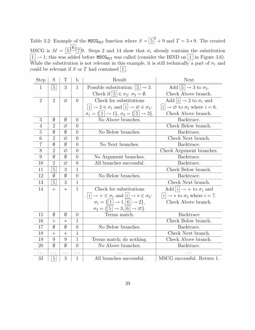
Table 3.2: Example of the MSCGSLT function where S = 52

+ 9 and T = 3 ∗ 9. The created

MSCG is M = 56

7 9. Steps 2 and 14 show that σ1 already contains the substitution

1 → 1; this was added before MSCGSLT was called (consider the BIND on 1 in Figure 3.6).While the substitution is not relevant in this example, it is still technically a part of σ1 andcould be relevant if S or T had contained 1 .

Step S T b Result Next

1 5 3 1 Possible substitution: 5 → 3. Add 5 → 3 to σ2.

Check if 5 ∈ σ2: σ2 = ∅. Check Above branch.

2 2 ∅ 0 Check for substitutions Add i → 2 to σ1 and

i → 2 ∈ σ1 and i → ∅ ∈ σ2: i → ∅ to σ2 where i = 6.

σ1 = 1 → 1, σ2 = 5 → 3. Check Above branch.3 ∅ ∅ 0 No Above branches. Backtrace.4 2 ∅ 0 Check Below branch.5 ∅ ∅ 0 No Below branches. Backtrace.6 2 ∅ 0 Check Next branch.7 ∅ ∅ 0 No Next branches. Backtrace.8 2 ∅ 0 Check Argument branches.9 ∅ ∅ 0 No Argument branches. Backtrace.10 2 ∅ 0 All branches successful. Backtrace.

11 5 3 1 Check Below branch.12 ∅ ∅ 0 No Below branches. Backtrace.

13 5 3 1 Check Next branch.

14 + ∗ 1 Check for substitutions Add i → + to σ1 and

i → + ∈ σ1 and i → ∗ ∈ σ2: i → ∗ to σ2 where i = 7.

σ1 = 1 → 1, 6 → 2, Check Above branch.

σ2 = 5 → 3, 6 → ∅.15 ∅ ∅ 0 Terms match. Backtrace16 + ∗ 1 Check Below branch.17 ∅ ∅ 0 No Below branches. Backtrace.18 + ∗ 1 Check Next branch.19 9 9 1 Terms match; do nothing. Check Above branch.20 ∅ ∅ 0 No Above branches. Backtrace.. . . . . . . . . . . . . . . . . .

33 5 3 1 All branches successful. MSCG successful. Return 1.

39

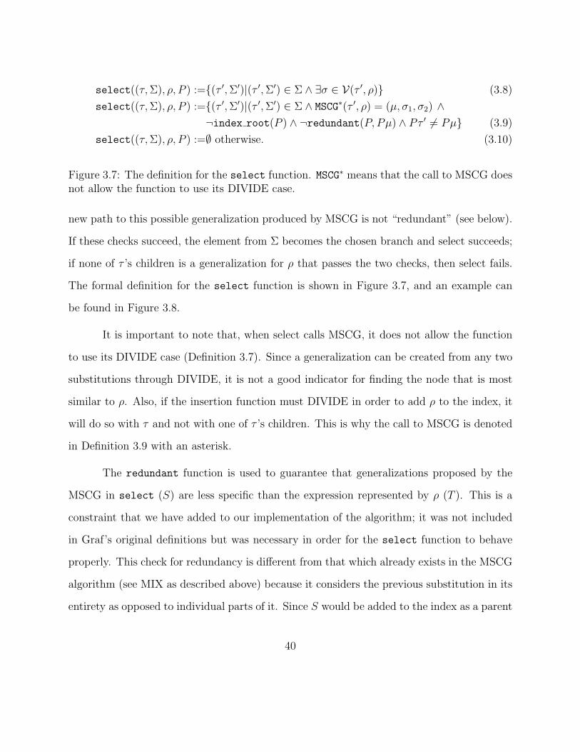
select((τ,Σ), ρ, P ) :=(τ ′,Σ′)|(τ ′,Σ′) ∈ Σ ∧ ∃σ ∈ V(τ ′, ρ) (3.8)

select((τ,Σ), ρ, P ) :=(τ ′,Σ′)|(τ ′,Σ′) ∈ Σ ∧ MSCG∗(τ ′, ρ) = (µ, σ1, σ2) ∧¬index root(P ) ∧ ¬redundant(P, Pµ) ∧ Pτ ′ 6= Pµ (3.9)

select((τ,Σ), ρ, P ) :=∅ otherwise. (3.10)

Figure 3.7: The definition for the select function. MSCG∗ means that the call to MSCG doesnot allow the function to use its DIVIDE case.

new path to this possible generalization produced by MSCG is not “redundant” (see below).

If these checks succeed, the element from Σ becomes the chosen branch and select succeeds;

if none of τ ’s children is a generalization for ρ that passes the two checks, then select fails.

The formal definition for the select function is shown in Figure 3.7, and an example can

be found in Figure 3.8.

It is important to note that, when select calls MSCG, it does not allow the function

to use its DIVIDE case (Definition 3.7). Since a generalization can be created from any two

substitutions through DIVIDE, it is not a good indicator for finding the node that is most

similar to ρ. Also, if the insertion function must DIVIDE in order to add ρ to the index, it

will do so with τ and not with one of τ ’s children. This is why the call to MSCG is denoted

in Definition 3.9 with an asterisk.

The redundant function is used to guarantee that generalizations proposed by the

MSCG in select (S) are less specific than the expression represented by ρ (T ). This is a

constraint that we have added to our implementation of the algorithm; it was not included

in Graf’s original definitions but was necessary in order for the select function to behave

properly. This check for redundancy is different from that which already exists in the MSCG

algorithm (see MIX as described above) because it considers the previous substitution in its

entirety as opposed to individual parts of it. Since S would be added to the index as a parent

40

∅

0 → ∗11

1 → 2 1 → 3

0 → 5

∅

0 → ∗11

1 → 2

1 → 3

1 → 4

0 → 5

Figure 3.8: Left: We want to insert x4 into a substitution tree which contains x2, x3 and

5. Starting at the root node (∅, 0 → ∗11 , 0 → 5), the select function can

choose between either of the root’s two children – in which case the insertion algorithm willrecur using the selected node as the new root – or fail, forcing the new expression to be

added as a new child of the root. It determines that 0 → ∗11 is the best child node for

recursion because ∗11 is a generalization of x4. For the next node ( 0 → ∗1

1 , 1 →2, 1 → 3), the select function fails because it can neither find a generalization of x4

in the two child nodes nor create a new one, and thus a generalization must be created using

0 → ∗11 through the MSCG algorithm. Right: The substitution tree after insertion.

for T , the function must ensure that T is an instance of S since following a branch in the

substitution tree is supposed to produce an expression that is more specific with each passing

node. Sometimes MSCG will offer an invalid generalization, forcing T to replace a term in S

with a substitution variable (for example, S = 1 +5, T = 1 + 2 ), and such generalizations

must be avoided. Thus the redundant function tells the select function which proposals

from the MSCG function to ignore. The only exception to this test is when the current node

the root substitution variable 0 in order to create the initial set of sub-trees from the root.

The formal definition for the redundant function is shown in Figure 3.9.

3.4.5 The Insertion Function

The insert function remains close to Graf’s original implementation as summarized

in Section 2.4. It is given a file containing a mathematical expression that has been converted

41

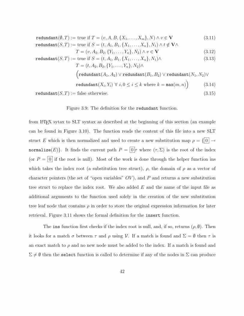
redundant(∅, T ) := true if T = (v, A,B, X1, . . . , Xm, N) ∧ v ∈ V (3.11)

redundant(S, T ) := true if S = (t, A1, B1, X1, . . . , Xn, N1) ∧ t /∈ V∧T = (v, A2, B2, Y1, . . . , Yn, N2) ∧ v ∈ V (3.12)

redundant(S, T ) := true if S = (t, A1, B1, X1, . . . , Xn, N1)∧ (3.13)

T = (t, A2, B2, Y1, . . . , Yn, N2)∧(redundant(A1, A2) ∨ redundant(B1, B2) ∨ redundant(N1, N2)∨

redundant(Xi, Yi) ∀ i, 0 ≤ i ≤ k where k = max(m,n))

(3.14)

redundant(S, T ) := false otherwise. (3.15)

Figure 3.9: The definition for the redundant function.

from LATEX sytax to SLT syntax as described at the beginning of this section (an example

can be found in Figure 3.10). The function reads the content of this file into a new SLT

struct E which is then normalized and used to create a new substitution map ρ = 0 →

normalize(E). It finds the current path P = 0 τ where (τ,Σ) is the root of the index

(or P = 0 if the root is null). Most of the work is done through the helper function ins

which takes the index root (a substitution tree struct), ρ, the domain of ρ as a vector of

character pointers (the set of “open variables” OV ), and P and returns a new substitution

tree struct to replace the index root. We also added E and the name of the input file as

additional arguments to the function used solely in the creation of the new substitution

tree leaf node that contains ρ in order to store the original expression information for later

retrieval. Figure 3.11 shows the formal definition for the insert function.

The ins function first checks if the index root is null, and, if so, returns (ρ, ∅). Then

it looks for a match σ between τ and ρ using V . If a match is found and Σ = ∅ then τ is

an exact match to ρ and no new node must be added to the index. If a match is found and

Σ 6= ∅ then the select function is called to determine if any of the nodes in Σ can produce

42

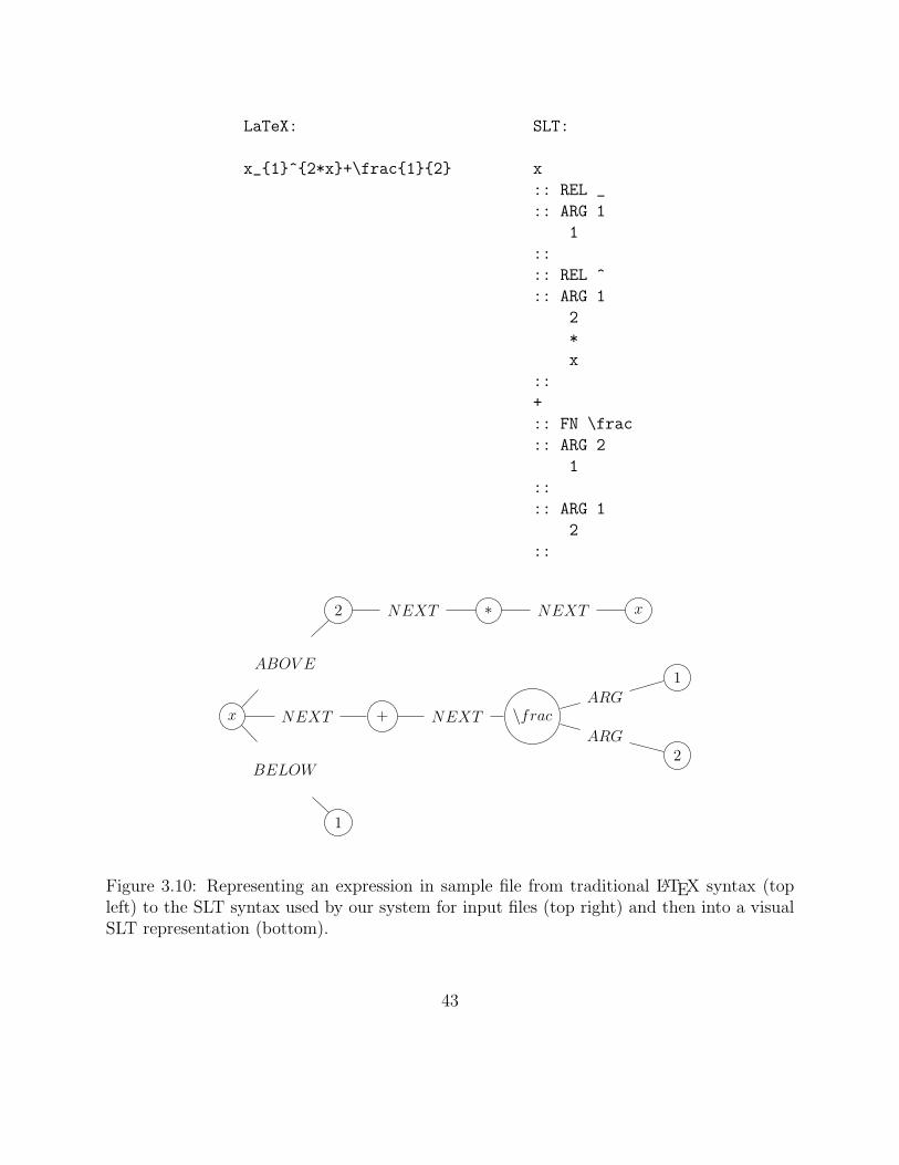
LaTeX: SLT:

x_1^2*x+\frac12 x

:: REL _

:: ARG 1

1

::

:: REL ^

:: ARG 1

2

*

x

::

+

:: FN \frac

:: ARG 2

1

::

:: ARG 1

2

::

x NEXT + NEXT \fracARG

1

ARG2

ABOV E

2 NEXT ∗ NEXT x

BELOW

1

Figure 3.10: Representing an expression in sample file from traditional LATEX syntax (topleft) to the SLT syntax used by our system for input files (top right) and then into a visualSLT representation (bottom).

43

a match or suitable generalization for ρ. It is given the composition of ρ and σ instead of

just ρ so it can be correctly compared to the elements in Σ. If select succeeds it returns

the child chosen for recursion, (τ ′,Σ′). The old path P is applied to τ ′ to generate the new

path, OV is updated with new substitution variables found in τ , and (τ ′,Σ′) is removed

from Σ. Then the result of the recursive call to ins is added to Σ (in effect replacing the

old child) and this updated substitution tree node is returned. If select fails then the only

node that matches ρ in (τ,Σ) is τ itself, so ρσ (without the substitution variables that are

already present in τ) is added to Σ as a new child for τ . If a match is not found, the function

must create a generalization for τ and ρ through the MSCG function. The generalization

µ replaces τ in the substitution tree node and two new children replace Σ: one containing

σ1 and having Σ as its set of children; the other containing σ2 combined with ρ (without

the substitution variables that were already present in τ) and having no children. This

replacement substitution tree node is returned and the function exits. Thus a generalization

can always be created if none of the nodes in the branch is a match to the newly inserted

expression.

3.5 The Retrieval Algorithm

Our innovations for Graf’s retrieval algorithm include using the search function not

only on the search query (which will only return exact matches), but also on each of the

query’s sub-expressions, and several variations of the query and its sub-expressions that are

generated by the retrieval algorithm. These variations are described later in this section;

however, it is important to note that all of these variations are expressions that contain

substitution variables themselves in order to match different expressions in the index. Since

now both sides of our matching comparison (the search query and the expressions in the

index) can potentially contain substitution variables, we must now introduce unification.

44

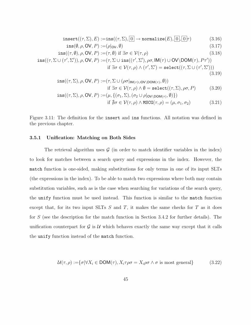
insert((τ,Σ), E) :=ins((τ,Σ), 0 → normalize(E), 0 , 0 τ) (3.16)

ins(∅, ρ,OV, P ) :=(ρ|OV, ∅) (3.17)

ins((τ, ∅), ρ,OV, P ) :=(τ, ∅) if ∃σ ∈ V(τ, ρ) (3.18)

ins((τ,Σ ∪ (τ ′,Σ′)), ρ,OV, P ) :=(τ,Σ ∪ ins((τ ′,Σ′), ρσ, IM(τ) ∪ OV\DOM(τ), P τ ′))

if ∃σ ∈ V(τ, ρ) ∧ (τ ′,Σ′) = select((τ,Σ ∪ (τ ′,Σ′)))(3.19)

ins((τ,Σ), ρ,OV, P ) :=(τ,Σ ∪ (ρσ|IM(τ)∪OV\DOM(τ), ∅))if ∃σ ∈ V(τ, ρ) ∧ ∅ = select((τ,Σ), ρσ, P ) (3.20)

ins((τ,Σ), ρ,OV, P ) :=(µ, (σ1,Σ), (σ2 ∪ ρ|OV\DOM(τ), ∅))if @σ ∈ V(τ, ρ) ∧ MSCG(τ, ρ) = (µ, σ1, σ2) (3.21)

Figure 3.11: The definition for the insert and ins functions. All notation was defined inthe previous chapter.

3.5.1 Unification: Matching on Both Sides

The retrieval algorithm uses G (in order to match identifier variables in the index)

to look for matches between a search query and expressions in the index. However, the

match function is one-sided, making substitutions for only terms in one of its input SLTs

(the expressions in the index). To be able to match two expressions where both may contain

substitution variables, such as is the case when searching for variations of the search query,

the unify function must be used instead. This function is similar to the match function

except that, for its two input SLTs S and T , it makes the same checks for T as it does

for S (see the description for the match function in Section 3.4.2 for further details). The

unification counterpart for G is U which behaves exactly the same way except that it calls

the unify function instead of the match function.

U(τ, ρ) :=σ|∀Xi ∈ DOM(τ), Xiτρσ = Xiρσ ∧ σ is most general (3.22)

45

Compared to G (definition 3.1), U (definition 3.22) contains σ on both sides of its

equality because σ is a unifier instead of simply a matcher.

3.5.2 Ranking Search Results

The search results are ranked by comparing each individual result to the original

search query, even if the result was found using a sub-expression or generalization. Compar-

isons for the ranking algorithm is based on a hybrid of the bipartite expression representation

[28] and the well-known bag-of-words model. Comparing expressions using the bipartite rep-

resentation makes a list of neighbor relationships for each of the two expressions. Each

element in these lists is a 5-tuple (s, n, r, p, b), where s is the symbol, n is a symbol neighbor-

ing s, r is the relationship between s and n (above, below, argument or next), p is the position

of s along the baseline, and b is a number representing the baseline that gets changed for

sub-expressions. For example, xx+1 = (x, x, above, 1, 1), (x,+, above, 1, 1), (x, 1, above, 1, 1),

(x,+, next, 1, 2), (x, 1, next, 1, 2), (+, 1, next, 2, 2). The bag-of-words approach also makes

a list for each expression, but the elements of this list are merely each of the symbols that

appear in the corresponding expression. For example, xx+1 = x, x,+, 1.

Both comparison functions calculate a rank between 0 and 1 by finding the set sim-

ilarity [11] on the number of matches and partial matches between the two lists. Partial

matches are found as a percentage matching of tuple elements. Elements themselves can

either match fully if they are equal or partially if their terms share a common type (vari-

able, constant, operator, function), so y is a closer match to x than 1. Partial matches are

chosen by a greedy matching algorithm. Using the set similarity forces both the number of

successful matches and the length of each expression to factor in to the rank. It also causes

identical matches to always be ranked at 100%.

46

The entire ranking algorithm is described in more detail in Section 3.5.6.

3.5.3 Creating Extended Variations of the Search Query

We make multiple variations of the search query by extending it in different ways.

An expression is extended by adding one or more unused substitution variables to each side

of the expression; the extension amount is set by the user and every possible variation is

created and used in the retrieval. For example, for the expression x+1 and extension amount

2, the variations include 1 x+ 1, x+ 1 1 , 1 2 x+ 1, 1 x+ 1 2 , and x+ 1 1 2 . This

is important in order to find similar expressions that are longer than the search query, such

as x + 1 + 2, because the baseline size bias implemented in the indexing algorithm would

otherwise cause these expressions to be ignored by the retrieval algorithm. For example, the

expression 1 x+1 matches 2x+1 which is similar (and thus relevant) to the original search

query x+ 1.

3.5.4 A Detailed Description of the Retrieval Algorithm

The retrieval algorithm is given the name of an SLT file, and the maximum amount

the query should be extended. The algorithm produces a vector of search results whose

elements are populated by the multiple separate searches that are performed for the query.

Each search result is its own C struct containing an SLT struct for the relevant expression,

a character pointer for the name of the document in which that expression is located, and a

double for the similarity of the result (as a percentage) used in ranking.

The algorithm then calls the search function on the query itself, storing the search

results that are returned in the search result vector. Next, it searches for all extended

variations of the search query. Then it searches for all sub-expressions of the search query,

including all of their nested sub-expressions: for example, the sub-expressions of the query

47

xx∗(y+1)+yn−1 are x∗(y+1), y+1, and n−1. Single term sub-expressions are ignored because

they skew the results due to their frequency (like searching for “the” in Google): for example,

we do not search for any sub-expressions of the query xx + y1. The algorithm also creates

generalized sub-expression term variations for each sub-expression. These variations replace

the node leading to a sub-expression with a substitution variable and strip away all other

terms: for example, the generalized sub-expression term variation for xx+1 + 1 is 1x+1

.

This variation allows the algorithm to find even more expressions containing similar sub-

expressions. Finally, the algorithm searches for all variations of all sub-expressions (including

nested sub-expressions) and produces the final search result vector that is sorted by rank

and then displayed to the user.

The search function takes the root of the index (τ,Σ) as a substitution tree struct,

the original search query Q and the current search query E as the substitution maps ξ =

0 → Q and ρ = 0 → E respectively, the current path P from the index root to τ as

an SLT struct, and the retrieval function X to be used in this particular search as a function

pointer. The retrieval functions include G, V and U (although V is not used). The current

search query for the first invocation of the search function is the same as the original search

query; however, both are needed to keep track of the search query given by the user when

subsequent searches (such as those on sub-expressions) are made.

The function first calls X on 0 → P and ρ. If X successfully returns a substitution

map (the matcher or unifier), then τ is a match to the query. If Σ = ∅ (the node is a leaf

and thus represents a specific mathematical expression) then τ ’s expression (or expressions if

identical expressions from multiple files were inserted into the index) is ranked and added to

the search result vector. If Σ 6= ∅ (the node has children and thus is a generalized expression

containing one or more substitution variables) then search recurs on each element in Σ. This

48

ensures that only exact matches are included in the results.

While this implementation of the retrieval algorithm worked fairly well, it overlooked

a few very relevant expressions during our preliminary test runs. Due to time constraints, we

were unfortunately forced to add a major behavioral change to the algorithm that, while im-

proving the quality of search results, decreases time and memory performance significantly.

This change was, in addition to searching the index for the query, sub-expressions of the

query, and extended variations of the query and its sub-expressions, to also search for varia-

tions of the query’s completely generalized baseline. A more elegant solution to our problem

of search result quality can be found in Section 3.5.5.

We create the completely generalized baseline by replacing each term on the baseline

of the original search query with a substitution variable. For example, x2 + 1 becomes

1 2 3 . We ignore the query’s Above, Below and Argument branches during this creation

because a substitution variable that lies along the baseline can match terms with or without

these branches ( 1 can match any expression with a baseline size of 1, including x, x2 or xxyz ).

We also create completely generalized baselines for the extended variations of the query (so,

continuing our example, we would also search for 1 2 3 4 and 1 2 3 4 5 , assuming

the default extension amount of 2).

Notice that the use of the completely generalized baseline causes many of the previous

searches to become unnecessary, because, for example, the results returned by a search for

x2 + 1 will always be a subset of the results returned by a search for 1 2 3 . In practice,

this means that all expressions in the index with the same baseline size as the query (as well

as slightly larger sizes, due to the extended queries) are added to the search result vector.

While our ranking algorithm ensures that irrelevant results do not appear among the top

search results, this unfortunate addition essentially produces a semi-exhaustive search of the

49

Table 3.3: Examples of the queries generated by the retrieval algorithm using the originalsearch query xx+1 + 5 and the default extension amount (2). The algorithm searches foreach of these variations and adds all matches to a vector of search results. The finishedvector is sorted by the ranking algorithm based on the matching expression’s similarity tothe original search query. Notice that the last three queries (starting with 1 2 3 ) arevariations of the completely generalized baseline; using these expressions as a search queriesmakes many of our other queries (including the original query) unnecessary because theymatch any expressions with a baseline size of 3, 4 or 5.

Search Queries Generated from xx+1 + 5

Original Query xx+1 + 5 Extended Sub-Exp. x+ 1 1 2

Extended Original 1 xx+1 + 5 Generalized Sub-Exp. Term 1x+1

Extended Original xx+1 + 5 1 Extended Gen. Sub-Exp. Term 1 2x+1

Extended Original 1 xx+1 + 5 2 Extended Gen. Sub-Exp. Term 1x+1

2

Extended Original 1 2 xx+1 + 5 Extended Gen. Sub-Exp. Term 1 2x+1

3

Extended Original xx+1 + 5 1 2 Extended Gen. Sub-Exp. Term 1 2 3x+1

Sub-Expression x+ 1 Extended Gen. Sub-Exp. Term 1x+1

2 3

Extended Sub-Exp. 1 x+ 1 Completely Gen. Baseline 1 2 3

Extended Sub-Exp. x+ 1 1 Completely Gen. Baseline 1 2 3 4

Extended Sub-Exp. 1 x+ 1 2 Completely Gen. Baseline 1 2 3 4 5

Extended Sub-Exp. 1 2 x+ 1

50

index and does not fully utilize the generality of Graf’s search function.

3.5.5 The Retrieval Algorithm: A More Elegant Solution

Upon post-experiment reflection, we have designed a more elegant solution to improve

the quality of our search results without resorting to the semi-exhaustive search enacted by

our use of the completely generalized baseline. Our solution is to create generalized variations

of the search query and its sub-expressions. These variations are similar to the generalized

sub-expressions but contain the whole expression (as opposed to just one term) and affect

all terms in the expression (as opposed to just terms containing sub-expressions) and are

thus more useful. The retrieval algorithm treats these new variations the same way that

it treats the extended variations of the query: by creating and searching for each variation

individually and adding the results produced by each search to the final search result vector.

This would replace our use of the completely generalized baseline, although that could be

re-introduced to the algorithm if such behavior was desired.

An expression is generalized by replacing one or more of its terms with substitution

variables. The retrieval algorithm would search on a complete set of all possible variations,

from replacing just a single term in the expression to replacing all but one of the terms

(replacing all of the terms would result in the completely generalized baseline, which is not

what we want). An example of a complete set of all possible generalized variations of a

search query can be seen in Table 3.4.

3.5.6 A Detailed Description of the Ranking Algorithm

Ranking is done through the rank function as shown in Definition 3.23. We use the

name “identity” to refer to the lists created by the functions in F (the bag-of-words and the

bipartite representation). An expression’s identity is stored in a C struct containing each

51

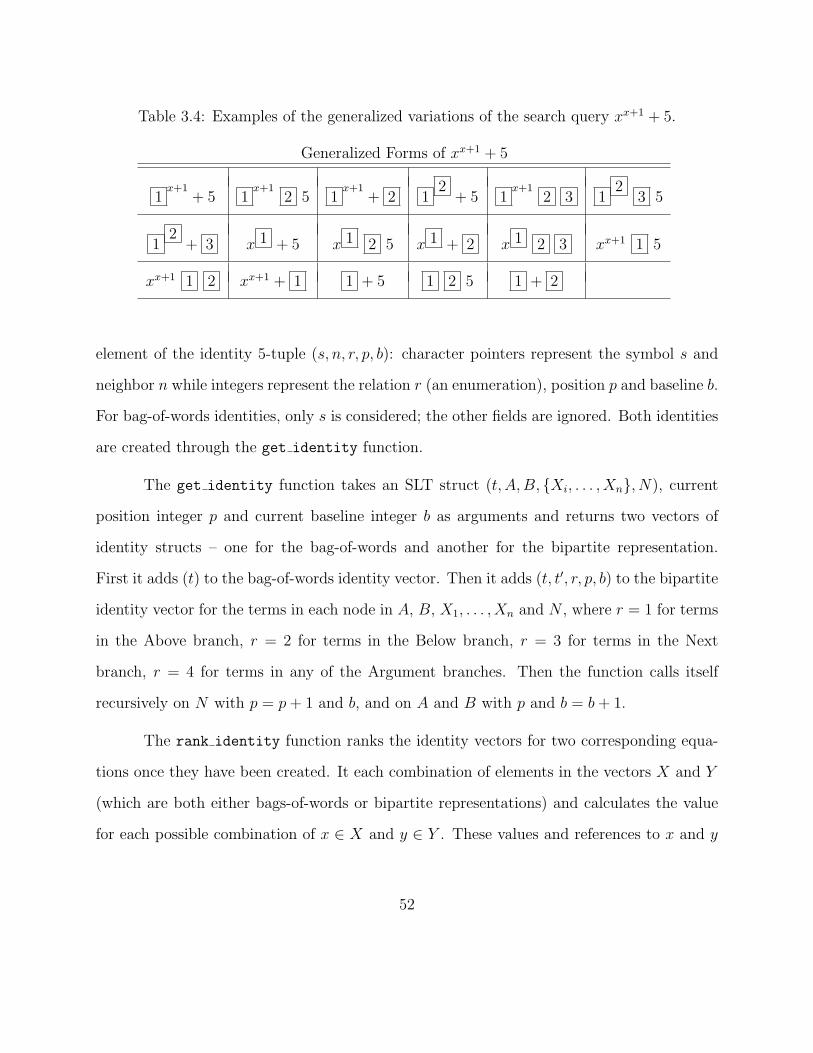
Table 3.4: Examples of the generalized variations of the search query xx+1 + 5.

Generalized Forms of xx+1 + 5

1x+1

+ 5 1x+1

2 5 1x+1

+ 2 12

+ 5 1x+1

2 3 12

3 5

12

+ 3 x 1 + 5 x 1 2 5 x 1 + 2 x 1 2 3 xx+1 1 5

xx+1 1 2 xx+1 + 1 1 + 5 1 2 5 1 + 2

element of the identity 5-tuple (s, n, r, p, b): character pointers represent the symbol s and

neighbor n while integers represent the relation r (an enumeration), position p and baseline b.

For bag-of-words identities, only s is considered; the other fields are ignored. Both identities

are created through the get identity function.

The get identity function takes an SLT struct (t, A,B, Xi, . . . , Xn, N), current

position integer p and current baseline integer b as arguments and returns two vectors of

identity structs – one for the bag-of-words and another for the bipartite representation.

First it adds (t) to the bag-of-words identity vector. Then it adds (t, t′, r, p, b) to the bipartite

identity vector for the terms in each node in A, B, X1, . . . , Xn and N , where r = 1 for terms

in the Above branch, r = 2 for terms in the Below branch, r = 3 for terms in the Next

branch, r = 4 for terms in any of the Argument branches. Then the function calls itself

recursively on N with p = p+ 1 and b, and on A and B with p and b = b+ 1.

The rank identity function ranks the identity vectors for two corresponding equa-

tions once they have been created. It each combination of elements in the vectors X and Y

(which are both either bags-of-words or bipartite representations) and calculates the value

for each possible combination of x ∈ X and y ∈ Y . These values and references to x and y

52

rank(e1, e2) =1

|F|∑f∈F

2(rank identity(f(e1), f(e2)))

|f(e1)|+ |f(e2)|(3.23)

Figure 3.12: The ranking algorithm for two expressions e1 and e2 which returns a valuebetween 0 and 1 ranking the expressions’ similarity to one another, similar to the Tanimotoset similarity metric. F = bag of words, bipartite representation contains the iden-tity functions which each take an expression and return the corresponding set of identitiesfor that expression. While these identity functions are combined in our code implementa-tion (see get identity), they are represented in this equation separately to show that it isflexible enough to allow more identity functions to be added in the future.

are stored in a C struct and added to a vector which, once all possible combinations have

been evaluated, is sorted based on value. The function then iterates through the this vector

and calculates the total ranking using the highest possible value whose corresponding values

x and y have not yet been used (a greedy match).

The value for two identities (si, ni, ri, pi, bi) and (sk, nk, rk, pk, bk) is calculated by

considering each pair in the tuple individually. For r, p, and b, the value is increased by 1 if

they are the same or 0 if they are different. For s and n, the value is increased by 1 if they are

the same symbol, 0.25 if they are the same symbol type – they’re both mathematical variables

(x and y), operators (+ and ∗), numbers (1 and 2), or functions (\cos and \frac) – or 0

if they are different symbols and different symbol types. We chose 0.25 as the intermittent

value because we tested 0.5 and felt that it caused the rank to be too high. This total value

is divided by 5 to compute a value between 0 and 1. For a bag-of-words identity, only s is

compared and the total value is not divided by 5.

53

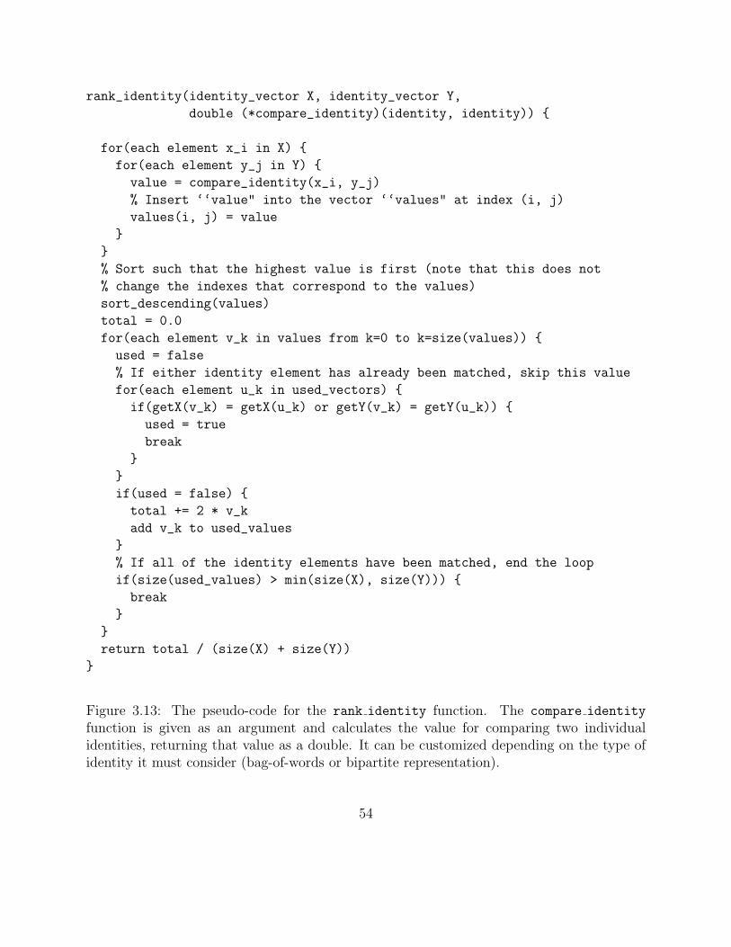
rank_identity(identity_vector X, identity_vector Y,

double (*compare_identity)(identity, identity))

for(each element x_i in X)

for(each element y_j in Y)

value = compare_identity(x_i, y_j)

% Insert ‘‘value" into the vector ‘‘values" at index (i, j)

values(i, j) = value

% Sort such that the highest value is first (note that this does not

% change the indexes that correspond to the values)

sort_descending(values)

total = 0.0

for(each element v_k in values from k=0 to k=size(values))

used = false

% If either identity element has already been matched, skip this value

for(each element u_k in used_vectors)

if(getX(v_k) = getX(u_k) or getY(v_k) = getY(u_k))

used = true

break

if(used = false)

total += 2 * v_k

add v_k to used_values

% If all of the identity elements have been matched, end the loop

if(size(used_values) > min(size(X), size(Y)))

break

return total / (size(X) + size(Y))

Figure 3.13: The pseudo-code for the rank identity function. The compare identity

function is given as an argument and calculates the value for comparing two individualidentities, returning that value as a double. It can be customized depending on the type ofidentity it must consider (bag-of-words or bipartite representation).

54

3.6 Summary

In summary, we have implemented Graf’s substitution tree insertion and search func-

tions for use in our own indexing and retrieval system for mathematical expressions. We

have made some small but necessary changes to the functions while retaining their overall

behavior in order to accommodate our transition from indexing predicates to expressions

encoded in a layout-based format to preserve the spatial differences of their symbols. We

have included a bias in the insertion function in order to populate the substitution tree with

expressions effectively. We have modified the retrieval algorithm to conduct searches on the

query, sub-expressions of the query and other variations of the query in order to return all

relevant search results contained in the index. Finally, we have added a ranking algorithm to

sort search results based on the similarity of their symbols and the layout of those symbols

to the search query.

In the next chapter we perform an experiment to compare our novel substitution tree

MIR system to the mathematical search engine developed by Zanibbi and Yuan [29]. We

also present a discussion of these results in which we make observations about our system.

55

Chapter 4

Results and Discussion

This chapter presents the details of our experiment comparing our substitution tree

MIR system to Zanibbi and Yuan’s keyword-based MIR system [29]. We then analyze and

discuss the results of our experiment.

4.1 Experiment and Results

We used the precision-at-k performance metric (which measures the relevance of the

top k results retrieved during a search [27]) to test the top k = 20 results of 10 test search

queries. Our search queries and document database were the same that Zanibbi and Yuan

used in their experiment [29]. We evaluated our results through an online survey that was

completed by 10 college upperclassmen in the Computer Science, Math and Engineering

fields (students with an advanced knowledge of mathematics). The survey contained 20

questions randomly ordered for each participant to prevent effects arising from presenting

retrieval results in a fixed order. Each of the 10 search queries appeared twice: once with

the top 20 results using Zanibbi and Yuan’s Lucene keyword-based system, and again with

the top 20 results using our substitution tree system. All expressions were shown as pictures

created using latex2html. Each question asked the participant to individually judge the 20

search results on their similarity to the query “in terms of both the similarity in symbols

between the query and candidate expressions and in their spatial arrangement.” Each search

result was rated as either “not similar at all,” “somewhat similar” or “very similar/identical.”

56

Table 4.1: Precision-at-k (k = 20) for 10 search queries (collection: 24,479 expressionsfrom 50 LATEX documents). Ten participants rated the results as “not similar at all” (0),“somewhat similar” (0.5) or “very similar/identical” (1.0). The mean ratings for the top 5results and top 20 results for Zanibbi and Yuan’s Lucene keyword-based system [29] and oursubstitution tree system are shown below as percentages.

Top 5 Results Top 20 ResultsQuery Expression Lucene Sub. Tree Lucene Sub. Tree

1 80.0 40.0 78.3 29.8

2 43.0 43.0 18.3 17.3

3 49.0 37.0 25.8 15.8

4 32.0 95.0 38.0 65.0

5 50.0 47.0 22.5 18.8

6 40.0 34.0 13.3 9.0

7 61.0 38.0 26.3 12.5

8 38.8 35.8 11.5 13.0

9 69.0 78.0 31.0 29.8

10 49.0 37.0 14.3 10.5

Mean (µ) 51.1 48.4 27.9 22.2Standard Deviation (σ) 14.9 20.8 19.6 16.7

57

This rating was converted to the numerical scale (0, 0.5, 1.0) and averaged for each result to

calculate the mean rating. The mean rating of the top 5 and top 20 results for each query

was averaged to produce the final results that appear in Table 4.1.

We indexed 24,479 expressions from 50 LATEX documents into a 12 GB file in about

6 minutes using a server with 2 Intel Xeon X5670 2.93 GHz processors with 24 cores and a

total of 95 GB of RAM. Our system contained fewer expressions than Zanibbi and Yuan’s

because it ignores expressions containing only one symbol (which appear far too frequently

to be useful) or over 100 symbols (which take up far too much space). Retrieval for nine of

the queries took between 2 seconds for query 1 to 2.5 minutes for query 10 (retrieval for query

3 took 12 minutes), largely dependent on the size of the search query and its sub-expressions

(all queries except for 3, 6 and 10, took 22 seconds or less), and returned between 4992 search

results for query 2 to 13266 search results for query 6. Queries with more sub-expressions

seemed to return more results due to the extra searches made using those sub-expressions.

As seen in the table, the substitution tree system performs comparably to the Lucene

system in many cases, but can also perform much better or much worse. However, the top

1 result was rated “identical” for all 10 search queries using the substitution tree system,

but for only 7 using the Lucene system (queries 1, 4, and 7 did not list the identical match

first, but did list it in their top 20). Table 4.2 compares the top 20 results from each system

for query 4; tables for the other queries are located in the Appendix (Chapter 6). The

Appendix also includes tables showing the specific LATEX syntax for each expression and the

distribution of ratings given by the participants of our experiment for the top 20 results of

each query.

58

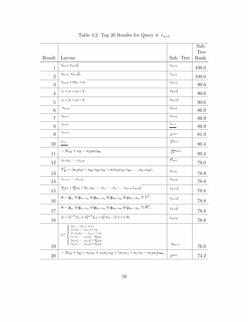
Table 4.2: Top 20 Results for Query 4: en+1

Sub.Tree

Result Lucene Sub. Tree Rank

1 100.0

2 100.0

3 90.6

4 90.6

5 90.6

6 86.9

7 86.9

8 86.9

9 81.9

10 80.4

11 80.4

12 79.0

13 78.8

14 78.8

15 78.8

16 78.8

17 78.8

18 78.8

19 76.0

20 74.2

59

4.2 Discussion

We can observe the main strength of our substitution tree system through query 4

where it vastly outperforms its Lucene counterpart both in the mean ratings obtained from

our experiment and the quality of its top 20 search results (as shown in Table 4.2). Our

system finds many relevant results through sub-expression matching which is apparent in the

consistency of results containing n+1 and n+2 (sometimes even as a superscript rather than

a subscript). It also ranks results identical to query 4 before non-identical results, unlike

the Lucene system which ranks six non-identical results higher than the identical results.

This may exemplify the detriment of the TF-IDF ranking method: since TF-IDF is heavily

influenced by documents in the index, it can rank relevant (and identical) results lower simply

because they occur more often. While this might be a good idea for text information retrieval,

it does not seem as effective for mathematical expressions, especially since a document

referencing the same expression multiple times often increases its importance.

The mean ratings for both the top 5 results and top 20 results of queries 2, 5, 6, and 8

are comparable between the two systems. The Lucene system produced much better results

for queries 3 and 10, suggesting that our system has difficulty with larger expressions. Both

systems would perform better if the database contained a larger set of more closely related

documents (as opposed to a set of 50 random documents in the broad field of physics). Plus,

since the queries were selected randomly from the database, some of them are probably not

good examples of likely queries that would be entered by real users.

One problem with our experiment is that our system doesn’t add single symbol ex-

pressions to its index while the Lucene system does. This is why the Lucene system does

so much better in our test on query 1: 17 of its top 20 results are the expression d which

most of our participants deemed “very similar/identical” to the query (d,). Since our sys-

60

tem did not index those expressions, the results were skewed in favor of the Lucene system.

However, our rationale for not indexing single symbol expressions – because they appear

too frequently to be useful search results – still seems legitimate; besides, searching for an

expression like d, is like searching Google for the word “the.” Furthermore, while indexing

single symbol expressions would not create many new nodes in our index (due to our use of

indicator variables), each of those nodes would contain references to a substantial number

of documents (since most LATEX documents contain single symbol expressions).

Results from our system found through sub-expression matching seem to be more

prominent for smaller queries (such as query 4). This is probably due to the behavior of our

ranking algorithm which determines the rank of a search result by comparing that result to

the original search query. For example, the expression n + 1 would be ranked much higher

when compared to the query en+1 than to the query en+1 + 1 simply because it has greater

symbol and size disparities with the latter, but it seems like n + 1 is just as relevant to

both queries. Thus, instead of ranking sub-expression matches by comparing them to the

original search query, our system should compare sub-expression matches to the original

sub-expression (and then have the rank weighted somehow so that sub-expressions are not

ranked at 100% when they are not identical to the original search query). Additionally, the

ranking algorithm should consider the frequency of a sub-expression in a search query so that

sub-expression matches are ranked higher if the sub-expression appears more than once in

the original search query (for example, compare the expression n+ 1 to the queries en+1 + 1

and en+1 + fn+1).

4.2.1 The Effects of LATEX Formatting

LATEX formatting has a great effect on our system as shown in the top 20 results of

queries 5, 7 and 9 and their comparatively low mean ratings. Query 5 begins with \mathcal,

61

query 7 begins with \mathbf, and query 9 begins with \,. Our system emphasizes these

terms (perhaps because they appear at the start of the queries) during retrieval. While our

system is successful in this aspect – all of the top 20 results for the three queries begin with

\mathcal, \mathbf, and \, respectfully – it affected the experiment because the participants

were looking for shared variables rather than shared formatting and therefore rated these

queries’ results lower. This could have been a flaw in our experiment since we only showed

our participants images of the expressions and told them to rate results based on their

similarity to the query in symbols and symbol layout, not formatting.

This all could have been avoided if our system simply ignored these formatting terms.

For example, the result ranked fourth by our system for query 9 (as seen in Table 6.12) looks

identical to query 9 yet is still ranked lower than non-identical results. However, we can see

why when we look at the original LATEX for the two expressions:

Query: \,\Omega_\tau a

Fourth Result: \,\Omega_\tau a\,

Since the \, adds two extra terms to the expression, our system ranks it as only 73.2%

similar to a query to which it should be identical. Thus it might be prudent for our system

to ignore such terms when indexing expressions because formatting has such a significant

effect on our system’s retrieval and ranking algorithms while having little to no effect on the

visual and mathematical similarity of two expressions. On the other hand, if a user enters a

formatting term in a search query, that user likely wants to see results which share the same

formatting; this seems rather unlikely, though.

62

4.2.2 The Shortcomings of the Insertion Bias

Our addition of a bias on the baseline size of an expression during its insertion into

the index also had a major and noticeable impact on our system’s search results. Most of

the top 20 results produced by our system are visually similar in size to the query, while the

results produced by the Lucene system vary dramatically. Since the searches for our system

used the default extension amount of 2, their results were restricted to a baseline size equal

to the query or up to two greater than the query unless they were matched on a search of

one of the query’s sub-expressions. This hurt our results because they seem to miss some

relevant results that the Lucene system finds – including results 5 and 10 for query 2, results

4-10 for query 3 and results 4 and 5 for query 10 (see Tables 6.5, 6.6 and 6.13) – simply

because they have larger baseline sizes.

The obvious solution would be to have our system conduct its searches using a larger

extension amount. However, what’s the right amount in order to retrieve all relevant results

from the index while maintaining low time costs? For our system to find the same result

for query 3 that the Lucene system found and ranked as its 9th result, we would need to

set the extension amount to 18; compared to the time costs we already experienced for our

searches at extension amount 2, the increase would be ridiculous. The main problem is

that our retrieval algorithm cannot fully compensate for the effects of the insertion bias on

indexing. While we chose this bias in part because the disparity in size between a search

query and search result has a significant impact on that result’s relevancy (results often

become less relevant as they become larger because of all the superfluous symbols), we see

from our experiment that this is not always the case, especially when the query itself (or an

expression very similar to the query) is contained within a larger expression (as seen in the

Lucene system’s results for query 3).

63

Note that this problem has to do with how expressions are retrieved from the index

(and how they are indexed in the first place), not how expressions are ranked. We have

full confidence in the effectiveness of our ranking algorithm (besides the modifications with

ranking sub-expression matches as noted above) – we just need to be able to find relevant

results from the index before we can rank them.

4.3 Summary

Our experiment demonstrates that our novel substitution tree MIR system is compa-

rable to Zanibbi and Yuan’s keyword-based vector-space Lucene MIR system. As exemplified

in our system’s perfect performance in the top 1 search results, our system’s ranking algo-

rithm, which is based only on structural similarity, seems to work better than the Lucene

system’s ranking algorithm, which is based in part on an expression’s frequency in the index.

Our system’s retrieval algorithm successfully finds results using the sub-expressions of search

queries, providing further strength to the quality of our search results. Unfortunately, our

system is negatively affected by two major factors: the presence of LATEX formatting in our

search queries and the expressions in our index, and the impact of the insertion bias on the

results that our retrieval algorithm is able to find. However, these are problems that could

be addressed and fixed in future implementations of our substitution tree MIR system.

Overall, while our experiment neither supports nor refutes our hypothesis that a

substitution tree indexing model would improve the relevance of search results over Zanibbi

and Yuan’s vector-space model, it does support our belief that further refinement of our

system is warranted.

64

Chapter 5

Conclusion and Future Work

Our hypothesis was that a substitution tree indexing model would improve the rele-

vance of search results over Zanibbi and Yuan’s vector-space model. While our experiment

neither supported nor refuted this hypothesis, we believe that further refinement of our novel

substitution tree MIR system using what we have learned through our experiment would

provide validation. Our implementation presents a promising first attempt at layout-based

substitution tree indexing and retrieval: it is comparable to another leading MIR system and

effective at finding relevant search results, especially results identical to the search query and

results relevant to the query’s sub-expressions.

Our contributions include: the design and implementation of substitution trees for

layout-based mathematical expressions (Chapter 2); the design and implementation of a sub-

stitution tree indexing algorithm for layout-based mathematical expressions, including the

introduction of an insertion bias (Chapter 3); the design and implementation of a substitu-

tion tree retrieval algorithm for layout-based mathematical expressions, including behavior

that retrieves expressions from the tree that are not identical yet still relevant (similar) to a

search query (Chapter 3); an experiment comparing our substitution tree MIR system to a

leading MIR system (Chapter 4); and a discussion analyzing the results of that experiment

and explaining specific ideas of how our system can be improved in future research based on

the findings from our experiment (Chapters 4 and 5).

Overall, we believe that we have provided a good foundation for future research in

65

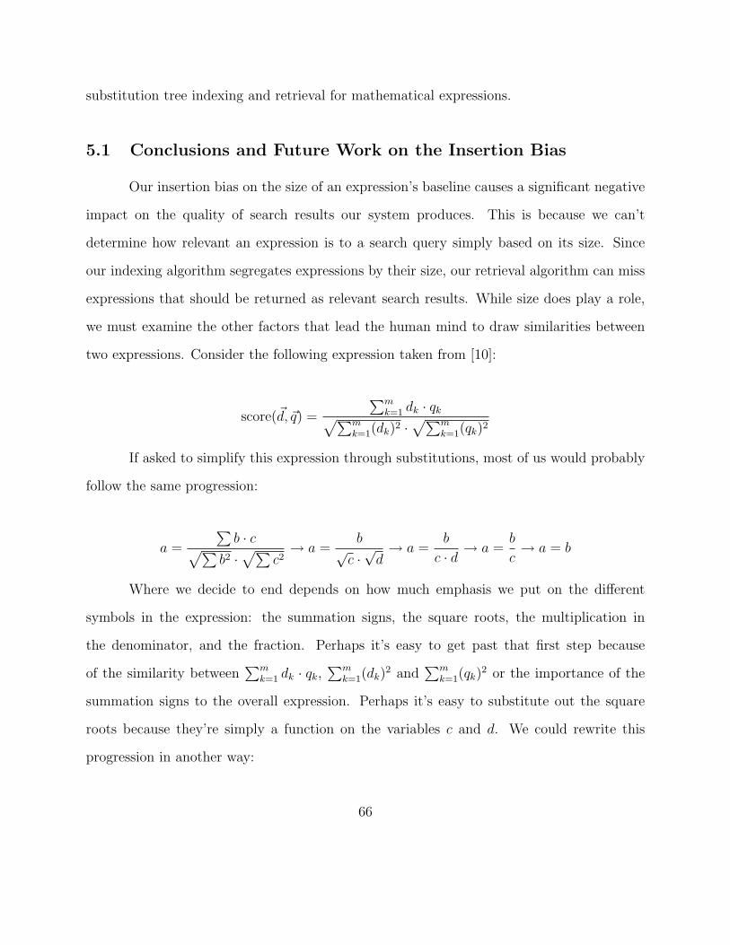
substitution tree indexing and retrieval for mathematical expressions.

5.1 Conclusions and Future Work on the Insertion Bias

Our insertion bias on the size of an expression’s baseline causes a significant negative

impact on the quality of search results our system produces. This is because we can’t

determine how relevant an expression is to a search query simply based on its size. Since

our indexing algorithm segregates expressions by their size, our retrieval algorithm can miss

expressions that should be returned as relevant search results. While size does play a role,

we must examine the other factors that lead the human mind to draw similarities between

two expressions. Consider the following expression taken from [10]:

score(~d, ~q) =

∑mk=1 dk · qk√∑m

k=1(dk)2 ·√∑m

k=1(qk)2

If asked to simplify this expression through substitutions, most of us would probably

follow the same progression:

a =

∑b · c√∑

b2 ·√∑

c2→ a =

b√c ·√d→ a =

b

c · d→ a =

b

c→ a = b

Where we decide to end depends on how much emphasis we put on the different

symbols in the expression: the summation signs, the square roots, the multiplication in

the denominator, and the fraction. Perhaps it’s easy to get past that first step because

of the similarity between∑m

k=1 dk · qk,∑m

k=1(dk)2 and

∑mk=1(qk)

2 or the importance of the

summation signs to the overall expression. Perhaps it’s easy to substitute out the square

roots because they’re simply a function on the variables c and d. We could rewrite this

progression in another way:

66

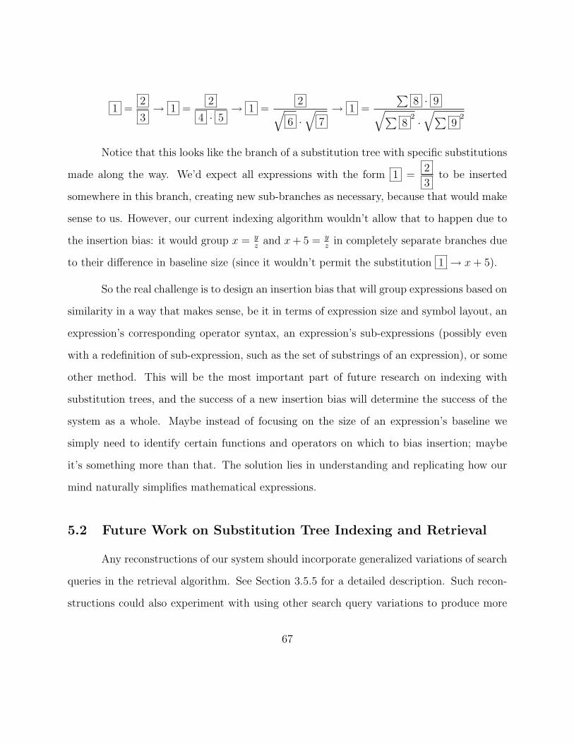
1 =2

3→ 1 =

2

4 · 5→ 1 =

2√6 ·√

7→ 1 =

∑8 · 9√∑

82 ·√∑

92

Notice that this looks like the branch of a substitution tree with specific substitutions

made along the way. We’d expect all expressions with the form 1 =2

3to be inserted

somewhere in this branch, creating new sub-branches as necessary, because that would make

sense to us. However, our current indexing algorithm wouldn’t allow that to happen due to

the insertion bias: it would group x = yz

and x+ 5 = yz

in completely separate branches due

to their difference in baseline size (since it wouldn’t permit the substitution 1 → x+ 5).

So the real challenge is to design an insertion bias that will group expressions based on

similarity in a way that makes sense, be it in terms of expression size and symbol layout, an

expression’s corresponding operator syntax, an expression’s sub-expressions (possibly even

with a redefinition of sub-expression, such as the set of substrings of an expression), or some

other method. This will be the most important part of future research on indexing with

substitution trees, and the success of a new insertion bias will determine the success of the

system as a whole. Maybe instead of focusing on the size of an expression’s baseline we

simply need to identify certain functions and operators on which to bias insertion; maybe

it’s something more than that. The solution lies in understanding and replicating how our

mind naturally simplifies mathematical expressions.

5.2 Future Work on Substitution Tree Indexing and Retrieval

Any reconstructions of our system should incorporate generalized variations of search

queries in the retrieval algorithm. See Section 3.5.5 for a detailed description. Such recon-

structions could also experiment with using other search query variations to produce more

67

relevant search results.

There are many other opportunities for future research concerning our system. First,

the index could be expanded from relying on an extensive document database to scraping

the World Wide Web to construct an even larger and more diverse index. The scraper

could start with the entire arXiv library of LATEX documents (from which our document

database was constructed). Regularly updating the index would ensure that it contains

expressions from the most current technical, mathematical and scientific papers. Second, a

user interface could be created that allows users to enter search queries more easily. Since

currently queries must be entered in LATEX syntax through a terminal prompt, our system is

not very user-friendly, especially to potential users who don’t have advanced mathematical

knowledge. This user interface could also include additional options on how the retrieval

and ranking algorithms should behave: for example, a user might want to emphasize search

results that match specific symbols and ignore results that do not contain those symbols.

Third, our system could be streamlined by an expert low-level programmer to be more time

and memory efficient.

Unlike the system created by Kohlhase and Sucan [14], we do not add sub-expressions

to our substitution tree index. This would dramatically increase the size of our index, and

the added benefit to the retrieval algorithm would largely overlap with its current behavior of

searching for the sub-expressions of a query along with the query itself. However, this might

be worth exploring for other cases which would otherwise be overlooked. For example, if we

search for the expression xx+1 in an index containing the expression x ∗ (x + 1), the latter

would not be returned as a relevant result unless the user set the extension amount to 4 (so

that the expression matches our extended sub-expression search query 1 2 3 x + 1 4 ).

If sub-expressions had been added to the index, then the expression x+ 1 would have been

68

inserted as a sub-expression of x ∗ (x+ 1) and would match any search for x+ 1. Thus this

could be a useful addition in the future.

Some of Kohlhase and Sucan’s other innovations could also be useful for incorporation

into our system. For example, their system is designed to accept generalized search queries

(already containing a substitution variable) for when a user only remember parts of an

expression. This feature could easily be implemented in our retrieval algorithm.

Another important problem with our system becomes apparent when considering

the apply function described in the previous section: making substitutions for SLTs with

Next branches (a baseline size larger than one) is done incorrectly in situations where the

substitution variable has an Above, Below or Argument branch. For example, applying the

substitution 1 → x + 1 to the expression x 12

will produce xx+12instead of x(x+1)2 . Note

that, with our baseline insertion bias, this situation will never happen with terms in the

baseline itself. The most efficient way of fixing this mistake would be to completely overhaul

the system by changing the fundamental structure of SLTs to allow them to contain another

SLT instead of a term, thereby making it easier to substitute nested expressions correctly in

such circumstances.

While we believe that our current ranking algorithm (based on a combination of

the bag-of-words and bipartite representation methods) is effective, there is always room for

improvement. Fortunately, the abstraction present in our rank identity function allows the

implementation of additional identity functions that would cause the rank to be weighted

based on other factors. For example, creating an identity function that prefers matching

neighboring symbols over matching symbols spread across an expression could improve the

quality of search results.

Finally, our normalization of mathematical variable names could be extended for other

69

symbol types such as constants or operators. Each of these symbols would be normalized

to their own corresponding type of indicator variable so an indicator variable that replaces

a mathematical variable cannot match an indicator variable that replaces another symbol

type. This would make it easier for the retrieval algorithm to match similar expressions,

and the ranking function would ensure that expressions with symbols that match the query

will still be ranked higher than those without matching symbols. For example, the query

x+ 1 seems more similar to x+ 2 than to x+x because, since the non-matching symbol is a

constant, expressions which replace that symbol with another constant seem more relevant.

The same is true for x + y and x − y because of the mathematical similarity of plus and

minus.

70

Chapter 6

Appendix

The tables provided in this chapter show the results of our experiment in greater detail

including both the side-by-side image comparison of and the ratings distributions given by

participants for the top 20 results for each of our search queries using the two MIR systems.

71

Table 6.1: The mean ratings (including standard deviation, abbreviated as SD) for the top5 and top 20 results for Zanibbi and Yuan’s Lucene keyword-based system [29] and oursubstitution tree system are shown below as percentages. The mean and standard deviationof each column is shown in the bottom two rows.

Top 5 Top 20Lucene Sub. Tree Lucene Sub. Tree

Query Mean SD Mean SD Mean SD Mean SD

1 80.0 0.0 40.0 33.5 78.3 11.3 29.8 16.72 43.0 37.4 43.0 39.0 18.3 24.7 17.3 23.83 49.0 36.7 37.0 43.4 25.8 27.2 15.8 23.84 32.0 32.5 95.0 5.0 38.0 38.0 65.0 25.65 50.0 34.8 47.0 30.3 22.5 25.8 18.8 23.46 40.0 35.5 34.0 41.7 13.3 23.9 9.0 24.37 61.0 21.6 38.0 48.0 26.3 29.4 12.5 27.58 38.8 50.0 35.8 37.8 11.5 28.2 13.0 22.29 69.0 34.9 78.0 21.7 31.0 32.3 29.8 37.0

10 49.0 38.3 37.0 47.1 14.3 27.4 10.5 26.9Mean (µ) 51.1 32.2 48.4 34.8 27.9 26.8 22.2 25.1

SD (σ) 14.9 13.2 20.8 13.2 19.6 6.8 16.7 5.1

72

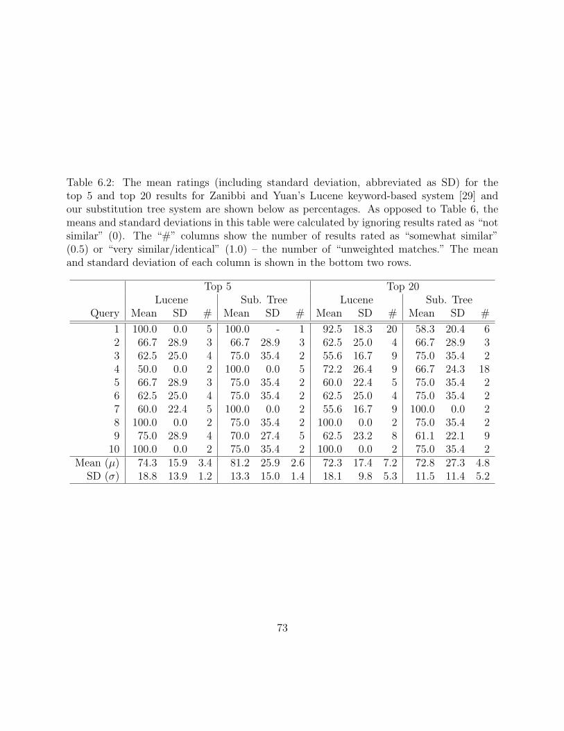
Table 6.2: The mean ratings (including standard deviation, abbreviated as SD) for thetop 5 and top 20 results for Zanibbi and Yuan’s Lucene keyword-based system [29] andour substitution tree system are shown below as percentages. As opposed to Table 6, themeans and standard deviations in this table were calculated by ignoring results rated as “notsimilar” (0). The “#” columns show the number of results rated as “somewhat similar”(0.5) or “very similar/identical” (1.0) – the number of “unweighted matches.” The meanand standard deviation of each column is shown in the bottom two rows.

Top 5 Top 20Lucene Sub. Tree Lucene Sub. Tree

Query Mean SD # Mean SD # Mean SD # Mean SD #

1 100.0 0.0 5 100.0 - 1 92.5 18.3 20 58.3 20.4 62 66.7 28.9 3 66.7 28.9 3 62.5 25.0 4 66.7 28.9 33 62.5 25.0 4 75.0 35.4 2 55.6 16.7 9 75.0 35.4 24 50.0 0.0 2 100.0 0.0 5 72.2 26.4 9 66.7 24.3 185 66.7 28.9 3 75.0 35.4 2 60.0 22.4 5 75.0 35.4 26 62.5 25.0 4 75.0 35.4 2 62.5 25.0 4 75.0 35.4 27 60.0 22.4 5 100.0 0.0 2 55.6 16.7 9 100.0 0.0 28 100.0 0.0 2 75.0 35.4 2 100.0 0.0 2 75.0 35.4 29 75.0 28.9 4 70.0 27.4 5 62.5 23.2 8 61.1 22.1 9

10 100.0 0.0 2 75.0 35.4 2 100.0 0.0 2 75.0 35.4 2Mean (µ) 74.3 15.9 3.4 81.2 25.9 2.6 72.3 17.4 7.2 72.8 27.3 4.8

SD (σ) 18.8 13.9 1.2 13.3 15.0 1.4 18.1 9.8 5.3 11.5 11.4 5.2

73

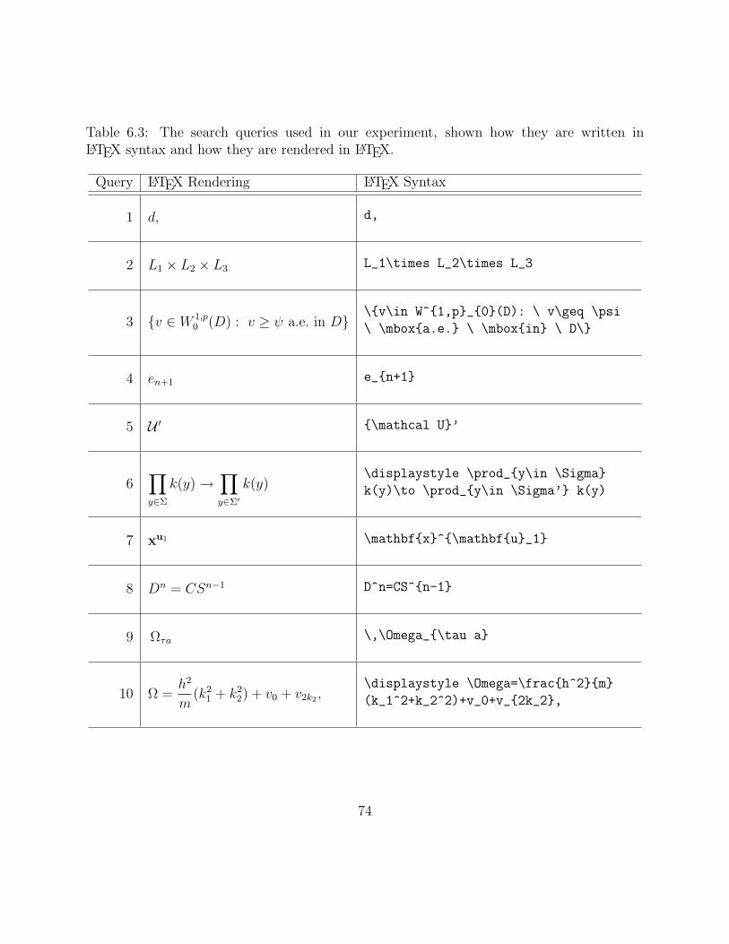
Table 6.3: The search queries used in our experiment, shown how they are written inLATEX syntax and how they are rendered in LATEX.

Query LATEX Rendering LATEX Syntax

1 d, d,

2 L1 × L2 × L3 L_1\times L_2\times L_3

3 v ∈ W 1,p0 (D) : v ≥ ψ a.e. in D

\v\in W^1,p_0(D): \ v\geq \psi

\ \mboxa.e. \ \mboxin \ D\

4 en+1 e_n+1

5 U ′ \mathcal U’

6∏y∈Σ

k(y)→∏y∈Σ′

k(y)\displaystyle \prod_y\in \Sigma

k(y)\to \prod_y\in \Sigma’ k(y)

7 xu1 \mathbfx^\mathbfu_1

8 Dn = CSn−1 D^n=CS^n-1

9 Ωτa \,\Omega_\tau a

10 Ω =h2

m(k2

1 + k22) + v0 + v2k2 ,

\displaystyle \Omega=\frach^2m

(k_1^2+k_2^2)+v_0+v_2k_2,

74

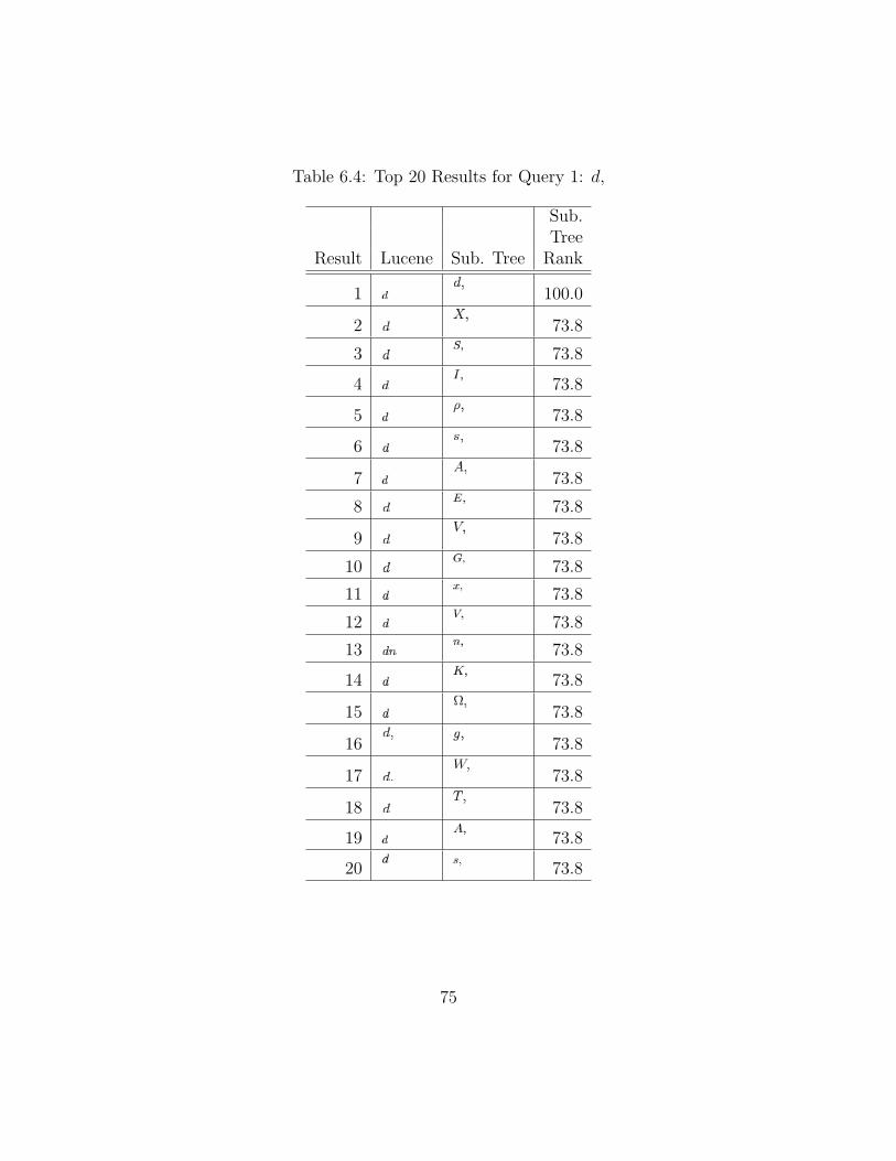
Table 6.4: Top 20 Results for Query 1: d,

Sub.Tree


1 100.0

2 73.8

3 73.8

4 73.8

5 73.8

6 73.8

7 73.8

8 73.8

9 73.8

10 73.8

11 73.8

12 73.8

13 73.8

14 73.8

15 73.8

16 73.8

17 73.8

18 73.8

19 73.8

20 73.8

75

Table 6.5: Top 20 Results for Query 2: L1 × L2 × L3

Sub.Tree


1 100.0

2 77.3

3 60.2

4 58.6

5 58.6

6 58.6

7 58.6

8 58.6

9 58.6

10 58.6

11 58.6

12 58.6

13 58.6

14 58.6

15 58.6

16 56.9

17 56.8

18 56.7

19 56.4

20 55.8

76

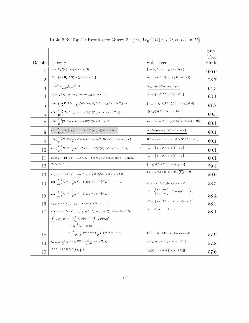
Table 6.6: Top 20 Results for Query 3: v ∈ W 1,p0 (D) : v ≥ ψ a.e. in D

Sub.Tree


1 100.0

2 78.7

3 64.3

4 63.1

5 61.7

6 60.3

7 60.1

8 60.1

9 60.1

10 60.1

11 60.1

12 59.4

13 59.0

14 58.5

15 58.4

16 58.2

17 58.1

18 57.9

19 57.8

20 57.6

77

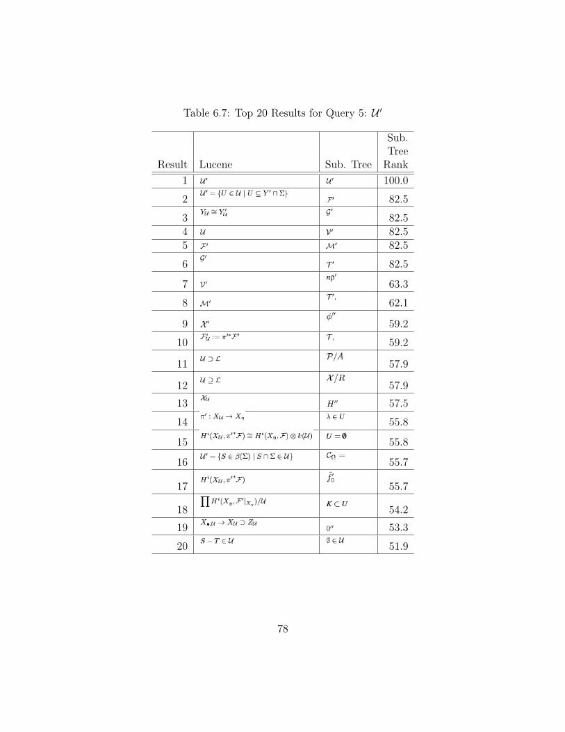
Table 6.7: Top 20 Results for Query 5: U ′

Sub.Tree


1 100.0

2 82.5

3 82.54 82.55 82.5

6 82.5

7 63.3

8 62.1

9 59.2

10 59.2

11 57.9

12 57.9

13 57.5

14 55.8

15 55.8

16 55.7

17 55.7

18 54.2

19 53.3

20 51.9

78

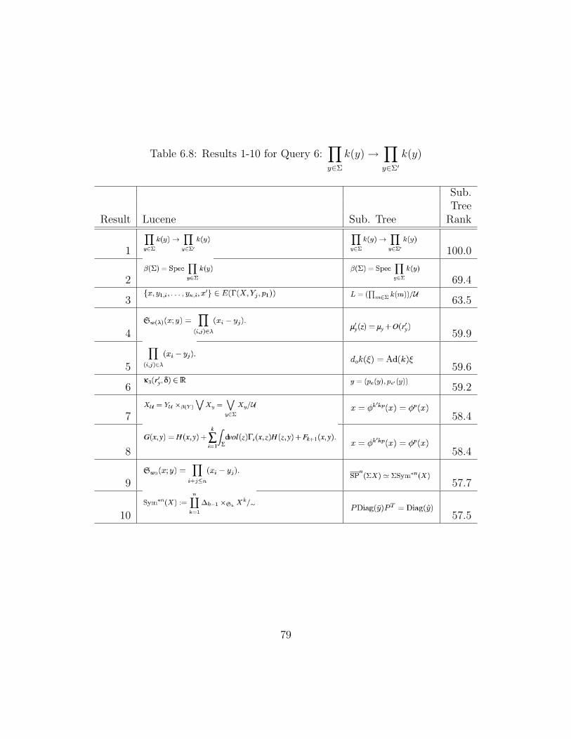
Table 6.8: Results 1-10 for Query 6:∏y∈Σ

k(y)→∏y∈Σ′

k(y)

Sub.Tree


1 100.0

2 69.4

3 63.5

4 59.9

5 59.6

6 59.2

7 58.4

8 58.4

9 57.7

10 57.5

79

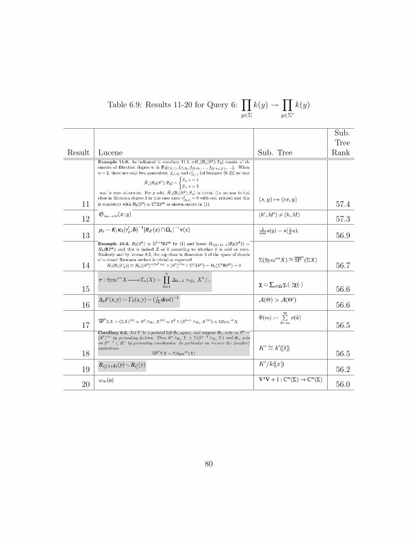
Table 6.9: Results 11-20 for Query 6:∏y∈Σ

k(y)→∏y∈Σ′

k(y)

Sub.Tree


11 57.4

12 57.3

13 56.9

14 56.7

15 56.6

16 56.6

17 56.5

18 56.5

19 56.2

20 56.0

80

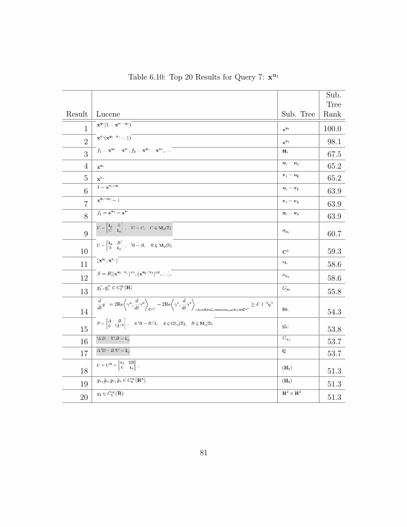
Table 6.10: Top 20 Results for Query 7: xu1

Sub.Tree


1 100.0

2 98.1

3 67.5

4 65.2

5 65.2

6 63.9

7 63.9

8 63.9

9 60.7

10 59.3

11 58.6

12 58.6

13 55.8

14 54.3

15 53.8

16 53.7

17 53.7

18 51.3

19 51.3

20 51.3

81

Table 6.11: Top 20 Results for Query 8: Dn = CSn−1

Sub.Tree


1 100.0

2 73.83 70.8

4 70.2

5 68.2

6 67.4

7 66.5

8 66.4

9 66.3

10 66.1

11 65.6

12 65.4

13 64.9

14 64.9

15 64.9

16 64.6

17 64.2

18 64.1

19 63.9

20 63.9

82

Table 6.12: Top 20 Results for Query 9: Ωτa

Sub.Tree


1 100.0

2 84.4

3 84.4

4 73.2

5 70.8

6 70.1

7 68.6

8 68.6

9 67.5

10 61.9

11 61.8

12 60.9

13 60.3

14 60.3

15 60.3

16 60.3

17 60.3

18 60.3

19 60.1

20 60.1

83

Table 6.13: Results 1-10 for Query 10: Ω =h2

m(k2

1 + k22) + v0 + v2k2 ,

Sub.Tree


1 100.0

2 87.3

3 69.2

4 64.1

5 63.1

6 63.0

7 62.9

8 62.5

9 61.5

10 61.0

84

Table 6.14: Results 11-20 for Query 10: Ω =h2

m(k2

1 + k22) + v0 + v2k2 ,

Sub.Tree


11 61.0

12 60.9

13 60.8

14 59.9

15 59.7

16 59.2

17 58.9

18 58.9

19 58.9

20 58.9

85

Table 6.15: The statistical mode (the most frequent) distribution of the ratings given byparticipants in our experiment for the top 5 and top 20 search results of Zanibbi and Yuan’sLucene system and our substitution tree system. Entries represent: (number of “not similar”ratings, number of “somewhat similar” ratings, number of “very similar/identical” ratings).

Lucene Substitution TreeQuery Top 5 Top 20 Top 5 Top 20

1 (0,0,5) (0,3,17) (4,0,1) (14,5,1)2 (2,2,1) (16,3,1) (2,2,1) (17,2,1)3 (1,3,1) (11,8,1) (3,1,1) (18,1,1)4 (3,2,0) (11,5,4) (0,0,5) (2,12,6)5 (2,2,1) (15,4,1) (3,1,1) (18,1,1)6 (1,3,1) (16,3,1) (3,1,1) (18,1,1)7 (0,4,1) (11,8,1) (3,0,2) (18,0,2)8 (3,0,2) (18,0,2) (3,1,1) (18,1,1)9 (1,2,2) (12,6,2) (0,3,2) (11,7,2)

10 (3,0,2) (18,0,2) (3,1,1) (18,1,1)

86

Tab

le6.

16:

The

dis

trib

uti

onof

rati

ngs

give

nby

par

tici

pan

tsin

our

exp

erim

ent

for

the

top

20se

arch

resu

lts

ofquer

ies

1-5.

Eac

hen

try

conta

ins

the

rati

ngs

give

nby

Zan

ibbi

and

Yuan

’sL

uce

ne

syst

eman

dou

rsu

bst

ituti

ontr

eesy

stem

,in

that

order

,se

par

ated

by

aco

mm

a.E

ntr

ies

repre

sent:

(num

ber

of“n

otsi

milar

”ra

tings

,num

ber

of“s

omew

hat

sim

ilar

”ra

tings

,num

ber

of“v

ery

sim

ilar

/iden

tica

l”ra

tings

).

Res

ult

Quer

y1

Quer

y2

Quer

y3

Quer

y4

Quer

y5

1(0

,4,6

),(0

,0,1

0)(0

,0,1

0),(

0,0,

10)

(0,0

,10)

,(0,

0,10

)(0

,7,3

),(0

,0,1

0)(0

,0,1

0),(

0,0,

10)

2(0

,4,6

),(5

,5,0

)(0

,8,2

),(0

,7,3

)(0

,6,4

),(0

,7,3

)(0

,7,3

),(0

,0,1

0)(1

,5,4

),(5

,4,1

)3

(0,4

,6),

(5,5

,0)

(7,3

,0),

(4,6

,0)

(9,1

,0),

(9,1

,0)

(5,4

,1),

(0,1

,9)

(7,3

,0),

(5,4

,1)

4(0

,4,6

),(5

,5,0

)(8

,2,0

),(8

,2,0

)(3

,7,0

),(8

,2,0

)(1

0,0,

0),(

0,2,

8)(1

,8,1

),(2

,7,1

)5

(0,4

,6),

(5,5

,0)

(4,6

,0),

(8,2

,0)

(3,7

,0),

(9,1

,0)

(10,

0,0)

,(0,

2,8)

(6,4

,0),

(5,4

,1)

6(0

,4,6

),(4

,6,0

)(6

,4,0

),(8

,2,0

)(3

,7,0

),(9

,1,0

)(0

,1,9

),(0

,6,4

)(6

,4,0

),(5

,4,1

)7

(0,4

,6),

(5,5

,0)

(6,4

,0),

(7,3

,0)

(4,5

,1),

(9,1

,0)

(0,0

,10)

,(0,

6,4)

(2,8

,0),

(7,3

,0)

8(0

,4,6

),(5

,5,0

)(6

,4,0

),(8

,2,0

)(1

,8,1

),(8

,2,0

)(0

,0,1

0),(

2,7,

1)(6

,4,0

),(5

,4,1

)9

(0,4

,6),

(5,5

,0)

(6,4

,0),

(7,3

,0)

(2,7

,1),

(8,2

,0)

(0,1

,9),

(7,3

,0)

(6,4

,0),

(7,3

,0)

10(0

,4,6

),(5

,5,0

)(2

,8,0

),(8

,2,0

)(2

,7,1

),(8

,2,0

)(3

,5,2

),(1

,8,1

)(8

,2,0

),(9

,1,0

)11

(0,4

,6),

(4,6

,0)

(9,1

,0),

(8,2

,0)

(9,1

,0),

(8,2

,0)

(10,

0,0)

,(1,

8,1)

(7,3

,0),

(10,

0,0)

12(0

,4,6

),(5

,5,0

)(9

,1,0

),(8

,2,0

)(6

,4,0

),(9

,1,0

)(3

,4,3

),(4

,5,1

)(7

,3,0

),(1

0,0,

0)13

(0,3

,7),

(4,6

,0)

(9,1

,0),

(8,2

,0)

(10,

0,0)

,(9,

1,0)

(10,

0,0)

,(0,

7,3)

(9,1

,0),

(7,3

,0)

14(0

,4,6

),(5

,5,0

)(1

0,0,

0),(

9,1,

0)(7

,3,0

),(7

,3,0

)(3

,4,3

),(0

,6,4

)(1

0,0,

0),(

9,1,

0)15

(0,4

,6),

(5,5

,0)

(10,

0,0)

,(8,

2,0)

(7,3

,0),

(8,2

,0)

(6,2

,2),

(1,6

,3)

(10,

0,0)

,(9,

1,0)

16(0

,5,5

),(4

,6,0

)(1

0,0,

0),(

8,2,

0)(1

0,0,

0),(

8,2,

0)(1

0,0,

0),(

1,6,

3)(3

,5,2

),(1

0,0,

0)17

(0,5

,5),

(5,5

,0)

(10,

0,0)

,(10

,0,0

)(1

0,0,

0),(

9,1,

0)(1

0,0,

0),(

1,6,

3)(1

0,0,

0),(

10,0

,0)

18(0

,4,6

),(5

,5,0

)(8

,2,0

),(9

,1,0

)(9

,1,0

),(9

,1,0

)(9

,1,0

),(1

,5,4

)(9

,1,0

),(8

,2,0

)19

(0,4

,6),

(6,4

,0)

(10,

0,0)

,(10

,0,0

)(1

0,0,

0),(

8,2,

0)(5

,4,1

),(0

,1,9

)(1

0,0,

0),(

9,1,

0)20

(0,4

,6),

(4,6

,0)

(9,1

,0),

(8,2

,0)

(10,

0,0)

,(7,

3,0)

(9,0

,0),

(7,3

,0)

(9,1

,0),

(9,1

,0)

87

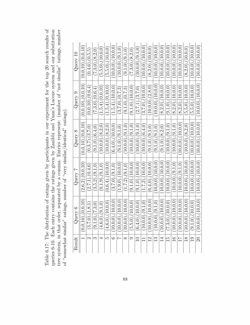
Tab

le6.

17:

The

dis

trib

uti

onof

rati

ngs

give

nby

par

tici

pan

tsin

our

exp

erim

ent

for

the

top

20se

arch

resu

lts

ofquer

ies

6-10

.E

ach

entr

yco

nta

ins

the

rati

ngs

give

nby

Zan

ibbi

and

Yuan

’sL

uce

ne

syst

eman

dou

rsu

bst

ituti

ontr

eesy

stem

,in

that

order

,se

par

ated

by

aco

mm

a.E

ntr

ies

repre

sent:

(num

ber

of“n

otsi

milar

”ra

tings

,num

ber

of“s

omew

hat

sim

ilar

”ra

tings

,num

ber

of“v

ery

sim

ilar

/iden

tica

l”ra

tings

).

Res

ult

Quer

y6

Quer

y7

Quer

y8

Quer

y9

Quer

y10

1(0

,0,1

0),(

0,0,

10)

(2,6

,2),

(0,0

,10)

(0,0

,10)

,(0,

0,10

)(0

,0,1

0),(

0,0,

10)

(0,0

,10)

,(0,

0,10

)2

(3,7

,0),

(1,8

,1)

(2,7

,1),

(0,4

,6)

(0,3

,7),

(3,7

,0)

(0,0

,10)

,(0,

6,4)

(0,4

,6),

(0,5

,5)

3(9

,1,0

),(7

,3,0

)(3

,5,2

),(9

,1,0

)(9

,1,0

),(6

,4,0

)(7

,3,0

),(0

,6,4

)(7

,3,0

),(8

,2,0

)4

(4,6

,0),

(9,1

,0)

(0,1

,9),

(9,1

,0)

(10,

0,0)

,(8,

2,0)

(1,5

,4),

(0,0

,10)

(5,5

,0),

(10,

0,0)

5(4

,6,0

),(1

0,0,

0)(0

,6,4

),(1

0,0,

0)(1

0,0,

0),(

8,2,

0)(1

,5,4

),(0

,10,

0)(5

,5,0

),(1

0,0,

0)6

(10,

0,0)

,(10

,0,0

)(3

,7,0

),(9

,1,0

)(6

,4,0

),(1

0,0,

0)(1

,5,4

),(1

0,0,

0)(1

0,0,

0),(

10,0

,0)

7(1

0,0,

0),(

10,0

,0)

(1,9

,0),

(10,

0,0)

(9,1

,0),

(9,1

,0)

(3,7

,0),

(0,7

,3)

(10,

0,0)

,(9,

1,0)

8(1

0,0,

0),(

10,0

,0)

(1,7

,2),

(9,1

,0)

(10,

0,0)

,(9,

1,0)

(9,1

,0),

(0,7

,3)

(9,1

,0),

(9,1

,0)

9(5

,5,0

),(1

0,0,

0)(9

,1,0

),(1

0,0,

0)(1

0,0,

0),(

9,1,

0)(9

,1,0

),(1

0,0,

0)(7

,3,0

),(8

,2,0

)10

(6,4

,0),

(10,

0,0)

(9,1

,0),

(10,

0,0)

(10,

0,0)

,(9,

1,0)

(2,7

,1),

(3,7

,0)

(10,

0,0)

,(9,

1,0)

11(1

0,0,

0),(

9,1,

0)(1

,7,2

),(1

0,0,

0)(1

0,0,

0),(

6,4,

0)(3

,7,0

),(1

0,0,

0)(1

0,0,

0),(

10,0

,0)

12(1

0,0,

0),(

10,0

,0)

(6,4

,0),

(10,

0,0)

(9,1

,0),

(9,1

,0)

(10,

0,0)

,(2,

8,0)

(8,2

,0),

(10,

0,0)

13(1

0,0,

0),(

9,1,

0)(1

0,0,

0),(

10,0

,0)

(9,1

,0),

(9,1

,0)

(10,

0,0)

,(10

,0,0

)(1

0,0,

0),(

10,0

,0)

14(1

0,0,

0),(

10,0

,0)

(10,

0,0)

,(10

,0,0

)(9

,1,0

),(8

,2,0

)(8

,2,0

),(1

0,0,

0)(1

0,0,

0),(

10,0

,0)

15(7

,3,0

),(1

0,0,

0)(1

0,0,

0),(

10,0

,0)

(10,

0,0)

,(9,

1,0)

(9,1

,0),

(10,

0,0)

(10,

0,0)

,(10

,0,0

)16

(10,

0,0)

,(10

,0,0

)(1

0,0,

0),(

9,1,

0)(1

0,0,

0),(

9,1,

0)(8

,2,0

),(1

0,0,

0)(1

0,0,

0),(

10,0

,0)

17(1

0,0,

0),(

10,0

,0)

(10,

0,0)

,(9,

1,0)

(10,

0,0)

,(10

,0,0

)(8

,2,0

),(1

0,0,

0)(1

0,0,

0),(

10,0

,0)

18(1

0,0,

0),(

10,0

,0)

(10,

0,0)

,(10

,0,0

)(1

0,0,

0),(

8,2,

0)(5

,5,0

),(1

0,0,

0)(8

,2,0

),(1

0,0,

0)19

(9,1

,0),

(10,

0,0)

(10,

0,0)

,(10

,0,0

)(1

0,0,

0),(

10,0

,0)

(5,5

,0),

(10,

0,0)

(10,

0,0)

,(10

,0,0

)20

(10,

0,0)

,(10

,0,0

)(1

0,0,

0),(

10,0

,0)

(10,

0,0)

,(10

,0,0

)(1

0,0,

0),(

10,0

,0)

(10,

0,0)

,(10

,0,0

)

88

Bibliography

[1] Moody Altamimi and Abdou Youssef. An extensive math query language. In ISCA

International Conference on Software Engineering and Data Engineering (SEDE-2007),

pages 57–63, Las Vegas, NV, 2007.

[2] Andrea Asperti, Ferruccio Guidi, Claudio Coen, Enrico Tassi, and Stefano Zacchiroli.

A content based mathematical search engine: Whelp. In Proc. Types for Proofs and

Programs 2004, volume 3839 of Lecture Notes in Computer Science, pages 17–32, 2006.

[3] D. Bolstein, J. Cordy, and R. Zanibbi. Applying compiler techniques to diagram

recognition. In Proc. International Conf. Pattern Recognition, volume 3, pages 123–

126, 2002.

[4] Pia Borlund. User-centered evaluation of information retrieval systems. In Information

Retrieval: Searching in the 21st Century, pages 21–37. Wiley, West Sussex, UK, 2009.

[5] J.R. Cordy. The TXL source transformation language. Science of Computer Program-

ming, 61(3):190–210, 2006.

[6] David Doermann. The indexing and retrieval of document images: A survey. Journal

on Computer Vision and Image Understanding, 70:287–298, June 1998.

[7] Peter Graf. Substitution tree indexing. In RTA ’95: Proceedings of the 6th Interna-

tional Conference on Rewriting Techniques and Applications, pages 117–131, London,

UK, 1995. Springer-Verlag.

89

[8] Peter Graf. Term Indexing. Lecture Notes in Artificial Intelligence 1053. Springer-

Verlag, Berlin, Germany, 1995.

[9] H. Hashimoto, Y. Hijikata, and S. Nishida. Incorporating breadth first search for in-

dexing MathML objects. In IEEE International Conf. Systems, Man and Cybernetics,

pages 3519–3523, Oct. 2008.

[10] Djoerd Hiemstra. Information retrieval models. In Information Retrieval: Searching

in the 21st Century, pages 1–19. Wiley, West Sussex, UK, 2009.

[11] Shahab Kamali and Frank Tompa. Improving mathematics retrieval. In Proc. DML

2009: Towards a Digital Mathematics Library, pages 37–48, Grand Bend, Canada, July

2009.

[12] Donald Knuth. The TEXbook. Addison Wesley, Reading, Massachusetts, 1986.

[13] Andrea Kohlhase and Michael Kohlhase. Reexamining the MKM value proposition:

From math web search to math web research. In Proc. Symposium Towards Mechanized

Mathematical Assistants, pages 313–326, Berlin, Heidelberg, 2007. Springer-Verlag.

[14] Michael Kohlhase and Ioan Sucan. A search engine for mathematical formulae. In

Jacques Calmet Testuo Ida and Dongming Wang, editors, Proc. Artificial Intelligence

and Symbolic Computation, number 4120 in LNAI, pages 241–253. Springer Verlag,

2006.

[15] Hsi-Jian Lee and Jiumn-Shine Wang. Design of a mathematical expression understand-

ing system. Pattern Recognition Letters, 18:289–298, 1997.

90

[16] Paul Libbrecht and Erica Melis. Methods for access and retrieval of mathematical

content in activemath. In Proc. International Congress on Mathematical Software,

volume 4151 of LNCS, pages 331–342. Springer-Verlag, 2006.

[17] William A. Martin. Computer input/output of mathematical expressions. In Proceed-

ings of the Second Symposium on Symbolic and Algebraic Manipulation, pages 78–89,

March 1971.

[18] Bruce R. Miller and Abdou Youssef. Technical aspects of the digital library of mathe-

matical functions. In Annals of Mathematics and Artificial Intelligence, pages 121–136.

May 2003.

[19] Robert Miner and Rajesh Munavalli. An Approach to Mathematical Search Through

Query Formulation and Data Normalization, volume 4573 of Lecture Notes in Artificial

Intelligence. 2007.

[20] Rajesh Munavalli and Robert Miner. MathFind: A math-aware search engine. In

SIGIR ’06: Proceedings of the 29th Annual International ACM SIGIR Conference on

Research and Development in Information Retrieval, page 735, New York, NY, 2006.

[21] Brigitte Pientka. Higher-order substitution tree indexing. In Catuscia Palamidessi,

editor, Logic Programming, volume 2916 of Lecture Notes in Computer Science, pages

377–391. Springer Berlin / Heidelberg, 2003.

[22] Gerald Salton and Michael J. McGill. Introduction to Modern Information Retrieval.

McGraw-Hill, Inc., New York, NY, USA, 1983.

[23] Clare M. So and Stephen M. Watt. Determining empirical characteristics of mathe-

matical expression use. In Proc. Mathematical Knowledge Management, volume 3863

91

of LNCS, pages 361–375. Springer, 2005.

[24] Ellen M. Voorhee. Overview of TREC 2003. In Proc. TREC, 2003.

[25] Abdou Youssef. Roles of math search in mathematics. In Jonathan Borwein and

William Farmer, editors, Mathematical Knowledge Management, volume 4108 of Lecture

Notes in Computer Science, pages 2–16. Springer Berlin / Heidelberg, 2006.

[26] Abdou Youssef. Methods of relevance ranking and hit-content generation in math

search. In Proc. Towards Mechanized Mathematical Assistants, pages 393–406, Berlin,

2007. Springer-Verlag.

[27] Richard Zanibbi and Dorothea Blostein. Recognition and retrieval of mathematics.

Int’l. Journal of Document Analysis and Recognition, 2011 to appear.

[28] Richard Zanibbi, Amit Pillay, Harold Mouchere, Christian Viard-Gaudin, and Dorothea

Blostein. Stroke-based performance metrics for handwritten mathematical expressions.

In Int’l Conf. Document Analysis and Recognition, pages 334–338, Beijing, 2011 to

appear.

[29] Richard Zanibbi and Bo Yuan. Keyword and image-based retrieval for mathematical

expressions. In Proc. Document Recognition and Retrieval XVIII, volume 7874 of Proc.

SPIE, pages OI1–OI9, San Francisco, CA, Jan. 2011.

[30] Jin Zhao, Min-Yen Kan, and Yin Leng Theng. Math information retrieval: User

requirements and prototype implementation. In Proc. ACM/IEEE Joint Conf. Digital

libraries, pages 187–196, New York, NY, USA, 2008.

92

layout-based substitution tree indexing and retrieval...

Documents