leading-edge boundary layer flow prandtl’s … · numerical solution of the appropriate...

LEADING-EDGE BOUNDARY LAYER FLOWPrandtl’s vision, current developments and future perspectives

V. Theofilis*, A.V. Fedorov** and S.S. Collis***

* E.T.S.I. Aeronáuticos, U. Politécnica de Madrid, E-28040 Madrid, SPAIN([email protected])** Moscow Institute of Physics and Technology, 141700 Moscow Region, RUSSIA([email protected])*** Sandia National Laboratories†, P.O. Box 5800, Albuquerque, NM 87185-0370, U.S.A([email protected])Abstract: The first viscous compressible three-dimensional BiGlobal linear instability

analysis of leading-edge boundary layer flow has been performed. Resultshave been obtained by independent application of asymptotic analysis andnumerical solution of the appropriate partial-differential eigenvalue problem.It has been shown that the classification of three-dimensional linearinstabilities of the related incompressible flow [13] into symmetric and anti-symmetric mode expansions in the chordwise coordinate persists forcompressible, subsonic flow-régime at sufficiently large Reynolds numbers.

Key words: Compressible Hiemenz flow, BiGlobal linear instability analysis

1. INTRODUCTION

In the context of external aerodynamics, the flow near the windwardstagnation line of a swept cylinder serves as a canonical model of a leading-edge boundary layer. Research into boundary-layer flows over an unsweptcylinder immediately followed the discovery of the boundary-layer conceptitself. Indeed, it was Prandtl’s interest in measuring the pressure on thesurface of a cylinder that led to the discovery, by Hiemenz [4], of an exactsolution of the incompressible Navier-Stokes equations that describes the

† Sandia is a multiprogram laboratory operated by Sandia Corporation, a Lockheed MartinCompany, for the United States Department of Energy's National Nuclear SecurityAdministration under contract DE-AC04-94AL85000.

2 Theofilis, Fedorov & Collis

stagnation point flow and bears his name. As the performance benefits ofswept wings were realized and demonstrated in Göttingen [5-6] this solutionwas extended to the well-known three-dimensional stagnation-line flow [10].

Concurrently with the extension of the swept Hiemenz solution to thecompressible régime by Reshotko and Beckwith [9], investigations into theinstability of leading-edge boundary layer commenced. The first instabilityresults were presented 50 years ago with the contributions of Görtler [1] andHämmerlin [2] to the meeting “Fifty Years Boundary-Layer Research,”celebrating Prandtl’s boundary-layer idea. Both those contributions dealtwith incompressible stagnation point (unswept Hiemenz) flow and putforward what has become known as the Görtler-Hämmerlin (GH) Ansatz,whereby linear disturbances of the leading-edge boundary layer inherit thefunctional dependence of the basic flow itself. Accordingly, the streamwiseand wall-normal disturbance velocity components are functions of the wall-normal coordinate and, in addition, the streamwise velocity componentdepends linearly on the chordwise spatial coordinate. This Ansatz was laterextended [3] and verified [11] for the incompressible stagnation line (sweptHiemenz) flow. These studies demonstrated that the most unstableeigenmode of the leading-edge boundary layer, denoted as the GH-mode,compares well with experiment and direct numerical simulation under linearconditions.

Recent advances in computing hardware and algorithms have permittedgeneralizations of the GH Ansatz in the context of BiGlobal linear theorybased on solution of partial-differential eigenvalue problems (EVP). Lin andMalik [7] discovered new eigenmodes besides the GH-mode, and Theofilis,Fedorov, Obrist and Dallmann [13] demonstrated that the instability ofincompressible three-dimensional swept leading-edge boundary-layer flow isamenable to analysis. The latter authors identified all (BiGlobal)eigenmodes as having a polynomial structure along the chordwise directionand reduced the partial-differential EVP to a system of one-dimensionalordinary-differential EVPs of the Orr-Sommerfeld class. The solution of thissystem delivers the complete three-dimensional instability characteristics forincompressible swept leading-edge boundary-layer flow.

The present contribution demonstrates that this reduction is also possiblefor compressible flows, albeit restricted to certain ranges of Reynolds andMach numbers. We proceed along lines analogous to [13] and arrive at theinstability characteristics of viscous compressible three-dimensional leading-edge boundary-layer flows by independent application of asymptoticanalysis [13] and a novel numerical solution of the compressible BiGlobalEVP [14]. In Section 2 the fundamentals of our theoretical approach arediscussed. Section 3 presents details of the basic flow followed by instability

Leading-edge boundary layer flow 3

analysis results obtained using both theoretical approaches. A briefdiscussion of our ongoing efforts closes our present contribution.

2. THEORY

2.1 The basic state

The leading-edge flow in the vicinity of the attachment line of a sweptwing is treated as a compressible stagnation line flow, with a non-zerovelocity component along the attachment line. If the viscous boundary layerthickness is small compared with the leading-edge radius then the surfacenear the attachment line can be approximated as locally flat. Under theseconditions, the Reynolds number is defined as

R =We*Δ∗ / νe

∗ , Δ∗ = νe

∗ / (∂Ue∗ / ∂x* )x=0 (1)

where We∗ is the spanwise component of the velocity vector (Ue

∗ ,We∗ ) at the

boundary-layer edge — a scale consistent with that adopted in [12-13]. Inthe Cartesian coordinate system (x, y, z) = (x∗ , y∗ , z∗ ) / Δ∗ (asterisk denotesdimensional quantities), the basic flow quantities are expressed in the form

x-component velocity: Us∗(x, y, z) =We

∗xU0 ( y) / R (2)

y-component velocity: Vs∗(x, y, z) =We

∗V0 ( y) / R (3)

z-component velocity: Ws∗(x, y, z) =We

∗W0 ( y) (4)

temperature: Ts∗(x, y, z) = Te

∗T0 ( y) (5)

pressure: Ps

∗(x, y, z) = ρe∗We

∗2 1γ M 2

−x2

2R2

⎛

⎝⎜⎞

⎠⎟(6)

density: ρs∗(x, y, z) = ρe

∗ρ0 ( y) = ρe∗ / T0 ( y) (7)

viscosity: µs∗(x, y, z) = µe

∗µ(T0 ( y)) . (8)

The profiles U0 ( y) , V0 ( y) , W0 ( y) and T0 ( y) are solutions of theordinary-differential-equation system [9]

1T0

U02 +V0 ′U0( ) = 1+

dµdT0

′T0 ′U0 + µ ′′U0 (9)

1T0

V0 ′W0 =dµdT0

′T0 ′W0 + µ ′′W0 (10)


U0 −

V0

T0

′T0 + ′V0 = 0 (11)

dµdT0

1Pr

′T02 +

µPr

′′T0 −′T0 V0

T0

+ (γ −1)M 2µ ′W02 = 0 , (12)

subject to the boundary conditions

U0 (0) =W0 (0) = 0 , V0 (0) = −CqTw (13)

U0 (∞) =W0 (∞) = T0 (∞) = 1 .

In these expressions, Cq is a suction parameter, Tw = T0 (0) is the wall

temperature, ′T0 (0) = 0 on adiabatic walls, and M =We* / ae

* is the localMach number.

2.2 Asymptotic analysis

The spatial homogeneity of the basic state along z permits theintroduction of the decomposition

Q(x,y,z,t) = Qb(x,y) + q(x,y) exp [ i ( β z – ω t ) ] (14)

into the governing three-dimensional viscous compressible equations ofmotion. Here, Qb is the steady basic state, constructed using equations (2-6)after solving the system (9-13), and q = (u,v, w,θ , p)T are the t w o -dimensional amplitude functions of the velocity components, temperatureand pressure. In the temporal framework considered here, β is a realwavenumber parameter related with a periodicity length Lz = 2π β alongthe spanwise direction, while the frequency ω is the sought eigenvalue.Additional free parameters are the Reynolds and Mach numbers, R and M,respectively.

The extended disturbance vector-function is specified as

F ≡ (u,

∂u∂y

,v, p,θ ,∂θ∂y

, w,∂w∂y

)T . Under the assumption of large Reynolds

number R, a small parameter ε = R−1 and slow variables x1 = εx , t1 = εt areintroduced and the vector function is given by the asymptotic expansion

F = Z0 ( y; x1,t1,β,ω )+ εZ1( y; x1,t1,β,ω )+ ... (15)

The zero-order term is expressed as Z0 = C(x1,t1)ξ( y; x1) , where ξ is asolution of the eigenvalue problem


∂ξ∂y

= Aξ (16)

ξ1 = ξ3 = ξ5 = ξ7 = 0 , y = 0

ξ1 = ξ3 = ξ5 = ξ7 = 0 , y = ∞

which delivers the eigenvalue ω =ω0 (β, R) . Here A is an 8 × 8 matrix ofthe stability problem. For the compressible Hiemenz flow, the eigenvalue

ω0 does not depend on x1 and the eigenvector has the explicit form

ξ = (x1ξ01( y), x1ξ02 ( y),ξ03( y),ξ04 ( y),ξ05( y),ξ06 ( y),ξ07 ( y))T . This fact allowsfor substantial simplifications of further analysis.

The second-order approximation leads to the inhomogeneous problem

∂Z1

∂y= AZ1 +Gt

∂Z0

∂t1+Gx

∂Z0

∂x1

+GZ0 (17)

Z11 = Z13 = Z15 = Z17 = 0 , y = 0

Z11 = Z13 = Z15 = Z17 = 0 , y = ∞

where Gt = i∂A / ∂ω , Gx = −i∂A / ∂α with A being derived for thedisturbance exp[i(αx + βz −ωt)] ; the matrix G includes the basic-flowterms associated with nonparallel effects and higher-order terms of thestability problem of the parallel flow. The problem (17) has a non-trivialsolution if the inhomogeneous part is orthogonal to the correspondentsolution ξ of the adjoint problem. This leads to the equation for theamplitude function C(x1,t1)

Gtξ,ζ ∂C∂t1

+ Gxξ,ζ ∂C∂x1

+C Gx

∂ξ∂x1

,ζ + Gξ,ζ⎡

⎣⎢⎢

⎤

⎦⎥⎥

=0 (18)

where the scalar products are defined as

Gξ,ζ ≡ G jkξk ,ζ jj ,k=1

8

∑⎛

⎝⎜⎞

⎠⎟0

∞

∫ dy .

Significantly, (18) can be written in a form with structure similar to theincompressible case [13],

S1

∂C∂t1

+ S2x1

∂C∂x1

+ S3 = 0 , (19)

where S1,S2 ,S3 are constants. This equation admits the set of solutions

Cn (x1,t1) = x1n exp(−iω1nt1) , (20)


ω1n = −i(nS2 + S3) / S1 , n = 0,1,... (21)

which give the modes with

Fn (x, y, z,t) = x1nξ( y)+O(ε) , (22)

ω n =ω0 + εω1n +O(ε 2 ) . (23)Here n = 0, 2,... corresponds to the symmetric modes S1, S2, …, and

n = 1, 3,... corresponds to the antisymmetric modes A1, A2, … The firstsymmetric mode S1 is equivalent to the GH mode.

In summary, the following algorithm is formulated for the calculation ofsymmetric and antisymmetric modes: 1) Solve the zero-order problem (16)at x1 = 0 , which is simply a 2-D stability problem for the parallel boundary

layer with the profiles W0 ( y) and T0 ( y) ; 2) Solve the corresponding adjoint

problem and calculate the coefficients S1, S2 , S3 of (19); 3) Calculate the

eigenvalues ω n and the disturbance vector Fn using the formulae (21)-(23).

2.3 The BiGlobal EVP

Without resort to the explicit dependence of the disturbance quantities onthe chordwise coordinate, as done in (15), the chordwise, x, and wall-normal,y, directions are resolved in a coupled manner. Linearization and subtractionof the basic-flow related quantities lead to a generalized eigenvalue problemthat may be converted into a matrix EVP, amenable to numerical solution,once numerical prescriptions for the differential operators (here spectralcollocation) and appropriate boundary conditions are provided. The generalform of the viscous compressible three-dimensional BiGlobal eigenvalueproblem is

Lq =ωRq (24)where the entries of the matrices L and R may be found in [14]. Bycontrast to the latter work, in the open flow system considered here, theboundary conditions are no-slip at the wall, y = 0; homogeneous Dirichlet atthe free-stream, y = y∞; and linear extrapolation from the interior of thecomputational domain at the endpoints x = ± x∞ of the truncated domainalong the chordwise direction. The related parameters were taken as y∞ = 100and x∞ = 25 in all computations performed here. Finally, the EVP (24) wassolved using an Arnoldi iteration for the recovery of the relevant part of theeigenspectrum.


3. RESULTS

3.1 The compressible swept Hiemenz basic flow

The basic flow is considered on an adiabatic wall, ′T0 (0) = 0 , the suction

parameter is taken Cq = 0 and a perfect gas with specific heat ratio γ = 1.4and Prandtl number Pr = 0.72 is considered. The viscosity coefficient iscalculated using Sutherland´s formula at the local temperature Te

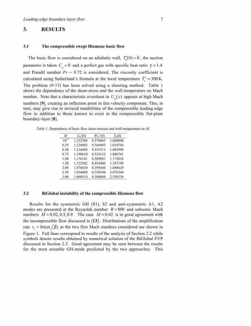
∗ = 300 K.The problem (9-13) has been solved using a shooting method. Table 1shows the dependence of the shear-stress and the wall-temperature on Machnumber. Note that a characteristic overshoot in U0 ( y) appears at high Machnumbers [9], creating an inflection point in this velocity component. This, inturn, may give rise to inviscid instabilities of the compressible leading-edgeflow in addition to those known to exist in the compressible flat-plateboundary-layer [8].

Table 1. Dependence of basic flow shear-stresses and wall-temperature on M.

M U0′(0) W0′ (0) T0(0)10-5 1.232588 0.570465 1.0000000.25 1.228483 0.566095 1.0107460.50 1.216689 0.553511 1.0429900.75 1.198610 0.534132 1.0967411.00 1.176141 0.509881 1.1720161.50 1.125582 0.454480 1.3871982.00 1.076630 0.399360 1.6886292.50 1.034609 0.350344 2.0763443.00 1.000514 0.308888 2.550336

3.2 BiGlobal instability of the compressible Hiemenz flow

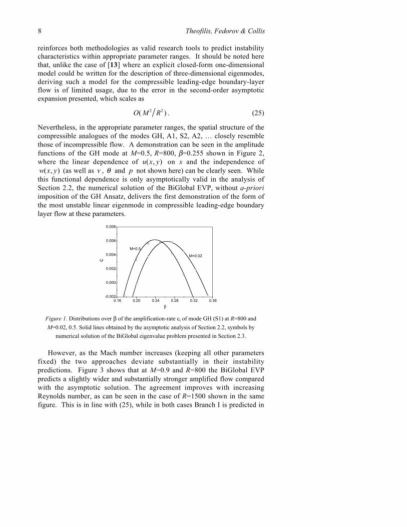
Results for the symmetric GH (S1), S2 and anti-symmetric A1, A2modes are presented at the Reynolds number R = 800 and subsonic Machnumbers M = 0.02, 0.5, 0.9 . The case M = 0.02 is in good agreement withthe incompressible flow discussed in [13]. Distributions of the amplificationrate ci = Im(ω i β) at the two first Mach numbers considered are shown inFigure 1. Full lines correspond to results of the analysis of Section 2.2 whilesymbols denote results obtained by numerical solution of the BiGlobal EVPdiscussed in Section 2.3. Good agreement may be seen between the resultsfor the most unstable GH-mode predicted by the two approaches. This


reinforces both methodologies as valid research tools to predict instabilitycharacteristics within appropriate parameter ranges. It should be noted herethat, unlike the case of [13] where an explicit closed-form one-dimensionalmodel could be written for the description of three-dimensional eigenmodes,deriving such a model for the compressible leading-edge boundary-layerflow is of limited usage, due to the error in the second-order asymptoticexpansion presented, which scales as

O( M 2 R2 ) . (25)

Nevertheless, in the appropriate parameter ranges, the spatial structure of thecompressible analogues of the modes GH, A1, S2, A2, … closely resemblethose of incompressible flow. A demonstration can be seen in the amplitudefunctions of the GH mode at M=0.5, R=800, β=0.255 shown in Figure 2,where the linear dependence of u(x, y) on x and the independence of

w(x, y) (as well as v , θ and p not shown here) can be clearly seen. Whilethis functional dependence is only asymptotically valid in the analysis ofSection 2.2, the numerical solution of the BiGlobal EVP, without a-prioriimposition of the GH Ansatz, delivers the first demonstration of the form ofthe most unstable linear eigenmode in compressible leading-edge boundarylayer flow at these parameters.

0.16 0.20 0.24 0.28 0.32 0.36-0.002

0.000

0.002

0.004

0.006

0.008

M=0.5

M=0.02

Ci

β

Figure 1. Distributions over β of the amplification-rate ci of mode GH (S1) at R=800 andM=0.02, 0.5. Solid lines obtained by the asymptotic analysis of Section 2.2, symbols by

numerical solution of the BiGlobal eigenvalue problem presented in Section 2.3.

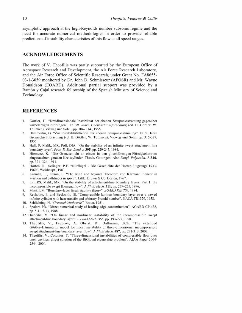
However, as the Mach number increases (keeping all other parametersfixed) the two approaches deviate substantially in their instabilitypredictions. Figure 3 shows that at M=0.9 and R=800 the BiGlobal EVPpredicts a slightly wider and substantially stronger amplified flow comparedwith the asymptotic solution. The agreement improves with increasingReynolds number, as can be seen in the case of R=1500 shown in the samefigure. This is in line with (25), while in both cases Branch I is predicted in


a consistent manner. Work is currently underway to identify the stabilityboundaries using both approaches.

Figure 2. Amplitude functions of the disturbance velocity components of the leadingeigenmode at R = 800, β = 0.255, M = 0.5. Left: u(x,y), Right: w(x,y).

0.08 0.12 0.16 0.20 0.24 0.28 0.32

-0.005

0.000

0.005

0.010

0.015

0.020

R=800

R=1500

M=0.9

Ci

β

GH (S1) A1 S2 A2

Figure 3. Dependence of ci on β for modes GH, A1, S2, A2 at M=0.9, R=800 and 1500.

4. DISCUSSION

The first BiGlobal instability analysis of viscous compressible sweptHiemenz flow has been performed. Good agreement between asymptoticanalysis and numerical solution of the partial-differential eigenvalueproblem has been obtained within appropriate parameter ranges. It has beendemonstrated that the three-dimensional “polynomial” eigenmodes ofincompressible flow [13] persist in the subsonic flow regime. However,differences of the two approaches are found to occur at moderate Reynoldsand high Mach numbers. This underlines both the efficiency of the


asymptotic approach at the high-Reynolds number subsonic regime and theneed for accurate numerical methodologies in order to provide reliablepredictions of instability characteristics of this flow at all speed ranges.

ACKNOWLEDGEMENTS

The work of V. Theofilis was partly supported by the European Office ofAerospace Research and Development, the Air Force Research Laboratory,and the Air Force Office of Scientific Research, under Grant No. FA8655-03-1-3059 monitored by Dr. John D. Schmisseur (AFOSR) and Mr. WayneDonaldson (EOARD). Additional partial support was provided by aRamón y Cajal research fellowship of the Spanish Ministry of Science andTechnology.

REFERENCES

1. Görtler, H. “Dreidimensionale Instabilität der ebenen Staupunktströmung gegenüberwirbelartigen Störungen”. In 50 Jahre Grenzschichtforschung (ed. H. Görtler, W.Tollmien), Vieweg und Sohn., pp. 304- 314., 1955.

2. Hämmerlin, G. “Zur instabilitätstheorie der ebenen Staupunktströmung”. In 50 JahreGrenzschichtforschung (ed. H. Görtler, W. Tollmien), Vieweg und Sohn, pp. 315-327,1955.

3. Hall, P, Malik, MR, Poll, DIA. “On the stability of an infinite swept attachment-lineboundary layer”. Proc. R. Soc. Lond. A 395, pp. 229-245, 1984.

4. Hiemenz, K. “Die Grenzschicht an einem in den gliechförmigen Flüssigkeitsstromeingetauchten geraden Kreiszylinder. Thesis, Göttingen. Also Dingl. Polytechn. J. 326,pp. 321- 324, 1911.

5. Horten, R., Selinger, P.F. “Nurflügel - Die Geschichte der Horten-Flugzeuge 1933-1960”. Weishaupt., 1983.

6. Kármán, T., Edson, L. “The wind and beyond. Theodore von Kármán: Pioneer inaviation and pathfinder in space”. Little, Brown & Co. Boston, 1967.

7. Lin, RS, Malik, MR. “On the stability of attachment-line boundary layers. Part 1. theincompressible swept Hiemenz flow”. J. Fluid Mech. 311, pp. 239–255, 1996.

8. Mack, LM. “Boundary-layer linear stability theory”. AGARD Rep 709, 1984.9. Reshotko, E. and Beckwith, IE. “Compressible laminar boundary layer over a yawed

infinite cylinder with heat-transfer and arbitrary Prandtl number”. NACA TR1379, 1958.10. Schlichting, H. “Grenzschichttheorie”, Braun, 1951.11. Spalart, PR. “Direct numerical study of leading-edge contamination”. AGARD CP-438,

pp. 5-1 - 5-13, 1988.12. Theofilis, V. “On linear and nonlinear instability of the incompressible swept

attachment-line boundary layer”. J. Fluid Mech. 355, pp. 193-227, 1998.13. Theofilis, V., Fedorov, A. Obrist, D., Dallmann, UCh. “The extended

Görtler–Hämmerlin model for linear instability of three-dimensional incompressibleswept attachment-line boundary layer flow”. J. Fluid Mech. 487, pp. 271-313, 2003.

14. Theofilis, V., Colonius, T. “Three-dimensional instabilities of compressible flow overopen cavities: direct solution of the BiGlobal eigenvalue problem”. AIAA Paper 2004-2544, 2004.

leading-edge boundary layer flow prandtl’s … · numerical solution of the appropriate...

Documents