lean vs. six sigma -asq handout - ascendantconsulting.netascendantconsulting.net/ftpdocs/pdfs/lean...
TRANSCRIPT
1
Informational
Brief
2012, All Rights Reserved
Lean vs. Six SigmaLean vs. Six Sigma(a Case Study)(a Case Study)
� Introduction
� Background
� Case Study
� The Dice Experiment (opt.)
“Let the flow manage the processes, and not letmanagement manage the flow” Taiichi Ohno
Presenter: Ken Myers, CQE, CSSBB, CMBB, PBSLPresident, Ascendant Consulting Service, Inc.
2
Lean vs. Six Sigma Slide 2
Observations
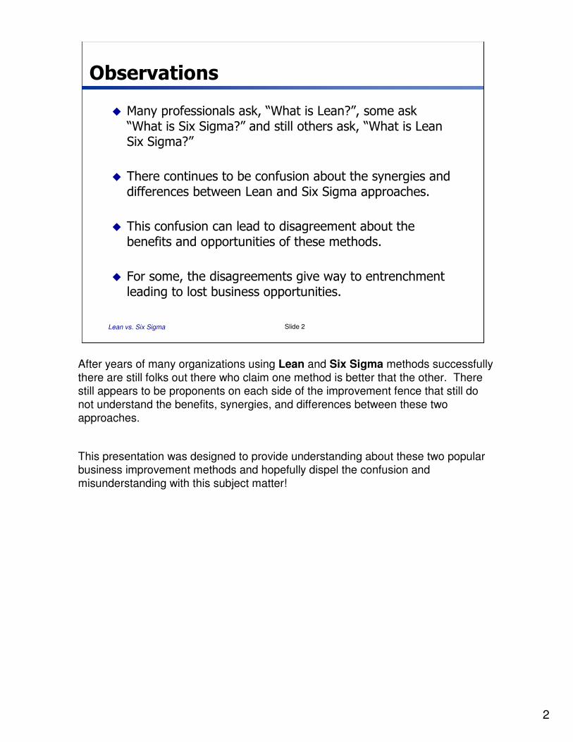
� Many professionals ask, “What is Lean?”, some ask “What is Six Sigma?” and still others ask, “What is Lean Six Sigma?”
� There continues to be confusion about the synergies and differences between Lean and Six Sigma approaches.
� This confusion can lead to disagreement about the benefits and opportunities of these methods.
� For some, the disagreements give way to entrenchment leading to lost business opportunities.
After years of many organizations using Lean and Six Sigma methods successfully there are still folks out there who claim one method is better that the other. There still appears to be proponents on each side of the improvement fence that still do not understand the benefits, synergies, and differences between these two approaches.
This presentation was designed to provide understanding about these two popular business improvement methods and hopefully dispel the confusion and misunderstanding with this subject matter!
3
Lean vs. Six Sigma Slide 3
Discussion Coverage
� Provide some background on Lean and Six Sigma.
� Present a Case Study where Lean and Six Sigma approaches were used together.
� If time, show a simulation illustrating the relationship between production flow and process variation.
4
InformationalBrief
2012, All Rights Reserved
BackgroundBackground
“Improvement means the organized creation of beneficial change, and the attainment of unprecedented levels of performance. A synonym is breakthrough.” J. Juran
5
Lean vs. Six Sigma Slide 5
TPS* and North American Lean
� Lean began in 1985 with the establishment of the International Motor Vehicle Program (IMVP) at MIT under Daniel Roos.
� It was supported by over 50 sponsoring organizations across the world interested in understanding TPS.
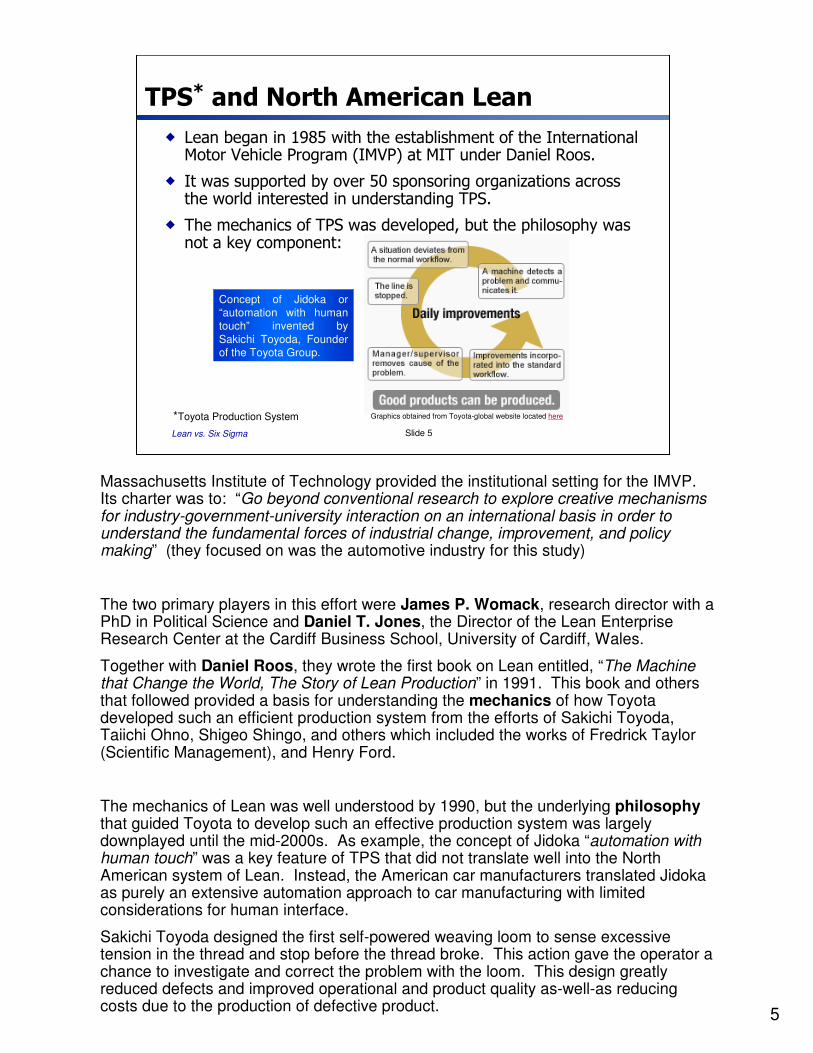
� The mechanics of TPS was developed, but the philosophy was not a key component:
Concept of Jidoka or “automation with human touch” invented by Sakichi Toyoda, Founder of the Toyota Group.
Graphics obtained from Toyota-global website located here*Toyota Production System
Massachusetts Institute of Technology provided the institutional setting for the IMVP. Its charter was to: “Go beyond conventional research to explore creative mechanisms for industry-government-university interaction on an international basis in order to understand the fundamental forces of industrial change, improvement, and policy making” (they focused on was the automotive industry for this study)
The two primary players in this effort were James P. Womack, research director with a PhD in Political Science and Daniel T. Jones, the Director of the Lean Enterprise Research Center at the Cardiff Business School, University of Cardiff, Wales.
Together with Daniel Roos, they wrote the first book on Lean entitled, “The Machine that Change the World, The Story of Lean Production” in 1991. This book and others that followed provided a basis for understanding the mechanics of how Toyota developed such an efficient production system from the efforts of Sakichi Toyoda, Taiichi Ohno, Shigeo Shingo, and others which included the works of Fredrick Taylor (Scientific Management), and Henry Ford.
The mechanics of Lean was well understood by 1990, but the underlying philosophythat guided Toyota to develop such an effective production system was largely downplayed until the mid-2000s. As example, the concept of Jidoka “automation with human touch” was a key feature of TPS that did not translate well into the North American system of Lean. Instead, the American car manufacturers translated Jidoka as purely an extensive automation approach to car manufacturing with limited considerations for human interface.
Sakichi Toyoda designed the first self-powered weaving loom to sense excessive tension in the thread and stop before the thread broke. This action gave the operator a chance to investigate and correct the problem with the loom. This design greatly reduced defects and improved operational and product quality as-well-as reducing costs due to the production of defective product.
6
Lean vs. Six Sigma Slide 6
Lean Principles – LEI Perspective*
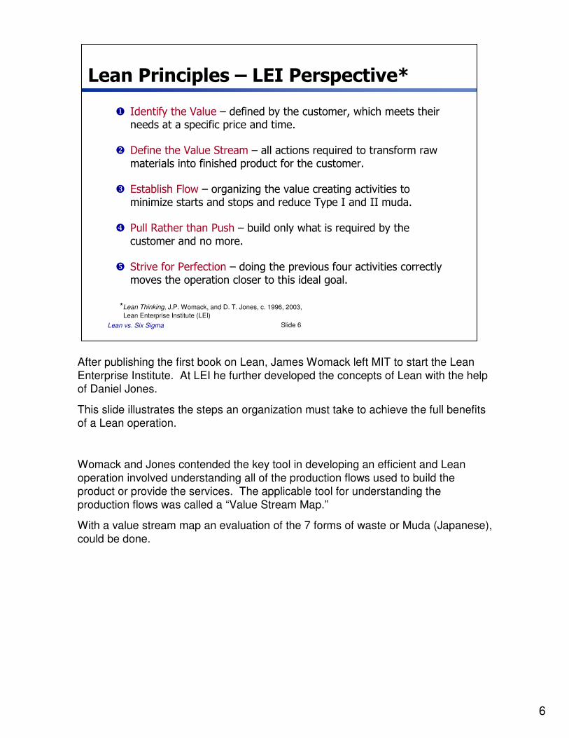
� Identify the Value – defined by the customer, which meets their needs at a specific price and time.
� Define the Value Stream – all actions required to transform raw materials into finished product for the customer.
� Establish Flow – organizing the value creating activities to minimize starts and stops and reduce Type I and II muda.
� Pull Rather than Push – build only what is required by the customer and no more.
� Strive for Perfection – doing the previous four activities correctly moves the operation closer to this ideal goal.
*Lean Thinking, J.P. Womack, and D. T. Jones, c. 1996, 2003,
Lean Enterprise Institute (LEI)
After publishing the first book on Lean, James Womack left MIT to start the Lean Enterprise Institute. At LEI he further developed the concepts of Lean with the help of Daniel Jones.
This slide illustrates the steps an organization must take to achieve the full benefits of a Lean operation.
Womack and Jones contended the key tool in developing an efficient and Lean operation involved understanding all of the production flows used to build the product or provide the services. The applicable tool for understanding the production flows was called a “Value Stream Map.”
With a value stream map an evaluation of the 7 forms of waste or Muda (Japanese), could be done.
7
Lean vs. Six Sigma Slide 7
Primary Tool:
Value Stream Map
InformationFlow
Work and/or Material Flow
3 days
Suppliers
6-week
Forecast
3 m 1 m4 m
2.3 d
1.2 m 1.2 m 1.1 m
1.7 d
VA
NVA13.5 days
11.5 min
WeeklyFAX
WeeklyFAX
CustomerCustomer
6.1 d 2 d 1.4 d
Production Control
Production Control
II
RawStock
4 days
MRP
C/T = 1.2 m
C/Tv = 0.6 m
C/O = 0ER = 3.5%
Labeling
& Packaging
C/T = 4 m
C/Tv = 2 m
C/O = 0.5 mYield = 97%
Shaping
C/T = 1.2 m
C/Tv = 0.3 mC/O = 2 m
Scrap = 12%
TestingAssembly
C/T = 1 mC/Tv = 2.2 m
C/O = 5 m
Scrap = 2%
1 Operator
C/T = 3 m
C/Tv = 0.7 m
C/O = 45 mYield = 87%
Forming Shipping
C/T = 1.1 mC/Tv = 0.2 m
C/O = 0
ER = 0.3%
2 Operators 1 Operator 1 Operator 2 Operators 2 Operators
A-1200
B-2200C-1850
I I I I I
A-2600
B-1400
C-1500
10,244
5 d
21,013
10 d
29,564
14 dC/T = 1.2 m
C/Tv = 0.6 m
C/O = 0ER = 3.5%
Labeling
& Packaging
C/T = 4 m
C/Tv = 2 m
C/O = 0.5 mYield = 97%
Shaping
C/T = 1.2 m
C/Tv = 0.3 mC/O = 2 m
Scrap = 12%
TestingAssembly
C/T = 1 mC/Tv = 2.2 m
C/O = 5 m
Scrap = 2%
1 Operator
C/T = 3 m
C/Tv = 0.7 m
C/O = 45 mYield = 87%
Forming Shipping
C/T = 1.1 mC/Tv = 0.2 m
C/O = 0
ER = 0.3%
2 Operators 1 Operator 1 Operator 2 Operators 2 Operators
A-1200
B-2200C-1850
II II II II II
A-2600
B-1400
C-1500
10,244
5 d
21,013
10 d
29,564
14 d
Weekly Schedule
Dist Centers
30/60/90 day
Forecasts
Daily
Order
Daily
Order
II
II
II
Daily ShipSchedule
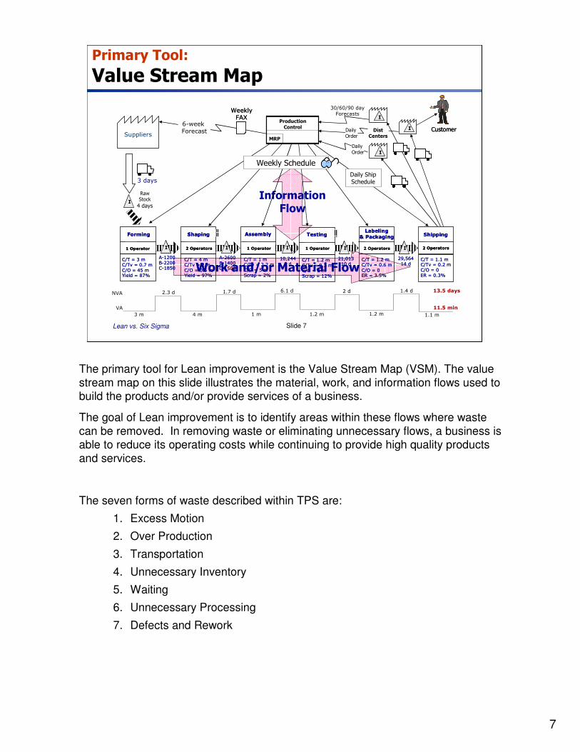
The primary tool for Lean improvement is the Value Stream Map (VSM). The value stream map on this slide illustrates the material, work, and information flows used to build the products and/or provide services of a business.
The goal of Lean improvement is to identify areas within these flows where waste can be removed. In removing waste or eliminating unnecessary flows, a business is able to reduce its operating costs while continuing to provide high quality products and services.
The seven forms of waste described within TPS are:
1. Excess Motion
2. Over Production
3. Transportation
4. Unnecessary Inventory
5. Waiting
6. Unnecessary Processing
7. Defects and Rework
8
Lean vs. Six Sigma Slide 8
Lean is About Managing Flows
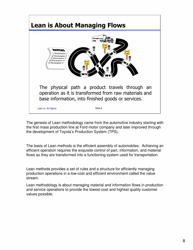
The physical path a product travels through an operation as it is transformed from raw materials and base information, into finished goods or services.
Time Time
TrapTrapTime Time
TrapTrap
Time Time
TrapTrapTime Time
TrapTrap
Time Time
TrapTrapTime Time
TrapTrap
The genesis of Lean methodology came from the automotive industry starting with the first mass production line at Ford motor company and later improved through the development of Toyota’s Production System (TPS).
The basis of Lean methods is the efficient assembly of automobiles. Achieving an efficient operation requires the exquisite control of part, information, and material flows as they are transformed into a functioning system used for transportation.
Lean methods provides a set of rules and a structure for efficiently managing production operations in a low-cost and efficient environment called the value stream.
Lean methodology is about managing material and information flows in production and service operations to provide the lowest-cost and highest quality customer values possible.
9
Lean vs. Six Sigma Slide 9
Work-Flow Measures
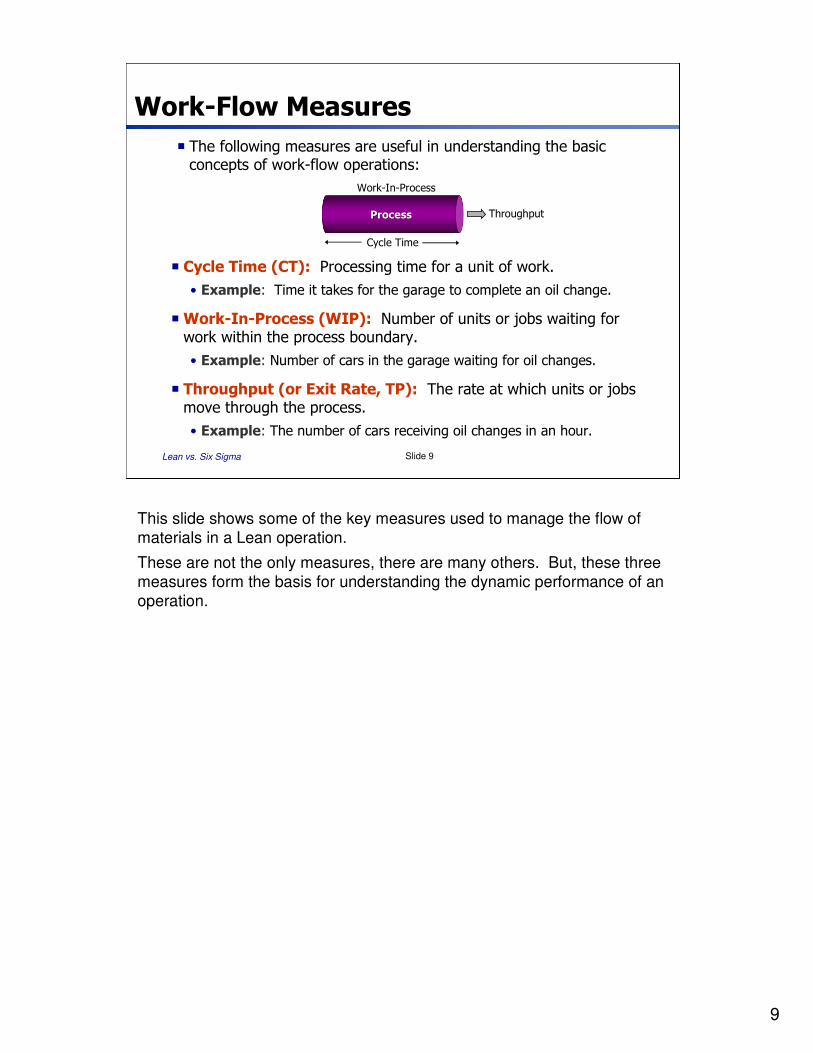
� The following measures are useful in understanding the basic concepts of work-flow operations:
ProcessProcess
Work-In-Process
Throughput
Cycle Time
� Cycle Time (CT): Processing time for a unit of work.
• Example: Time it takes for the garage to complete an oil change.
�Work-In-Process (WIP): Number of units or jobs waiting for work within the process boundary.
• Example: Number of cars in the garage waiting for oil changes.
� Throughput (or Exit Rate, TP): The rate at which units or jobs move through the process.
• Example: The number of cars receiving oil changes in an hour.
This slide shows some of the key measures used to manage the flow of materials in a Lean operation.
These are not the only measures, there are many others. But, these three measures form the basis for understanding the dynamic performance of an operation.

10
Lean vs. Six Sigma Slide 10
Relationships:
Little's Law of System Flow*
� Describes the relationship between WIP, CT, and TP in a steady-state process having predictable controls.
� It is calculated as:
WIP
TP CT
WIP = # of units
CT = time
TP = (# of units)/time Prof. John D.C. Little
CT
WIPTP =
*Factory Physics, 3rd Ed., 2008, 2001, 1999, 1995, p. 518
Expression as fundamental as Newton’s 2nd Law of Motion
Little's law is the most fundamental queuing relationship known to man. It describes the relationship between the Work in Progress (WIP), Throughput (TP), and Cycle Time (CT). It is considered as fundamental for understanding operational management as Newton’s 2nd law of motion is to understanding universal motion. However, there is a distinction between these two expressions. That distinction is that in Little’s Law all of the members of the expression are variables. There are no constants. Therefore, in order to establish a workable expression, one of the variables is forced as a constant.
In the Toyota Production System WIP is selected as the constant. WIP is designated constant within the signaling structure called a “Kanban.” Using constant WIP stabilizes the flows and makes them predictable. In this framework Little’s law can then be used to predict TP given CT, or vice-versa.
Despite its great usefulness, there is a limitation with Little’s law. It does not account for time and/or flow variations in operational systems. In order to understand the effects of variation on the operation a second law called the VUT formula is used.
The reference provided at the bottom of the page, “Factory Physics” includes details on the VUT formula which relates system variability, V, to the system utilization, U, to the average processing time of a station, T, with the wait time, WT, in the expression:
WT = V * U * T. Little’s law and the VUT formula are fundamental relationships in queuing theory and operations research.
11
Lean vs. Six Sigma Slide 11
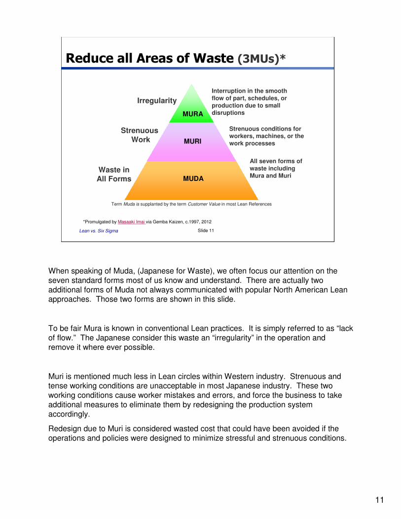
Reduce all Areas of Waste (3MUs)*
MURA
MURI
MUDA
Irregularity
Strenuous
Work
Waste inAll Forms
Interruption in the smooth
flow of part, schedules, or
production due to smalldisruptions
Strenuous conditions for workers, machines, or the
work processes
All seven forms of
waste including Mura and Muri
Term Muda is supplanted by the term Customer Value in most Lean References
*Promulgated by Masaaki Imai via Gemba Kaizen, c.1997, 2012
When speaking of Muda, (Japanese for Waste), we often focus our attention on the seven standard forms most of us know and understand. There are actually two additional forms of Muda not always communicated with popular North American Lean approaches. Those two forms are shown in this slide.
To be fair Mura is known in conventional Lean practices. It is simply referred to as “lack of flow.” The Japanese consider this waste an “irregularity” in the operation and remove it where ever possible.
Muri is mentioned much less in Lean circles within Western industry. Strenuous and tense working conditions are unacceptable in most Japanese industry. These two working conditions cause worker mistakes and errors, and force the business to take additional measures to eliminate them by redesigning the production system accordingly.
Redesign due to Muri is considered wasted cost that could have been avoided if the operations and policies were designed to minimize stressful and strenuous conditions.
12
Lean vs. Six Sigma Slide 12
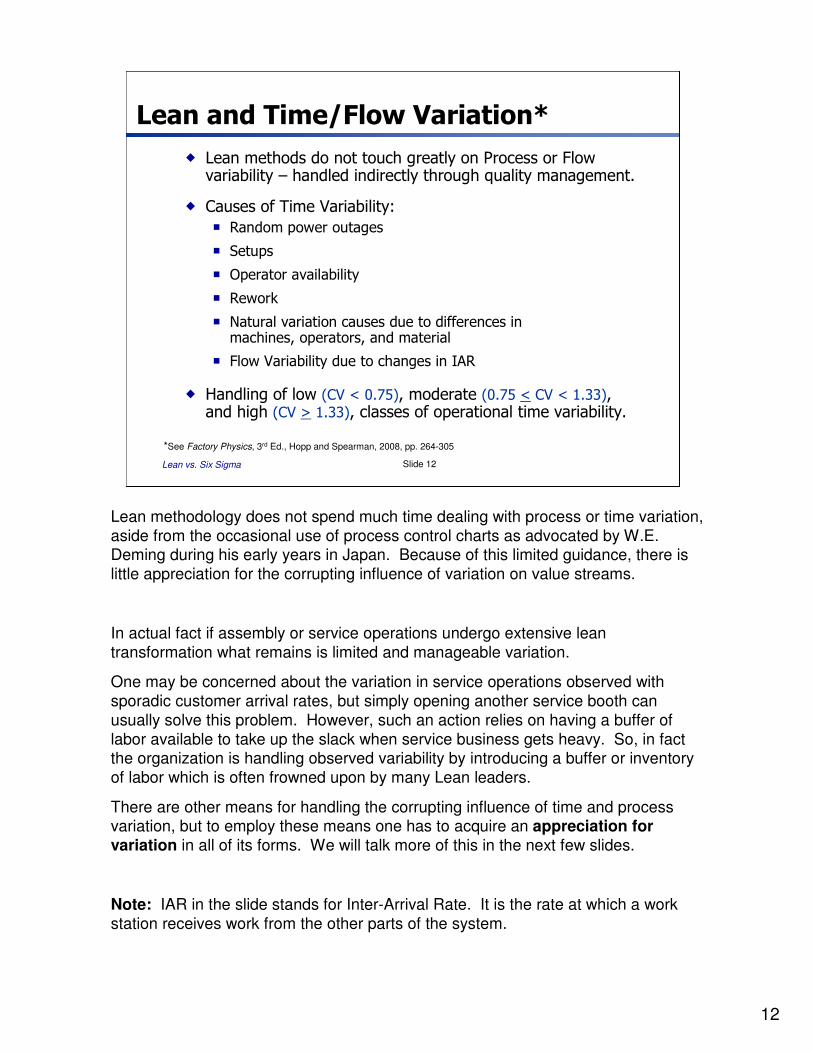
Lean and Time/Flow Variation*
� Lean methods do not touch greatly on Process or Flow variability – handled indirectly through quality management.
� Causes of Time Variability:
� Random power outages
� Setups
� Operator availability
� Rework
� Natural variation causes due to differences in machines, operators, and material
� Flow Variability due to changes in IAR
� Handling of low (CV < 0.75), moderate (0.75 < CV < 1.33), and high (CV > 1.33), classes of operational time variability.
*See Factory Physics, 3rd Ed., Hopp and Spearman, 2008, pp. 264-305
Lean methodology does not spend much time dealing with process or time variation, aside from the occasional use of process control charts as advocated by W.E. Deming during his early years in Japan. Because of this limited guidance, there is little appreciation for the corrupting influence of variation on value streams.
In actual fact if assembly or service operations undergo extensive lean transformation what remains is limited and manageable variation.
One may be concerned about the variation in service operations observed with sporadic customer arrival rates, but simply opening another service booth can usually solve this problem. However, such an action relies on having a buffer of labor available to take up the slack when service business gets heavy. So, in fact the organization is handling observed variability by introducing a buffer or inventory of labor which is often frowned upon by many Lean leaders.
There are other means for handling the corrupting influence of time and process variation, but to employ these means one has to acquire an appreciation for variation in all of its forms. We will talk more of this in the next few slides.
Note: IAR in the slide stands for Inter-Arrival Rate. It is the rate at which a work station receives work from the other parts of the system.
13
Lean vs. Six Sigma Slide 13
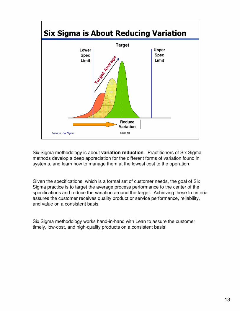
Six Sigma is About Reducing Variation
Target Average
ReduceVariation
TargetUpper
Spec
Limit
Lower
Spec
Limit
Six Sigma methodology is about variation reduction. Practitioners of Six Sigma methods develop a deep appreciation for the different forms of variation found in systems, and learn how to manage them at the lowest cost to the operation.
Given the specifications, which is a formal set of customer needs, the goal of Six Sigma practice is to target the average process performance to the center of the specifications and reduce the variation around the target. Achieving these to criteria assures the customer receives quality product or service performance, reliability, and value on a consistent basis.
Six Sigma methodology works hand-in-hand with Lean to assure the customer timely, low-cost, and high-quality products on a consistent basis!
14
Lean vs. Six Sigma Slide 14
Measuring Process Quality
LSL USL
σσσσ
LSLLSL USLUSL
σσσσσσσσ
+3σσσσ-3σσσσ
3-Sigma Quality <10% Defects(Considered good
quality 20 years ago...)
LSL USL
σσσσ
LSL USL
σσσσσσσσ
+4σσσσ-4σσσσ
4-Sigma Quality <1% Defects(Considered good quality today...)
LSL USL
σσσσ
LSL USL
σσσσσσσσ
+6σσσσ-6σσσσ
6-Sigma Quality <0.01% Defects(Considered world-class
quality today!)
OperatingWindow
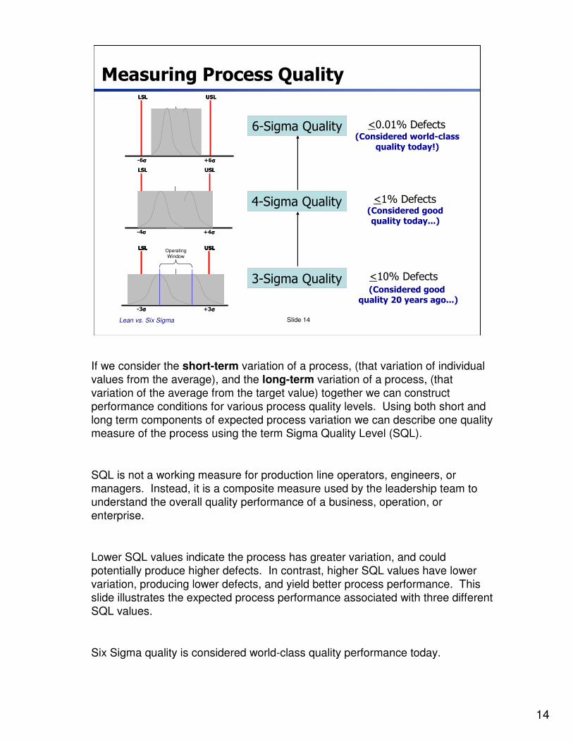
If we consider the short-term variation of a process, (that variation of individual values from the average), and the long-term variation of a process, (that variation of the average from the target value) together we can construct performance conditions for various process quality levels. Using both short and long term components of expected process variation we can describe one quality measure of the process using the term Sigma Quality Level (SQL).
SQL is not a working measure for production line operators, engineers, or managers. Instead, it is a composite measure used by the leadership team to understand the overall quality performance of a business, operation, or enterprise.
Lower SQL values indicate the process has greater variation, and could potentially produce higher defects. In contrast, higher SQL values have lower variation, producing lower defects, and yield better process performance. This slide illustrates the expected process performance associated with three different SQL values.
Six Sigma quality is considered world-class quality performance today.
15
Lean vs. Six Sigma Slide 15
Improving Customer Value
LO
S
S
$20
$0
Bad
Product
Bad
Product
$10
Good
Product
UpperUpper
SpecSpecLowerLower
SpecSpec
Greater VariationProduces
Greater Loss
LO
S
S
LO
S
S
$20
$0
Bad
Product
Bad
Product
$10
Good
Product
Good
Product
UpperUpper
SpecSpecLowerLower
SpecSpec
Greater VariationProduces
Greater Loss
L
O
S
S
$20
$0
Bad
Product
Bad
Product
$10
Closerto
Target
UpperUpper
SpecSpecLowerLower
SpecSpec
Lower VariationMinimizes Loss
L
O
S
S
L
O
S
S
$20
$0
Bad
Product
Bad
Product
$10
Closerto
Target
Closerto
Target
UpperUpper
SpecSpecLowerLower
SpecSpec
Lower VariationMinimizes Loss
Taguchi's Loss
Function
Provides greater performance consistency which improves value …
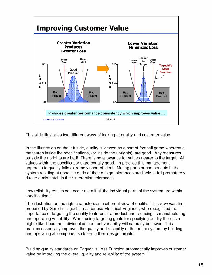
This slide illustrates two different ways of looking at quality and customer value.
In the illustration on the left side, quality is viewed as a sort of football game whereby all measures inside the specifications, (or inside the uprights), are good. Any measures outside the uprights are bad! There is no allowance for values nearer to the target. All values within the specifications are equally good. In practice this management approach to quality falls extremely short of ideal. Mating parts or components in the system residing at opposite ends of their design tolerances are likely to fail prematurely due to a mismatch in their interaction tolerances.
Low reliability results can occur even if all the individual parts of the system are within specifications.
The illustration on the right characterizes a different view of quality. This view was first proposed by Genichi Taguchi, a Japanese Electrical Engineer, who recognized the importance of targeting the quality features of a product and reducing its manufacturing and operating variability. When using targeting goals for specifying quality there is a higher likelihood the individual component variability will naturally be lower. This practice essentially improves the quality and reliability of the entire system by building and operating all components closer to their design targets.
Building quality standards on Taguchi’s Loss Function automatically improves customer value by improving the overall quality and reliability of the system.
16
Lean vs. Six Sigma Slide 16
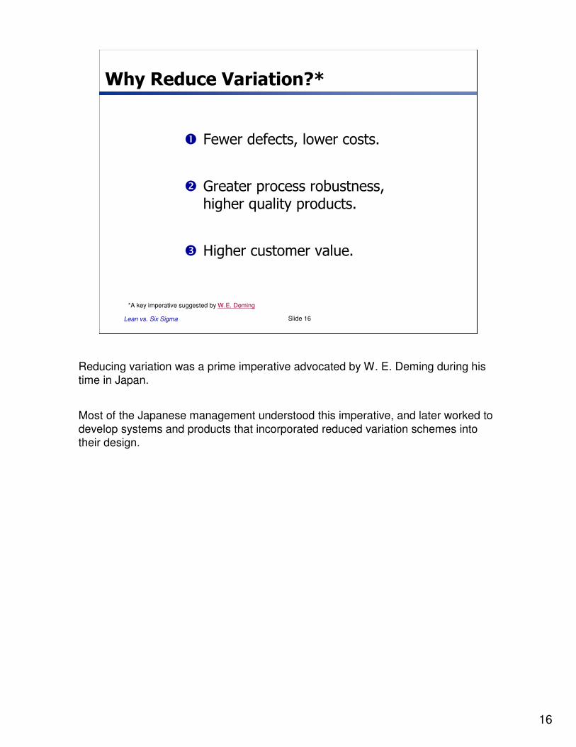
Why Reduce Variation?*
� Fewer defects, lower costs.
� Greater process robustness, higher quality products.
� Higher customer value.
*A key imperative suggested by W.E. Deming
Reducing variation was a prime imperative advocated by W. E. Deming during his time in Japan.
Most of the Japanese management understood this imperative, and later worked to develop systems and products that incorporated reduced variation schemes into their design.

17
Lean vs. Six Sigma Slide 17
A System of Improvement
Low HighSystem or Problem Complexity
• Spaghetti Diagrams
• Value Stream Mapping
• Takt Time
• Kanban
• One-Piece Flow
• Material Flow Layout
• Setup Reduction
• Total Productive Maintenance
Kaizen• Workplace Org - 5S• Process Mapping• Mistake Proofing• Standard Work• Cause & Effect Diagram• Brainstorming Tools• 5-Whys Evaluation• Pareto Charts• Force Field Analysis• Check Sheets
Lean• DMAIC Approach• Capability Studies • MSA/Gage R&R Studies• ANOVA/ANOM• Statistical Tests• Design of Experiments• Regression Analysis• Box Plots• Tolerance Analysis• Process Control Plans
Six Sigma
• Waste Reduction
• Work Standardization
• Flow Improvement
• Change of Paradigm
• Mistake Elimination
• Foundation for Lean
• Improve Speed & C-T
• NVA Reduction
• Waste Reduction
• Inventory Turns
• Balanced Product Flow
• Lead-time Reliability
• Variance Reduction
• Process Stability
• Process Capability
• Robust Tolerancing
• Yield Improvement
• Defect Prevention
Leadership, Creativity, InnovationLeadership, Creativity, Innovation
Total Employee InvolvementTotal Employee Involvement
ToolsetToolset
ImprovementImprovement
FocusFocus
PerformancePerformance
Metrics andMetrics and
ProcessProcess
FeedbackFeedback
Adapted from iSixSigma.com
In most “Transfer” operations, (operations where much of the value is obtained by moving the product through multiple stages or steps), both process complexity and variation are moderate to low. In these operations, straightforward methods of efficiency improvement using Industrial Engineering approaches are appropriate. Improving system flow is comparable to improving the manufacturing or service process. The use of Kaizen and Lean in these systems usually provides ample tools to solve most of the problems and provide effective improvement to these systems. This is the case in 70-80% of the manufacturing and service operations in existence, and hence the success of Lean methodology.
In about 10-20% of manufacturing systems value is created in isolated locations within the value stream. These systems are called “Complex Stationary” operations. In these operations, the manufacturer is required to obtain a high level of process understanding to create product value. Examples of such operations are: Chemical, Microelectronic, Pharmaceutical, and Metallurgical manufacturing as well as Agriculture and Farming applications. These operations are more complex and prone to greater process variation than “Transfer” operations.
Complex Stationary operations require us to develop additional understanding of the system of manufacture over the basic flow, timing, and capacity characteristics. In addition, we also need to know how the input variables in these processes need to be configured to yield the highest possible product performance and quality. The Six Sigma tool box provides us with an ability to meet the needs of these processes. So, it’s not an either or situation with Kaizen, Lean, and Six Sigma; it’s a when to use situation!
18
InformationalBrief
2012, All Rights Reserved
Case StudyCase Study
“Understanding variation is key to successin quality and business” W. E. Deming
19
Lean vs. Six Sigma Slide 19
The Unit of Work and Process
Separation
Discarded Cells
Final Product
GrowthMedia
WorkingCells
2L MiniFerm
Unit of Work
DO = Dissolved Oxygen
pH = acidity level
Low High
pH Probe
DO Probe
Fermentation
Experimental Pilot Plant Operations
All process andresults Data
Actual Work Product
Raw MaterialPurification
ChromatographyProcess
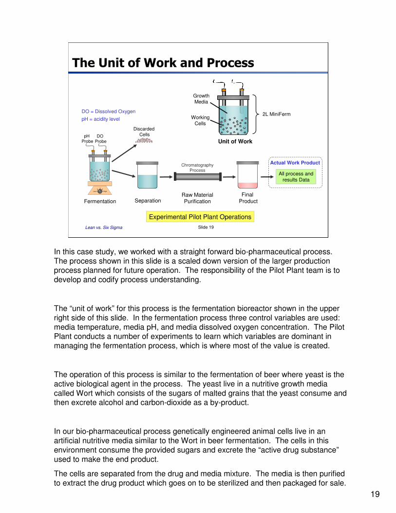
In this case study, we worked with a straight forward bio-pharmaceutical process. The process shown in this slide is a scaled down version of the larger production process planned for future operation. The responsibility of the Pilot Plant team is to develop and codify process understanding.
The “unit of work” for this process is the fermentation bioreactor shown in the upper right side of this slide. In the fermentation process three control variables are used: media temperature, media pH, and media dissolved oxygen concentration. The Pilot Plant conducts a number of experiments to learn which variables are dominant in managing the fermentation process, which is where most of the value is created.
The operation of this process is similar to the fermentation of beer where yeast is the active biological agent in the process. The yeast live in a nutritive growth media called Wort which consists of the sugars of malted grains that the yeast consume and then excrete alcohol and carbon-dioxide as a by-product.
In our bio-pharmaceutical process genetically engineered animal cells live in an artificial nutritive media similar to the Wort in beer fermentation. The cells in this environment consume the provided sugars and excrete the “active drug substance”used to make the end product.
The cells are separated from the drug and media mixture. The media is then purified to extract the drug product which goes on to be sterilized and then packaged for sale.
20
Lean vs. Six Sigma Slide 20
The Problem and Business Case
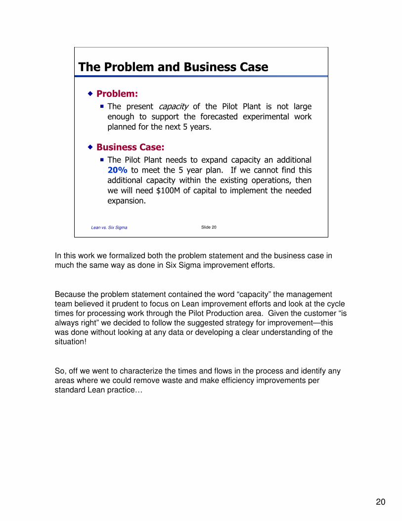
� Problem:
� The present capacity of the Pilot Plant is not large
enough to support the forecasted experimental work
planned for the next 5 years.
� Business Case:
� The Pilot Plant needs to expand capacity an additional
20% to meet the 5 year plan. If we cannot find this
additional capacity within the existing operations, then
we will need $100M of capital to implement the needed
expansion.
In this work we formalized both the problem statement and the business case in much the same way as done in Six Sigma improvement efforts.
Because the problem statement contained the word “capacity” the management team believed it prudent to focus on Lean improvement efforts and look at the cycle times for processing work through the Pilot Production area. Given the customer “is always right” we decided to follow the suggested strategy for improvement—this was done without looking at any data or developing a clear understanding of the situation!
So, off we went to characterize the times and flows in the process and identify any areas where we could remove waste and make efficiency improvements per standard Lean practice…
21
Lean vs. Six Sigma Slide 21
Y8LowLowLowT8
Y7HighLowLowT7
Y6LowHighLowT6
Y5HighHighLowT5
Y4LowLowHighT4
Y3HighLowHighT3
Y2LowHighHighT2
Y1HighHighHighT1
DOpHTemp
Process Yield
Settings for Experimental FactorsTrial
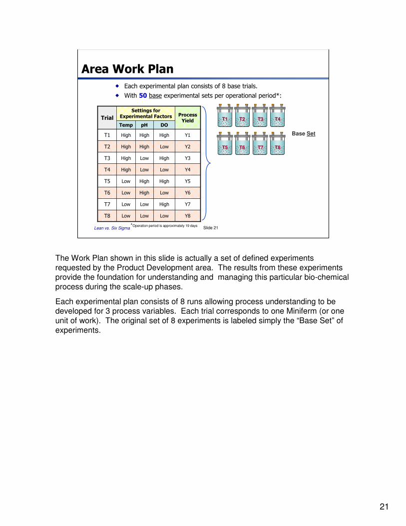
Area Work Plan
� Each experimental plan consists of 8 base trials.
� With 50 base experimental sets per operational period*:
T1T1 T2T2 T3T3 T4T4
T5T5 T6T6 T7T7 T8T8
Base Set
*Operation period is approximately 19 days
The Work Plan shown in this slide is actually a set of defined experiments requested by the Product Development area. The results from these experiments provide the foundation for understanding and managing this particular bio-chemical process during the scale-up phases.
Each experimental plan consists of 8 runs allowing process understanding to be developed for 3 process variables. Each trial corresponds to one Miniferm (or one unit of work). The original set of 8 experiments is labeled simply the “Base Set” of experiments.
22
Lean vs. Six Sigma Slide 22
Y8LowLowLowT8
Y7HighLowLowT7
Y6LowHighLowT6
Y5HighHighLowT5
Y4LowLowHighT4
Y3HighLowHighT3
Y2LowHighHighT2
Y1HighHighHighT1
DOpHTemp
Process Yield
Settings for Experimental FactorsTrial
Experimental Loss
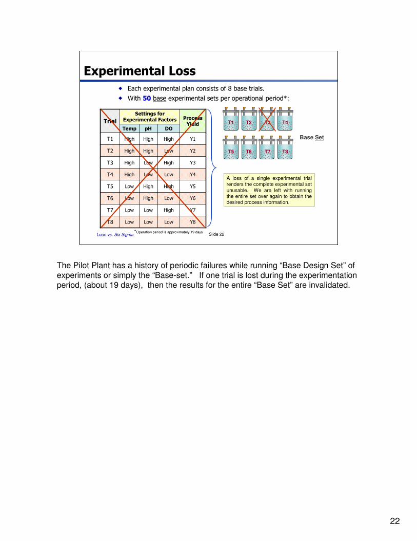
� Each experimental plan consists of 8 base trials.
� With 50 base experimental sets per operational period*:
T1T1 T2T2 T3T3 T4T4
T5T5 T6T6 T7T7 T8T8
Base Set
*Operation period is approximately 19 days
A loss of a single experimental trial renders the complete experimental set unusable. We are left with running the entire set over again to obtain the desired process information.
The Pilot Plant has a history of periodic failures while running “Base Design Set” of experiments or simply the “Base-set.” If one trial is lost during the experimentation period, (about 19 days), then the results for the entire “Base Set” are invalidated.
23
Lean vs. Six Sigma Slide 23
Y8LowLowLowT8
Y7HighLowLowT7
Y6LowHighLowT6
Y5HighHighLowT5
Y4LowLowHighT4
Y3HighLowHighT3
Y2LowHighHighT2
Y1HighHighHighT1
DOpHTemp
Process Yield
Settings for Experimental FactorsTrial
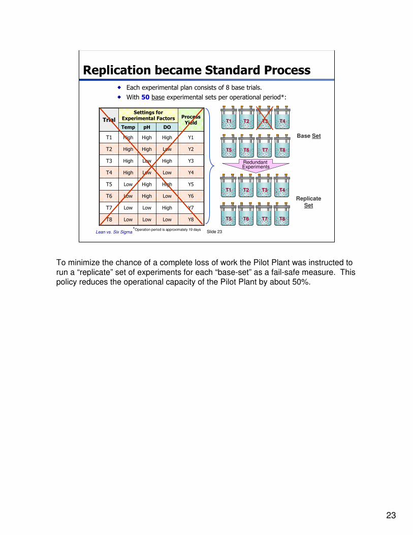
Replication became Standard Process
� Each experimental plan consists of 8 base trials.
� With 50 base experimental sets per operational period*:
T1T1 T2T2 T3T3 T4T4
T5T5 T6T6 T7T7 T8T8
Base Set
T1T1 T2T2 T3T3 T4T4
T5T5 T6T6 T7T7 T8T8
ReplicateSet
Redundant Experiments
*Operation period is approximately 19 days
To minimize the chance of a complete loss of work the Pilot Plant was instructed to run a “replicate” set of experiments for each “base-set” as a fail-safe measure. This policy reduces the operational capacity of the Pilot Plant by about 50%.
24
Lean vs. Six Sigma Slide 24
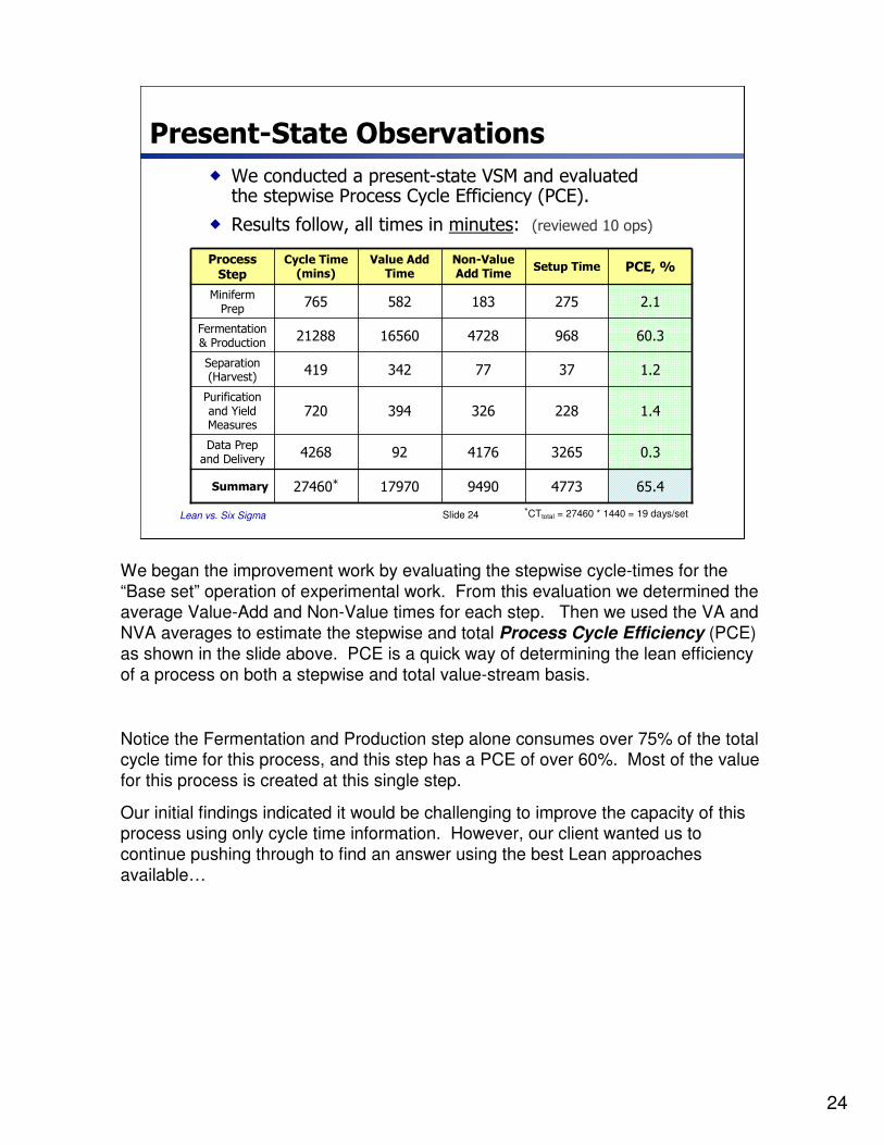
Present-State Observations
� We conducted a present-state VSM and evaluated the stepwise Process Cycle Efficiency (PCE).
� Results follow, all times in minutes: (reviewed 10 ops)
0.332654176924268Data Prep
and Delivery
60.396847281656021288Fermentation & Production
65.4477394901797027460*Summary
1.4228326394720Purification and Yield Measures
1.23777342419Separation(Harvest)
2.1275183582765Miniferm Prep
PCE, %Setup TimeNon-ValueAdd Time
Value AddTime
Cycle Time(mins)
Process Step
*CTtotal = 27460 * 1440 = 19 days/set
We began the improvement work by evaluating the stepwise cycle-times for the “Base set” operation of experimental work. From this evaluation we determined the average Value-Add and Non-Value times for each step. Then we used the VA and NVA averages to estimate the stepwise and total Process Cycle Efficiency (PCE) as shown in the slide above. PCE is a quick way of determining the lean efficiency of a process on both a stepwise and total value-stream basis.
Notice the Fermentation and Production step alone consumes over 75% of the total cycle time for this process, and this step has a PCE of over 60%. Most of the value for this process is created at this single step.
Our initial findings indicated it would be challenging to improve the capacity of this process using only cycle time information. However, our client wanted us to continue pushing through to find an answer using the best Lean approaches available…
25
Lean vs. Six Sigma Slide 25
80%30%Continuous or One Piece Flow Assembly
35%15%Batch Transfer Assembly
50%10%Transactional Processes
25%5%Creative/Cognitive Processes
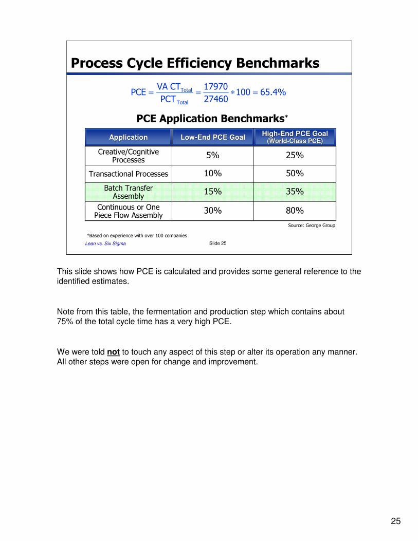
Process Cycle Efficiency Benchmarks
65.4%10027460
17970
PCT
CT VACEP
Total
Total=∗==
PCE Application Benchmarks*
*Based on experience with over 100 companies
ApplicationApplicationHighHigh--End PCE GoalEnd PCE Goal
(World(World--Class PCE)Class PCE)LowLow--End PCE GoalEnd PCE Goal
Source: George Group
This slide shows how PCE is calculated and provides some general reference to the identified estimates.
Note from this table, the fermentation and production step which contains about 75% of the total cycle time has a very high PCE.
We were told not to touch any aspect of this step or alter its operation any manner. All other steps were open for change and improvement.
26
Lean vs. Six Sigma Slide 26
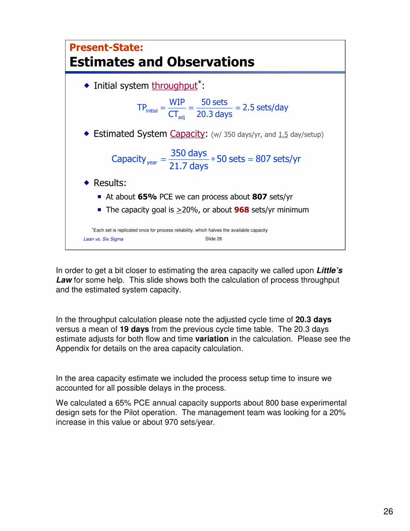
Present-State:
Estimates and Observations
� Initial system throughput*:
sets/day 2.5days 20.3
sets 50
CT
WIPTP
adj
initial ===
*Each set is replicated once for process reliability, which halves the available capacity
� Estimated System Capacity: (w/ 350 days/yr, and 1.5 day/setup)
sets/yr 807sets 50days 21.7
days 350apacityC year =∗=
� Results:
� At about 65% PCE we can process about 807 sets/yr
� The capacity goal is >20%, or about 968 sets/yr minimum
In order to get a bit closer to estimating the area capacity we called upon Little’s Law for some help. This slide shows both the calculation of process throughput and the estimated system capacity.
In the throughput calculation please note the adjusted cycle time of 20.3 daysversus a mean of 19 days from the previous cycle time table. The 20.3 days estimate adjusts for both flow and time variation in the calculation. Please see the Appendix for details on the area capacity calculation.
In the area capacity estimate we included the process setup time to insure we accounted for all possible delays in the process.
We calculated a 65% PCE annual capacity supports about 800 base experimental design sets for the Pilot operation. The management team was looking for a 20% increase in this value or about 970 sets/year.
27
Lean vs. Six Sigma Slide 27
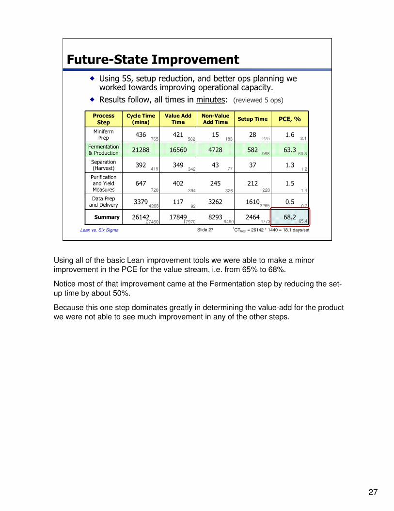
Future-State Improvement
� Using 5S, setup reduction, and better ops planning we worked towards improving operational capacity.
� Results follow, all times in minutes: (reviewed 5 ops)
0.5161032621173379Data Prep
and Delivery
63.358247281656021288Fermentation & Production
68.2246482931784926142Summary
1.5212245402647Purification and Yield Measures
1.33743349392Separation(Harvest)
1.62815421436Miniferm Prep
PCE, %Setup TimeNon-ValueAdd Time
Value AddTime
Cycle Time(mins)
Process Step
4773
765
419
720
4268
275
968
228
3265
582 183
342
394
92
77
326
27460 17970 9490
2.1
60.3
1.2
1.4
0.3
65.4
*CTtotal = 26142 * 1440 = 18.1 days/set
Using all of the basic Lean improvement tools we were able to make a minor improvement in the PCE for the value stream, i.e. from 65% to 68%.
Notice most of that improvement came at the Fermentation step by reducing the set-up time by about 50%.
Because this one step dominates greatly in determining the value-add for the product we were not able to see much improvement in any of the other steps.
28
Lean vs. Six Sigma Slide 28
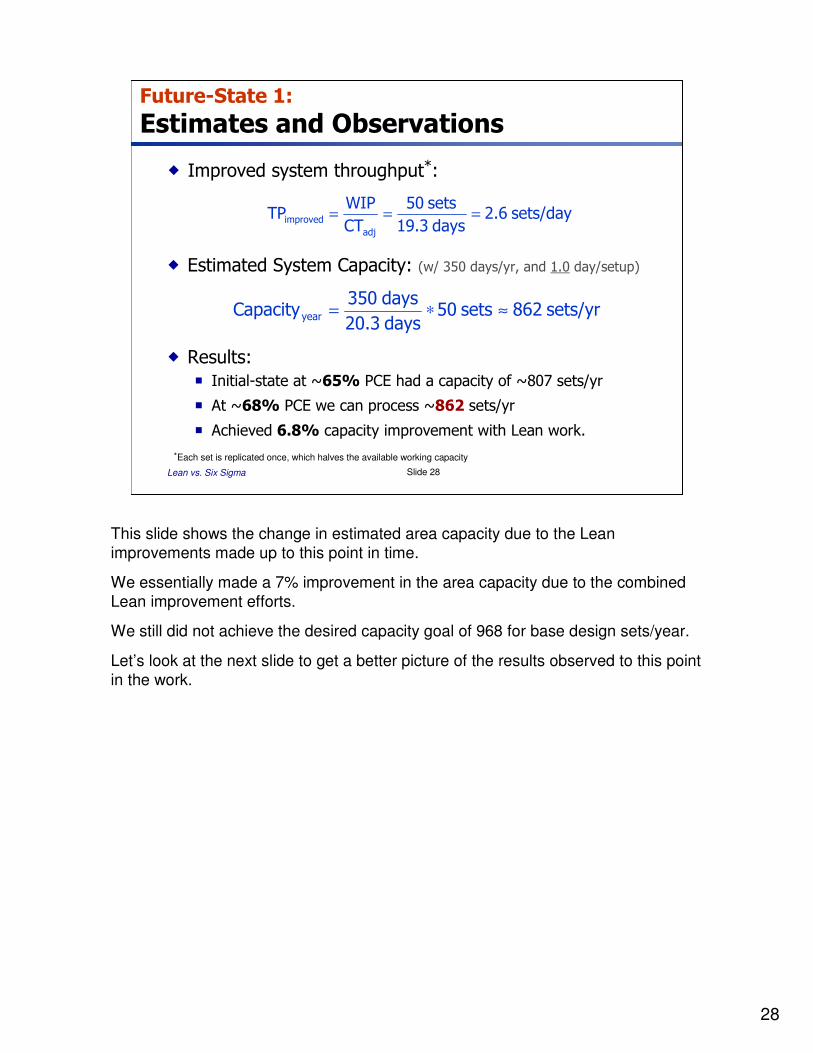
Future-State 1:
Estimates and Observations
� Improved system throughput*:
sets/day 2.6days 19.3
sets 50
CT
WIPTP
adj
improved ===
*Each set is replicated once, which halves the available working capacity
� Estimated System Capacity: (w/ 350 days/yr, and 1.0 day/setup)
sets/yr 862sets 50days 20.3
days 350apacityC year ≈∗=
� Results:
� Initial-state at ~65% PCE had a capacity of ~807 sets/yr
� At ~68% PCE we can process ~862 sets/yr
� Achieved 6.8% capacity improvement with Lean work.
This slide shows the change in estimated area capacity due to the Lean improvements made up to this point in time.
We essentially made a 7% improvement in the area capacity due to the combined Lean improvement efforts.
We still did not achieve the desired capacity goal of 968 for base design sets/year.
Let’s look at the next slide to get a better picture of the results observed to this point in the work.
29
Lean vs. Six Sigma Slide 29
750
800
850
950
1000
900
Capacity, sets/yr
Present
State
Capacity
Goal
Future
State 1
Future
State 2
Ideal
State
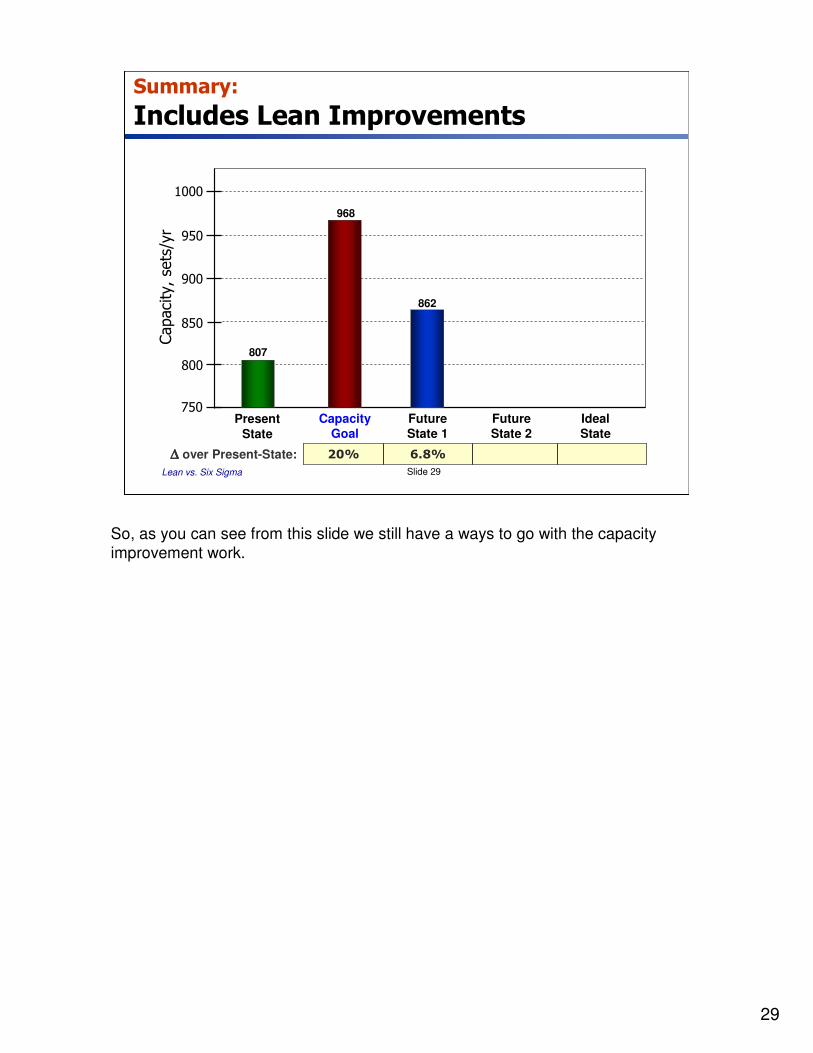
Summary:
Includes Lean Improvements
807
968
862
∆∆∆∆ over Present-State: 6.8%20%
So, as you can see from this slide we still have a ways to go with the capacity improvement work.
30
Lean vs. Six Sigma Slide 30
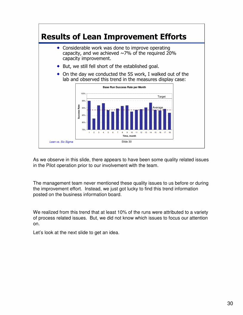
Results of Lean Improvement Efforts
� Considerable work was done to improve operating capacity, and we achieved ~7% of the required 20% capacity improvement.
� But, we still fell short of the established goal.
� On the day we conducted the 5S work, I walked out of the lab and observed this trend in the measures display case:
Base Run Success Rate per Month
75%
80%
85%
90%
95%
100%
1 2 3 4 5 6 7 8 9 10 11 12 13 14 15 16 17 18
Time, month
Su
cc
es
s R
ate
Target
Average
As we observe in this slide, there appears to have been some quality related issues in the Pilot operation prior to our involvement with the team.
The management team never mentioned these quality issues to us before or during the improvement effort. Instead, we just got lucky to find this trend information posted on the business information board.
We realized from this trend that at least 10% of the runs were attributed to a variety of process related issues. But, we did not know which issues to focus our attention on.
Let’s look at the next slide to get an idea.
31
Lean vs. Six Sigma Slide 31
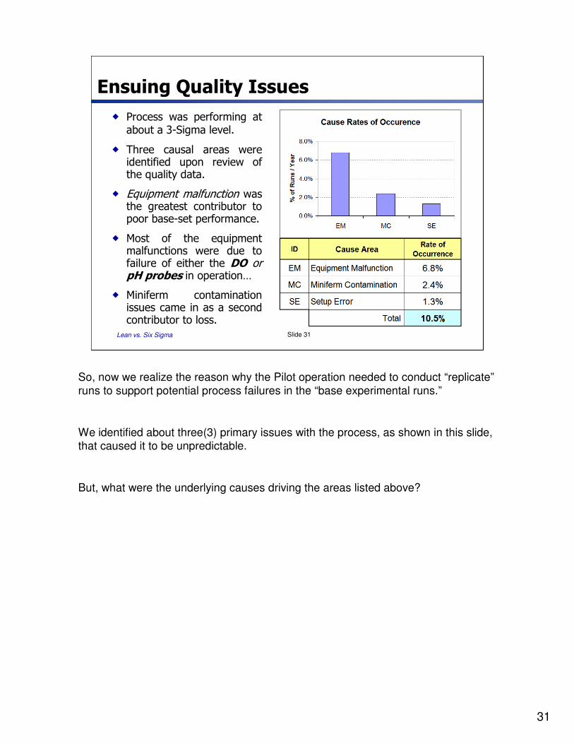
Ensuing Quality Issues
� Process was performing at about a 3-Sigma level.
� Three causal areas were identified upon review of the quality data.
� Equipment malfunction was the greatest contributor to poor base-set performance.
� Most of the equipment malfunctions were due to failure of either the DO or pH probes in operation…
� Miniferm contamination issues came in as a second contributor to loss.
So, now we realize the reason why the Pilot operation needed to conduct “replicate”runs to support potential process failures in the “base experimental runs.”
We identified about three(3) primary issues with the process, as shown in this slide, that caused it to be unpredictable.
But, what were the underlying causes driving the areas listed above?
32
Lean vs. Six Sigma Slide 32
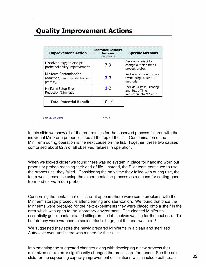
Quality Improvement Actions
Include Mistake Proofing and Setup-Time Reduction into M-Setup
1-2Miniferm Setup Error Reduction/Elimination
10-14Total Potential Benefit:
Recharacterize Autoclave Cycle using SS DMAICmethods
2-3Miniferm Contamination reduction, (improve sterilization process)
Develop a reliability change out plan for all process probes
7-9Dissolved oxygen and pH probe reliability improvement
Specific MethodsEstimated Capacity
Increase (Sets/Month)
Improvement Action
In this slide we show all of the root-causes for the observed process failures with the individual MiniFerm probes located at the top of the list. Contamination of the MiniFerm during operation is the next cause on the list. Together, these two causes comprised about 82% of all observed failures in operation.
When we looked closer we found there was no system in place for handling worn out probes or probes reaching their end-of-life. Instead, the Pilot team continued to use the probes until they failed. Considering the only time they failed was during use, the team was in essence using the experimentation process as a means for sorting good from bad (or worn out) probes!
Concerning the contamination issue--it appears there were some problems with the Miniferm storage procedure after cleaning and sterilization. We found that once the Miniferms were prepared for the next experiments they were placed onto a shelf in the area which was open to the laboratory environment. The cleaned Miniferms essentially got re-contaminated sitting on the lab shelves waiting for the next use. To be fair they were wrapped in sealed plastic bags, but the seal was poor!
We suggested they store the newly prepared Miniferms in a clean and sterilized Autoclave oven until there was a need for their use.
Implementing the suggested changes along with developing a new process that minimized set-up error significantly changed the process performance. See the next slide for the supporting capacity improvement calculations which include both Lean
33
Lean vs. Six Sigma Slide 33
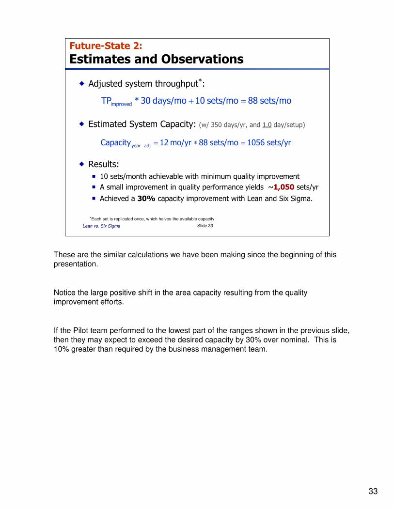
Future-State 2:
Estimates and Observations
� Adjusted system throughput*:
sets/mo 88 sets/mo 10days/mo 30*TPimproved =+
*Each set is replicated once, which halves the available capacity
� Estimated System Capacity: (w/ 350 days/yr, and 1.0 day/setup)
sets/yr 1056sets/mo 88 mo/yr 12apacityC adjyear =∗=−
� Results:
� 10 sets/month achievable with minimum quality improvement
� A small improvement in quality performance yields ~1,050 sets/yr
� Achieved a 30% capacity improvement with Lean and Six Sigma.
These are the similar calculations we have been making since the beginning of this presentation.
Notice the large positive shift in the area capacity resulting from the quality improvement efforts.
If the Pilot team performed to the lowest part of the ranges shown in the previous slide, then they may expect to exceed the desired capacity by 30% over nominal. This is 10% greater than required by the business management team.
34
Lean vs. Six Sigma Slide 34
750
800
850
950
1000
900
Capacity, sets/yr
Present
State
Capacity
Goal
Future
State 1
Future
State 2
Ideal
State
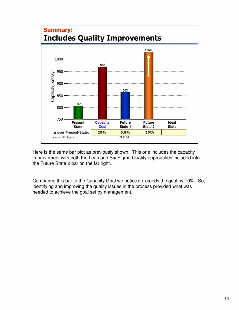
Summary:
Includes Quality Improvements
807
968
862
∆∆∆∆ over Present-State: 30%6.8%20%
1050
Here is the same bar plot as previously shown. This one includes the capacity improvement with both the Lean and Six Sigma Quality approaches included into the Future State 2 bar on the far right.
Comparing this bar to the Capacity Goal we notice it exceeds the goal by 10%. So, identifying and improving the quality issues in the process provided what was needed to achieve the goal set by management.
35
Lean vs. Six Sigma Slide 35
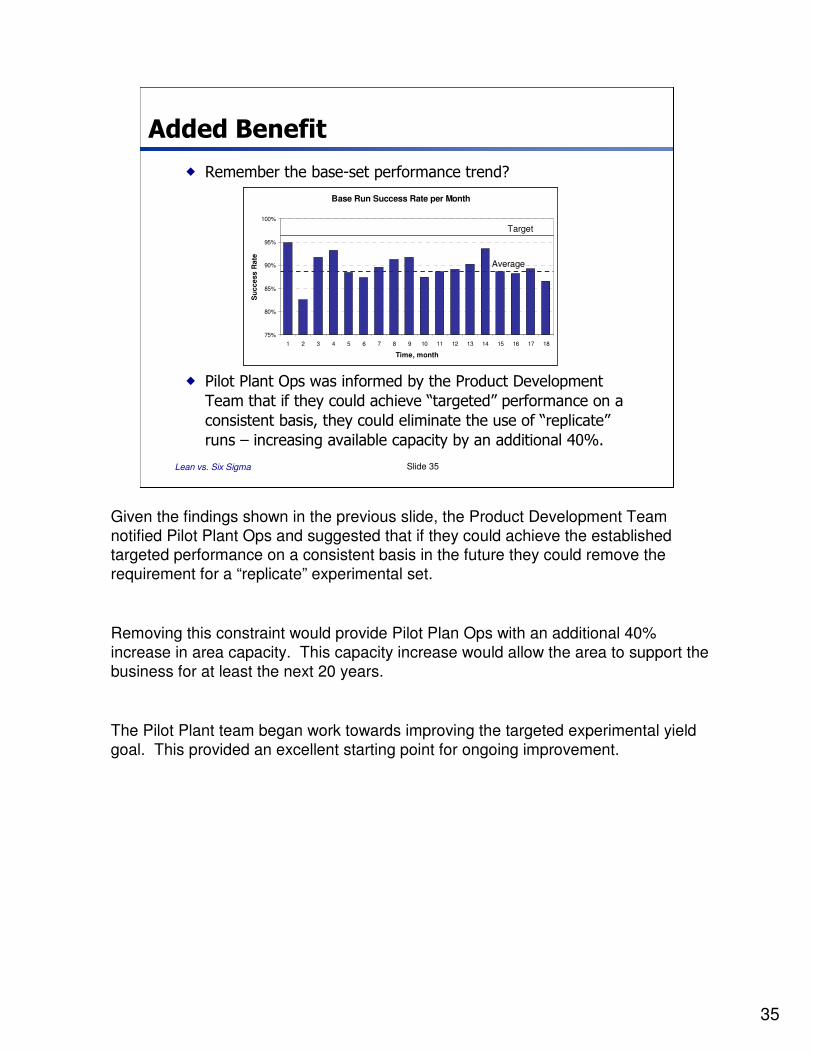
Added Benefit
� Remember the base-set performance trend?
Base Run Success Rate per Month
75%
80%
85%
90%
95%
100%
1 2 3 4 5 6 7 8 9 10 11 12 13 14 15 16 17 18
Time, month
Su
cc
ess
Ra
te
Target
Average
Base Run Success Rate per Month
75%
80%
85%
90%
95%
100%
1 2 3 4 5 6 7 8 9 10 11 12 13 14 15 16 17 18
Time, month
Su
cc
ess
Ra
te
Target
Average
� Pilot Plant Ops was informed by the Product Development
Team that if they could achieve “targeted” performance on a
consistent basis, they could eliminate the use of “replicate”
runs – increasing available capacity by an additional 40%.
Given the findings shown in the previous slide, the Product Development Team notified Pilot Plant Ops and suggested that if they could achieve the established targeted performance on a consistent basis in the future they could remove the requirement for a “replicate” experimental set.
Removing this constraint would provide Pilot Plan Ops with an additional 40% increase in area capacity. This capacity increase would allow the area to support the business for at least the next 20 years.
The Pilot Plant team began work towards improving the targeted experimental yield goal. This provided an excellent starting point for ongoing improvement.
36
Lean vs. Six Sigma Slide 36
750
800
850
950
1000
900
Capacity, sets/yr
Present
State
Capacity
Goal
Future
State 1
Future
State 2
Ideal
State
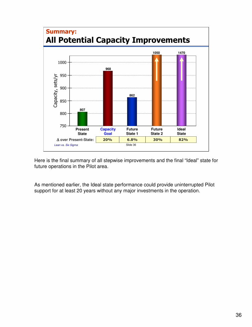
Summary:
All Potential Capacity Improvements
807
968
862
∆∆∆∆ over Present-State: 82%30%6.8%20%
1050 1470
Here is the final summary of all stepwise improvements and the final “Ideal” state for future operations in the Pilot area.
As mentioned earlier, the Ideal state performance could provide uninterrupted Pilot support for at least 20 years without any major investments in the operation.
37
Lean vs. Six Sigma Slide 37
So Which is Better?
� Lean is a management system that can be used to improve the flow of operations in any business.
� Six Sigma is an improvement methodology used to identify and reduce process variation. (a root-muda)
� Six Sigma is also a design methodology used to develop new products and services with low variation.
� Together both methods supply business with the tools needed to improve performance and provide high quality products and services to their customers.

38
InformationalBrief
2012, All Rights Reserved
AppendixAppendix
39
Lean vs. Six Sigma Slide 39
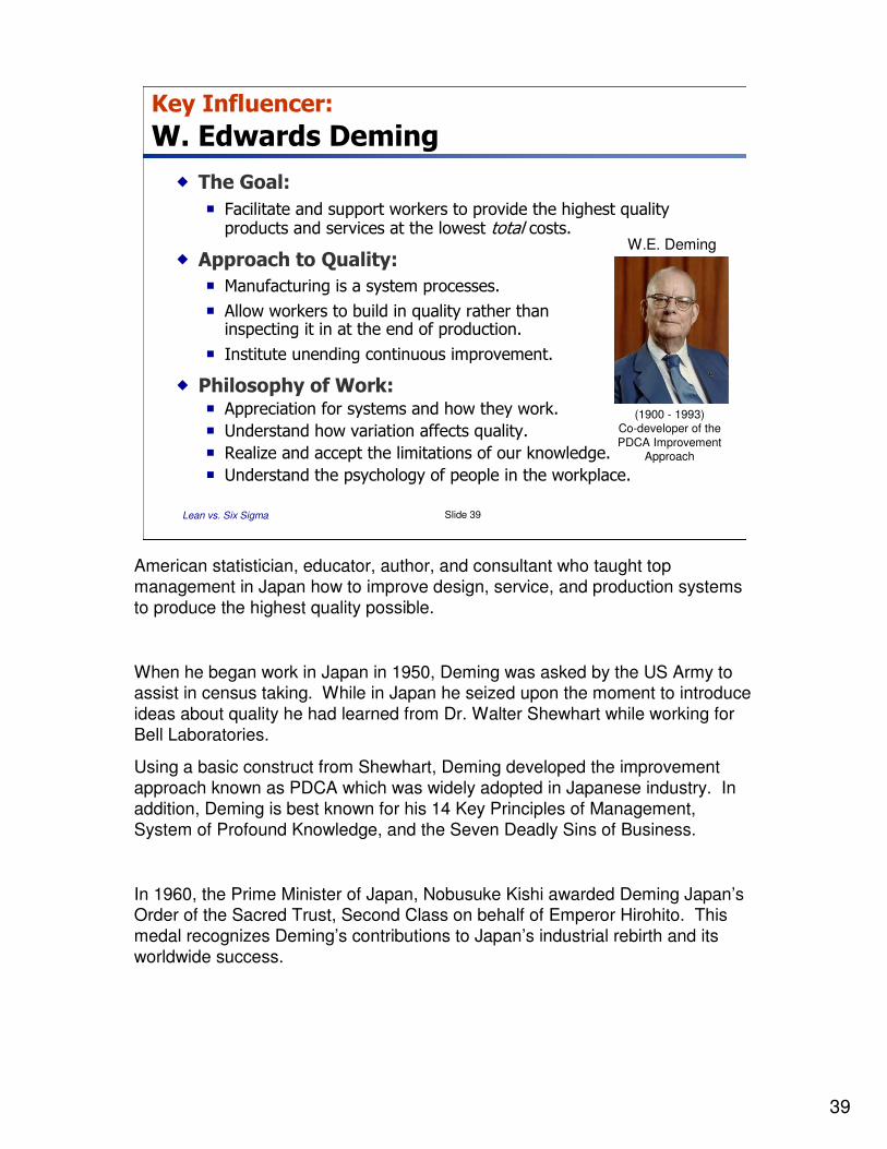
Key Influencer:
W. Edwards Deming
� The Goal:
� Facilitate and support workers to provide the highest quality products and services at the lowest total costs.
� Approach to Quality:
� Manufacturing is a system processes.
� Allow workers to build in quality rather thaninspecting it in at the end of production.
� Institute unending continuous improvement.
� Philosophy of Work:� Appreciation for systems and how they work.
� Understand how variation affects quality.
� Realize and accept the limitations of our knowledge.
� Understand the psychology of people in the workplace.
W.E. Deming
(1900 - 1993)Co-developer of thePDCA Improvement
Approach
American statistician, educator, author, and consultant who taught top management in Japan how to improve design, service, and production systems to produce the highest quality possible.
When he began work in Japan in 1950, Deming was asked by the US Army to assist in census taking. While in Japan he seized upon the moment to introduce ideas about quality he had learned from Dr. Walter Shewhart while working for Bell Laboratories.
Using a basic construct from Shewhart, Deming developed the improvement approach known as PDCA which was widely adopted in Japanese industry. In addition, Deming is best known for his 14 Key Principles of Management, System of Profound Knowledge, and the Seven Deadly Sins of Business.
In 1960, the Prime Minister of Japan, Nobusuke Kishi awarded Deming Japan’s Order of the Sacred Trust, Second Class on behalf of Emperor Hirohito. This medal recognizes Deming’s contributions to Japan’s industrial rebirth and its worldwide success.
40
Lean vs. Six Sigma Slide 40
Key Influencer:
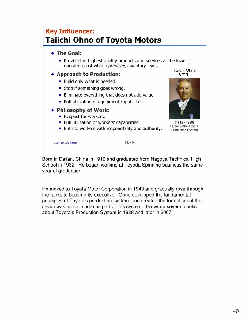
Taiichi Ohno of Toyota Motors
� The Goal:
� Provide the highest quality products and services at the lowest operating cost while optimizing inventory levels.
� Approach to Production:
� Build only what is needed.
� Stop if something goes wrong.
� Eliminate everything that does not add value.
� Full utilization of equipment capabilities.
� Philosophy of Work:� Respect for workers.
� Full utilization of workers' capabilities.
� Entrust workers with responsibility and authority.
Taiichi Ohno大野耐(1912 - 1990)
Father of the Toyota Production System
Born in Dalian, China in 1912 and graduated from Nagoya Technical High School in 1932. He began working at Toyoda Spinning business the same year of graduation.
He moved to Toyota Motor Corporation in 1943 and gradually rose through the ranks to become its executive. Ohno developed the fundamental principles of Toyota’s production system, and created the formalism of the seven wastes (or muda) as part of this system. He wrote several books about Toyota’s Production System in 1988 and later in 2007.
41
Lean vs. Six Sigma Slide 41
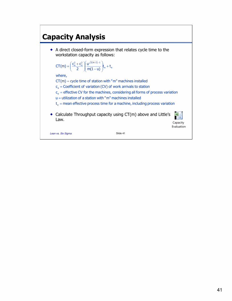
Capacity Analysis
� A direct closed-form expression that relates cycle time to the workstation capacity as follows:
variationprocess including machine, afor time process effective meant
installed machines m"" with station a of nutilizatiou
variationprocess of forms all gconsiderin machines, thefor CV effectivec
station to arrivals work of (CV) variationof tCoefficienc
installed machines m"" with station of time cycle)m(CT
,where
tt)u1(m
u
2
cc)m(CT
e
e
a
ee
1)1m(22e
2a
=
=
=
=
=
+
−
+=
−+
� Calculate Throughput capacity using CT(m) above and Little’s Law.
Capacity
Evaluation
42
Lean vs. Six Sigma Slide 42
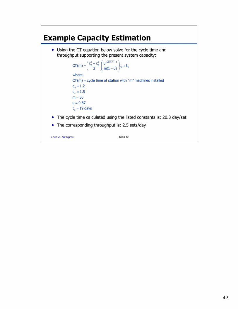
Example Capacity Estimation
� Using the CT equation below solve for the cycle time and throughput supporting the present system capacity:
days 19t
87.0u
50m
5.1c
2.1c
installed machines m"" with station of time cycle)m(CT
,where
tt)u1(m
u
2
cc)m(CT
e
e
a
ee
1)1m(22e
2a
=
=
=
=
=
=
+
−
+=
−+
� The cycle time calculated using the listed constants is: 20.3 day/set
� The corresponding throughput is: 2.5 sets/day
43
Lean vs. Six Sigma Slide 43
Key Influencer:
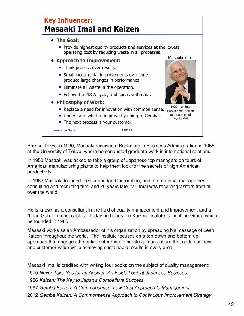
Masaaki Imai and Kaizen
� The Goal:
� Provide highest quality products and services at the lowest operating cost by reducing waste in all processes.
� Approach to Improvement:
� Think process over results.
� Small incremental improvements over time produce large changes in performance.
� Eliminate all waste in the operation.
� Follow the PDCA cycle, and speak with data.
� Philosophy of Work:
� Replace a need for innovation with common sense.
� Understand what to improve by going to Gemba.
� The next process is your customer.
Masaaki Imai
(1930 – to date)
Popularized Kaizenapproach used
at Toyota Motors
Born in Tokyo in 1930, Masaaki received a Bachelors in Business Administration in 1955 at the University of Tokyo, where he conducted graduate work in international relations.
In 1950 Masaaki was asked to take a group of Japanese top managers on tours of American manufacturing plants to help them look for the secrets of high American productivity.
In 1962 Masaaki founded the Cambridge Corporation, and international management consulting and recruiting firm, and 20 years later Mr. Imai was receiving visitors from all over the world
He is known as a consultant in the field of quality management and improvement and a “Lean Guru” in most circles. Today he heads the Kaizen Institute Consulting Group which he founded in 1985.
Masaaki works as an Ambassador of his organization by spreading his message of Lean Kaizen throughout the world. The institute focuses on a top-down and bottom-up approach that engages the entire enterprise to create a Lean culture that adds business and customer value while achieving sustainable results in every area.
Masaaki Imai is credited with writing four books on the subject of quality management:
1975 Never Take Yes for an Answer: An Inside Look at Japanese Business
1986 Kaizen: The Key to Japan’s Competitive Success
1997 Gemba Kaizen: A Commonsense, Low-Cost Approach to Management
2012 Gemba Kaizen: A Commonsense Approach to Continuous Improvement Strategy
44
Lean vs. Six Sigma Slide 44
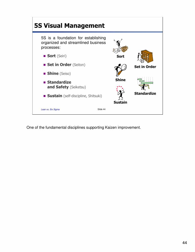
5S Visual Management
Sort
Set in Order
Sustain
Standardize
Shine
5S is a foundation for establishing organized and streamlined business processes:
� Sort (Seiri)
� Set in Order (Seiton)
� Shine (Seiso)
� Standardize and Safety (Seiketsu)
� Sustain (self-discipline, Shitsuki)
One of the fundamental disciplines supporting Kaizen improvement.
45
Lean vs. Six Sigma Slide 45
Goal of all “For Profit” Businesses
� Provide products and services that meet customer needs.
� Improve customer value through the efficient management of business costs.
� Ensure reliable products and services by building quality into all business systems.
� Maintain a competitive edge by continually improving all business processes.