Learning 6D Object Pose Estimationusing 3D Object Coordinates

Eric Brachmann1, Alexander Krull1, Frank Michel1, Stefan Gumhold1, JamieShotton2, and Carsten Rother1

1 TU Dresden, Dresden, Germany2 Microsoft Research, Cambridge, UK

Abstract. This work addresses the problem of estimating the 6D Poseof specific objects from a single RGB-D image. We present a flexible ap-proach that can deal with generic objects, both textured and texture-less.The key new concept is a learned, intermediate representation in form ofa dense 3D object coordinate labelling paired with a dense class labelling.We are able to show that for a common dataset with texture-less objects,where template-based techniques are suitable and state-of-the art, ourapproach is slightly superior in terms of accuracy. We also demonstratethe benefits of our approach, compared to template-based techniques, interms of robustness with respect to varying lighting conditions. Towardsthis end, we contribute a new ground truth dataset with 10k images of20 objects captured each under three different lighting conditions. Wedemonstrate that our approach scales well with the number of objectsand has capabilities to run fast.

1 Introduction

The tasks of object instance detection and pose estimation are well-studied prob-lems in computer vision. In this work we consider a specific scenario where theinput is a single RGB-D image. Given the extra depth channel it becomes feasi-ble to extract the full 6D pose (3D rotation and 3D translation) of rigid objectinstances present in the scene. The ultimate goal is to design a system thatis fast, scalable, robust and highly accurate and works well for generic objects(both textured and texture-less) present in challenging real-world settings, suchas cluttered environments and with variable lighting conditions.

For many years the main focus in the field of detection and 2D/6D poseestimation of rigid objects has been limited to objects with sufficient amountof texture. Based on the pioneering work of [11, 15], practical, robust solutionshave been designed which scale to large number of object instances [18, 20].For textured objects the key to success, for most systems, is the use of a sparserepresentation of local features, either hand crafted, e.g. SIFT features, or trainedfrom data. These systems run typically a two-stage pipeline: a) putative sparsefeature matching, b) geometric verification of the matched features.

Recently, people have started to consider the task of object instance detec-tion for texture-less or texture-poor rigid objects, e.g. [7, 8, 21]. For this partic-ular challenge it has been shown that template-based techniques are superior.

2 authors running

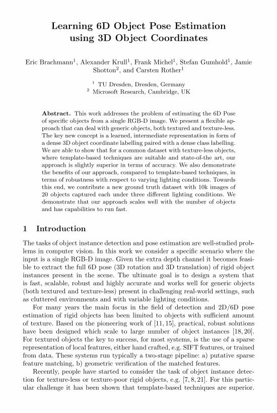
a) b) c) d)

Fig. 1. Overview of our system. Top left: RGB-D Test image (upper-half depth imageand lower-half RGB image). The estimated 6D pose of the query object (camera) isillustrated with a blue bounding box, and the respective ground truth with a greenbounding box. Top right: Visualization of the algorithms search for the optimal pose,where the inlet is a zoom of the centre area. The algorithm optimizes our energyin a RANSAC-like fashion over a large, continuous 6D pose space. The 6D poses,projected to the image plane, which are visited by the algorithm are color coded: redposes are disregarded in a very fast geometry check; blue poses are evaluated using ourenergy function during intermediate, fast sampling; green poses are subject to the mostexpensive energy refinement step. Bottom, from left to right: (a) Probability map forthe query object, (b) predicted 3D object coordinates from a single tree mapped to theRGB cube, (c) corresponding ground truth 3D object coordinates, (d) overlay of the3D model in blue onto the test image (rendered according to the estimated pose)

The main focus of these works has been to show that template-based tech-niques can be made very fast, by using specific encodings [8] or additionally acascaded framework [21]. The typical problems of template-based techniques,such as not being robust to clutter and occlusions as well as changing light-ing conditions, have been partly overcome by carefully hand-crafted templatesand additional discriminative learning. Nevertheless, template-based techniqueshave in our view two fundamental shortcomings. Firstly, they match the com-plete template to a target image, i.e. encode the object in a particular pose withone “global” feature. In contrast to this, sparse feature-based representationsfor textured objects are “local” and hence such systems are more robust withrespect to occlusions. Secondly, it is an open challenge to make template-basedtechniques work for articulated or deformable object instances, as well as objectclasses, due to the growing number of required templates.

title running 3

Our approach is motivated by recent work in the field of articulated humanpose estimation from a pre-segmented RGB-D image [28]. The basic idea in [28] isnot to predict directly the 60-DOF human pose from an image, but to first regressan intermediate so-called object coordinate representation. This means that eachpixel in the image votes for a continuous coordinate on a canonical body in acanonical pose, termed the Vitruvian Manifold. The voting is done by a randomforest and uses a trained assemble of simple, local feature tests. In the next stepa “geometric validation” is performed, by which an energy function is definedthat compares these correspondences with a parametric body model. Finally, thepose parameters are found by energy minimization. Hence, in spirit, this is akinto the two-stage pipeline of traditional, sparse feature-based techniques but nowwith densely learned features. Subsequent work in [24] applied a similar ideato 6D camera pose estimation, showing that a regression forest can accuratelypredict image-to-world correspondences that are then used to drive a camerapose estimaten. They showed results that were considerably more accurate thana sparse feature-based baseline.

Our system is based on these ideas presented in [28, 24] and applies themto the task of estimating the 6D pose of specific objects. An overview of oursystem is presented in Fig. 1. However, we cannot apply [28, 24] directly since weadditional need an object segmentation mask. Note that the method in [28] canrely on a pre-segmented human shape, and [24] does not require segmentation.To achieve this we jointly predict a dense 3D object coordinate labelling anda dense class labelling. Another major difference to [24] is a clever samplingscheme to avoid unnecessary generation of false hypothesis in the RANSAC-based optimization.

To summarize, the main contribution of our work is a new approachthat has the benefits of local feature-based object detection techniques and stillachieves results that are even slightly superior, in terms of accuracy, to template-based techniques for texture-less object detection. This gives us many conceptualand practical advantages. Firstly, one does not have to train a separate systemfor textured and texture-less objects. Secondly, one can use the same systemfor rigid and non-rigid objects, such as laptops, scissors, and objects in differentstates, e.g. a pot with and without lid. Thirdly, by using local features we gainrobustness with respect to occlusions. Fourthly, by applying a rigorous featurelearning framework we are robust to changes in lighting conditions. Fig. 2 showsthe benefits of our system. The main technical contribution of our work is theuse of a new representation in form of a joint dense 3D object coordinate andobject class labelling. An additional minor contribution is a new dataset of 10kimages of 20 objects captured each under three different lighting conditions andlabelled with accurate 6D pose, which will be made publicly available.

2 Related Work

There is a vast literature in the area of pose estimation and object detection,including instance and category recognition, rigid and articulated objects, and

4 authors running

a) b)

c)

d)

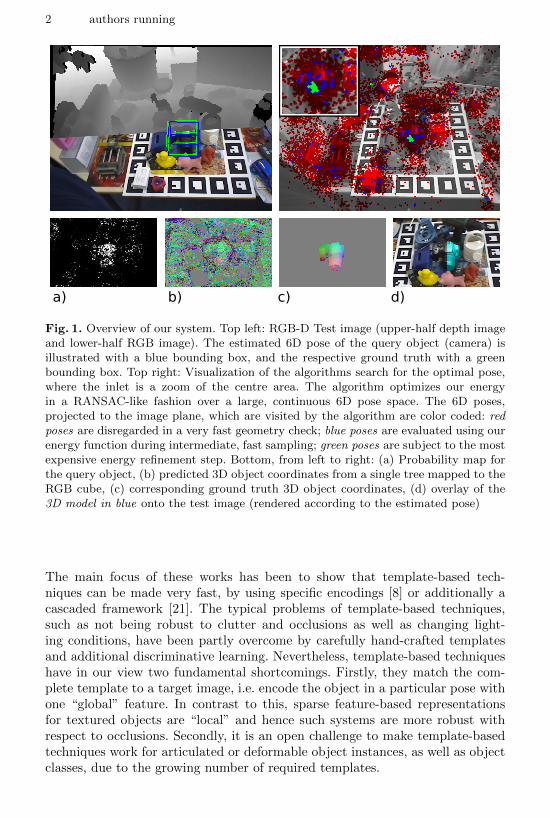
Fig. 2. Our method is able to find the correct pose, where a template-based methodfails. (a) Test image showing a situation with strong occlusion. The pose estimate byour approach is shown in blue. The pose estimated by our reimplementation of themethod by Hinterstoisser et al.from [8] is shown in red. (b) The coordinate predictionsfor a from one tree mapped to the RGB-cube and multiplied with pc,i. (c) Ground truthobject coordinates for a mapped to the RGB-cube. (d) Test image showing extremelight conditions, different from the training set. Estimated poses are displayed as in a

coarse (quantized) and accurate (6D) poses. In the brief review below, we focuson techniques that specifically address the detection of instances of rigid objectsin cluttered scenes and simultaneously infer their 6D pose. Some of the workwas already mentioned above.

Template-based approaches. Perhaps the most traditional approach to ob-ject detection is to use templates, e.g.[11, 26, 7, 8]. This means a rigid templateis scanned across the image, and a distance measure is computed to find thebest match. As the state of the art in template-based approaches, [8] uses syn-thetic renderings of a 3D object model to generate a large number of templatescovering the full view hemisphere. They employ an edge-based distance metricwhich works well for textureless objects, and refine their pose estimates usingICP to achieve an accurate 6D pose. Such template-based approaches can workaccurately and quickly in practice. The limitations of template-based approacheswere discussed above.

Sparse feature-based approaches. A popular alternative to templates aresparse feature-based approaches. These extract points of interest (often scale-invariant) from the image, describe these with local descriptors (often affineand illumination invariant), and match to a database. For example, Lowe [15]used SIFT descriptors and clustered images from similar viewpoints into a sin-gle model. Another great example of a recent, fast and scalable system is [16].Sparse techniques have been shown to scale well to matching across vast vocab-ularies [18, 20]. More recently a trend has been to learn interest points [22, 10],descriptors [30], and matching [14, 19, 1]. Despite their popularity, a major limi-tation of sparse approaches for real applications is that they require sufficientlytextured objects. Our approach instead can be applied densely at every imagepixel regardless of texture, and can learn what are the most appropriate imagefeatures to exploit. Note that there is also large literature on contour and shapematching, which can deal with texture-less objects, e.g. [29], which is, however,conceptually different to our work.

title running 5

Dense approaches. An alternative to templates and sparse approaches aredense approaches. In these, every pixel produces some prediction about the de-sired output. In the generalized Hough voting scheme, all pixels cast a vote insome quantized prediction space (e.g.2D object center and scale), and the cellwith the most votes is taken as the winner. In [27, 5], Hough voting was usedfor object detection, and was shown able to predict coarse object poses. In ourwork we borrow an idea from Gall et al.[5] to jointly train an objective over bothHough votes and object segmentations. However, in contrast to [5] we found asimple joint distribution over the outputs (in our case 3D object coordinatesand object class labeling) to perform better than the variants suggested in [5].Drost et al.[4] also take a voting approach, and use oriented point pair featuresto reduce the search space. To obtain a full 6D pose, one could imagine a variantof [5] that has every pixel vote directly for a global quantized 6D pose. How-ever, the high dimensionality of the search space (and thus the necessary highdegree of quantization) is likely to result in a poor estimate of the pose. In ourapproach, each pixel instead makes a 3D continuous prediction about only itslocal correspondence to a 3D model. This massively reduces the search space,and, for learning a discriminative prediction, allows a much reduced training setsince each point on the surface of the object does not need to be seen from everypossible angle. We show how these 3D object correspondences can efficientlydrive a subsequent model fitting stage to achieve a highly accurate 6D objectpose.

Finally, there are approaches for object class detection that use a similaridea as our 3D object coordinate representation. One of the first systems isthe 3D LayoutCRF [9] which considers the task of predicting a dense part-labelling, covering the 3D rigid object, using a decision forest, though they didnot attempt to fit a 3D model to those labels. After that the Vitruvian Manifold[28] was introduced for human pose estimation, and recently the scene coordinateregression forests was introduced for camera re-localization in RGB-D images[24]. Both works were discussed in detail above.

3 Method

We first describe our decision forest, that jointly predicts both 3D object co-ordinates and object instance probabilities. Then we will discuss our energyfunction which is based on forest output. Finally, we will address our RANSACbased optimization scheme.

3.1 Random forest

We use a single decision forest to classify pixels from an RGB-D image. A decisionforest is a set T of decision trees T j . Pixels of an image are classified by eachtree T j and end up in one of the tree’s leafs lj . Our forest is trained in a waythat allows us to gain information about which object ci the pixel i might belongto, as well as what might be its position on this object. We will denote a pixels

6 authors running

position on the object by yi and refer to it as the pixels object coordinate. Eachleaf lj stores a distribution over possible object affiliations p(c|lj), as well asa set of object coordinates yc(l

j) for each possible object affiliation c. yc(lj)

will be referred to as coordinate prediction. In the following we only discuss theinteresting design decisions which are specific to our problem and refer the readerto the supplementary material for a detailed description.

Design and Training of the Forest We build the decision trees using astandard randomized training procedure [2]. We quantized the continuous dis-tributions p(yi|ci) into 5×5×5 = 125 discrete bins. We use an additional bin fora background class. The quantization allows us to use the standard informationgain classification objective during training, which has the ability to cope betterwith the often heavily multi-model distributions p(yi|ci) than a regression objec-tive [6]. As a node split objective that deals with both our discrete distributions,p(ci|lji ) and p(yi|ci, lji ), we use the information gain over the joint distribution.This has potentially 125|C|+ 1 labels, for |C| object instances and background,though many bins are empty and the histograms can be stored sparsely for speed.We found the suggestion in [5] to mix two separate information gain criteria tobe inferior on our data.

An important question is the choice of features evaluated in the tree splits. Welooked at a large number of features, including normal, color, etc.We found thatthe very simple and fast to compute features from [24] performed well, and thatadding extra types of feature did not appear to give a boost in accuracy (but didslow things down). The intuitive explanation is that the learned combination ofsimple features in the tree is able to create complex features that are specializedfor the task defined by the training data and splitting objective. The features in[24] consider depth or color differences from pixels in the vicinity of pixel i andcapture local patterns of context. The features are depth-adapted to make themlargely depth invariant [23]. Each object is segmented for training. If a featuretest reaches outside the object mask, we have to model some kind of backgroundto calculate feature responses. In our experiments we will use uniform noise or asimulated plane the object sits on. We found this to work well and to generalizewell to new unseen images. Putting objects on a plane allows the forest to learncontextual information.

For training, we use randomly sampled pixels from the segmented objectimages and a set of RGB-D background images. After training the tree structurebased on quantized object coordinates, we push training pixels from all objectsthrough the tree and record all the continuous locations y for each object cat each leaf. We then run mean-shift with a Gaussian kernel and bandwidth2.5cm. We use the top mode as prediction yc(l

j) and store it at the leaf. Wefurthermore store at each leaf the percentage of pixels coming from each objectc to approximate the distribution of object affiliations p(c|lj) at the leaf. We alsostore the percentage of pixels from the background set that arrived at lj , andrefer to it as p(bg|lj).Using the Forest Once training is complete we push all pixels in an RGB-D image through every tree of the forest, thus associating each pixel i with a

title running 7

distribution p(c|lji ) and one prediction yc(lji ) for each tree j and each object c.

Here lji is the leaf outcome of pixel i in tree j. The leaf outcome of all trees for a

pixel i is summarized in the vector li = (l0i , . . . , lji , . . . , l

|T |i ). The leaf outcome of

the image is summarized in L = (l1, . . . , ln). After the pixels have been classifiedwe calculate for the object c we are interested in and for each pixel i in theimage a number pc,i by combining the p(c|lji ) stored at the leafs lji . The numberpc,i can be seen as the approximate probability p(ci|li), that a pixel i belongs

to object c given it ended up in all its leaf nodes li = (l0i , . . . , lji , . . . , l

|T |i ). We

will thus refer to the number pc,i as object probability. We calculate the objectprobability as

pc,i =

∏|T |j=1 p(c|l

ji )∏|T |

j=1 p(bg|lj) +∑

c

∏|T |j=1 p(c|l

ji ). (1)

A detailed deduction for Eq. 1 can be found in the supplementary material.

3.2 Energy Function

Our goal is to estimate the 6 DOF pose Hc for an object c. The pose Hc is definedas the rigid body transformation (3D rotation and 3D translation) that maps apoint from object space into camera space. We formulate the pose estimation asan energy optimization problem. To calculate the energy we compare syntheticimages rendered using Hc with the observed depth values D = (d1, . . . , dn) andthe results of the forest L = (l1, . . . , ln). Our energy function is based on threecomponents:

Ec(Hc) = λdepthEdepthc (Hc) + λcoordEcoord

c (Hc) + λobjEobjc (Hc). (2)

While the component Edepthc (H) punishes deviations between the observed and

ideal rendered depth images, the components Ecoordc (H) and Eobj

c (H) punishdeviations from the predictions of the forest. Fig. 3 visualizes the benefits ofeach component. The parameters λdepth, λcoord and λobj reflect the reliability ofthe different observations. We will now describe the components in detail.The Depth Component is defined as

Edepthc (Hc) =

∑i∈MD

c (Hc)f(di, d

∗i (Hc))

|MDc (Hc)|

, (3)

where MDc (H) is the set of pixels belonging to object c. It is derived from

the the pose Hc by rendering the object into the image. Pixels with no depthobservation di are excluded. The term d∗i (Hc) is the depth at pixel i of ourrecorded 3D model for object c rendered with pose Hc. In order to handleinaccuracies in the 3D model we use a robust error function: f(di, d

∗i (H)) =

min (||x(di)− x(d∗i (H))||, τd) /τd, where x(di) denotes the 3D coordinates in thecamera system derived from the depth di. The denominator in the definitionnormalizes the depth component to make it independent of the object’s distanceto the camera.

8 authors running

depth component coordinate component object component final energy

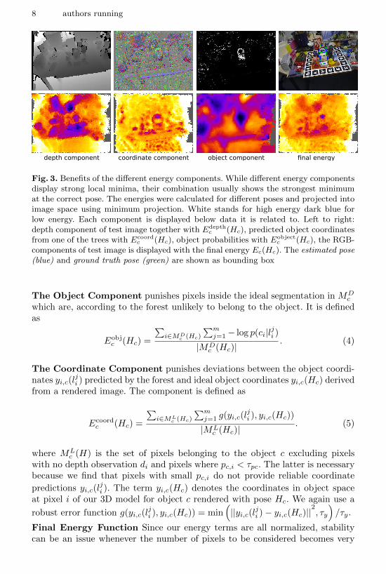
Fig. 3. Benefits of the different energy components. While different energy componentsdisplay strong local minima, their combination usually shows the strongest minimumat the correct pose. The energies were calculated for different poses and projected intoimage space using minimum projection. White stands for high energy dark blue forlow energy. Each component is displayed below data it is related to. Left to right:depth component of test image together with Edepth

c (Hc), predicted object coordinatesfrom one of the trees with Ecoord

c (Hc), object probabilities with Eobjectc (Hc), the RGB-

components of test image is displayed with the final energy Ec(Hc). The estimated pose(blue) and ground truth pose (green) are shown as bounding box

The Object Component punishes pixels inside the ideal segmentation in MDc

which are, according to the forest unlikely to belong to the object. It is definedas

Eobjc (Hc) =

∑i∈MD

c (Hc)

∑mj=1− log p(ci|lji )

|MDc (Hc)|

. (4)

The Coordinate Component punishes deviations between the object coordi-nates yi,c(l

ji ) predicted by the forest and ideal object coordinates yi,c(Hc) derived

from a rendered image. The component is defined as

Ecoordc (Hc) =

∑i∈ML

c (Hc)

∑mj=1 g(yi,c(l

ji ), yi,c(Hc))

|MLc (Hc)|

. (5)

where MLc (H) is the set of pixels belonging to the object c excluding pixels

with no depth observation di and pixels where pc,i < τpc. The latter is necessarybecause we find that pixels with small pc,i do not provide reliable coordinate

predictions yi,c(lji ). The term yi,c(Hc) denotes the coordinates in object space

at pixel i of our 3D model for object c rendered with pose Hc. We again use a

robust error function g(yi,c(lji ), yi,c(Hc)) = min

(||yi,c(lji )− yi,c(Hc)||

2, τy

)/τy.

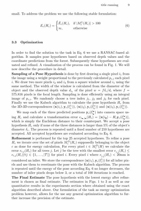
Final Energy Function Since our energy terms are all normalized, stabilitycan be an issue whenever the number of pixels to be considered becomes very

title running 9

small. To address the problem we use the following stable formulation:

Ec(Hc) =

{Ec(Hc), if |ML

c (Hc)| > 100

∞, otherwise(6)

3.3 Optimization

In order to find the solution to the task in Eq. 6 we use a RANSAC-based al-gorithm. It samples pose hypotheses based on observed depth values and thecoordinate predictions from the forest. Subsequently these hypotheses are eval-uated and refined. A visualization of the process can be found in Fig. 1. We willnow describe the procedure in detail.

Sampling of a Pose Hypothesis is done by first drawing a single pixel i1 fromthe image using a weight proportional to the previously calculated pc,i each pixeli. We draw two more pixels i2 and i3 from a square window around i1 using thesame method. The width of the window is calculated from the diameter of theobject and the observed depth value di1 of the pixel w = fδc/di where f =575.816 pixels is the focal length. Sampling is done efficiently using an integralimage of pc,i. We randomly choose a tree index j1, j2 and j3 for each pixel.Finally we use the Kabsch algorithm to calculate the pose hypothesis Hc fromthe 3D-3D-correspondences (x(i1),yc(l

j1i1

)), (x(i2),yc(lj2i2

)) and (x(i3),yc(lj3i3

)).

We map each of the three predicted positions yc(lj•i•

) into camera space us-

ing Hc and calculate a transformation error ei•,j•(Hc) = ||x(i•) − Hcyc(lj•i•

)||,which is simply the Euclidean distance to their counterpart. We accept a posehypothesis Hc only if none of the three distances is larger than 5% of the object’sdiameter δc. The process is repeated until a fixed number of 210 hypotheses areaccepted. All accepted hypotheses are evaluated according to Eq. 6.

Refinement is performed for the top 25 accepted hypotheses. To refine a poseHc we iterate over the set of pixels MD

c (Hc) supposedly belonging to the objectc as done for energy calculation. For every pixel i ∈ MD

c (H) we calculate theerror ei,j(Hc) for all trees j. Let j be the tree with the smallest error ei,j(Hc) ≤ei,j(Hc)|∀j ∈ {1, . . . , |T |} for pixel i. Every pixel i where ei,j(Hc) < 20mm is

considered an inlier. We store the correspondence (x(i1),yc(lji )) for all inlier pix-

els and use them to reestimate the pose with the Kabsch algorithm. The processis repeated until the energy of the pose according Eq. 6 no longer decreases, thenumber of inlier pixels drops below 3, or a total of 100 iterations is reached.

The Final Estimate The pose hypothesis with the lowest energy after refine-ment is chosen as final estimate. The estimates in Figs. 1 to 3 as well as ourquantitative results in the experiments section where obtained using the exactalgorithm described above. Our formulation of the task as energy optimizationproblem however, allows for the use any general optimization algorithm to fur-ther increase the precision of the estimate.

10 authors running

4 Experiments

Several object instance detection datasets have been published in the past [21,3], many of which deal with 2D poses only. Lai et al.[13] published a largeRGB-D dataset of 300 objects that provides ground truth poses in the form ofapproximate rotation angles. Unfortunately, such annotations are to coarse forthe accurate pose estimation task we try to solve. We evaluated our approachon the recently introduced Hinterstoisser et al.[8] dataset and our own dataset.The Hinterstoisser dataset provides synthetic training and real test data. Ourdataset provides real training and real test data with realistic noise patterns andchallenging lighting conditions. On both datasets we compare to the template-based method of [8]. We also tested the scalability of our method and commenton running times. In the supplementary material we provide additional experi-mental results for an occlusion dataset, for a detection task, and regarding thecontribution of our individual energy terms. We train our decision forest withthe following parameters. At each node we sample 500 color features and depthfeatures. In each iteration we choose 1000 random pixels per training image,collect them in the current leafs and stop splitting if less than 50 pixels arrive.The tree depth is not restricted. A complete set of parameters can be found inthe supplement.

Dataset of Hinterstoisser et al. Hinterstoisser et al.[8] provide colored 3Dmodels of 13 texture-less objects3 for training, and 1000+ test images of eachobject on a cluttered desk together with ground truth poses. The test imagescover the upper view hemisphere at different scales and a range of ±45◦ in-plane rotation. The goal is to evaluate the accuracy in pose estimation for oneobject per image. It is known which object is present. We follow exactly the testprotocol of [8] by measuring accuracy as the fraction of test images where thepose of the object was estimated correctly. The tight pose tolerance is definedin the supplementary material. In [8] the authors achieve a strong baseline of96.6% correctly estimated poses, on average. We reimplemented their methodand were able to reproduce these numbers. Their pipeline starts with an efficienttemplate matching schema, followed by two outlier removal steps and iterativeclosest point adjustment. The two outlier removal steps are crucial to achievethe reported results. In essence they comprise of two thresholds on the colorand depth difference, respectively, between the current estimate and the testimage. Unfortunately the correct values differ strongly among objects and haveto be set by hand for each object4. We also compare to [21] who optimize theHinterstoisser templates in a discriminative fashion to boost performance andspeed. They also rely on the same two outlier removal checks but learn the objectdependent thresholds discriminatively.

To produce training data for our method we rendered all 13 object modelswith the same viewpoint sampling as in [8], but skipped scale variations because

3 We had to omit 2 objects since proper 3D models were missing.4 We verified this in private communication with the authors. These values are not

given in the article.

title running 11

of our depth-invariant features. Since our features may reach outside the objectsegmentation during training we need a background model to compute sensiblefeature responses. For our color features we use randomly sampled colors from aset of background images. The background set consists of approx. 1500 RGB-Dimages of cluttered office scenes recorded by ourselfs. For our depth features weuse an infinite synthetic ground-plane as background model. In the test scenesall objects stand on a table but embedded in dense clutter. Hence, we regard thesynthetic plane as an acceptable prior. Additionally, we also show results for abackground model of uniform depth noise, and uniform RGB noise. The decisionforest is trained for all 13 objects and a background class, simultaneously. For thebackground class we sample RGB-D patches from our office background set. Toaccount for variance in appearance between purely synthetic training images andreal test images we add Gaussian noise to the response of the color feature[25].After optimizing our energy, we deploy no outlier removal steps, in contrast to[8, 21].

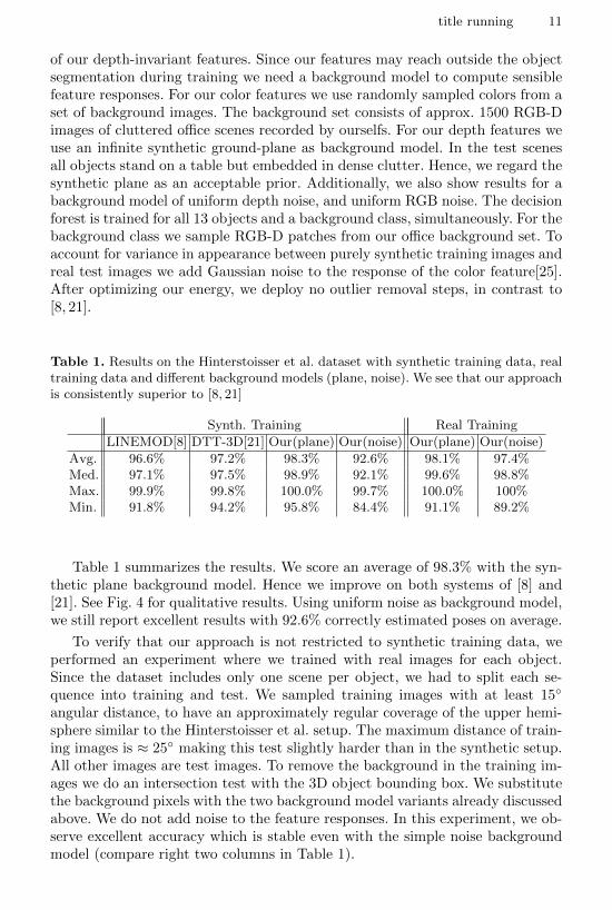
Table 1. Results on the Hinterstoisser et al. dataset with synthetic training data, realtraining data and different background models (plane, noise). We see that our approachis consistently superior to [8, 21]

Synth. Training Real Training

LINEMOD[8] DTT-3D[21] Our(plane) Our(noise) Our(plane) Our(noise)

Avg. 96.6% 97.2% 98.3% 92.6% 98.1% 97.4%Med. 97.1% 97.5% 98.9% 92.1% 99.6% 98.8%Max. 99.9% 99.8% 100.0% 99.7% 100.0% 100%Min. 91.8% 94.2% 95.8% 84.4% 91.1% 89.2%

Table 1 summarizes the results. We score an average of 98.3% with the syn-thetic plane background model. Hence we improve on both systems of [8] and[21]. See Fig. 4 for qualitative results. Using uniform noise as background model,we still report excellent results with 92.6% correctly estimated poses on average.

To verify that our approach is not restricted to synthetic training data, weperformed an experiment where we trained with real images for each object.Since the dataset includes only one scene per object, we had to split each se-quence into training and test. We sampled training images with at least 15◦

angular distance, to have an approximately regular coverage of the upper hemi-sphere similar to the Hinterstoisser et al. setup. The maximum distance of train-ing images is ≈ 25◦ making this test slightly harder than in the synthetic setup.All other images are test images. To remove the background in the training im-ages we do an intersection test with the 3D object bounding box. We substitutethe background pixels with the two background model variants already discussedabove. We do not add noise to the feature responses. In this experiment, we ob-serve excellent accuracy which is stable even with the simple noise backgroundmodel (compare right two columns in Table 1).

12 authors running

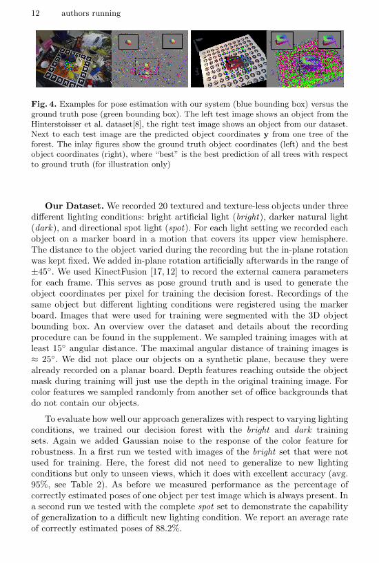
Fig. 4. Examples for pose estimation with our system (blue bounding box) versus theground truth pose (green bounding box). The left test image shows an object from theHinterstoisser et al. dataset[8], the right test image shows an object from our dataset.Next to each test image are the predicted object coordinates y from one tree of theforest. The inlay figures show the ground truth object coordinates (left) and the bestobject coordinates (right), where “best” is the best prediction of all trees with respectto ground truth (for illustration only)

Our Dataset. We recorded 20 textured and texture-less objects under threedifferent lighting conditions: bright artificial light (bright), darker natural light(dark), and directional spot light (spot). For each light setting we recorded eachobject on a marker board in a motion that covers its upper view hemisphere.The distance to the object varied during the recording but the in-plane rotationwas kept fixed. We added in-plane rotation artificially afterwards in the range of±45◦. We used KinectFusion [17, 12] to record the external camera parametersfor each frame. This serves as pose ground truth and is used to generate theobject coordinates per pixel for training the decision forest. Recordings of thesame object but different lighting conditions were registered using the markerboard. Images that were used for training were segmented with the 3D objectbounding box. An overview over the dataset and details about the recordingprocedure can be found in the supplement. We sampled training images with atleast 15◦ angular distance. The maximal angular distance of training images is≈ 25◦. We did not place our objects on a synthetic plane, because they werealready recorded on a planar board. Depth features reaching outside the objectmask during training will just use the depth in the original training image. Forcolor features we sampled randomly from another set of office backgrounds thatdo not contain our objects.

To evaluate how well our approach generalizes with respect to varying lightingconditions, we trained our decision forest with the bright and dark trainingsets. Again we added Gaussian noise to the response of the color feature forrobustness. In a first run we tested with images of the bright set that were notused for training. Here, the forest did not need to generalize to new lightingconditions but only to unseen views, which it does with excellent accuracy (avg.95%, see Table 2). As before we measured performance as the percentage ofcorrectly estimated poses of one object per test image which is always present. Ina second run we tested with the complete spot set to demonstrate the capabilityof generalization to a difficult new lighting condition. We report an average rateof correctly estimated poses of 88.2%.

title running 13

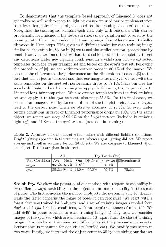
To demonstrate that the template based approach of Linemod[8] does notgeneralize as well with respect to lighting change we used our re-implementationto extract templates for one object based on the training set described above.Note, that the training set contains each view only with one scale. This can beproblematic for Linemod if the test-data shows scale variation not covered by thetraining data. Hence, we render each training image from 2 larger and 3 smallerdistances in 10cm steps. This gives us 6 different scales for each training imagesimilar to the setup in [8]. As in [8] we tuned the outlier removal parameters byhand. However, we found that we had to disable these tests completely to getany detections under new lighting conditions. In a validation run we extractedtemplates from the bright training set and tested on the bright test set. Followingthe procedure of [8], we can estimate correct poses in 80.1% of the images. Weaccount the difference to the performance on the Hinterstoisser dataset[8] to thefact that the object is textured and that our images are noisy. If we test with thesame templates on the spot set, performance drops to 57.1%. Since our tree hasseen both bright and dark in training we apply the following testing procedure toLinemod for a fair comparison. We also extract templates from the dark trainingset and apply it to the spot test set, observing 55.3%. For the final score, weconsider an image solved by Linemod if one of the template sets, dark or bright,lead to the correct pose. Then we observe accuracy of 70.2%. So even undertesting conditions in favor of Linemod performance drops by 10%. On the sameobject, we report accuracy of 96.9% on the bright test set (included in traininglighting), and 91.8% on the spot test set (not seen in training).

Table 2. Accuracy on our dataset when testing with different lighting conditions.Bright lighting appeared in the training set, whereas spot lighting did not. We reportaverage and median accuracy for our 20 objects. We also compare to Linemod [8] onone object. Details are given in the text

All Toy(Battle Cat)

Test Condition Avg. Med. Our [8](dark) [8](bright) [8](combined)

bright 95.6% 97.7% 96.9% - 80.1% -

spot 88.2% 93.0% 91.8% 55.3% 57.1% 70.2%

Scalability. We show the potential of our method with respect to scalability intwo different ways: scalability in the object count, and scalability in the spaceof poses. The first concerns the number of objects the system is able to identify,while the latter concerns the range of poses it can recognize. We start with aforest that was trained for 5 objects, and a set of training images sampled formdark and bright lighting conditions, with an angular distance of min. 45◦. Weadd ±45◦ in-plane rotation to each training image. During test, we considerimages of the spot set which are at maximum 10◦ apart from the closest trainingimage. This results in the same test difficulty as in the previous experiments.Performance is measured for one object (stuffed cat). We modify this setup intwo ways. Firstly, we increased the object count to 30 by combining our dataset

14 authors running

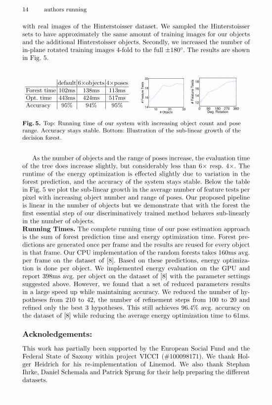
with real images of the Hinterstoisser dataset. We sampled the Hinterstoissersets to have approximately the same amount of training images for our objectsand the additional Hinterstoisser objects. Secondly, we increased the number ofin-plane rotated training images 4-fold to the full ±180◦. The results are shownin Fig. 5.

default 6×objects 4×poses

Forest time 102ms 138ms 113ms

Opt. time 443ms 424ms 517ms

Accuracy 95% 94% 95%10 20 30

14

16

18

20

# Objects

# F

eatu

re T

ests

0 90 180 270 360

12

14

16

18

Deg. Rotation

# F

ea

ture

Te

sts

Fig. 5. Top: Running time of our system with increasing object count and poserange. Accuracy stays stable. Bottom: Illustration of the sub-linear growth of thedecision forest.

As the number of objects and the range of poses increase, the evaluation timeof the tree does increase slightly, but considerably less than 6× resp. 4×. Theruntime of the energy optimization is effected slightly due to variation in theforest prediction, and the accuracy of the system stays stable. Below the tablein Fig. 5 we plot the sub-linear growth in the average number of feature tests perpixel with increasing object number and range of poses. Our proposed pipelineis linear in the number of objects but we demonstrate that with the forest thefirst essential step of our discriminatively trained method behaves sub-linearlyin the number of objects.Running Times. The complete running time of our pose estimation approachis the sum of forest prediction time and energy optimization time. Forest pre-dictions are generated once per frame and the results are reused for every objectin that frame. Our CPU implementation of the random forests takes 160ms avg.per frame on the dataset of [8]. Based on these predictions, energy optimiza-tion is done per object. We implemented energy evaluation on the GPU andreport 398ms avg. per object on the dataset of [8] with the parameter settingssuggested above. However, we found that a set of reduced parameters resultsin a large speed up while maintaining accuracy. We reduced the number of hy-potheses from 210 to 42, the number of refinement steps from 100 to 20 andrefined only the best 3 hypotheses. This still achieves 96.4% avg. accuracy onthe dataset of [8] while reducing the average energy optimization time to 61ms.

Acknoledgements:

This work has partially been supported by the European Social Fund and theFederal State of Saxony within project VICCI (#100098171). We thank Hol-ger Heidrich for his re-implementation of Linemod. We also thank StephanIhrke, Daniel Schemala and Patrick Sprung for their help preparing the differentdatasets.

title running 15

References

1. Bo, L., Ren, X., Fox, D.: Unsupervised feature learning for RGB-D based objectrecognition. In: ISER. (2012)

2. Criminisi, A., Shotton, J.: Decision Forests for Computer Vision and Medical ImageAnalysis. Springer (2013)

3. Damen, D., Bunnun, P., Calway, A., Mayol-Cuevas, W.: Real-time learning anddetection of 3D texture-less objects: A scalable approach. In: BMVC. (2012)

4. Drost, B., Ulrich, M., Navab, N., Ilic, S.: Model globally, match locally: Efficientand robust 3D object recognition. In: CVPR. (2010)

5. Gall, J., Yao, A., Razavi, N., Van Gool, L., Lempitsky, V.: Hough Forests for objectdetection, tracking, and action recognition. IEEE Trans. on PAMI. 33(11) (2011)

6. Girshick, R., Shotton, J., Kohli, P., Criminisi, A., Fitzgibbon, A.: Efficient regres-sion of general-activity human poses from depth images. In: ICCV. (2011)

7. Hinterstoisser, S., Cagniart, C., Ilic, S., Sturm, P., Navab, N., Fua, P., Lepetit, V.:Gradient response maps for real-time detection of texture-less objects. In: IEEETrans. on PAMI. (2012)

8. Hinterstoisser, S., Lepetit, V., Ilic, S., Holzer, S., Bradski, G., Konolige, K., Navab,N.: Model based training, detection and pose estimation of texture-less 3D objectsin heavily cluttered scenes. In: ACCV. (2012)

9. Hoiem, D., Rother, C., Winn, J.: 3D LayoutCRF for multi-view object class recog-nition and segmentation. In: CVPR. (2007)

10. Holzer, S., Shotton, J., Kohli, P.: Learning to efficiently detect repeatable interestpoints in depth data. In: ECCV. (2012)

11. Huttenlocher, D., Klanderman, G., Rucklidge, W.: Comparing images using thehausdorff distance. IEEE Trans. on PAMI. (1993)

12. Izadi, S., Kim, D., Hilliges, O., Molyneaux, D., Newcombe, R., Kohli, P., Shotton,J., Hodges, S., Freeman, D., Davison, A., Fitzgibbon, A.: KinectFusion: real-time3D reconstruction and interaction using a moving depth camera. In: UIST. (2011)

13. Lai, K., Bo, L., Ren, X., Fox, D.: A large-scale hierarchical multi-view rgb-d objectdataset. In: ICRA. IEEE (2011)

14. Lepetit, V., Fua, P.: Keypoint recognition using randomized trees. IEEE Trans. onPAMI. 28(9) (2006)

15. Lowe, D.G.: Local feature view clustering for 3d object recognition. In: CVPR.(2001)

16. Martinez, M., Collet, A., Srinivasa, S.S.: Moped: A scalable and low latency objectrecognition and pose estimation system. In: ICRA. (2010)

17. Newcombe, R., Izadi, S., Hilliges, O., Molyneaux, D., Kim, D., Davison, A., Kohli,P., Shotton, J., Hodges, S., Fitzgibbon, A.: KinectFusion: Real-time dense surfacemapping and tracking. In: ISMAR. (2011)

18. Nister, D., Stewenius, H.: Scalable recognition with a vocabulary tree. In: CVPR.(2006)

19. Ozuysal, M., Calonder, M., Lepetit, V., Fua, P.: Fast keypoint recognition usingrandom ferns. IEEE Trans. on PAMI. (2010)

20. Philbin, J., Chum, O., Isard, M., Sivic, J., Zisserman, A.: Object retrieval withlarge vocabularies and fast spatial matching. In: CVPR. (2007)

21. Rios-Cabrera, R., Tuytelaars, T.: Discriminatively trained templates for 3D objectdetection: A real time scalable approach. In: ICCV. (2013)

22. Rosten, E., Porter, R., Drummond, T.: FASTER and better: A machine learningapproach to corner detection. IEEE Trans. on PAMI. 32 (2010)

16 authors running

23. Shotton, J., Fitzgibbon, A., Cook, M., Sharp, T., Finocchio, M., Moore, R., Kip-man, A., Blake, A.: Real-time human pose recognition in parts from a single depthimage. In: CVPR. (2011)

24. Shotton, J., Glocker, B., Zach, C., Izadi, S., Criminisi, A., Fitzgibbon, A.: Scenecoordinate regression forests for camera relocalization in rgb-d images. In: CVPR.(2013)

25. Shotton, J., Girshick, R.B., Fitzgibbon, A.W., Sharp, T., Cook, M., Finocchio, M.,Moore, R., Kohli, P., Criminisi, A., Kipman, A., Blake, A.: Efficient human poseestimation from single depth images 35(12) (2013)

26. Steger, C.: Similarity measures for occlusion, clutter, and illu-mination invariantobject recognition. In: DAGM-S. (2001)

27. Sun, M., Bradski, G.R., Xu, B.X., Savarese, S.: Depth-encoded hough voting forjoint object detection and shape recovery. In: ECCV. (2010)

28. Taylor, J., Shotton, J., Sharp, T., Fitzgibbon, A.: The Vitruvian Manifold: Infer-ring dense correspondences for one-shot human pose estimation. In: CVPR. (2012)

29. V. Ferrari, F.J., Schmid, C.: From images to shape models for object detection.In: IJCV. (2009)

30. Winder, S., Hua, G., Brown, M.: Picking the best DAISY. In: CVPR. (2009)