Learning Algorithms from Data

by

Wojciech Zaremba

a dissertation submitted in partial fulfillment

of the requirements for the degree of

Doctor of Philosophy

Computer Science

New York University

May, 2016

Rob Fergus

© Wojciech Zaremba

all rights reserved, 2016

Dedication

I dedicate this thesis to the love of my life, Laura Florescu.

iv

Acknowledgments

Pursuing a Ph.D. was one of the best decisions of my life. During

the last several years, I had an opportunity to meet extremely creative and pas-

sionate people, who made my Ph.D. experience profound. Ilya Sutskever is one

of them. He helped me learn what are the right questions to ask and how to

answer them quickly. His invaluable advice was to solve tasks that are on the

brink of insanity and sanity while staying on the sane side. Another person to

whom I owe a lot is Rob Fergus. Rob taught me how to express my thoughts,

how to organize them, and how to present them. Communication is a critical

skill in conveying ideas. There are many others I would like to thank: Geof-

frey Hinton, Yann LeCun, Joan Bruna, Emily Denton, Howard Zhou, the Face-

book AI Research and the Google Brain teams. On the personal side, I am very

grateful to my girlfriend Laura Florescu for her love, support, and being an get-

away for me. Furthermore, several people shaped me as a human being and

gave me a lot of inspiration at the very early stages of my scientific career. My

parents, Irena and Franciszek Zaremba, gave me a lot of love and mental space,

which were critical prerequisites for my development. My brothers Michał and

Maciej Zaremba inspired me by pursuing their own dreams: developing a com-

v

puter game, skydiving, leading a large Scouts organization and many others.

Several early stage teachers ignited my passion and led me to where I am today.

The list includes Jadwiga Grodzicka, Zygmunt Turczyn, Wojciech Zbadyński

and Piotr Pawlikowski. Furthermore, I greatly appreciate the help given by

the Polish Children’s Fund where I met many scientists and talented children,

with emphasis on the scientist Wojciech Augustyniak. Finally, I am thankful to

the members of OpenAI for letting me be a part of this incredible organization.

OpenAI’s environment allows me to redefine the limits of my creativity.

vi

Abstract

Statistical machine learning is concerned with learning models that describe ob-

servations. We train our models from data on tasks like machine translation or

object recognition because we cannot explicitly write down programs to solve

such problems. A statistical model is only useful when it generalizes to unseen

data. Solomonoff114 has proved that one should choose the model that agrees

with the observed data, while preferring the model that can be compressed the

most, because such a choice guarantees the best possible generalization. The

size of the best possible compression of the model is called the Kolmogorov com-

plexity of the model. We define an algorithm as a function with small Kol-

mogorov complexity.

This Ph.D. thesis outlines the problem of learning algorithms from data and

shows several partial solutions to it. Our data model is mainly neural networks

as they have proven to be successful in various domains like object recogni-

tion67,109,122, language modelling90, speech recognition48,39 and others. First, we

examine empirical trainability limits for classical neural networks. Then, we ex-

tend them by providing interfaces, which provide a way to read memory, access

the input, and postpone predictions. The model learns how to use them with re-

inforcement learning techniques like REINFORCE and Q-learning. Next, we ex-

vii

amine whether contemporary algorithms such as convolution layer can be auto-

matically rediscovered. We show that it is possible indeed to learn convolution

as a special case in a broader range of models. Finally, we investigate whether

it is directly possible to enumerate short programs and find a solution to a given

problem. This follows the original line of thought behind the Solomonoff induc-

tion. Our approach is to learn a prior over programs such that we can explore

them efficiently.

viii

Contents

Dedication iv

Acknowledgments v

Abstract vii

1 Introduction 1

1.1 Background - neural networks as function approximators . . . . . 8

1.1.1 Convolutional neural network (CNN) . . . . . . . . . . . . 13

1.1.2 Recurrent neural networks (RNN) . . . . . . . . . . . . . . 14

1.1.3 Long Short-Term Memory (LSTM) . . . . . . . . . . . . . 17

2 Related work 19

3 Limits of trainability for neural networks 24

3.1 Tasks . . . . . . . . . . . . . . . . . . . . . . . . . . . . . . . . . 26

3.2 Curriculum Learning . . . . . . . . . . . . . . . . . . . . . . . . . 29

3.3 Input delivery . . . . . . . . . . . . . . . . . . . . . . . . . . . . . 31

3.4 Experiments . . . . . . . . . . . . . . . . . . . . . . . . . . . . . . 32

3.4.1 Results on the Copy Task . . . . . . . . . . . . . . . . . . 33

ix

3.4.2 Results on the Addition Task . . . . . . . . . . . . . . . . 35

3.4.3 Results on Program Evaluation . . . . . . . . . . . . . . . 35

3.5 Hidden State Allocation Hypothesis . . . . . . . . . . . . . . . . . 37

3.6 Discussion . . . . . . . . . . . . . . . . . . . . . . . . . . . . . . . 40

4 Neural networks with external interfaces 43

4.1 Model . . . . . . . . . . . . . . . . . . . . . . . . . . . . . . . . . 45

4.2 Tasks . . . . . . . . . . . . . . . . . . . . . . . . . . . . . . . . . 48

4.3 Supervised Experiments . . . . . . . . . . . . . . . . . . . . . . . 51

4.4 No Supervision over actions . . . . . . . . . . . . . . . . . . . . . 54

4.4.1 Notation . . . . . . . . . . . . . . . . . . . . . . . . . . . . 55

4.4.2 REINFORCE Algorithm . . . . . . . . . . . . . . . . . . . 57

4.4.3 Q-learning . . . . . . . . . . . . . . . . . . . . . . . . . . . 71

4.4.4 Experiments . . . . . . . . . . . . . . . . . . . . . . . . . 76

4.5 Discussion . . . . . . . . . . . . . . . . . . . . . . . . . . . . . . . 82

5 Learning the convolution algorithm 84

5.1 Spatial Construction . . . . . . . . . . . . . . . . . . . . . . . . . 87

5.1.1 Locality via W . . . . . . . . . . . . . . . . . . . . . . . . 88

5.1.2 Multiresolution Analysis on Graphs . . . . . . . . . . . . . 88

5.1.3 Deep Locally Connected Networks . . . . . . . . . . . . . 89

5.2 Spectral Construction . . . . . . . . . . . . . . . . . . . . . . . . 92

5.2.1 Harmonic Analysis on Weighted Graphs . . . . . . . . . . 92

5.2.2 Extending Convolutions via the Laplacian Spectrum . . . 93

x

5.2.3 Rediscovering standard CNN’s . . . . . . . . . . . . . . . 95

5.2.4 O(1) construction with smooth spectral multipliers . . . . 96

5.2.5 Multigrid . . . . . . . . . . . . . . . . . . . . . . . . . . . 98

5.3 Numerical Experiments . . . . . . . . . . . . . . . . . . . . . . . . 99

5.3.1 Subsampled MNIST . . . . . . . . . . . . . . . . . . . . . 99

5.3.2 MNIST on the sphere . . . . . . . . . . . . . . . . . . . . 102

5.4 Discussion . . . . . . . . . . . . . . . . . . . . . . . . . . . . . . . 106

6 Learning algorithms in attribute grammar 107

6.1 A toy example . . . . . . . . . . . . . . . . . . . . . . . . . . . . 109

6.2 Problem Statement . . . . . . . . . . . . . . . . . . . . . . . . . . 110

6.3 Attribute Grammar . . . . . . . . . . . . . . . . . . . . . . . . . . 111

6.4 Representation of Symbolic Expressions . . . . . . . . . . . . . . 112

6.4.1 Numerical Representation . . . . . . . . . . . . . . . . . . 112

6.4.2 Learned Representation . . . . . . . . . . . . . . . . . . . 113

6.5 Linear Combinations of Trees . . . . . . . . . . . . . . . . . . . . 117

6.6 Search Strategy . . . . . . . . . . . . . . . . . . . . . . . . . . . . 117

6.6.1 Random Strategy . . . . . . . . . . . . . . . . . . . . . . . 119

6.6.2 n-gram . . . . . . . . . . . . . . . . . . . . . . . . . . . . 119

6.6.3 Recursive Neural Network . . . . . . . . . . . . . . . . . . 119

6.7 Experiments . . . . . . . . . . . . . . . . . . . . . . . . . . . . . . 120

6.7.1 Expression Classification using Learned Representation . . 120

6.7.2 Efficient Identity Discovery . . . . . . . . . . . . . . . . . 121

6.7.3 Learnt solutions to (∑

AAT)k . . . . . . . . . . . . . . . 124

xi

6.7.4 Learnt solutions to (RBM-1)k . . . . . . . . . . . . . . . 125

6.7.5 Learnt solutions to (RBM-2)k . . . . . . . . . . . . . . . 127

6.8 Discussion . . . . . . . . . . . . . . . . . . . . . . . . . . . . . . . 130

7 Conclusions 132

7.1 Summary of Contributions . . . . . . . . . . . . . . . . . . . . . . 132

7.2 Future Directions . . . . . . . . . . . . . . . . . . . . . . . . . . . 135

Bibliography 155

xii

1Introduction

Statistical machine learning (ML) is a field concerned with learning patterns

from data without explicitly programming them110. A typical problem in this

field is to learn a parametrized function f . Such a function could map images

to object identities (object recognition67,53,109,122,121), voice recordings to their

transcriptions (speech recognition40,47,94,39), or an English sentence to a foreign

language translation (machine translation118,4,18,81). ML techniques allow us to

train computers to solve such problems without requiring explicit programming

by developers.

In 1964, Solomonoff114 (further formalized by Levine et al.77, and more re-

1

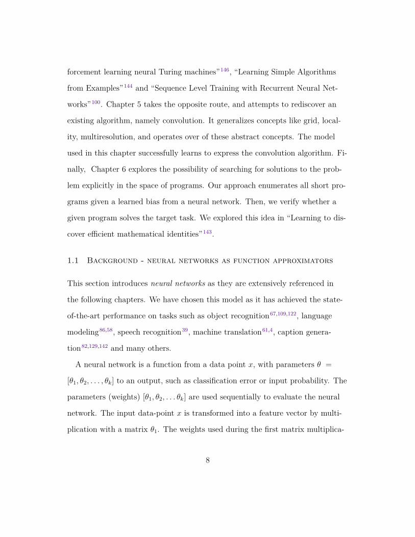
cently by Li and Vitányi78) proved that the function f should be chosen based

on its Kolmogorov complexity, which is the length of the shortest program that

completely specifies it. For instance, the sequence 1, 2, . . . , 10000 has a low

Kolmogorov complexity, because the program that describes it is short:[i for i in range(10000)]

This line of thought reappears under different incarnations across statistical

machine learning. Regularization11, Bayesian inference13, minimum description

length101, VC dimension127 and the Occam’s Razor52,34 principle, all support

choosing the simplest function that fits data well. Many of these concepts re-

gardless of their precision are difficult to be applied. For instance, the VC di-

mension of neural-networks is infinite; therefore, one pays an infinite cost for

using a neural network as the model of data. Moreover, some of the choices in

these techniques are arbitrary. For instance, the prior in case of Bayesian in-

ference, regularization, or Turing machine is an arbitrary choice that has to be

made. The aforementioned concepts can be considered as equivalent130, and in

this thesis we choose to focus on Solomonoff induction and Kolmogorov com-

plexity.

Solomonoff proved that choosing the learning function f based on its Kol-

mogorov complexity guarantees the best possible generalization. The goal of

statistical machine learning is generalization, so machine learning methods should

explore functions according to the length of the program that specifies them.

We define an algorithm to be any function that can be expressed with a short

program. An example of an algorithm is the multi-digit addition process taught

2

in elementary school. This algorithm maps two multi-digit numbers to their

sum. The addition algorithm requires (1) memorizing how to perform single-

digit addition, (2) knowing how to pass the carry, and (3) knowing where to

look up the input data. Since this sequence of steps can be expressed by a short

program, addition is an algorithm. Moreover, classical algorithms such as Di-

jkstra, Bubble sort and the Fourier transform can be expressed with short pro-

grams, and therefore, they are algorithms as well. Even a cooking recipe is an

example of a short program, and hence, an algorithm. An example of a non-

algorithm is a database of users and their passwords. Such a database cannot

be characterized in a simple way without the loss of the user information. An-

other example of a non-short program a procedure that translates Polish words

into English. The English-Polish word correspondence requires storing informa-

tion about every individual word; hence, it is not an algorithm.

Since problems such as machine translation have high Kolmogorov complex-

ities, it is natural to ask why is it important to learn concepts with low Kol-

mogorov complexities. The machine translation function requires storing infor-

mation about the meaning of many words, and, therefore, cannot have small

Kolmogorov complexity. Nonetheless, the optimal model, in regard to Kolmogorov

complexity, should store the smallest number of facts. Such a model should

share the parameters used to represent words such as “teaching” and “teach”.

Similarly, it should understand relationships between affirmative and interrog-

ative sentences and share the parameters used to represent them, while at the

same time being able to translate between all such sentences. The procedure

3

for turning a verb into its progressive tense (to its “+ing” version) is an algo-

rithm, as is the procedure for turning an affirmative sentence into a question. A

highly performing model should internally employ such algorithms while trans-

lating sentences. This is because, the amount of incompressible data that the

model stores determines how well the model generalizes. Given two models with

the same training accuracy, Solomonoff’s114 work shows that the one with the

smaller Kolmogorov complexity generalizes better. Therefore, the optimal model

for machine translation should make use of many such algorithms, so as to mini-

mize the amount of information that needs to be stored.

One can argue that these ideas are partially useful, because one has to choose

Turing machine in order for computation to be valid. In fact, techniques in

Bayesian inference and regularization have the same issues. One has to choose

either a prior, or a regularizer. However, our main interest is in regimes when

the amount of data becomes infinite. We examine whether our statistical mod-

els are able to learn a perfect, deterministic rule which generates data. Finding

such a rule would mean that, through training, neural networks can express dif-

ferent Turing machines with a finite number of symbols versus needing an in-

finite number of symbols to express other concepts. For me, this distinction is

the distinction between understanding and memorizing. Therefore, this is fun-

damental in order to determine intelligence.

This thesis investigates the use of statistical machine learning methods to

learn algorithms from data. Since the best-generalizing models must learn func-

tions with small Kolmogorov complexity, the focus is on developing models that

4

can express algorithms. For example, we examine training a neural network to

learn multi-digit addition based on examples (e.g. input: 12 + 5, target: 17),

where the measure of the success of the addition algorithm is the correctness of

the model’s answers for inputs outside the support of the training distribution.

We do not know the function expressing machine translation because its Kol-

mogorov complexity is not small. Consequently, we are unable to verify whether

a given model makes the best possible use of training data to learn this func-

tion. However, the addition function is known; this allows us to verify whether

the model has indeed learned the desired function, rather than simply memo-

rized millions of examples. Since the Kolmogorov complexity of memorizing ex-

amples is high, a model employing this approach would not generalize to harder

examples.

Intelligence can be perceived as the ability to explain observations using short

programs. For example, Einstein’s general relativity theory has a very low Kol-

mogorov complexity, and his model can explain orbits of Mercury32,33 as accu-

rately as other more complicated models (i.e. models having higher Kolmogorov

complexity). As a result, physicists prefer Einstein’s theory. Similarly, the mod-

els presented here are chosen due to their ability to learn concise description of

data, rather than simply memorize it.

Contemporary machine learning models rely heavily on memorization, which

has high Kolmogorov complexity (Chapter 3). Training on more data gives the

impression of progress because the models perform better on test data. Nonethe-

less, these models are just memorizing data without being able to make sense of

5

it. The growing interest in the Big Data paradigm55,80,141 further encourages

this reliance on memorization. But this reliance on memorization is not new.

Since ancient times, physicists were able to predict the trajectories of stars be-

cause they had large tables of star positions. Their predictions were correct for

examples within the training distribution, but the Kolmogorov complexity of

their model is unnecessarily large. Consequently, their models do not general-

ize well to corner case examples, such as Mercury’s orbit. Space-time warping

significantly influences Mercury due to its proximity to the sun, and, hence,

ancient astronomical tables were inaccurate in fully describing its orbit. The

objective of the models presented in this thesis is to discover fundamental prin-

ciples underlying the phenomenon of interest. By analogy to physicists’ work, it

is preferable for a model to discover the real underlying phenomena such as the

theory of general relativity, rather than to memorize the positions of all stars

at every day of the year. Memorization is a way to compensate for the lack of

understanding. One could argue that this is an old fashion trade-off between

fitting data and model simplicity. However, we consider experiments in the infi-

nite data regime, where over-fitting is not an issue.

The majority of tasks that we consider are from the mathematical realm,

rather than from the perceptive one, as the former have low Kolmogorov com-

plexities. We employ neural networks, because they achieve remarkable per-

formance in various other applications, so there is a hope that neural networks

could learn to encode algorithms as well.

First, we introduce modern neural networks as the primary statistical model

6

used in this thesis. This includes feed-forward networks, convolutional neural

networks, recurrent neural networks, long short term memory units, and the use

of these models to perform sequence-to-sequence mappings (Chapter 1.1). The

chapter presents neural networks as universal approximators, and explains the

relationship between deep architectures and small Kolmogorov complexity. This

chapter is based on a long-standing work in the field, and it briefly refers to our

papers “Recurrent neural network regularization”147 and “An empirical explo-

ration of recurrent network architectures”59. Chapter 2 describes the relation

of the results presented here to those presented in the prior work, and outlines

classical approaches to algorithm learning. Chapter 3 examines the trainability

limits of neural networks. More specifically, given the fact that a neural net-

work can approximate any function (as neural networks are universal approxi-

mators), we investigate how well it can learn to approximate a specific function

in practice. We show that while neural networks can rarely learn the perfect

solution, they can compensate for their lack of true understanding with memo-

rization. Memorization results in remarkable performance on some tasks, even

though the networks could not learn to solve the given task completely. Chap-

ter 3 is based on the paper “Learning to execute”145.

Continuing this line of inquiry, we research how to encourage a neural net-

work to learn a function that generalizes from short sequences correctly to ones

of arbitrary length. Chapter 4 investigates neural networks augmented with ex-

ternal interfaces. These interfaces provide composable building blocks for ex-

pressing algorithms, and the results presented are based on the papers “Rein-

7

forcement learning neural Turing machines”146, “Learning Simple Algorithms

from Examples”144 and “Sequence Level Training with Recurrent Neural Net-

works”100. Chapter 5 takes the opposite route, and attempts to rediscover an

existing algorithm, namely convolution. It generalizes concepts like grid, local-

ity, multiresolution, and operates over of these abstract concepts. The model

used in this chapter successfully learns to express the convolution algorithm. Fi-

nally, Chapter 6 explores the possibility of searching for solutions to the prob-

lem explicitly in the space of programs. Our approach enumerates all short pro-

grams given a learned bias from a neural network. Then, we verify whether a

given program solves the target task. We explored this idea in “Learning to dis-

cover efficient mathematical identities”143.

1.1 Background - neural networks as function approximators

This section introduces neural networks as they are extensively referenced in

the following chapters. We have chosen this model as it has achieved the state-

of-the-art performance on tasks such as object recognition67,109,122, language

modeling86,58, speech recognition39, machine translation61,4, caption genera-

tion82,129,142 and many others.

A neural network is a function from a data point x, with parameters θ =

[θ1, θ2, . . . , θk] to an output, such as classification error or input probability. The

parameters (weights) [θ1, θ2, . . . θk] are used sequentially to evaluate the neural

network. The input data-point x is transformed into a feature vector by multi-

plication with a matrix θ1. The weights used during the first matrix multiplica-

8

Figure 1.1: This diagram presents a graphical representation of a 2-layer neural network. The fig-ure is taken from wikipedia https://en.wikipedia.org/wiki/Artificial_neural_network.

tion are regarded as the parameters of the first layer. Similarly, the n-th matrix

multiplication parameters are called the n-th layer. The matrix multiplication

is followed by an application of the non-linear function σ. The non-linearity is

an element-wise function, and common choice is the sigmoid function: 11+e−x ,

hyperbolic tangent: ex−e−x

ex+e−x , or the rectified linear unit: max(x, 0). The process

of matrix multiplication and composition repeats k times. The output of the

network is the result of this computation, and we refer to it as ϕ(x, θ). Fig. 1.1

presents this concept on a diagram, and the equations below describe it more

formally:

9

Input: x ∈ Rn (1.1)Parameters of the 1-st layer: θ1 ∈ Rn×n1 (1.2)Activations of the 1-st layer: σ(xθ1) ∈ Rn1 (1.3)

Parameters of the 2-nd layer: θ2 ∈ Rn1×n2 (1.4)Activations of the 2-nd layer: σ(σ(xθ1)θ2) ∈ Rn2 . . . (1.5)

Parameters of the (k − 1)-th layer: θk−1 ∈ Rnk−2×nk−1 (1.6)Activations of the (k − 1)-th layer: σ(. . . σ(σ(xθ1)θ2) . . . θk−1) ∈ Rnk−1 (1.7)

Parameters of the k-th layer: θk ∈ Rnk−1×nk (1.8)Output: σ(σ(. . . σ(σ(xθ1)θ2) . . . θk−1)θk) ∈ Rnk (1.9)

Output shortly: ϕ(x, θ) ∈ Rnk (1.10)

Some design choices behind neural networks might look arbitrary. For in-

stance, one can ask why the application of the non-linear function is necessary,

and whether a neural network could attain the same performance without it. In

fact, since the composition of matrix multiplication operations is a linear func-

tion, the neural network would reduce to a single layer transformation. The

properties of the non-linear functions thus extend the expressive power of the

model. The classic example of the need for non-linearity is the task to learn

the exclusive-or (XOR) function (Fig. 1.2). The XOR function cannot be rep-

resented by a linear classifier, because it has a non-linear decision boundary.

The two layer neural network has been proven to be a universal function ap-

proximator24. Consequently, there exist parameters [θ1, θ2], such that any con-

tinuous function g with compact support S can be arbitrarily well approximated

by a neural network. More formally:

10

Figure 1.2: Diagram presents XOR function. Blue points ([0, 0], [1, 1]) have label 1, while redpoints ([0, 1], [1, 0]) have label 0. It is impossible to assign such labels to the points with a linearclassifier, as the decision boundary is not linearly separable.

∀ϵ>0, ∃θ1,θ2∀x∈S, ||σ(xθ1)θ2 − g(x)|| < ϵ. (1.11)

If a two layer neural network can approximate any function, one could ask why

one would need to use more layers. Indeed, there is no expressive power gained

by adding more layers. However, many functions are easier to represent with

several layers. For instance, the parity function requires an exponential num-

ber of parameters to be represented by a two layer neural network, whereas only

a linear number of parameters for a sufficiently deep network137. The theorem

that a two layer neural network is a universal function approximator caused

stagnation in the neural network field for 30 years91. The deep learning paradigm

encourages the use of a larger number of layers, hence use of the word deep.

Deep architectures have proved to be very successful empirically67,39,5,118, be-

cause they force the sharing of the computation, which results in a smaller Kol-

mogorov complexity.

11

The loss function L measures the performance of a model. The goal of learn-

ing is to achieve a low loss over the data distribution:

find θ = argminθ

Ex∼pL(ϕ(x, θ)) (1.12)

Learning is a process of determining model parameters θ = [θ1, . . . , θk] that min-

imize the loss over the data distribution. However, we do not have access to the

entire data distribution. Therefore, learning attempts to achieve low error over

the data distribution by finding parameters that yield low error on the training

data (empirical risk minimization127). There are various ways to learn neural

network parameters based on data, such as the cross-entropy method102, simu-

lated annealing14, genetic programming92 and a few others. However, the single

most popular method of training neural networks is gradient descent. Gradi-

ent descent is a sequential method of updating parameters θ according to their

derivatives with respect to the loss:

θnew := θ − ϵ∂θ

[Ex∼ptrainL(ϕ(x, θ))

](1.13)

The updates of gradient descent are guaranteed to drop the training loss as

long as the step ϵ is sufficiently small, unless θ is a critical point of L(ϕ) (i.e. a

minimum or a saddle point). Conventional training consists of several changes

to the original formulation of gradient descent. These changes include using

only part of the data instead of all of it to determine each parameter update

(stochastic gradient descent28), incorporating momentum, applying batch nor-

12

malization54 etc. Other advances deal with compressing θ by reusing it. For in-

stance, a convolution layer75 uses a banded matrix θi (as convolutional kernels

are locally connected), and θi has many repeated entries due to weight shar-

ing. Such a matrix θi is much smaller in the number of parameters than an ar-

bitrary matrix. We discuss more details of convolutional neural networks in Sec-

tion 1.1.1. Another choice of sharing parameters has to do with processing se-

quences. A recurrent neural network7,10 (RNN) is a neural network that shares

parameters over time. Therefore, every time slice is processed by a network hav-

ing the same parameters. We use RNNs in this thesis extensively, hence Sec-

tion 1.1.2 describes them in details.

1.1.1 Convolutional neural network (CNN)

The convolutional layer is a linear layer with constraints on the weights. It as-

sumes that the input representation has a grid structure and that nearby values

are correlated. A generic linear layer does not make any assumptions on the

relation between consecutive input entries; thus it requires more data in order

to estimate parameters. The most compelling example of an input with grid

structure is an image. The nearby pixels of an image are highly correlated, and

convolution uses the same weights for all locations. Fig. 1.3 outlines the connec-

tivity pattern for the convolutional layer.

The Kolmogorov complexity is well defined not only for datasets, but also for

models. The Kolmogorov complexity of a model is the smallest size of program

that reproduces parameters of the model. Given the same number of activa-

13

Figure 1.3: (Left) Connectivity pattern for fully connected layer. Every input pixel has a separateset of parameters. (Center) Connectivity pattern for a layer with parameter sharing. Pixels invarious locations are treated using the same weights. (Right) Diagram for convolutional neuralnetwork. Pixels in different areas share weights, and weights act locally (locally receptive fields).Figure adapted with permission from Marc’aurelio Ranzato.

tions, fully connected layers are less compressible than convolution layers which

have small number of parameters in the first place. Therefore, Kolmogorov com-

plexity of a convolutional layer is usually smaller than the Kolmogorov complex-

ity of a fully connected layer, and this implies better generalization. Remark:

It’s possible to construct a fully connected network with tiny Kolmogorov com-

plexity. It’s enough to assign a single constant value to all weights. However,

this contrived example is not of our interest, as we consider Kolmogorov com-

plexity of a model after being trained on a distribution coming from natural

data.

1.1.2 Recurrent neural networks (RNN)

The Recurrent Neural Network (RNN) is a variant of the neural network whose

parameters repeat in a manner that allows arbitrary-length sequences to be pro-

cessed using a finite number of parameters. The RNN achieves this by sharing

parameters over time steps, where time is represented by the sequence index.

14

Notation

Let the subscripts denote time-steps and the superscripts denote layers. All our

states are n-dimensional. Let hlt ∈ Rn be a hidden state in layer l in time-step t.

Moreover, let Tn,m : Rn → Rm be an affine transformation (Wx + b for some

W and b). Let ⊙ be element-wise multiplication and h0t be an input vector at

time-step k.

The RNN dynamics consist of parametric, deterministic transitions from pre-

vious to current hidden states:

RNN : hl−1t , hl

t−1 → hlt (1.14)

The classical RNN uses the following transition functions:

hlt = f(Tn,nh

l−1t + Tn,nh

lt−1), where f ∈ sigmoid, hyperbolic tangent (1.15)

One of the main, classical tasks for RNN is language modeling 117,85. A lan-

guage model is a probabilistic model for sequences. It relies on the mathemati-

cal identity

p(x1, x2, . . . , xk) = Πki=1p(xi|xj<i). (1.16)

An RNN is trained by maximizing the probability p(xi|xj<i). Fig. 1.4 presents

three time-steps of an RNN on the task of language modeling for English. Nowa-

days, the application of RNNs has expanded beyond language modeling, and

15

Figure 1.4: Language modelling task. The RNN tries to predict probability of a word given thehidden state h. The hidden state h can encode arbitrary information about the past that is usefulfor the prediction.

they are used to perform complex mappings between many kinds of input and

output sequences118 (Fig. 1.5 shows the input and the output sequence). For

instance, the input sequence could be English text, and the target output se-

quence Polish text. Sequence-to-sequence mapping requires a small modifica-

tion to the way RNN consumes and produces symbols. The input is delivered

one symbol at a time, and RNN refrains from making any prediction until the

complete consumption of the input sequence. Afterward, the model sequentially

emits output symbols until it decides that the prediction is over by producing

the end-of-prediction symbol. Learning models to map sequences to sequences

provides the flexibility to address diverse tasks like translation, speech recogni-

tion, caption generation using the same methodology.

Standard RNNs suffer from both exploding and vanishing gradients50,10. Both

problems are caused by the iterative nature of the RNN for which the gradient

is essentially equal to the recurrent weight matrix raised to a high power. These

iterated matrix powers cause the gradient to grow or shrink at a rate that is ex-

ponential in the number of time-steps. An architecture called the Long Short

16

Figure 1.5: Sequence level training with RNNs. The RNN first consumes the input sequenceA, B, C. Then, it starts the prediction for a variable-length output sequence W , X, Y , Z,end-of-sequence. Figure taken from Sutskever et al.118.

ctCell

×

f Forget gate

hlt−1 hl−1t

iInputgate

hlt−1 hl−1t

o Outputgate

hlt−1 hl−1t

gInput

modulationgate

× × hlthlt−1

hl−1t

Figure 1.6: A graphical representation of LSTM memory cells (there are minor differences in com-parison to Graves38). Figure taken from my publication147.

Term Memory (LSTM) alleviates these problems. Most of our models, intro-

duced in the next section, are LSTMs.

1.1.3 Long Short-Term Memory (LSTM)

Long Short Term Memory (LSTM)51 is a powerful, easy to train, variant of

RNN. Most of our experiments with sequences rely on LSTM.

The LSTM has complicated dynamics that allow it to easily “memorize” in-

formation for an extended number of time steps. The “long term” memory is

stored in a vector of memory cells clt ∈ Rn. Although many LSTM architec-

tures differ in their connectivity structure and activation functions, all LSTM

architectures have explicit memory cells for storing information for long periods

17

of time. The LSTM can decide to overwrite a memory cell, retrieve its content,

or keep its content for the next time step. The LSTM architecture used in our

experiments is described by the following equations39:

LSTM : hl−1t , hl

t−1, clt−1 → hl

t, clt (1.17)

ifog

=

sigmsigmsigmtanh

T2n,4n

(hl−1t

hlt−1

)(1.18)

clt = f ⊙ clt−1 + i⊙ g (1.19)hlt = o⊙ tanh(clt) (1.20)

(1.21)

In these equations, sigm and tanh are applied element-wise. Fig. 1.6 illustrates

the LSTM equations.

One criticism of the LSTM architecture89,71 is that it is ad-hoc, containing a

substantial number of components whose purpose is not immediately apparent.

As a result, it is also not clear that the LSTM is an optimal architecture, and it

is possible that better architectures exist.

In one of our contributions59, we aimed to determine whether the LSTM ar-

chitecture is optimal or whether much better architectures exist. We conducted

a thorough architecture search where we evaluated over ten thousand different

RNN architectures and identified an architecture that outperforms both the

LSTM and the recently-introduced Gated Recurrent Unit (GRU) on some but

not all tasks. We found that adding a bias of one to the LSTM’s forget gate

closes the performance gap between the LSTM and the GRU.

18

2Related work

The problem of learning algorithms has its origins in the field of program induc-

tion114,140,95,79 and probabilistic programming99,37. In this domain, the model

has to infer the source code of a program that solves a given problem.

Chapter 6 explores the most similar approach to classical program induction.

This chapter presents a model that infers short, fast programs. The generated

programs have a one-to-one correspondence with mathematical formulas in lin-

ear algebra. In comparison to the classical program induction,the main differ-

ence in out approach is is the use of a learned prior and the goal of finding fast

programs. We prioritize programs based on their computational complexity.

19

The former is achieved by employing an attribute grammar with annotations on

program computational complexity64. Attribute grammars have previously been

explored in optimization problems29,17,132,96. However, we are not aware of any

previous work related to discovering mathematical formulas using grammars.

Other chapters are concerned with learning algorithms without source code

generation. The goal is to encode algorithms in the weights of a neural network.

In Chapter 3, we do it directly by training a classical neural network to predict

results of multi-digit addition or the output of a Python program execution. We

empirically establish trainability limits of neural networks. A lot of previous

work describes expressibility limits for boolean circuits104,111,112,135, which are

simplified neural networks. Prior work on circuit complexity gives bounds on

the number of units or depth to solve a given problem. However, these proofs

do not answer the question of whether it is possible to train a neural network

to solve a given problem. Rather, they indicate whether there exists a set of

weights that could solve it, but these weights might be hard to find by train-

ing a neural network. Our work described in Chapter 3 evaluates whether it is

empirically possible to learn functions such as copy, addition, or even the evalu-

ation of a Python program.

The models considered in Chapter 4 extend neural networks with external

interfaces. We define a conceptual split between the entity that learns (the con-

troller) and the one that accesses the environment (interfaces). There are many

models matching the controller-interface paradigm. The Neural Turing Machine

(NTM)41 uses a modified LSTM51 as the controller, and has differentiable mem-

20

ory inference. NTM can learn simple algorithms including copying and sorting.

The Stack RNN57 consists of a stack memory interface, and is capable of learn-

ing simple binary patterns and regular expressions. A closely related approach

represents memory as a queue25,42. End-to-End Memory Networks136,116 use a

feed-forward network as the controller and a soft-attention interface. Neural

Random-Access Machines68 use a large number of interfaces; this method has a

separate interface to perform addition, memory lookup, assignment, and a few

other actions. This approach attempts to create a soft version of the mechan-

ics implemented in the computer CPU. The most outstanding recent work is

the Neural GPU60. Neural GPU is capable of learning multi-digit multiplica-

tion, which is a super-linear algorithm. This model discovers cellular automata

by representing them inside recursive convolutional kernels. Hierarchical Atten-

tive Memory2 considers memory stored in a binary tree which allows accessing

leaves in logarithmic time. All previous work uses differentiable interfaces, apart

from some models discussed by Andrychowicz et al. 2. Therefore, the model

needs to know the internal dynamic of an interface in order to use it. However,

humans use many interfaces without knowing their internal structure. For in-

stance, humans can interact with the Google search engine (an example of an

interface) without the need to know how Google generates its ranking. People

do not have to backpropagate through the Google search engine to understand

what to type. Similarly, our approach does not use knowledge about the struc-

ture of the internal interface. In contrast, all other prior work backpropagates

through interfaces and relies on their internal structure.

21

The techniques used in Chapter 4 are based on reinforcement learning. We

either use Q-learning134 with an extension called Watkins Q(λ)133,120, or the

REINFORCE algorithm138. Visual attention93,3 inspires our models; we cen-

ter model’s attention over input tape locations and memory locations. Both

Q-learning and REINFORCE are applied to planning problems119,1,65,98. The

execution of an algorithm has the flavor of planning, as it requires farseeing,

and preparing necessary resources, and arranging data. However, we are un-

aware of any prior work that would perceive learning algorithms in such con-

text. Finally, our model with memory and input interfaces is one of the very

few Turing-complete models106,107. Although our model is Turing-complete, it is

hard to train and it can solve only relatively simple problems.

Goal of learning algorithms from data could be achieved with a structure pre-

diction approach123,31,56,26. The main difference between reinforcement learning

and structural prediction is in online vs offline access to samples. Structural

learning techniques assume that a given sample can be processed multiple times,

while reinforcement learning assumes that samples are delivered online. Tech-

niques based on structural learning could facilitate the solving of harder tasks,

however we haven’t examined such approaches. There are many similarities be-

tween both frameworks. Actions in reinforcement learning correspond to latent

variables in structural prediction. Moreover, both techniques optimize the same

objective. Nonetheless, none of the prior works use structure prediction in the

context of learning algorithms.

Another line of research takes an opposite route to the one considered in

22

Chapter 4. Chapter 4 extends neural networks in order to express algorithms

easily, while Chapter 5 tries to find sufficient components that allow rediscover-

ing algorithms such as convolution. It might be easier to learn algorithms once

we provide a sufficient number of small building blocks. This can be viewed as

meta-learning16,128. One can also view this work in terms of discovering the

topology of data. LeCun et al. 74 empirically confirm that one can recover the

2-D grid structure via second order statistics. Coates et al. 20 estimate similar-

ities between features in order to construct locally connected networks. More-

over, there is a large body of work concerned with specifying by hand (without

learning) optimal structures for signal processing44,23,21,35,103.

23

3Limits of trainability for neural networks

The interest of this thesis is in training statistical models to learn algorithms.

Hence, our first approach is to take an existing, powerful model such as a neural

network and to train it directly on input-output pairs of an algorithm. First,

two algorithms that we consider are simple mathematical functions like identity

and addition.

The identity f(x) = x is one of the simplest functions, and it has very low

Kolmogorov complexity. Clearly, neural networks can learn this function when

number of possible inputs is limited, i.e., X = 1, 2, . . . n. However, learning

such a function is not trivial for a neural network when the number of possible

24

inputs is large as it is the case for sequences. We examine if a recurrent neural

network can learn to map a sequence of tokens to the same sequence of tokens

(following sequence-to-sequence approach presented in Section 1.1.2). We find

that, empirically, RNNs and LSTMs are incapable of learning identity function

beyond the lengths presented in training data.

Furthermore, we investigate if a neural network can learn the addition opera-

tion. The input is a sequence: 123 + 34 = and the target is another sequence:

157. (where the dot denotes the end of the sequence token). As before, we find

that the model can perform reasonably well with samples from the data distri-

bution; however, models that we have examined could not generalize to num-

bers longer than the ones presented during training. Therefore, the models we

considered learned an incorrect function, and were unable to learn the simple

concept of addition.

Neural networks can perform pretty well on the tasks above, much better

than guessing the answers at random. However, they cannot solve these tasks

perfectly. At least empirically, we were unable to fully learn the solution to

such tasks with the various architectures and optimization algorithms consid-

ered. The performance of the system on such tasks improves as we increase

the number of model parameters, but, still, the model is never able to master

the problem. Since the model memorized many facts about addition, it learns

a solution with high Kolmogorov complexity. For instance, it could learn that

adding 100 to any number causes only the third digit from the right to increase.

This rule is not entirely correct as it misses corner cases when 9 turns to 0.

25

Moreover, the aforementioned rule is not generic enough, as it allows to add cor-

rectly only some numbers, but not all.

Finally, we investigate if neural networks can learn to simulate a Python in-

terpreter on simplified programs. The evaluation of Python programs requires

understanding several concepts such as numerical operations, if-statements, vari-

able assignments and the composition of operations. We find that neural net-

works can achieve great performance on this task, but do not fully generalize.

This performance indicates that even when a model is far from understanding

the real concept, it is capable of achieving good performance. However, that

good performance is not sufficient proof of mastering the concept. Nonetheless,

it is surprising that an LSTM (Section 1.1.3) can learn to map the character-

level representations of such programs to the correct output with substantial

accuracy, far beyond the accuracy of guessing.

3.1 Tasks

Copying Task

Given an example input 123456789, the model reads it one character at a time,

stores it in memory, and then has to generate the same sequence: 123456789

one character at a time.

Addition Task

The model has to learn to add two numbers of the same length (Fig. 3.1). Num-

bers are chosen uniformly from [10length−1, 10length − 1]. Adding two numbers

of the same length is simpler than adding numbers of variable length, since the

26

Input:print(398345+425098)Target: 823443

Figure 3.1: A typical data sample for the addition task.

model does not need to align them.

Execution of Python programs

The input to our model is a character representation of simple Python pro-

grams. We consider the class of short programs that can be evaluated in linear

time and constant memory. This restriction is dictated by the computational

structure of the recurrent neural network (RNN) itself, as it can only perform a

single pass over the program and its memory is limited. Our programs use the

Python syntax and are constructed from a small number of operations and their

compositions (nesting). We allow the following operations: addition, subtrac-

tion, multiplication, variable assignments, if-statements, and for-loops, although

we disallow double loops. Every program ends with a single “print” statement

whose output is an integer. Several example programs are shown in Fig. 3.2.

We select our programs from a family of distributions parametrized by their

length and nesting. The length parameter is the number of digits of the inte-

gers that appear in the programs (so the integers are chosen uniformly from

[1, 10length − 1]). For example, two programs that are generated with length = 4

and nesting = 3 are shown in Fig. 3.2.

We impose restrictions on the operands of multiplication and on the ranges of

27

Input:j=8584for x in range(8):

j+=920b=(1500+j)print((b+7567))

Target: 25011.

Input:i=8827c=(i-5347)print((c+8704) if 2641<8500 else 5308)

Target: 12184.

Figure 3.2: Example programs on which we train the LSTM. The output of each program is asingle integer. A “dot” symbol indicates the end of the integer, which has to be predicted by theLSTM.

the for-loop, since they pose a greater difficulty to our model. We constrain one

of the arguments of multiplication and the range of for-loops to be chosen uni-

formly from the much smaller range [1, 4 ∗ length]. We do so since our models

are able to perform linear-time computations, while generic integer multiplica-

tion requires superlinear time. Similar considerations apply to for-loops, since

nested for-loops can implement integer multiplication.

The nesting parameter controls the number of times we are allowed to com-

bine the operations with each other. Higher values of nesting yield programs

with deeper parse trees. Nesting makes the task much harder for LSTMs, be-

cause they do not have a natural way of dealing with compositionality, unlike

Recursive Neural Networks. It is surprising that the LSTMs can handle nested

28

Input:vqppknsqdvfljmncy2vxdddsepnimcbvubkomhrpliibtwztbljipccTarget: hkhpg

Figure 3.3: A sample program with its outputs when the characters are scrambled. It helps illus-trate the difficulty faced by our neural network.

expressions at all. The programs also do not receive an external input.

It is important to emphasize that the LSTM reads the entire input one char-

acter at a time and produces the output one character at a time. The charac-

ters are initially meaningless from the model’s perspective; for instance, the

model does not know that “+” means addition or that 6 is followed by 7. In

fact, scrambling the input characters (e.g., replacing “a” with “q”, “b” with

“w”, etc.,) has no effect on the model’s ability to solve this problem. We demon-

strate the difficulty of the task by presenting an input-output example with

scrambled characters in Fig. 3.3.

3.2 Curriculum Learning

Learning to predict the execution outcome from a source code of a Python pro-

gram is not an easy task. We found out that ordering samples according to

their complexity helps to improve performance8. We have examined several

strategies of ordering samples.

Our program generation procedure is parametrized by length and nesting.

These two parameters allow us to control the complexity of the program. When

29

length and nesting are large enough, the learning problem becomes nearly in-

tractable. This indicates that in order to learn to evaluate programs of a given

length = a and nesting = b, it may help to first learn to evaluate programs

with length ≪ a and nesting ≪ b (≪ means much smaller). We evaluate the

following curriculum learning strategies:

No curriculum learning (baseline)

The baseline approach does not use curriculum learning. This means that we

generate all the training samples with length = a and nesting = b. This strat-

egy is the most “sound” from statistical perspective, since it is generally recom-

mended to make the training distribution identical to the test distribution.

Naive curriculum strategy (naive)

We begin with length = 1 and nesting = 1. Once learning stops making progress

on the validation set, we increase length by 1. We repeat this process until its

length reaches a, in which case we increase nesting by one and reset length to 1.

We can also choose to first increase nesting and then length. However, it does

not make a noticeable difference in performance. We skip this option in the rest

of the thesis, and increase length first in all our experiments. This strategy has

been examined in previous work on curriculum learning8. However, we show

that sometimes it performs even worse than baseline.

Mixed strategy (mix)

To generate a random sample, we first pick a random length from [1, a] and a

30

random nesting from [1, b] independently for every sample. The Mixed strategy

uses a balanced mixture of easy and difficult examples, so at every point dur-

ing training, a sizable fraction of the training samples will have the appropriate

difficulty for the LSTM.

Combining the mixed strategy with naive strategy (combined)

This strategy combines the mix strategy with the naive strategy. In this ap-

proach, every training case is obtained either by the naive strategy or by the

mix strategy. As a result, the combined strategy always exposes the network at

least to some difficult examples, which is the key way in which it differs from

the naive curriculum strategy. We noticed that it always outperformed the

naive strategy and would generally (but not always) outperform the mix strat-

egy. We explain why our new curriculum learning strategies outperform the

naive curriculum strategy in Section 3.5.

3.3 Input delivery

Changing the way how the input is presented can significantly improve the per-

formance of the system. We present two such enhancing techniques: input re-

versing118 and input doubling.

The idea of input reversing is to reverse the order of the input (987654321)

while keeping the desired output unchanged (123456789). It may appear to be a

neutral operation because the average distance between each input and its cor-

responding target does not change. However, input reversing introduces many

short term dependencies that make it easier for the LSTM to learn to make cor-

31

rect predictions. This strategy was first introduced by Sutskever et al.118.

The second performance enhancing technique is input doubling, where we

present the input sequence twice (so the example input becomes 123456789; 123456789),

while the output remains unchanged (123456789). This method is meaningless

from a probabilistic perspective as RNNs approximate the conditional distri-

bution p(y|x), yet here we attempt to learn p(y|x, x). Still, we see a noticeable

improvement in performance. By processing the input several times before pro-

ducing the output, the LSTM is given the opportunity to correct any mistakes

or omissions it may have made earlier.

3.4 Experiments

All our tasks involve mapping a sequence to different sequence, and we shall

use the sequence-to-sequence approach (Section 1.1.2). In all our experiments,

we use a two-layer LSTM architecture, and we unroll it for 50 time-steps. The

network has 400 cells per layer and it is initialized uniformly in [−0.08, 0.08],

which sums to a total of ∼ 2.5M parameters. We initialize the hidden states

to zero. Then, we use the final hidden states of the current minibatch as the

initial hidden state of the subsequent minibatch. The size of the minibatch is

100. We constrain the norm of the gradients (normalized by minibatch size) to

be no greater than 5 (gradient clipping90). We keep the learning rate equal to

0.5 until we reach the target length and nesting (we only vary the length, i.e.,

the number of digits, in the copy task).

After reaching the target accuracy (95%), we decrease the learning rate by

32

a factor of 0.8. We keep the learning rate on the same level until there is no

improvement on the training set. Then we decrease it again when there is no

improvement on training set. The only difference between the experiments is

the termination criteria. For the program output prediction, we stop when the

learning rate becomes smaller than 0.001. For the copying task, we stop training

after 20 epochs, where each epoch has 0.5M samples.

We begin training with length = 1 and nesting = 1 (or length=1 for the copy

task). We ensure that the training, validation, and test sets are disjoint. This is

achieved computing the hash value of each sample and applying modulo 3.

Important note on error rates: We use teacher forcing when we compute

the accuracy of our LSTMs. That is, when predicting the i-th digit of the tar-

get, the LSTM is provided with the correct first i − 1 digits of the target. This

is different from using the LSTM to generate the entire output on its own, as

done by Sutskever et al.118, which would almost surely result in lower numerical

accuracies.

3.4.1 Results on the Copy Task

Recall that the goal of the copy task is to read a sequence of digits into the hid-

den state and then to reconstruct it from the hidden state. Namely, given an in-

put such as 123456789, the goal is to produce the output 123456789. The model

processes the input one input character at the time and has to reconstruct the

output only after loading the entire input into its memory. This task provides

insight into the LSTM’s ability to learn to remember. We have evaluated our

model on sequences of lengths ranging from 5 to 65. We use the four curriculum

33

Figure 3.4: Prediction accuracy on the copy task for the four curriculum strategies. The inputlength ranges from 5 to 65 digits. Every strategy is evaluated with the following 4 input modifica-tion schemes: no modification; input inversion; input doubling; and input doubling and inversion.The training time was not limited; the network was trained till convergence.

strategies of Section 3.2. In addition, we investigate two strategies to modify the

input which increase performance:

• Inverting input118

• Doubling Input

Both strategies are described in Section Section 3.3. Fig. 3.4 shows the absolute

performance of the baseline strategy and of the combined strategy. This figure

also shows the performance at convergence.

For this task, the combined strategy no longer outperforms the mixed strategy

in every experimental setting, although both strategies are always better than

using no curriculum and the naive curriculum strategy. Each graph contains 4

34

Figure 3.5: The effect of curriculum strategies on the addition task.

settings, which correspond to the possible combinations of input inversion and

input doubling. The result clearly shows that simultaneously doubling and re-

versing the input achieves the best results. Random guessing would achieve an

accuracy of ∼ 9%, since there are 11 possible output symbols.

3.4.2 Results on the Addition Task

Fig. 3.5 presents the accuracy achieved by the LSTM with the various curricu-

lum strategies on the addition task. Remarkably, the combined curriculum strat-

egy resulted in 99% accuracy on the addition of 9-digit long numbers, which is

a massive improvement over the naive curriculum. Nonetheless, the model is

unable to get 100% accuracy, which would mean mastering the algorithm.

3.4.3 Results on Program Evaluation

First, we wanted to verify that our programs are not trivial to evaluate, by en-

suring that the bias coming from Benford’s law46 is not too strong. Our setup

has 12 possible output characters: 10 digits, the end of sequence character, and

35

minus. Their output distribution is not uniform, which can be seen by noticing

that the minus sign and the dot do not occur with the same frequency as the

other digits. If we assume that the output characters are independent, the prob-

ability of guessing the correct character is ∼ 8.3%. The most common character

is 1 which occurs with probability 12.7% over the entire output.

However, there is a bias in the distribution of the first character of the out-

put. There are 11 possible choices, which can be randomly guessed with a prob-

ability of 9%. The most common character is 1, and it occurs with a probability

20.3% in its first position, indicating a strong bias. Still, this value is far below

our model prediction accuracy. Moreover, the second most likely character in

the first position of the output occurs with probability 12.6%, which is indistin-

guishable from the probability distribution of digits in the other positions. The

last character is always the end of sequence. The most common digit prior to

the last character is 4, and it occurs with probability 10.3%.

These statistics are computed with 10000 randomly generated programs with

length = 4 and nesting = 1. The absence of a strong bias for this configuration

suggests that there will be even less bias with greater nesting and longer digits,

which we have also confirmed numerically. These verifications are meant to set

up any baseline for such a foreign task. This confirms that the task of predict-

ing the execution of Python programs from our distribution is not trivial, and

we are ready to move to evaluation with LSTM network.

We train our LSTMs using the four strategies described in Section 3.2:

• No curriculum learning (baseline)

36

• Naive curriculum strategy (naive)

• Mixed strategy (mix)

• Combined strategy (combined)

Fig. 3.6 shows the absolute performance of the baseline strategy (training on

the original target distribution), and of the best performing strategy, combined.

Moreover, fig. 3.7 shows the performance of the three curriculum strategies rel-

ative to baseline. Finally, we provide several example predictions on test data

Fig. 3.8. The accuracy of a random predictor would be ∼ 8.3%, since there are

12 possible output symbols.

Figure 3.6: Absolute prediction accuracy of the baseline strategy and of the combined strategy(see Section 3.2) on the program evaluation task. Deeper nesting and longer integers make thetask more difficult. Overall, the combined strategy outperformed the baseline strategy in everysetting.

3.5 Hidden State Allocation Hypothesis

Our experimental results suggest that a proper curriculum learning strategy is

critical for achieving good performance on very hard problems where conven-

tional stochastic gradient descent (SGD) performs poorly. The results on both

37

Figure 3.7: Relative prediction accuracy of the different strategies with respect to the baselinestrategy. The Naive curriculum strategy was found to sometime perform worse than baseline.A possible explanation is provided in Section 3.5. The combined strategy outperforms all otherstrategies in every configuration on program evaluation.

of our problems (Sections 3.4.1 and 3.4.3) show that the combined strategy is

better than all other curriculum strategies, including both naive curriculum

learning, and training on the target distribution. We have a plausible explana-

tion for why this is the case.

It seems natural to train models with examples of increasing difficulty. This

way the models have a chance to learn the correct intermediate concepts, and

then utilize them for the more difficult problem instances. Otherwise, learning

the full task might be just too difficult for SGD from a random initialization.

This explanation has been proposed in previous work on curriculum learning8.

However, based the on empirical results, the naive strategy of curriculum learn-

ing can sometimes be worse than learning with the target distribution.

In our tasks, the neural network has to perform a lot of memorization. The

easier examples usually require less memorization than the hard examples. For

instance, in order to add two 5-digit numbers, one has to remember at least 5

digits before producing any output. The best way to accurately memorize 5

38

Input:i=6404;print((i+8074)).Target: 14478.”Baseline” prediction: 14498.”Naive” prediction: 14444.”Mix” prediction: 14482.”Combined” prediction: 14478.

Input:b=6968for x in range(10):b-=(299 if 3389<9977 else 203)print((12*b)).Target: 47736.”Baseline” prediction: -0666.”Naive” prediction: 11262.”Mix” prediction: 48666.”Combined” prediction: 48766.

Input:c=335973;b=(c+756088);print((6*(b+66858))).Target: 6953514.”Baseline” prediction: 1099522.”Naive” prediction: 7773362.”Mix” prediction: 6993124.”Combined” prediction: 1044444.

Input:j=(181489 if 467875>46774 else (127738 if 866523<633391 else

592486));print((j-627483)).Target: -445994.”Baseline” prediction: -333153.”Naive” prediction: -488724.”Mix” prediction: -440880.”Combined” prediction: -447944.

Figure 3.8: Comparison of predictions on program evaluation task using various curriculum strate-gies.

39

numbers could be to spread them over the entire hidden state / memory cell

(i.e., use a distributed representation). Indeed, the network has no incentive to

utilize only a fraction of its state, and it is always better to make use of its en-

tire memory capacity. This implies that the harder examples would require a

restructuring of its memory patterns. It would need to contract its represen-

tations of 5 digit numbers in order to free space for the sixth number. This

process of memory pattern restructuring might be difficult to implement, so it

could be the reason for the sometimes poor performance of the naive curriculum

learning strategy relative to baseline.

The combined strategy reduces the need to restructure the memory patterns.

The combined strategy is a combination of the naive curriculum strategy and

of the mix strategy, which is a mixture of examples of all difficulties. The ex-

amples produced by the naive curriculum strategy help to learn the interme-

diate input-output mapping, which is useful for solving the target task, while

the extra samples from the mix strategy prevent the network from utilizing all

the memory on the easy examples, thus eliminating the need to restructure its

memory patterns.

3.6 Discussion

We have shown that it is possible to learn to copy a sequence, add numbers and

evaluate simple Python programs with high accuracy by using an LSTM. How-

ever, the model predictions are far from perfect. Perfect prediction requires a

complete understanding of all operands and concepts, and of the precise way in

40

which they are combined. However, the imperfect prediction might be due to

various reasons, and could heavily rely on memorization, without a genuine un-

derstanding of the underlying concepts. Therefore, the LSTM learned solutions

with an unnecessarily high Kolmogorov complexity. Nonetheless, it is remark-

able that an LSTM can learn anything beyond training data. One could suspect

that the LSTM learnt an almost perfect solution, and makes mistakes sporadi-

cally. Then, model averaging should result in a perfect solution, but it does not.

There are many alternatives to the addition algorithm if the perfect output

is not required. For instance, one can perform element-wise addition, and as

long as there is no carry then the output would be correct. Another alternative,

which requires more memory, but is also simpler, is to memorize all results of

addition for 2 digit numbers. Then multi-digit addition can be broken down to

multiple 2-digits additions element-wise. Once again, such an algorithm would

have a reasonably high prediction accuracy although it would be far from cor-

rect.

Giving more capacity to a network would improve results because more mem-

orization would occur. However, the model would not learn the true underlying

algorithm, but will remember more training instances. It is a widespread belief

that a sufficient amount of computational resources without changes in algo-

rithms would result in super-human intelligence; however, our experiments in-

dicate the contrary (humans are able to discover algorithms like addition from

data, as one has done it thousands of years ago). Providing more resources to

the current learning algorithm is unlikely to solve such simplistic problems as

41

learning to add multi-digit numbers, and changes to the algorithms are required

to succeed.

The next chapter investigates the use of extended neural networks to solve

similar mathematical problems as in this chapter. We show that it is possi-

ble to achieve almost 100% accuracy and almost perfect generalization beyond

the training data distribution; however, the model breaks for sufficiently dis-

tant samples. The model from the next chapter breaks on sequences which are a

hundred times longer than the training ones.

42

4Neural networks with external interfaces

Chapter 3 shows that neural networks with the current training methods are

incapable of learning simple algorithms like copying a sequence or adding two

numbers, even though they can represent such a computation. However, it might

be sufficient to provide them with higher level abstraction in order to simplify

encoding such algorithms. By analogy, a human might have difficulty expressing

concepts in an assembly programming language as opposed to Python. There-

fore, the main idea of this chapter is to enhance neural networks with external

interfaces, in order to achieve a higher level of abstraction.

The interfaces might simplify some tasks significantly. For instance, a question-

43

answering task is much easier once someone has access to interfaces such as the

Google search engine. Similarly, a task of washing clothes is simpler with an

interface of a washing machine as opposed to doing it by bare hands.

We investigate the use of a few external interfaces. Input interfaces allow con-

trol of the access pattern of the input where the input might be organized over

a tape, or on a grid. Memory interfaces permit storing data on memory tape,

and later recalling it. Output interfaces allow postponing predictions, so that

the model can perform an arbitrary amount of computation. We consider the

domain of symbol reordering and arithmetic, where our tasks include copying,

reversing a sequence, multi-digit addition, multiplication, and many others.

A few properly-chosen external interfaces make the model Turing complete.

An unlimited external memory interface together with control over prediction

time given by the output interface is sufficient to achieve Turing completeness.

Some of our models are Turing complete; however, such models are not easy to

train and can solve only very simple tasks.

Our approach formalizes the notion of a central controller that interacts with

the world via a set of interfaces. The controller is a neural network model which

must learn to control the interfaces via a set of actions (e.g. “move input tape

left”, “read”, “write symbol to output tape”, “write nothing this time step” ) in

order to produce the correct output for given input patterns. Optimization of

black-box interfaces cannot be done with backpropagation, as backpropagation

requires the signal to propagate through an interface. Humans encounter the

same limitation, as we do not backpropagate through external interfaces like the

44

Google search engine or a washing machine.

We consider two separate settings. In the first setting, we provide supervi-

sion in the form of ground truth actions during training. In the second one, we

train only with input-output pairs (i.e. no supervision over actions). While we

can solve all tasks in the latter case, the supervised setting provides insights

about the model limitations and an upper bound on trainability. We evaluate

our model on sequences far longer than those presented during training, in or-

der to assess the Kolmogorov complexity of the function that the model learned.

We find that controllers are often unable to get a fully generalizable solution.

Frequently, they fail on sufficiently long test sequences, even if we provide the

ground truth actions during training. The model can generalize to sequences

which are a hundred times longer but has trouble with ones that are beyond it.

This model seems to almost grasp the underlying algorithms, but not entirely.

We would like to direct the reader to the video accompanying this chapter

https://youtu.be/GVe6kfJnRAw. This movie gives a concise overview of our

approach and complements the following explanations. The full source code

for our Q-learning implementation is at https://github.com/wojzaremba/

algorithm-learning and the source code for learning with REINFORCE is at

https://github.com/ilyasu123/rlntm.

4.1 Model

Our model consists of an RNN-based controller that accesses the environment

through a series of pre-defined interfaces. Each interface has a specific structure

45

and set of actions it can perform. The interfaces are manually selected accord-

ing to the task (see Section 4.2). The controller is the only part of the system

that learns and has no prior knowledge of how the interfaces operate. Thus, the

controller must learn the sequence of actions over the various interfaces that al-

low it to solve a task. We make use of four different interfaces:

Input Tape: This provides access to the input data symbols stored on an “in-

finite” 1-D tape. A read head accesses a single character at a time through the

read action. The head can be moved via the left and right actions.

Input Grid: This is a 2D version of the input tape where the read head can

now be moved by actions up, down, left and right.

Memory Tape: This interface provides access to data stored in memory. Data

is stored on an “infinite” 1-D tape. A read head accesses a vector of values at

a time, and during training, the signal is backpropagated though the stored

vector. Backpropagation is implemented independently of memory dynamics,

and would work with an arbitrary memory topology. The memory head can be

moved via discrete actions: left, stay, and right actions.

Output Tape: This is similar to the input tape, except that the head now

writes a single symbol at a time to the tape, as provided by the controller. The

vocabulary includes a no-operation symbol (∅) enabling the controller to defer

output if it so desires. During training, the written and target symbols are com-

pared using a cross-entropy loss. This provides a differentiable learning signal

that is used in addition to the sparse reward signal.

46

(a)

Controller

Controller Input

Controller Output

Input interface Output interface Memory interface

Input interface Output interface Memory interface

Past State Future State

(b) (c)

Figure 4.1: (a): The input tape and grid interfaces. Both have a single head (gray box) that readsone character at a time, in response to a read action from the controller. It can also move thelocation of the head with the left and right (and up, down) actions. (b) An overview of the model,showing the abstraction of controller and a set of interfaces. (c) An example of the model appliedto the addition task. At time step t1, the controller, a form of RNN, reads the symbol 4 from theinput grid and outputs a no-operation symbol (⊘) on the output tape and a down action on theinput interface, as well as passing the hidden state to the next time step.

Fig. 4.1(a) shows examples of the input tape and grid interfaces. Fig. 4.1(b)

gives an overview of our controller–interface abstraction and Fig. 4.1(c) shows

an example of this on the addition task (for two time steps).

For the controller, we explore several recurrent neural network architectures

and a vanilla feed-forward network. Note that RNN-based models are able to

remember previous network states, unlike the the feed-forward network. This is

important because some tasks explicitly require some form of memory, e.g. the

carry in addition.

As illustrated in Fig. 4.1(c), the controller passes two signals to the output

tape: a discrete action (move left, move right, write something) and a symbol

from the vocabulary. This symbol is produced by taking the max from the soft-

max output on top of the controller. In training, two different signals are com-

puted from this: (i) a cross-entropy loss is used to compare the softmax output

47

to the target symbol and (ii) a reward if the symbol is correct/incorrect. The

first signal gives a continuous gradient to update the controller parameters via

backpropagation. Since actions are fetched by black-box interfaces that do not

expose internal dynamics, the second signal is required to train the controller to

perform actions that lead to success using reinforcement learning.

4.2 Tasks

We consider nine different tasks: Copy, Reverse, Walk, Multi-Digit Addition, 3-

Number Addition, Single Digit Multiplication, Duplicated Input, Repeat Copy,

and Forward Reverse. The input interface for Copy, Reverse, Duplicated In-

put, Repeat Copy, Forward Reverse is an input tape and an input grid for the

others. All tasks use an output tape interface. All arithmetic operations use

base 10, and the symbol reordering operations are over a vocabulary of size 30.

Moreover, Forward Reverse uses and external memory interface, and it is al-

ways forced to progress forward over the input tape. The nine tasks are shown

in Fig. 4.2.

Copy: This task involves copying the symbols from the input tape to the out-

put tape. Although simple, the model still has to learn the correspondence be-

tween the input and output symbols, as well as execute the move right action

on the input tape.

Reverse: Here the goal is to reverse a sequence of symbols on the input tape.

We provide a special character “r” to indicate the end of the sequence. The

48

model must learn to move right multiple times until it hits the “r” symbol, then

move to the left, and copy the symbols to the output tape.

Walk: The goal is to copy symbols, according to the directions given by an ar-

row symbol. The controller starts by moving to the right (suppressing predic-

tion) until reaching one of the symbols ↑, ↓,←. Then it should change its direc-

tion accordingly, and copy all symbols encountered to the output tape.

Addition: The goal is to add two multi-digit sequences, provided on an input

grid. The sequences are provided in two adjacent rows, with the right edges

aligned. The initial position of the read head is the last digit of the top num-

ber (i.e. upper-right corner). The model has to: (i) memorize an addition table

for pairs of digits; (ii) learn how to move over the input grid and (iii) discover

the concept of a carry.

3-Number Addition: Same as the addition task, but now three numbers are

to be added. This is more challenging as the reward signal is less frequent (since

more correct actions must be completed before a correct output digit can be

produced). Also the carry now can take on three states (0, 1 and 2), compared

with two for the 2 number addition task.

Single Digit Multiplication: This involves multiplying a single digit with a

long multi-digit number. It is of similar complexity to the 2 number addition

task, except that the carry can take on more values ∈ [0, 8].

Duplicated Input. A generic input has the form x1x1x1x2x2x2x3 . . . xC−1xCxCxC∅

49

while the desired output is x1x2x3 . . . xC∅. Thus each input symbol is replicated

three times, so the controller must emit every third input symbol.

Repeat Copy. A generic input is mx1x2x3 . . . xC∅ and the desired output is

x1x2 . . . xCx1 . . . xCx1 . . . xC∅, where the number of copies is given by m. Thus

the goal is to copy the input m times, where m can be only 2 or 3.

Forward Reverse. The task is identical to Reverse, but the controller is only

allowed to move its input tape pointer forward. It means that a perfect solution

must use the external memory.

Copy Reverse Walk Addition3 number

addition

Single digit

multiplication Duplicated Input Repeat Copy Forward Reverse

Figure 4.2: Examples of the nine tasks, presented in their initial state. The yellow box indicatesthe starting position of the read head on the Input interface. The gray characters on the OutputTape are target symbols used in training.

In Table 4.1, we examine the feasibility of solving these tasks by exhaustively

searching over all possible automata. For tasks involving addition and multipli-

cation, this approach is impractical. We thus explore a range of learning-based

approaches.

50

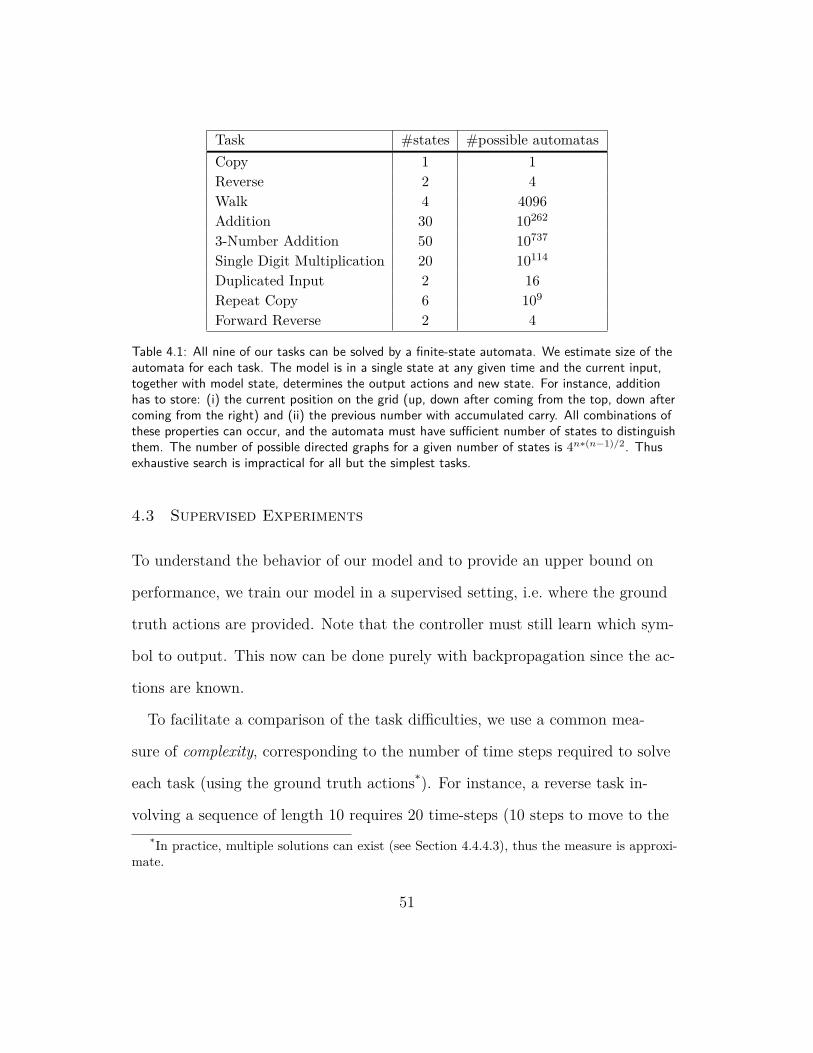
Task #states #possible automatasCopy 1 1Reverse 2 4Walk 4 4096Addition 30 10262

3-Number Addition 50 10737

Single Digit Multiplication 20 10114

Duplicated Input 2 16Repeat Copy 6 109

Forward Reverse 2 4

Table 4.1: All nine of our tasks can be solved by a finite-state automata. We estimate size of theautomata for each task. The model is in a single state at any given time and the current input,together with model state, determines the output actions and new state. For instance, additionhas to store: (i) the current position on the grid (up, down after coming from the top, down aftercoming from the right) and (ii) the previous number with accumulated carry. All combinations ofthese properties can occur, and the automata must have sufficient number of states to distinguishthem. The number of possible directed graphs for a given number of states is 4n∗(n−1)/2. Thusexhaustive search is impractical for all but the simplest tasks.

4.3 Supervised Experiments

To understand the behavior of our model and to provide an upper bound on

performance, we train our model in a supervised setting, i.e. where the ground

truth actions are provided. Note that the controller must still learn which sym-

bol to output. This now can be done purely with backpropagation since the ac-

tions are known.

To facilitate a comparison of the task difficulties, we use a common mea-

sure of complexity, corresponding to the number of time steps required to solve

each task (using the ground truth actions*). For instance, a reverse task in-

volving a sequence of length 10 requires 20 time-steps (10 steps to move to the*In practice, multiple solutions can exist (see Section 4.4.4.3), thus the measure is approxi-

mate.

51

“r” and 10 steps to move back to the start). The conversion factors between

the sequence lengths and the complexity are as follows: copy=1; reverse=2;

walk=1; addition=2; 3 row addition=3; single digit multiplication=1; duplicated

input=3; repeat copy=1; forward reverse=1.

For each task, we train a separate model, starting with sequences of complex-

ity 6 and incrementing by 4 once it achieves 100% accuracy on held-out exam-

ples of the current length. Training stops once the model successfully general-

izes to examples of complexity 1000. Three different cores for the controllers

are explored: (i) a 200 unit, 1-layer LSTM; (iii) a 200 unit, 1-layer GRU model

and (iii) a 200 unit, 1-layer feed-forward network. An additional linear layer is

placed on top of these models that maps the hidden state to either action for a

given interface, or the target symbol.

In Fig. 4.3 we show the accuracy of the different controllers the tasks such

as copy, reverse, walk, addition, 3-row addition and single digit multiplication.

We evaluate the model on test instances of increasing complexity, up to 20, 000

time-steps. The simple feed-forward controller generalizes perfectly on the copy,

reverse and walk tasks but completely fails on the remaining ones, due to a lack

of required memory†. The RNN-based controllers succeed to varying degrees,

although we observe some variability in performance.

Further insight can be obtained by examining the internal state of the con-†Amending the interfaces to allow both reading and writing on the same interface would

provide a mechanism for long-term memory, even with a feed-forward controller. However,then the same lack of generalization issues (encountered with more powerful controllers)would become an issue.

52

troller. To do this, we compute the autocorrelation matrix‡ A of the network

state over time when the model is processing a reverse task example of length

35, having been trained on sequences of length 10 or shorter. For this problem

there should be two distinct states: move right until “r” is reached and then

move left to the start. Table 4.2 plots A for models with three different con-

trollers. The larger the controller capacity, the less similar the states are within

the two phases of execution. This indicates that the larger the model becomes,

the underlaying learnt automata is driven further from the correct automata

that should have 2 states only. The figure also shows the confidence in the two

actions over time. In the case of high capacity models, the initial confidence in

the move left action is high, but this drops off after moving along the sequence.

This is because the controller has learned during training that it should change

direction after at most 10 steps. Consequently, the unexpectedly long test se-

quence makes it unsure of what the correct action is. By contrast, the simple

feed-forward controller does not show this behavior since it is stateless, and thus

has no capacity to know where it is within a sequence. The equivalent automata

is shown in Fig. 4.4(a), while Fig. 4.4(b) shows the incorrect time-dependent au-

tomata learned by the over-expressive RNN-based controllers. We note that this

argument is empirically supported by our results in Table 4.5, as well as related

work41,57 which found limited capacity controllers to be most effective. For ex-

ample, in the latter case, the counting and memorization tasks used controllers‡Let hi be the controller state at time i, then the autocorrelation Ai,j between time-

steps i and j is given by Ai,j =⟨hi−E,hj−E⟩

σ2 , i, j = 1, . . . , T where E =∑T

k=1 hk

T , σ2 =∑Tk=1⟨hk−E,hk−E⟩

T . T is the number of time steps (i.e. complexity).

53

with just 40 and 100 units respectively.

Walk Task

Figure 4.3: Test accuracy for several tasks with supervised actions over 10 runs for feed-forward(green), GRU (red) and LSTM (yellow) controllers. In this setting the optimal policy is providedduring training. The complexity is the number of time steps required to compute the solution. Ev-ery task has a slightly different conversion factor between the complexity and the sequence length:a complexity of 104 for copy and walk would mean 104 input symbols; for reverse would corre-spond to 104

2 input symbols; for addition would involve two 104

2 long numbers; for 3 row additionwould involve three 104

3 long numbers and for single digit multiplication would involve a single 104

long number.

4.4 No Supervision over actions

In the previous section, we assumed that the optimal controller actions were

given during training. This meant that only the output symbols need to be pre-

dicted and these could be learned via backpropagation. We now consider the

54

Auto

corr

elat

ion

mat

rixFeed-Forward Small LSTM Large LSTM

Table 4.2: Three models with different controllers (feed-forward, 200 unit LSTM and 400 unitLSTM) trained on the reverse task and applied to a 20 digit test example. The top row showsconfidence values for the two actions on the input tape: move left (green) and move right (red)as a function of time. The correct model should be equivalent to a two-state automata (Fig. 4.4),thus we expect to see the controller hidden state occupy two distinct values. The autocorrelationmatrices (whose axes are also time) show this to be the case for the feed-forward model – twodistinct blocks of high correlation. However, for the LSTM controllers, this structure is only looselypresent in the matrix, indicating that they have failed to learn the correct algorithm.

setting where the actions are also learned, in order to test the true capabili-

ties of the models to learn simple algorithms from pairs of input and output se-

quences. We present here two algorithms: REINFORCE, and Q-learning. There

are some tasks that we share between algorithms (copy and reverse). However,

we have used slightly different tasks to test each of algorithms.

4.4.1 Notation

We share notation between REINFORCE and Q-learning algorithm. This sec-

tion outlines the notation, which is simplified, and assumes that the environ-

ment is deterministic. However, neither REINFORCE nor Q-learning requires

55

right left

(a)

right1 right2 right3 right4 left

(b)

Figure 4.4: (a): The automata describing the correct solution to the reverse problem. The modelfirst has to go to the right while suppressing prediction. Then, it has to go to the left and predictwhat it sees at the given moment (this figure illustrates only actions over the Input Tape). (b)Another automata that solves the reverse problem for short sequences, but does not generalize toarbitrary length sequences, unlike (a). Expressive models like LSTMs tend to learn such incorrectautomata.

the environment to be deterministic.

Let A be a space of actions and S be the space of states. The execution of an

action in state s ∈ S causes it to transit to the new state s′ ∈ S, and provides a

reward r ∈ R. Some states are terminal and end the episode. We mark the time

steps of state, action and reward by t, i.e. at is an action at time t, st is the tth

state, and rt is the tth reward.

Our assumption on the environment being deterministic allows to associate

a state with a sequence of actions. An action a uniquely determines the transi-

tion s → s′. Therefore, the sequence of actions together with the initial state s0

dictates the state after the execution of the sequence of actions. Consequently,

st = (s0, a1, a2, . . . at). REINFORCE can be described as the function over se-

quences of actions, while Q-learning as the mapping from state-action space.

Nonetheless, they refer to similar objects as the sequence of actions is equivalent

to a state.

Let a1:t stand for a sequence of actions [a1, a2, . . . , at]. The cumulative future

reward is denoted by R(a1:T ), namely R(ak:T ) =∑T

t=k rt. Let pθ(at|a1:(t−1)) be

56

a parametric conditional probability of an action at given all previous actions

a1:(t−1). Finally, pθ is a policy parametrized by θ. Moreover, we use A† to de-

note the space of all sequences of actions that cause an episode to end. Let A‡

denote all valid subsequences of actions (i.e. A‡ ⊂ A†). Moreover, we define the

set of sequences of actions that are valid after executing a sequence a1:t and ter-

minate and denote it by: A†a1:t

. Every sequence a(t+1):T ∈ A†a1:t

terminates an

episode.

The Qp(s, a) function maps a pair of state and action to the cumulative fu-

ture reward under policy p. More formally, assuming that s = (s0, a1, . . . at),

then Qp(s, at+1) = R(t+1):T . Most of the time, we will skip the superscript p.

V is the value function and V (s) is the expected sum of future rewards start-

ing from the state s. Moreover, Q∗ and V ∗ are function values for the optimal

policy.

4.4.2 REINFORCE Algorithm

We present two reinforcement learning algorithms that we use in our setting:

REINFORCE and Q-learning. This section describes REINFORCE.

The REINFORCE algorithm directly optimizes the expected log probabil-

ity of the desired outputs, where the expectation is taken over all possible se-

quences of actions, weighted by the probability of taking these actions. Both

negative cross-entropy loss and REINFORCE loss maximize this objective. Neg-

ative cross-entropy maximizes the log probabilities of the model’s predictions,

while the REINFORCE loss deals with the probabilities of action sequences.

57

There are many other algorithms in discrete optimization that do not rely on

reinforcement learning, but that aim to optimize a similar quantity123,31,56,26.

The most successful approaches to discrete optimization require relaxation66.

However, relaxation techniques are problem specific, and cannot be applied

to arbitrary interfaces. Other techniques assume that the sequence of actions

is provided during training, such as DAGGER27 (DAGGER is considered an

imitation learning algorithm). Another algorithm like SEARN26 requires an

optimal policy for the training data, which we do not know. Fully general dis-

crete optimization algorithms end up being equivalent to the one considered in

reinforcement learning. For instance, various techniques in structural-output-

prediction construct sequences by iteratively taking the most likely action. Sim-

ilarly, Q-learning algorithm relies on picking the most likely actions. Therefore,

there is no significant difference between such approaches. The main issue with

applying classical structural prediction to our set of tasks is that the sequence of

actions that gives the highest reward is not the one that we look for (if we are

allowed to iterate over many action sequences for the same input). For instance,

it’s possible to solve addition without moving over the grid. The structural out-

put prediction approach could just find actions that produce targets without

looking on the input grid. Therefore, not committing to action and checking

its future outcome can have disastrous consequences. We lack a comparison of

performance for all structural-output-prediction and reinforcement learning al-

gorithms that have been considered in literature. However, we investigate two

specific reinforcement learning algorithms that have proven to work well in a

58

variety of domains. This section focuses on describing the objective of the RE-

INFORCE algorithm, and presents methods to optimize it.

The global objective can be written formally as:

∑[a1,a2,...,an]∈A†

preinforce(a1, a2, . . . , an|θ)[ n∑

i=1

log(pbp(yi|x1, . . . , xi, a1, . . . ai, θ)].

(4.1)

The probabilities in the above equation are parametrized with a neural network

(the controller). We have marked with preinforce the part of the equation which

is learned with REINFORCE. pbp indicates the part of the equation optimized

with the classical backpropagation.

interface Read Write Training Type

Input Tape Headwindow of values around

distribution over [−1, 0, 1] REINFORCEthe current position

Output TapeHead ∅ distribution over [0, 1] REINFORCE

Content ∅ distribution over output vocabulary Backpropagation

Memory TapeHead window of memory values around distribution over [−1, 0, 1] REINFORCE

Content the current address vector of real values to store Backpropagation

Miscellaneousall actions taken in ∅ ∅

the previous time step

Table 4.3: Table summarizes what the controller reads at every time step, and what it has to pro-duce. The “training” column indicates how the given part of the model is trained.

The controller receives a direct learning signal only when it decides to make

a prediction. If it chooses not to make a prediction at a given time step, it will

not receive a learning signal at the current time-step, but from the following

time-steps when a prediction is made. Theoretically, we can allow the controller

to run for an arbitrary number of steps without making any prediction, hop-

59

ing that after sufficiently many steps it will decide to make a prediction. Doing

so will also provide the controller with an arbitrary computational capability.

However, this strategy is both unstable and computationally infeasible. Thus,

we resort to limiting the total number of computational steps to a fixed upper

bound, and force the controller to predict the next desired output whenever the

number of remaining desired outputs is equal to the number of remaining com-

putational steps.

The goal of reinforcement learning is to maximize the sum of future rewards.

The REINFORCE algorithm139 does so directly by optimizing the parameters

of the policy pθ(at|a1:(t−1)). REINFORCE follows the gradient of the sum of the

future rewards. The objective function for episodic REINFORCE can be ex-

pressed as the sum over all sequences of valid actions that cause the episode to

end:

J(θ) =∑

[a1,a2,...,aT ]∈A†

pθ(a1, a2, . . . , aT )R(a1, a2, . . . , aT ) =∑

a1:T∈A†

pθ(a1:T )R(a1:T ).

(4.2)

This sum iterates over sequences of all possible actions, which is usually expo-

nential in size or even infinite, so it cannot be computed exactly and cheaply for

most of problems. However, it can be written as an expectation, which can be

approximated with an unbiased estimator. We have that:

60

J(θ) =∑

a1:T∈A†

pθ(a1:T )R(a1:T ) = (4.3)

Ea1:T∼pθ

n∑t=1

r(a1:t) = (4.4)

Ea1∼pθ(a1)Ea2∼pθ(a2|a1) . . .EaT∼pθ(aT |a1:(T−1))

T∑t=1

r(a1:t). (4.5)

The last expression suggests a procedure to estimate J(θ): simply sequentially

sample each at from the model distribution pθ(at|a1:(t−1)) for t from 1 to T . The

unbiased estimator of J(θ) is the sum of r(a1:t) and this gives us an algorithm

to estimate J(θ). However, the main interest is in training a model maximizing

this quantity.

The REINFORCE algorithm maximizes J(θ) by following its gradient:

∂θJ(θ) =∑

a1:T∈A†

[∂θpθ(a1:T )

]R(a1:T ). (4.6)

However, the above expression is a sum over the set of the possible action se-

quences, so it cannot be computed directly for most A†. Once again, the RE-

INFORCE algorithm rewrites this sum as an expectation that is approximated

with sampling. It relies on the following equation: ∂θf(θ) = f(θ)∂θf(θ)f(θ)

= f(θ)∂θ[log f(θ)].

This identity is valid as long as f(x) = 0. As typical neural network parametriza-

tions of distributions assign non-zero probability to every action, this condition

holds for f = pθ. We have that:

61

∂θJ(θ) =∑

[a1:T ]∈A†

[∂θpθ(a1:T )

]R(a1:T ) = (4.7)

=∑

a1:T∈A†

pθ(a1:T )[∂θ log pθ(a1:T )

]R(a1:T ) (4.8)

=∑

a1:T∈A†

pθ(a1:T )[ n∑

t=1

∂θ log pθ(ai|a1:(t−1))]R(a1:T ) (4.9)

= Ea1∼pθ(a1)Ea2∼pθ(a2|a1) . . .EaT∼pθ(aT |a1:T−1)

[ T∑t=1

∂θ log pθ(ai|a1:(t−1))][ T∑

t=1

r(a1:t)].

(4.10)

The last expression gives us an algorithm for estimating ∂θJ(θ), which we sketch

on the left side of the Figure 4.6. It is easiest to describe it with respect to the

computational graph behind a neural network. REINFORCE can be imple-

mented as follows. The neural network first outputs: lt = log pθ(at|a1:(t−1)).

Then, we sequentially sample an action at from the distribution elt , and execute

the sampled action at. Simultaneously, we experience a reward r(a1:t). Now,

backpropagate the sum of the rewards∑T

t=1 r(a1:t) to every node ∂θ log pθ(at|a1:(t−1)).

We have derived an unbiased estimator for the sum of future rewards, and the

unbiased estimator of its gradient. However, the derived gradient estimator has

high variance, which makes learning difficult. This model employs several tech-

niques to reduce the gradient estimator variance: (1) future rewards backprop-

agation, (2) online baseline prediction, and (3) offline baseline prediction. All

these techniques are crucial to solve our tasks. More information can be found

in Section 4.4.2.1.

Finally, we need a way of verifying the correctness of our implementation. We

62

discovered a technique that makes it possible to easily implement a gradient

checker for nearly any model that uses REINFORCE. Section 4.4.2.2 describes

this technique. Finally, some tasks were significantly simpler with a modified

controller, described in Section 4.4.2.3.

4.4.2.1 Variance reduction

We had to employ several techniques to decrease the variance of gradients dur-

ing learning with REINFORCE. Here we outline these techniques.

4.4.2.1.1 Causality of actions

The actions at time t cannot influence rewards obtained in the past, as the

past rewards are caused by actions prior to them. This idea allows to derive an

unbiased estimator of ∂θJ(θ) with lower variance. Here, we formalize it:

63

∂θJ(θ) =∑

a1:T∈A†

pθ(a)[∂θ log pθ(a)

]R(a) (4.11)

=∑

a1:T∈A†

pθ(a)[∂θ log pθ(a)

][ T∑t=1

r(a1:t)]

(4.12)

=∑

a1:T∈A†

pθ(a)[ T∑

t=1

∂θ log pθ(a1:t)r(a1:t)]

(4.13)

=∑

a1:T∈A†

pθ(a)[ T∑

t=1

∂θ log pθ(a1:t)r(a1:t) + ∂θ log pθ(a(t+1):T |a1:t)r(a1:t)](4.14)

=∑

a1:T∈A†

T∑t=1

pθ(a1:t)∂θ log pθ(a1:t)r(a1:t) + pθ(a)∂θ log pθ(a(t+1):T |a1:t)r(a1:t)

(4.15)

=∑

a1:T∈A†

T∑t=1

pθ(a1:t)∂θ log pθ(a1:t)r(a1:t) + pθ(a1:t)r(a1:t)∂θpθ(a(t+1):T |a1:t)

(4.16)

=∑

a1:T∈A†

[ T∑t=1

pθ(a1:t)∂θ log pθ(a1:t)r(a1:t)]+∑

a1:T∈A†

T∑t=1

[pθ(a1:t)r(a1:t)∂θpθ(a(t+1):T |a1:t)

].

(4.17)(4.18)

We will show that the right side of this equation is equal to zero, because the

future actions a(t+1):T do not influence past rewards r(a1:t). Here we formalize

it, using the identity Ea(t+1):T∈A†a1:t

pθ(a(t+1):T |a1:t) = 1:

64

∑a1:T∈A†

T∑t=1

[pθ(a1:t)r(a1:t)∂θpθ(a(t+1):T |a1:t)

]= (4.19)

∑a1:t∈A‡

[pθ(a1:t)r(a1:t)

∑a(t+1):T∈A†

a1:t

∂θpθ(a(t+1):T |a1:t)]= (4.20)

∑a1:t∈A‡

pθ(a1:t)r(a1:t)∂θ1 = 0. (4.21)

We can purge the right side of the equation for ∂θJ(θ):

∂θJ(θ) =∑

a1:T∈A†

[ T∑t=1

pθ(a1:t)∂θ log pθ(a1:t)r(a1:t)]

(4.22)

= Ea1∼pθ(a)Ea2∼pθ(a|a1) . . .EaT∼pθ(a|a1:(T−1))

[ T∑t=1

∂θ log pθ(at|a1:(t−1))T∑i=t

r(a1:i)]

(4.23)

The last line of derived equations describes the learning algorithm with a

smaller variance than the original REINFORCE algorithm.

4.4.2.1.2 Online baseline prediction

Online baseline prediction is the idea that the importance of the reward is

determined by its relative relation to other rewards. All the rewards could be

shifted by a constant factor and this change should not affect its relation; thus,

it should not influence the expected gradient. However, it could decrease the

variance of the gradient estimate.

The aforementioned shift is called the baseline, and it can be estimated sepa-

rately for every time step. We have that:

65

∑a(t+1):T∈A†

a1:t

pθ(a(t+1):T |a1:t) = 1 (4.24)

∂θ∑

a(t+1):T∈A†a1:t

pθ(a(t+1):T |a1:t) = 0. (4.25)

(4.26)

We can subtract the above quantity (multiplied by bt) from our estimate of the

gradient without changing its expected value:

∂θJ(θ) = Ea1∼pθ(a)Ea2∼pθ(a|a1) . . .EaT∼pθ(a|a1:(T−1))

[ T∑t=1

∂θ log pθ(at|a1:(t−1))T∑i=t

(r(a1:i)− bt)].

(4.27)

The above statement holds for any sequence bt, and we aim to find the sequence

bt that yields the lowest variance estimator on ∂θJ(θ). The variance of our esti-

mator is:

V ar = Ea1∼pθ(a)Ea2∼pθ(a|a1) . . .EaT∼pθ(a|a1:(T−1))

[ T∑t=1

∂θ log pθ(at|a1:(t−1))T∑i=t

(r(a1:i)− bt)]2−

(4.28)[Ea1∼pθ(a)Ea2∼pθ(a|a1) . . .EaT∼pθ(a|a1:(T−1))

[ T∑t=1

∂θ log pθ(at|a1:(t−1))T∑i=t

(r(a1:i)− bt)]]2

(4.29)

The second term does not depend on bt and the variance is always positive.

Hence, it suffices to minimize the first term, which is minimal when its deriva-

tive with respect to bt is zero. This implies the following:

66

Ea1∼pθ(a)Ea2∼pθ(a|a1) . . .EaT∼pθ(a|a1:(T−1))

T∑t=1

∂θ log pθ(at|a1:(t−1))T∑i=t

(r(a1:i)− bt) = 0

(4.30)T∑t=1

∂θ log pθ(at|a1:(t−1))T∑i=t

(r(a1:i)− bt) = 0 (4.31)

bt =

∑Tt=1 ∂θ log pθ(at|a1:(t−1))

∑Ti=t r(a1:t)∑T

t=1 ∂θ log pθ(at|a1:(t−1))(4.32)

This gives us an estimate for a vector bt ∈ R#θ (where #θ is the number of

dimensions of theta). However, it is common to use a single scalar for bt ∈ R,

and estimate it as Epθ(at:T |a1:(t−1))R(at:T ).

4.4.2.1.3 Offline baseline prediction

The REINFORCE algorithm works much better when it has accurate base-

lines. A separate LSTM can help in the baseline estimation. This can be done

by first running the baseline LSTM on the entire input tape to produce a vec-

tor summarizing the input. Next, continue running the baseline LSTM in tan-

dem with the controller LSTM, so that the baseline LSTM receives precisely the

same inputs as the controller LSTM, and outputs a baseline bt at each time step

t. The baseline LSTM is trained to minimize∑T

t=1

[R(at:T ) − bt

]2 (Fig. 4.5).

This technique introduces a biased estimator; however, it works well in practice.

We found it important to first have the baseline LSTM go over the entire in-

put before computing the baselines bt. This is especially beneficial whenever

there is considerable variation in the difficulty of the examples. For example, if

the baseline LSTM can recognize that the current instance is unusually difficult,

67

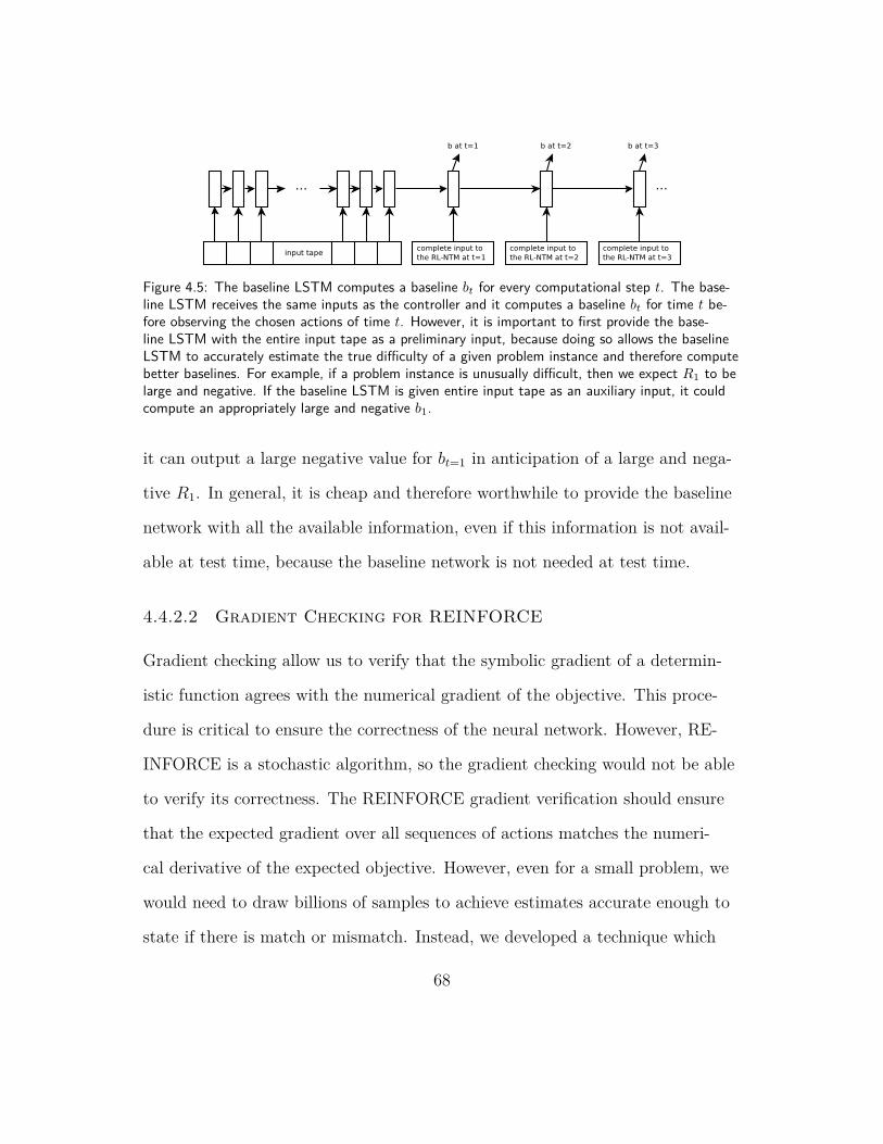
Figure 4.5: The baseline LSTM computes a baseline bt for every computational step t. The base-line LSTM receives the same inputs as the controller and it computes a baseline bt for time t be-fore observing the chosen actions of time t. However, it is important to first provide the base-line LSTM with the entire input tape as a preliminary input, because doing so allows the baselineLSTM to accurately estimate the true difficulty of a given problem instance and therefore computebetter baselines. For example, if a problem instance is unusually difficult, then we expect R1 to belarge and negative. If the baseline LSTM is given entire input tape as an auxiliary input, it couldcompute an appropriately large and negative b1.

it can output a large negative value for bt=1 in anticipation of a large and nega-

tive R1. In general, it is cheap and therefore worthwhile to provide the baseline

network with all the available information, even if this information is not avail-

able at test time, because the baseline network is not needed at test time.

4.4.2.2 Gradient Checking for REINFORCE

Gradient checking allow us to verify that the symbolic gradient of a determin-

istic function agrees with the numerical gradient of the objective. This proce-

dure is critical to ensure the correctness of the neural network. However, RE-

INFORCE is a stochastic algorithm, so the gradient checking would not be able

to verify its correctness. The REINFORCE gradient verification should ensure

that the expected gradient over all sequences of actions matches the numeri-

cal derivative of the expected objective. However, even for a small problem, we

would need to draw billions of samples to achieve estimates accurate enough to

state if there is match or mismatch. Instead, we developed a technique which

68

avoids sampling and allows for gradient verification of REINFORCE within sec-

onds on a laptop.

REINFORCE Gradient Checking of REINFORCE

Figure 4.6: Figure sketches algorithms: (Left) the REINFORCE algorithm, (Right) gradientchecking for the REINFORCE algorithm. The red color indicates necessary steps to override theREINFORCE to become the gradient checker for the reinforce.

First, we have to reduce the size of our task to make sure that the number

of possible actions is manageable (e.g., < 104). This is similar to conventional

gradient checkers, which can only be applied to small models. Next, we enumer-

ate all possible sequences of actions that terminate the episode (brute force). By

definition, these are precisely all the elements of A†.

The key idea is the following: we override the sampling function with a deter-

ministic function that returns every possible sequence of actions once (this are

sequences from A†). This deterministic sampler records the probability of the

every sequence and modifies REINFORCE to account for it.

For efficiency, it is desirable to use a single minibatch whose size is #A†. The

sampling function needs to be adapted in a way that incrementally outputs the

appropriate sequence from A† as we repeatedly call the sampling function. At

the end of the minibatch, the sampling function will have access to the total

69

probability of each action sequence (∏

t pθ(at|a1:t−1)), which in turn can be used

to exactly compute J(θ) and its derivative. To compute the derivative, the RE-

INFORCE gradient produced by each sequence a1:T ∈ A† should be weighted by

its probability pθ(a1:T ). We summarize this procedure in Figure 4.6.

The gradient checking is critical for ensuring the correctness of our imple-

mentation. While the basic REINFORCE algorithm is conceptually simple, our

model is fairly complicated, as REINFORCE is used to train several interfaces

of our model. Moreover, the model uses three separate techniques for reducing

the variance of the gradient estimators. The model’s high complexity greatly in-

creases the probability of a code error. In particular, our early implementations

were incorrect, and we were able to fix them only after implementing gradient

checking.

4.4.2.3 Direct Access Controller

All tasks considered by the REINFORCE algorithm involve rearranging the in-

put symbols in some way. For example, a typical task is to reverse a sequence

(Section 4.2 lists the tasks). For these tasks, the controller would benefit from

a built-in mechanism to directly copy an appropriate input to memory and to

output. Such a mechanism would free the LSTM controller from remembering

the input symbol in its control variables (“registers”), and would shorten the

backpropagation paths and therefore make learning easier. We implemented

this mechanism by adding the input to the memory and to the output, while

also adding the memory to the output and to the adjacent memories (Fig. 4.8),

70

and adjust these additive contributions by a dynamic scalar (sigmoid) computed

from the controller’s state. This way, the controller can decide to effectively not

add the current input to the output at a given time step. Unfortunately, the ne-

cessity of this architectural modification is a drawback of our implementation,

since it is not domain independent and would therefore not improve the perfor-

mance of the model on many tasks of interest.

Figure 4.7: LSTM as a controller.Figure 4.8: The direct access con-troller.

4.4.3 Q-learning

We present two reinforcement learning algorithms used in our setting: REIN-

FORCE (Section 4.4.2), and Q-learning. This section describes Q-learning.

The purpose of reinforcement learning is to learn a policy that yields the

highest sum of future rewards. Q-learning does it indirectly by learning a Q-

function. Q(s, a) is a function that maps a pair of state and action to the sum

of future rewards. This function is parametrized by the neural network and

is learned. The optimal policy can then be extracted by taking argmax over

Q(s, •).

The function Q is updated during training according to:

71

Qt+1(s, a) = Qt(s, a)− α[Qt(s, a)−

(R(s′) + γmax

aQn(s

′, a))]. (4.33)

Taking the action a in state s causes a transition to state s′, which in our case

is deterministic. R(s′) is the reward experienced in state s′, γ is the discount

factor and α is the learning rate. Another commonly considered quantity is

V (s) = maxa Q(s, a). V is the value function, and V (s) is the expected sum of

future rewards starting from state s. Moreover, Q∗ and V ∗ are function values

for the optimal policy.

Our controller receives a reward of 1 every time it correctly predicts a digit

(and 0 otherwise). Since the overall solution to the task requires all digits to

be correct, we terminate a training episode as soon as an incorrect prediction is

made. This learning environment is non-stationary, since even if the model ini-

tially picks the right actions, the symbol prediction is unlikely to be correct and

the model receives no reward. But further on in training, when the symbol pre-

diction is more reliable, the correct action will be rewarded§. This is important

because reinforcement learning algorithms assume stationarity of the environ-

ment, which is not true in our case. Learning in non-stationary environments is

not well understood and there are no definitive methods to deal with it. How-

ever, empirically we find that this non-stationarity can be partially addressed by

the use of Watkins Q(λ)133, as detailed in Section 4.4.3.2.§If we were to use reinforcement to train the symbol output as well as the actions, then

the environment would be stationary. However, this would mean ignoring the reliable signalavailable from direct backpropagation of the symbol output.

72

4.4.3.1 Dynamic Discount

Various episodes differ significantly in terms of length and thus they differ in

terms of the sum of the future rewards as well. The initial state is insufficient

to predict the sum of the future rewards when the length is unknown. More-

over, shifting or scaling Q induces the same policy. We propose to dynami-

cally rescale Q so (i) it is independent of the length of the episode and (ii) Q

is within a small range, making it easier to predict.

We define Q to be our reparametrization and Q(s, a) should be roughly in the

range [0, 1], and it should correspond to how close we are to V ∗(s). Q could be

decomposed multiplicatively as Q(s, a) = Q(s, a)V ∗(s). However, in practice, we

do not have access to V ∗(s), so instead we use an estimate of the future rewards

based on the total number of digits left in the sequence. Since every correct pre-

diction yields a reward of 1, the optimal policy should be that the sum of future

rewards be equal to the number of remaining symbols to predict. The number

of remaining symbols to predict is known and we denote it by V (s). We remark

that this is a form of supervision, albeit a weak one.

Therefore, we normalize the Q-function by the remaining sum of rewards left

in the task:

Q(s, a) :=Q(s, a)

V (s). (4.34)

We assume that s transitions to s′, and we re-write the Q-learning update equa-

tions:

73

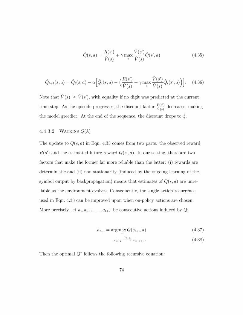
Q(s, a) =R(s′)

V (s)+ γmax

a

V (s′)

V (s)Q(s′, a) (4.35)

Qt+1(s, a) = Qt(s, a)− α[Qt(s, a)−

(R(s′)

V (s)+ γmax

a

V (s′)

V (s)Qt(s

′, a))]

. (4.36)

Note that V (s) ≥ V (s′), with equality if no digit was predicted at the current

time-step. As the episode progresses, the discount factor V (s′)

V (s)decreases, making

the model greedier. At the end of the sequence, the discount drops to 12.

4.4.3.2 Watkins Q(λ)

The update to Q(s, a) in Eqn. 4.33 comes from two parts: the observed reward

R(s′) and the estimated future reward Q(s′, a). In our setting, there are two

factors that make the former far more reliable than the latter: (i) rewards are

deterministic and (ii) non-stationarity (induced by the ongoing learning of the

symbol output by backpropagation) means that estimates of Q(s, a) are unre-

liable as the environment evolves. Consequently, the single action recurrence

used in Eqn. 4.33 can be improved upon when on-policy actions are chosen.

More precisely, let at, at+1, . . . , at+T be consecutive actions induced by Q:

at+i = argmaxa

Q(st+i, a) (4.37)

st+iat+i−−→ st+i+1. (4.38)

Then the optimal Q∗ follows the following recursive equation:

74

Q∗(st, at) =T∑i=1

γi−1R(st+i) + γT maxa

Q∗(st+n+1, a). (4.39)

and the update rule corresponding to Eqn. 4.33 becomes:

Qt+1(st, at) = Qt(st, at)− α[Qt(st, at)−

( T∑i=1

γi−1R(st+i) + γT maxa

Qt(st+n+1, a))].

(4.40)

This is a special form of Watkins Q(λ)133 where λ = 1. The classical applica-

tions of Watkins Q(λ) suggest choosing a small λ, which is a trade off on es-

timates based on various numbers of future rewards. λ = 0 rolls back to the

classical Q-learning. Due to the reliability of our rewards, we found λ = 1 to be

better than λ < 1; however, this needs further study.

We remark that this unrolling of rewards can only take place until a non-

greedy action is taken. When using an ϵ-greedy policy, we expect to be able to

unroll ϵ−1 steps on average. For the value of ϵ = 0.05 used in our experiments

this corresponds to 20 steps on average.

4.4.3.3 Penalty on Q-function

After reparametrizing the Q-function to Q (Section 4.4.3.1), the optimal Q∗(s, a)

should be 1 for the correct action and 0 otherwise. To encourage our estimate

Q(s, a) to converge to this, we introduce a penalty that “pushes down” on in-

correct actions: κ∥∑

a Q(s, a) − 1∥2. Therefore, it influences the value of Q for

actions that are taken infrequently. This has the effect of introducing a margin

75

between correct and incorrect actions, which greatly improves generalization.

We commence training with κ = 0 and make it non-zero once good accuracy is

reached on short samples (introducing it from the outset hurts learning).

4.4.4 Experiments

REINFORCE and Q-learning experiments have been conducted during separate

periods, and on different set of tasks. REINFORCE tasks involve rearrange-

ment of symbols, while Q-learning experiments are mainly about arithmetics.

Nonetheless, they share the reverse and copy tasks. We have trained REIN-

FORCE on the following tasks: Copy, Reverse, Duplicated Input, Repeat Copy,

Forward Reverse, and Q-learning on Copy, Reverse, Walk, Addition, 3-Number

Addition and Single Digit Multiplication. We start by presenting results from

the REINFORCE algorithm.

4.4.4.1 Experiments with REINFORCE algorithm

TaskController LSTM Direct Access

Copy Duplicated Input Reverse × Forward Reverse × Repeat Copy ×

Table 4.4: Success of training on various tasks for a given controller.

This section presents results from training our model on REINFORCE algo-

rithm Table 4.4. We trained our model using SGD with a fixed learning rate

of 0.05 and a fixed momentum of 0.9. We used a batch of size 200, which we

found to work better than smaller batch sizes (such as 50 or 20). We normal-

76

ized the gradient by batch size and not by sequence length. We independently

clip the norm of the gradients w.r.t. the model parameters to 5, and the gradi-

ent w.r.t. the baseline network to 2. We initialize the controller and the base-

line model using a Gaussian with standard deviation 0.1. We used an inverse

temperature of 0.01 for the different action distributions. Doing so reduced the

effective learning rate of the REINFORCE derivatives. The memory consists of

35 real values through which we backpropagate. The initial memory state and

the controller’s initial hidden states were set to the zero vector.

The Forward Reverse task is particularly interesting. In order to solve the

problem, the controller has to move to the end of the sequence without mak-

ing any predictions. While doing so, it has to store the input sequence into its

memory (encoded in real values), and use its memory when reversing the se-

quence (Fig. 4.9).

We have also experimented with a number of additional tasks but with less

empirical success. Tasks we found to be too difficult include sorting, long inte-

ger addition (in base 3 for simplicity), and Repeat Copy when the input tape is

forced to only move forward. While we were able to achieve reasonable perfor-

mance on the sorting task, the controller learned an ad-hoc algorithm and made

excessive use of its controller memory in order to sort the sequence.

Empirically, we found all components of the model essential to successfully

solving these problems. All our tasks are either solvable in under 20, 000 param-

eter updates or fail in arbitrary number of updates. We were completely unable

to solve Repeat Copy, Reverse, and Forward reverse with the LSTM controller,

77

Reverse Duplicated Input

Repeat Copy Forward Reverse

Figure 4.9: This figure presents the execution traces from experiments with REINFORCE. Thevertical depicts execution time. The rows show the input pointer, output pointer, and memorypointer (with the ∗ symbol) at each step of the controller’s execution. Note that we represent theset 1, . . . , 30 with 30 distinct symbols, and lack of prediction with #.

78

but we succeeded with a direct access controller. Moreover, we were also unable

to solve any of these problems at all without a curriculum (except for short se-

quences of length 5).

4.4.4.2 Experiments with Q-learning

This section presents the results of the Q-learning algorithm. We apply our en-

hancements to the six tasks in a series of experiments designed to examine the

contribution of each of them. Unless otherwise specified, the controller is a 1-

layer GRU model with 200 units. This was selected on the basis of its mean

performance across the six tasks in the supervised setting (see Section 4.3). As

the performance of reinforcement learning methods tend to be highly stochas-

tic, we repeated each experiment 10 times with a different random seed. Each

model is trained using 3 × 107 characters which takes ∼ 4 hrs. A model is con-

sidered to have successfully solved the task if it is able to give a perfect answer

to 50 test instances, each 100 digits in length. The GRU model is trained with

a batch size of 20, a learning rate of α = 0.1, using the same initialization36 but

multiplied by 2. All tasks are trained with the same curriculum used in the su-

pervised experiments57, whereby the sequences are initially of complexity 6 (cor-

responding to 2 or 3 digits, depending on the task) and once 100% accuracy is

achieved, increased by 4 until the model is able to solve validation sequences of

length 100. For 3-row addition, a more elaborate curriculum was needed which

started with examples that did not involve a carry and contained many zero.

The test distribution was unaffected.

79

Test length 100 100 100 100 100 100 100 100 1000 1000#Units 600 400 200 200 200 200 200 200 200 200Discount γ 1 1 1 0.99 0.95 D D D D DWatkins Q(λ) × × × × × ×

Task Penalty × × × × × × × × Copying 30% 60% 90% 50% 70% 90% 100% 100% 100% 100%Reverse 0% 0% 0% 0% 0% 0% 0% 0% 0% 0%Reverse (FF controller) 0% 0% 0% 0% 0% 0% 100% 90% 100% 90%Walk 0% 0% 0% 0% 0% 0% 10% 90% 10% 80%Walk (FF controller) 0% 0% 0% 0% 0% 0% 100% 100% 100% 100%2-row Addition 10% 70% 70% 70% 80% 60% 60% 100% 40% 100%3-row Addition 0% 0% 0% 0% 0% 0% 0% 0% 0% 0%3-row Addition (extra curriculum) 0% 50% 80% 40% 50% 50% 80% 80% 10% 60%Single Digit Multiplication 0% 0% 0% 0% 0% 100% 100% 100% 0% 0%

Table 4.5: Success rates for classical Q-learning (columns 2-5) versus our enhanced Q-learning. AGRU-based controller is used on all tasks, except reverse and walk which use a feed-forward net-work. Curriculum learning was also used for the 3-row addition task (see text for details). Whendynamic discount (D), Watkins Q(λ) and the penalty term are all used, the model consistentlysucceeds on all tasks. The model still performs well on test sequences of length 1000, apart fromthe multiplication task. Increasing the capacity of the controller results in worse performance(columns 2-4).

We show results for various combinations of terms in Table 4.5. The experi-

ments demonstrate that standard Q-learning fails on most of our tasks (first six

columns). Each of our additions (dynamic discount, Watkins Q(λ) and penalty

term) give significant improvements. When all three are used, our model is able

to succeed at all tasks, provided that the appropriate curriculum and controller

are used. Remark: there is not a single model that succeed on all tasks, but for

every task we have a model that succeeds on it (i.e. compare Reverse with Re-

verse with FF controller in Table 4.5).

For the reverse and walk tasks, the default GRU controller failed completely.

However, using a feed-forward controller instead enabled the model to succeed,

when dynamic discount and Watkins Q(λ) were used. As noted above, the 3-

row addition required a more careful curriculum before the model was able to

80

(FF) (FF)

Figure 4.10: Test accuracy as a function of task complexity (10 runs) for standard Q-learning(blue) and our enhanced version (dynamic discount, Watkins Q(λ) and penalty term). Accuracycorresponds to the fraction of correct test cases (all digits must be predicted correctly for the in-stance to be considered correct).

learn successfully. Increasing the capacity of the controller (columns 2-4) hurts

performance, echoing Table 4.2. The last two columns of Table 4.5 show the

results on test sequences of length 1000. Except for multiplication, the models

still generalized successfully.

Fig. 4.10 shows accuracy as a function of test example complexity for stan-

dard Q-learning and our enhanced version. The difference in performance is

clear. At very high complexity, corresponding to thousands of digits, the ac-

curacy starts to drop on the more complicated tasks. We note that these trends

are essentially the same as those observed in the supervised setting (Fig. 4.3),

81

suggesting that Q-learning is not at fault. Instead, the inability of the controller

to learn an automata seems to be the cause. Potential solutions to this might

include (i) noise injection, (ii) discretization of state, (iii) a state error correc-

tion mechanism or (iv) regularizing the learned automata using MDL principles.

However, the issue of the inability of RNN to perfectly represent an automata

can be examined separately from the setting where actions have to be learned

(i.e. in the supervised domain).

4.4.4.3 Multiple Solutions

On examining the models learned on the addition task, we notice that three dif-

ferent solutions were discovered. While they all give the correct answer, they

differ in their actions over the input grid, as shown in Fig. 4.11.

Figure 4.11: Our model found three different solutions to the addition task, all of which give thecorrect answer. The arrows show the trajectory of the read head over the input grid.

4.5 Discussion

We have explored the ability of neural network models to learn algorithms for

symbol rearrangement and simple arithmetic operations. Through experiments

with supervision and reinforcement learning, we have shown that they can do

this successfully, albeit with caveats. Solving problems with small Kolmogorov

complexity is not interesting on its own because any developer could write down

82

such solutions explicitly. However, being able to train neural networks to ex-

press the correct solution to such problems is the prerequisite to finding small

Kolmogorov complexity solutions to more complicated problems.

Next chapter takes the opposite route to the approach presented in this chap-

ter. We attempt to identify smaller building blocks, rather than providing a

new high abstraction interface. Such small blocks allow us to rediscover known

algorithms such as convolution.

83

5Learning the convolution algorithm

Chapter 4 presents methods to extend neural networks by specifying interfaces

that can easily express certain algorithms. However, the interfaces considered

may provide abstractions that are too high-level. Consider the following anal-

ogy, in order to build a complicated LEGO structure, one needs many small

bricks, rather than a few large ones. While having a variety of large bricks al-

lows to rapidly build some structures, large bricks may be insufficient to build

interesting LEGO structures. By the same token, having many high-level inter-

faces allows to solve a great variety of tasks, but such interfaces may be inade-

quate to solve needed tasks. We are interested in finding the smallest metaphor-

84

ical building blocks that are sufficient to express certain high-level concepts of

interest. One such high-level concept that we could learn is convolution. In this

chapter, we attempt to rediscover the high-level concept of convolution. This

chapter is based on the ICLR 2014 paper “Spectral networks and locally con-

nected networks on graphs”15 and was done in collaboration with Joan Bruna,

Arthur Szlam and Yann LeCun.

Convolutional neural networks (CNN) have proven successful in various com-

puter vision tasks like object recognition76,67,108, video classification124,73 and

others. CNNs have significantly lower Kolmogorov complexity than fully con-

nected networks due to requiring a smaller number of parameters to solve the

same task. CNNs exploit several structures that reduce the number of parame-

ters:

1. The translation structure, which allows the use of filters instead of generic

linear maps and, hence enables weight sharing.

2. The metric of the grid, which allows compactly supported filters, whose

support is typically much smaller than the size of the input signals.

3. The multiscale dyadic clustering of the grid, which allows subsampling

implemented using strided convolutions and pooling.

Consider a layer on a d-dimensional grid of n input coordinates. A fully con-

nected layer with m outputs requires n · m parameters, which in typical oper-

ating regimes amounts to a complexity of O(n2) parameters. Using arbitrary

filters instead of generic fully connected layers reduces the complexity to O(n)

85

parameters per feature map, as does using the metric structure by building a

“locally connected” network43,72. Using both together further reduces the com-

plexity to O(k · S) parameters, where k is the number of feature maps and S is

the support of the filters. As a result, the learning complexity is independent of

n. Finally, using the multiscale dyadic clustering allows each successive layer to

use a factor of 2d fewer (spatial) coordinates per filter.

We rediscover convolution by considering classification problem in a more

complex domain than a 2-D grid. Graphs offer a natural framework to gener-

alize the low-dimensional structure of a grid. For instance, data defined on 3-D

meshes, such as surface tension, temperature, measurements from a network of

meteorological stations, or data coming from social networks or collaborative fil-

tering, are all examples of structured input defined on graphs. Another relevant

example is the intermediate representation arising from deep neural networks.

Although the spatial convolutional structure can be exploited at several layers,

typical CNN architectures do not assume any geometry in the “feature” dimen-

sion, resulting in 4-D tensors which are only convolutional along their spatial

coordinates.

In this work, we discuss constructions of deep neural networks on graphs

other than regular grids. We propose two different constructions. In the first

one, we show that one can extend properties (2) and (3) to general graphs, and

use them to define “locally” connected and pooling layers, which require O(n)

parameters instead of O(n2). We define this to be the spatial construction. The

other construction, which we call spectral construction, draws on the proper-

86

ties of convolutions in the Fourier domain. In Rd, convolutions are linear op-

erators diagonalised by the Fourier basis exp(iω · t), where ω, t ∈ Rd. One

may then extend convolutions to general graphs by finding the corresponding

“Fourier” basis. This equivalence is given by the graph Laplacian, an opera-

tor which enables harmonic analysis on the graphs6. The spectral construction

needs at most O(n) parameters per feature map, and also enables a construc-

tion where the number of parameters is independent of the input dimension n.

These constructions allow efficient forward propagation and can be applied to

datasets with a very large number of coordinates.

Our main contributions are summarized as follows:

• We show that from a weak geometric structure in the input domain, it is

possible to obtain efficient architectures using O(n) parameters, which we

validate on low-dimensional graph datasets.

• We introduce a construction using O(1) parameters which we empirically

verify, and discuss its connections with harmonic analysis on graphs.

5.1 Spatial Construction

The most immediate generalization of CNN to general graphs is to consider

multiscale, hierarchical, local receptive fields, as suggested in20. For that pur-

pose, the grid will be replaced by a weighted graph G = (Ω,W ), where Ω is a

discrete set of size m and W is a m×m symmetric and nonnegative matrix.

87

5.1.1 Locality via W

The notion of locality can be generalized easily in the context of a graph. In-

deed, the weights in a graph determine a notion of locality. For example, a

straightforward way to define neighborhoods on W is to set a threshold δ > 0

and take neighborhoods

Nδ(j) = i ∈ Ω : Wij > δ .

We can restrict attention to sparse “filters” with receptive fields given by these

neighborhoods to get locally connected networks, thus reducing the number of

parameters in a filter layer to O(S · n), where S is the average neighborhood

size.

5.1.2 Multiresolution Analysis on Graphs

CNNs reduce the size of the grid via pooling and subsampling layers. These lay-

ers are possible because of the natural multiscale clustering of the grid: they

input all feature maps over a cluster, and output a single feature for that clus-

ter. On the grid, the dyadic clustering behaves nicely with respect to the met-

ric and the Laplacian (and similarly with the translation structure). There is

a large literature on forming multiscale clusterings on graphs, see for exam-

ple62,69,131,30. Finding multiscale clusterings that are provably guaranteed to

behave well w.r.t. the Laplacian on the graph is still an open area of research.

In this work we will use a naive agglomerative method.

88

Figure 5.1 illustrates a multiresolution clustering of a graph with the corre-

sponding neighborhoods.

Figure 5.1: Undirected Graph G = (Ω0,W ) with two levels of clustering. The original points aredrawn in gray.

5.1.3 Deep Locally Connected Networks

The spatial construction starts with a multiscale clustering of the graph, similar

to20. We consider K scales. We set Ω0 = Ω, and for each k = 1 . . . K, we de-

fine Ωk, a partition of Ωk−1 into dk clusters; and a collection of neighborhoods

around each element of Ωk−1:

Nk = Nk,i ; i = 1 . . . dk−1 .

Now we can define the k-th layer of the network. We assume without loss of

generality that the input signal is a real signal defined in Ω0, and we denote by

fk the number of “filters” created at each layer k. Each layer of the network will

89

transform a fk−1-dimensional signal indexed by Ωk−1 into a fk-dimensional sig-

nal indexed by Ωk, thus trading-off spatial resolution with newly created feature

coordinates.

More formally, if xk = (xk,i ; i = 1 . . . fk−1) is the dk−1 × fk−1 is the input to

layer k, its output xk+1 is defined as

xk+1,j = Lkh

(fk−1∑i=1

Fk,i,jxk,i

)(j = 1 . . . fk) , (5.1)

where Fk,i,j is a dk−1 × dk−1 sparse matrix with nonzero entries in the locations

given by Nk, and Lk outputs the result of a pooling operation over each cluster

in Ωk. This construction is illustrated in Figure 5.2.

Figure 5.2: Spatial Construction as described by (5.1), with K = 2. For illustration purposes,the pooling operation is assimilated with the filtering stage. Each layer of the transformation losesspatial resolution but increases the number of filters.

90

In the current code, to build Ωk and Nk we use the following construction:

W0 = W

Ak(i, j) =∑

s∈Ωk(i)

∑t∈Ωk(j)

Wk−1(s, t) , (k ≤ K)

Wk = rownormalize(Ak) , (k ≤ K)

Nk = supp(Wk) . (k ≤ K)

and Ωk is found as an ϵ covering for Wk*. This is just one amongst many strate-

gies to perform hierarchicial agglomerative clustering. For a larger account of

the problem, we refer the reader to45.

If Sk is the average support of the neighborhoods Nk, we verify from (5.1)

that the number of parameters to learn at layer k is O(Sk · |Ωk| · fk · fk−1) =

O (n) . In practice, we have Sk · |Ωk| ≈ α · |Ωk−1|, where α is the oversampling

factor, typically α ∈ (1, 4).

The spatial construction might appear naive, but it has the advantage that

it requires relatively weak regularity assumptions on the graph. Graphs having

low intrinsic dimension have localized neighborhoods, even if no nice global em-

bedding exists. However, under this construction there is no easy way to induce

weight sharing across different locations of the graph. One possible option is to

consider a global embedding of the graph into a low dimensional space, which is

rare in practice for high-dimensional data.*An ϵ-covering of a set Ω using a similarity kernel K is a partition P = P1, . . . ,Pn such

that supn supx,x′∈PnK(x, x′) ≥ ϵ.

91

5.2 Spectral Construction

The global structure of the graph can be exploited with the spectrum of its

graph-Laplacian to generalize the convolution operator.

5.2.1 Harmonic Analysis on Weighted Graphs

The combinatorial Laplacian L = D−W or graph Laplacian L = I−D−1/2WD−1/2

are generalizations of the Laplacian on the grid; frequency and smoothness rela-

tive to W are interrelated through these operatorsChung,131. For simplicity, here

we use the combinatorial Laplacian. If x is an m-dimensional vector, a natural

definition of the smoothness functional ||∇x||2W at a node i is

∥∇x∥2W (i) =∑j

Wij[x(i)− x(j)]2,

and

∥∇x∥2W =∑i

∑j

Wij[x(i)− x(j)]2 . (5.2)

With this definition, the smoothest vector is a constant:

v0 = argminx∈Rm ∥x∥=1 ∥∇x∥2W = (1/√m)1m.

Each succesive

vi = argminx∈Rm ∥x∥=1 x⊥v0,...,vi−1

∥∇x∥2W

is an eigenvector of L, and the eigenvalues λi allow the smoothness of a vec-

tor x to be read off from the coefficients of x in [v0, ...vm−1], equivalently as the

Fourier coefficients of a signal defined in a grid. Thus, just as in the case of the

92

grid, where the eigenvectors of the Laplacian are the Fourier vectors, diagonal

operators on the spectrum of the Laplacian modulate the smoothness of their

operands. Moreover, using these diagonal operators reduces the number of pa-

rameters of a filter from m2 to m.

These three structures above are all tied together through the Laplacian oper-

ator on the d-dimensional grid ∆x =∑d

i=1∂2x∂u2

i:

1. Filters are multipliers on the eigenvalues of the Laplacian ∆.

2. Functions that are smooth relative to the grid metric have coefficients

with quick decay in the basis of eigenvectors of ∆.

3. The eigenvectors of the subsampled Laplacian are the low frequency eigen-

vectors of ∆.

5.2.2 Extending Convolutions via the Laplacian Spectrum

As in section 5.1.3, let W be a weighted graph with index set denoted by Ω,

and let V be the eigenvectors of the graph Laplacian L, ordered by eigenval-

ues. Given a weighted graph, we can try to generalize a convolutional net by

operating on the spectrum of the weights given by the eigenvectors of its graph

Laplacian.

For simplicity, let us first describe a construction where each layer k = 1 . . . K

transforms an input vector xk of size |Ω| × fk−1 into an output xk+1 of dimen-

sions |Ω| × fk, that is, without spatial subsampling:

93

xk+1,j = h

(V

fk−1∑i=1

Fk,i,jVTxk,i

)(j = 1 . . . fk) , (5.3)

where Fk,i,j is a diagonal matrix and, as before, h is a real valued nonlinearity.

Often, only the first d eigenvectors of the Laplacian are useful in practice,

and these often carry the smooth geometry of the graph. The cutoff frequency

d depends upon the intrinsic regularity of the graph and also the sample size.

In that case, we can replace in (5.3) V by Vd, obtained by keeping the first d

columns of V .

If the graph has an underlying group invariance this construction can discover

it, the best example being the standard CNN; see 5.2.3. However, in many cases

the graph does not have a group structure, or the group structure does not com-

mute with the Laplacian, and so we cannot think of each filter as passing a tem-

plate across Ω and recording the correlation of the template with that location.

Ω may not be homogenous in a way that allows this to make sense, as we shall

see in the example from Section 5.3.1.

Assuming only d eigenvectors of the Laplacian are kept, equation (5.3) shows

that each layer requires fk−1 ·fk ·d = O(|Ω|) parameters to train. We shall see in

section 5.2.4 how the global and local regularity of the graph can be combined

to produce layers with O(1) parameters, i.e. such that the number of learnable

parameters does not depend upon the size of the input.

This construction can suffer from the fact that most graphs have meaning-

ful eigenvectors only at the very top of the spectrum. Even when the individ-

ual high frequency eigenvectors are not meaningful, a cohort of high frequency

94

eigenvectors may contain meaningful information. However, this construction

may not be able to access this information because it is nearly diagonal at the

highest frequencies.

Finally, it is not obvious how to do either the forwardprop or the backprop ef-

ficiently while applying the nonlinearity on the space side, as we have to make

the expensive multiplications by V and V T ; and it is not obvious how to do

standard nonlinearities on the spectral side. However, see 5.2.5.

5.2.3 Rediscovering standard CNN’s

A simple, and in some sense universal, choice of the weight matrix in this con-

struction is the covariance of the data. Let X = (xk)k be the input data distri-

bution, with xk ∈ Rn. If each coordinate j = 1 . . . n has the same variance,

σ2j = E

(|x(j)− E(x(j))|2

),

then diagonal operators on the Laplacian simply scale the principal components

of X. While this may seem trivial, it is well known that the principal compo-

nents of the set of images of a fixed size correspond (experimentally) to the Dis-

crete Cosine Transform basis, organized by frequency. This can be explained by

noticing that images are translation invariant, and hence the covariance opera-

tor

Σ(j, j) = E ((x(j)− E(x(j)))(x(j′)− E(x(j′))))

95

satisfies Σ(j, j′) = Σ(j − j′), and it is diagonalized by the Fourier basis. More-

over, it is well known that natural images exhibit a power spectrum E(|x(ξ)|2) ∼

ξ−2, since nearby pixels are more correlated than far away pixels. Then the

principal components of the covariance are essentially ordered from low to high

frequencies, which is consistent with the standard group structure of the Fourier

basis.

The upshot is that when applied to natural images the construction in 5.2.2

using the covariance as the similarity kernel recovers a standard convolutional

network without any prior knowledge. Indeed, the linear operators V Fi,jVT

from Eq (5.3) are, by the previous argument, diagonal in the Fourier basis, hence

translation invariant, and thus “classic” convolutions. Moreover, Section 5.2.5

explains how spatial subsampling can also be obtained via dropping the last

part of the spectrum of the Laplacian, leading to max-pooling, and ultimately

to deep convolutonal networks.

5.2.4 O(1) construction with smooth spectral multipliers

In the standard grid, we do not need a parameter for each Fourier function be-

cause the filters are compactly supported in space, but in (5.3), each filter re-

quires one parameter for each eigenvector on which it acts. Even if the filters

were compactly supported in space in this construction, we still would not get

less than O(n) parameters per filter because the spatial response would be dif-

ferent at each location.

One possibility for getting around this is to generalize the duality of the grid.

96

On the Euclidean grid, the decay of a function in the spatial domain is trans-

lated into smoothness in the Fourier domain, and viceversa. It results that a

function x which is spatially localized has a smooth frequency response x =

V Tx. In that case, the eigenvectors of the Laplacian can be thought of as being

arranged on a grid isomorphic to the original spatial grid.

This suggests that in order to learn a layer in which features will be not only

shared across locations, but also well localized in the original domain, one can

learn spectral multipliers which are smooth. Smoothness can be prescribed by

learning only a subsampled set of frequency multipliers and using an interpo-

lation kernel to obtain the rest, such as cubic splines. However, the notion of

smoothness requires a geometry in the domain of spectral coordinates, which

can be obtained by defining a dual graph W as shown by (5.2). As previously

discussed, on regular grids this geometry is given by the notion of frequency,

but this cannot be directly generalized to other graphs.

A particularly simple and naive choice consists in choosing a 1-dimensional

arrangement, obtained by ordering the eigenvectors according to their eigen-

values. In this setting, the diagonal of each filter Fk,i,j (of size at most |Ω|) is

parametrized by

diag(Fk,i,j) = Kαk,i,j,

where K is a d × qk fixed cubic spline kernel and αk,i,j are the qk spline coef-

ficients. If one seeks to have filters with constant spatial support (i.e., whose

support is independent of the input size |Ω|), it follows that one can choose a

sampling step α ∼ |Ω| in the spectral domain, which results in a constant num-

97

ber qk ∼ |Ω| · α−1 = O(1) of coefficients αk,i,j per filter.

Although results from section 5.3 seem to indicate that the 1-D arrangement

given by the spectrum of the Laplacian is efficient at creating spatially local-

ized filters, a fundamental question is how to define a dual graph capturing

the geometry of spectral coordinates. A possible algorithmic strategy is to con-

sider an input distribution X = (xk)k consisting on spatially localized signals

and to construct a dual graph W by measuring similarity in the spectral do-

main: X = V TX. The similarity could be measured for instance with E((|x| −

E(|x)|))T (|x| − E(|x|)).

5.2.5 Multigrid

We could improve both constructions, and to some extent unify them, with a

multiscale clustering of the graph that plays nicely with the Laplacian. As men-

tioned before, in the case of the grid, the standard dyadic cubes have the prop-

erty that subsampling the Fourier functions on the grid to a coarser grid is the

same as finding the Fourier functions on the coarser grid. This property would

eliminate the annoying necessity of mapping the spectral construction to the

finest grid at each layer to do the nonlinearity; and would allow us to interpret

(via interpolation) the local filters at deeper layers in the spatial construction to

be low frequency.

This kind of clustering is the underpinning of the multigrid method for solv-

ing discretized PDE’s (and linear systems in general)126. There have been sev-

eral papers extending the multigrid method, and in particular, the multiscale

98

clustering(s) associated to the multigrid method, in settings more general than

regular grids, see for example69,70 for situations as in this paper, and see126 for

the algebraic multigrid method in general. In this work, for simplicity, we use a

naive multiscale clustering on the space side construction that is not guaranteed

to respect the original graph Laplacian, and no explicit spatial clustering in the

spectral construction.

5.3 Numerical Experiments

The previous constructions are tested on two variations of the MNIST data set.

In the first, we subsample the normal 28× 28 grid to get 400 coordinates. These

coordinates still have a 2-D structure, but it is not possible to use standard con-

volutions. We then make a dataset by placing d = 4096 points on the 3-D unit

sphere and project random MNIST images onto this set of points, as described

in Section 5.3.2.

In all the experiments, we use Rectified Linear Units as nonlinearities and

max-pooling. We train the models with cross-entropy loss, using a fixed learning

rate of 0.1 with momentum 0.9.

5.3.1 Subsampled MNIST

We first apply the constructions from sections 5.2.2 and 5.1.3 to the subsampled

MNIST dataset. Figure 5.3 shows examples of the resulting input signals, and

Figures 5.4, 5.5 show the hierarchical clustering constructed from the graph and

some eigenfunctions of the graph Laplacian, respectively. The performance of

99

(a) (b)

Figure 5.3: Subsampled MNIST examples.

various graph architectures is reported in Table 5.1. To serve as a baseline, we

compute the standard Nearest Neighbor classifier, which performs slightly worse

than in the full MNIST dataset (2.8%). A two-layer Fully Connected neural

network reduces the error to 1.8%. The geometrical structure of the data can

be exploited with the CNN graph architectures. Local Receptive Fields adapted

to the graph structure outperform the fully connected network. In particular,

two layers of filtering and max-pooling define a network which efficiently ag-

gregates information to the final classifier. The spectral construction performs

slightly worse on this dataset. We considered a frequency cutoff of N/2 = 200.

However, the frequency smoothing architecture described in section 5.2.4 which

contains the smallest number of parameters, outperforms the regular spectral

construction.

These results can be interpreted as follows. MNIST digits are characterized

by localized oriented strokes, which require measurements with good spatial lo-

calization. Locally receptive fields are constructed to explicitly satisfy this con-

100

(a) (b)

Figure 5.4: Clusters obtained with the agglomerative clustering. (a) Clusters corresponding to thefinest scale k = 1, (b) clusters for k = 3 .

straint, whereas in the spectral construction the measurements are not enforced

to become spatially localized. Adding the smoothness constraint on the spec-

trum of the filters improves classification results, since the filters are enforced to

have better spatial localization.

This fact is illustrated in Figure 5.6. We verify that Locally Receptive fields

encode different templates across different spatial neighborhoods, since there is

no global structure tying them together. On the other hand, spectral construc-

tions have the capacity to generate local measurements that generalize across

the graph. When the spectral multipliers are not constrained, the resulting

filters tend to be spatially delocalized, as shown in panels (c)-(d). This corre-

sponds to the fundamental limitation of Fourier analysis to encode local phe-

nomena. However, we observe in panels (e)-(f) that a simple smoothing across

the spectrum of the graph Laplacian restores some form of spatial localization

and creates filters which generalize across different spatial positions, as should

101

(a) (b)

Figure 5.5: Examples of Eigenfunctions of the Graph Laplacian v2, v20.

be expected for convolution operators.

5.3.2 MNIST on the sphere

We test in this section the graph CNN constructions on another low-dimensional

graph. In this case, we lift the MNIST digits to the sphere. The dataset is con-

structed as follows. We first sample 4096 random points S = sjj≤4096 from

the unit sphere S2 ⊂ R3. We then consider an orthogonal basis E = (e1, e2, e3)

of R3 with ∥e1∥ = 1 , ∥e2∥ = 2 , ∥e3∥ = 3 and a random covariance operator

Σ = (E+W )T (E+W ), where W is a Gaussian iid matrix with variance σ2 < 1.

For each signal xi from the original MNIST dataset, we sample a covariance op-

erator Σi from the former distribution and consider its PCA basis Ui. This basis

defines a point of view and in-plane rotation which we use to project xi onto S

using bicubic interpolation.

Figure 5.7 shows examples of the resulting projected digits (a-b), and two

eigenvectors of the graph Laplacian (c-d) Since the digits ‘6’ and ‘9’ are equiva-

102

(a) (b) (c)

(d) (e) (f)

Figure 5.6: Subsampled MNIST learned filters using spatial and spectral construction. (a)-(b)Two different receptive fields encoding the same feature in two different clusters. (c)-(d) Exampleof a filter obtained with the spectral construction. (e)-(f) Filters obtained with smooth spectralconstruction.

lent modulo rotations, we remove the ‘9’ from the dataset.

(a) (b) (c) (d)

Figure 5.7: (a-b) Examples of some MNIST digits on the sphere. (c-d) Examples of Eigenfunctionsof the Graph Laplacian v20, v100

We first consider “mild” rotations with σ2 = 0.2. The effect of such rota-

tions is however not negligible. Indeed, table 5.2 shows that the Nearest Neigh-

bor classifier performs considerably worse than in the previous example. All the

neural network architectures we considered significantly improve over this basic

classifier. Furthermore, we observe that both convolutional constructions match

103

method Parameters ErrorNearest Neighbors N/A 4.11

400-FC800-FC50-10 3.6 · 105 1.8400-LRF1600-MP800-10 7.2 · 104 1.8

400-LRF3200-MP800-LRF800-MP400-10 1.6 · 105 1.3400-SP1600-10 (d1 = 300, q = n) 3.2 · 103 2.6400-SP1600-10 (d1 = 300, q = 32) 1.6 · 103 2.3400-SP4800-10 (d1 = 300, q = 20) 5 · 103 1.8

Table 5.1: Classification results on MNIST subsampled on 400 random locations, for different ar-chitectures. FCN stands for a fully connected layer with N outputs, LRFN denotes the locallyconnected construction from Section 5.1.3 with N outputs, MPN is a max-pooling layer with Noutputs, and SPN stands for the spectral layer from Section 5.2.2.

the fully connected constructions with far less parameters (but in this case, do

not improve its performance). Figure 5.8 displays the filters learned using differ-

ent constructions. Again, we verify that the smooth spectral construction con-

sistently improves the performance, and learns spatially localized filters, even

using the naive 1-D organization of eigenvectors, which detect similar features

across different locations of the graph (panels (e)-(f)).

Finally, we consider the uniform rotation case, where now the basis Ui is a

random basis of R3. In that case, the intra-class variability is much more se-

vere, as seen by inspecting the performance of the Nearest neighbor classifier.

All the previously described neural network architectures significantly improve

over this classifier, although the performance is notably worse than in the mild

rotation scenario. In this case, an efficient representation needs to be fully roto-

translation invariant. Since this is a non-commutative group, it is likely that

deeper architectures perform better than the models considered here.

104

method Parameters ErrorNearest Neighbors N/A 19

4096-FC2048-FC512-9 107 5.64096-LRF4620-MP2000-FC300-9 8 · 105 6

4096-LRF4620-MP2000-LRF500-MP250-9 2 · 105 6.54096-SP32K-MP3000-FC300-9 (d1 = 2048, q = n) 9 · 105 74096-SP32K-MP3000-FC300-9 (d1 = 2048, q = 64) 9 · 105 6

Table 5.2: Classification results on the MNIST-sphere dataset generated using partial rotations, fordifferent architectures

method Parameters ErrorNearest Neighbors NA 80

4096-FC2048-FC512-9 107 524096-LRF4620-MP2000-FC300-9 8 · 105 61

4096-LRF4620-MP2000-LRF500-MP250-9 2 · 105 634096-SP32K-MP3000-FC300-9 (d1 = 2048, q = n) 9 · 105 564096-SP32K-MP3000-FC300-9 (d1 = 2048, q = 64) 9 · 105 50

Table 5.3: Classification results on the MNIST-sphere dataset generated using uniformly randomrotations, for different architectures

105

(a) (b) (c)

(d) (e) (f)

Figure 5.8: Filters learned on the MNIST-sphere dataset, using spatial and spectral construction.(a)-(b) Two different receptive fields encoding the same feature in two different clusters. (c)-(d)Example of a filter obtained with the spectral construction. (e)-(f) Filters obtained with smoothspectral construction.

5.4 Discussion

We have shown that it is possible to rediscover the convolution algorithm. Due

to smaller Kolmogorov complexity, convolution layers achieve superior perfor-

mance in comparison to fully connected layers. However, it remains to inves-

tigate if further compression is possible. Moreover, it would be interesting to

apply similar techniques to sequence models such as RNNs.

106

6Learning algorithms in

attribute grammar

Algorithms are short programs, therefore, we attempt to find interesting algo-

rithms by directly iterating over short programs. However, space of all possible

programs (even short) is enormous. Therefore, we prioritize programs based on

the learned prior, which makes computation feasible. This allows us to discover

complex programs that random or brute-force strategies cannot. Our domain of

programs is constrained to mathematical expressions across matrices.

We introduce a framework based on attribute grammars64 that allows sym-

bolic expressions to be expressed as a sequence of grammar rules. Brute-force

enumeration of all valid rule combinations allows us to discover efficient ver-

sions of the target, including those too intricate to be discovered by human ma-

nipulation. But for complex target expressions this strategy quickly becomes

intractable, due to the exponential number of combinations that must be ex-

plored. In practice, a random search within the grammar tree is used to avoid

107

memory problems, but the chance of finding a matching solution becomes van-

ishingly small for complex targets.

To overcome this limitation, we use machine learning to produce a search

strategy for the grammar trees that selectively explores branches likely (under

the model) to yield a solution. The training data for the model comes from so-

lutions discovered for simpler target expressions. We investigate several differ-

ent learning approaches. The first group are n-gram models, which learn pairs,

triples etc. of expressions that were part of previously discovered solutions, and

thus hopefully might be part of the solution for the current target. We also

train a recursive neural network that operates within the grammar trees. This

model is first pretrained to learn a continuous representation for symbolic ex-

pressions. Then, using this representation we learn to predict the next grammar

rule to add to the current expression to yield an efficient version of the target.

Through the use of learning, we are able to dramatically widen the complex-

ity and scope of expressions that can be handled in our framework. We show

examples of (i) target expressions that compute in O(n3) time which we can

evaluate in O(n2) time (e.g. see Section 6.1), and (ii) cases where naive eval-

uation of the target would require exponential time, but can be computed in

O(n2) or O(n3) time. The majority of these examples are too complex to be

found manually or by exhaustive search and, as far as we are aware, are pre-

viously undiscovered. All code and evaluation data can be found at https:

//github.com/kkurach/math_learning.

In summary our contributions are:

108

• A novel grammar framework for finding efficient versions of symbolic ex-

pressions.

• Showing how machine learning techniques can be integrated into this frame-

work, and demonstrating how training models on simpler expressions can

help which the discovery of more complex ones.

• A novel application of a recursive neural network to learn a continuous

representation of mathematical structures, making the symbolic domain

accessible to many other learning approaches.

• The discovery of many new mathematical identities which offer a signifi-

cant reduction in computational complexity for certain expressions.

6.1 A toy example

Example 1: Assume we are given matrices A ∈ Rn×m, B ∈ Rm×p. We wish to

compute the target expression: sum(sum(A*B)), i.e. :∑n,p AB =

∑ni=1

∑mj=1

∑pk=1Ai,jBj,k which naively takes O(nmp) time. Our

framework is able to discover an efficient version of the formula, that computes

the same result in O(n(m+ p)) time: sum((sum(A, 1) * B)', 1).

Our framework builds grammar trees that explore valid compositions of ex-

pressions from the grammar, using a search strategy. In this example, the naive

strategy of randomly choosing permissible rules suffices and we can find another

tree which matches the target expression in reasonable time. Below, we show

trees for (i) the original expression and (ii) the efficient formula which avoids

the use of a matrix-matrix multiply operation, hence is efficient to compute.

109

Example 2: Consider the target expression: sum(sum((A*B)k)), where k =

6. For an expression of this degree, there are 9785 possible grammar trees and

the naive strategy used in Example 1 breaks down. We therefore learn a search

strategy, training a model on successful trees from simpler expressions, such as

those for k = 2, 3, 4, 5. Our learning approaches capture the common structure

within the solutions, evident below, so can find an efficient O(nm) expression

for this target:

k = 2: sum((((((sum(A, 1)) * B) * A) * B)'), 1)

k = 3: sum((((((((sum(A, 1)) * B) * A) * B) * A) * B)'), 1)

k = 4: sum((((((((((sum(A, 1)) * B) * A) * B) * A) * B) * A) * B)'), 1)

k = 5: sum((((((((((((sum(A, 1)) * B) * A) * B) * A) * B) * A) * B) *

A) * B)'), 1)

k = 6: sum(((((((((((((sum(A, 1) * B) * A) * B) *A) * B) * A) * B)* A)

* B) * A) * B)'), 1)

6.2 Problem Statement

Problem Definition: We are given a symbolic target expression T that com-

bines a set of variables V to produce an output O, i.e. O = T(V). We seek an

alternate expression S, such that S(V) = T(V), but has lower computational

complexity, i.e. O(S) < O(T).

110

Rule Input Output Computation ComplexityMatrix-matrix multiply X ∈ Rn×m , Y ∈ Rm×p Z ∈ Rn×p Z = X * Y O(nmp)Matrix-element multiply X ∈ Rn×m , Y ∈ Rn×m Z ∈ Rn×m Z = X .* Y O(nm)Matrix-vector multiply X ∈ Rn×m , Y ∈ Rm×1 Z ∈ Rn×n Z = X * Y O(nm)

Matrix transpose X ∈ Rn×m Z ∈ Rm×n Z = XT O(nm)Column sum X ∈ Rn×m Z ∈ Rn×1 Z = sum(X,1) O(nm)Row sum X ∈ Rn×m Z ∈ R1×m Z = sum(X,2) O(nm)Column repeat X ∈ Rn×1 Z ∈ Rn×m Z = repmat(X,1,m) O(nm)Row repeat X ∈ R1×m Z ∈ Rn×m Z = repmat(X,n,1) O(nm)Element repeat X ∈ R1×1 Z ∈ Rn×m Z = repmat(X,n,m) O(nm)

Table 6.1: The grammar G used in our experiments.

In this paper we consider the restricted setting where: (i) T is a homogeneous

polynomial of degree k*, (ii) V contains a single matrix or vector A and (iii) O

is a scalar. While these assumptions may seem quite restrictive, they still per-

mit a rich family of expressions for our algorithm to explore. For example, by

combining multiple polynomial terms, an efficient Taylor series approximation

can be found for expressions involving trigonometric or exponential operators.

Regarding (ii), our framework can easily handle multiple variables, e.g. Sec-

tion 6.1, which shows expressions using two matrices, A and B. However, the

rest of the paper considers targets based on a single variable. In Section 6.8, we

discuss these restrictions further.

Notation: We adopt Matlab-style syntax for expressions.

6.3 Attribute Grammar

We first define an attribute grammar G, which contains a set of mathematical

operations, each with an associated complexity (the attribute). Since T contains

exclusively polynomials, we use the grammar rules listed in Table 6.1.*I.e. It only contains terms of degree k. E.g. ab + a2 + ac is a homogeneous polynomial of

degree 2, but a2 + b is not homogeneous (b is of degree 1, but a2 is of degree 2).

111

Using these rules we can develop trees that combine rules to form expressions

involving V , which for the purposes of this paper is a single matrix A. Since we

know T involves expressions of degree k, each tree must use A exactly k times.

Furthermore, since the output is a scalar, each tree must also compute a scalar

quantity. These two constraints limit the depth of each tree. For some targets

T whose complexity is only O(n3), we remove the matrix-matrix multiply rule,

thus ensuring that if any solution is found its complexity is at most O(n2) (see

Section 6.7.2 for more details). Examples of trees are shown in Section 6.1. The

search strategy for determining which rules to combine is addressed in Section

6.6.

6.4 Representation of Symbolic Expressions

We need an efficient way to check if the expression produced by a given tree, or

combination of trees (see Section 6.5), matches T. The conventional approach

would be to perform this check symbolically, but this is too slow for our pur-

poses and is not amenable to integration with learning methods. We therefore

explore two alternate approaches.

6.4.1 Numerical Representation

In this representation, each expression is represented by its evaluation of a ran-

domly drawn set of N points, where N is large (typically 1000). More precisely,

for each variable in V , N different copies are made, each populated with ran-

domly drawn elements. The target expression evaluates each of these copies,

112

producing a scalar value for each, so yielding a vector t of length N which uniquely

characterizes T. Formally, tn = T(Vn). We call this numerical vector t the de-

scriptor of the symbolic expression T. The size of the descriptor N , must be

sufficiently large to ensure that different expressions are not mapped to the

same descriptor. Furthermore, when the descriptors are used in the linear sys-

tem of Eqn. 6.1 below, N must also be greater than the number of linear equa-

tions. Any expression S formed by the grammar can be used to evaluate each

Vn to produce another N -length descriptor vector s, which can then be com-

pared to t. If the two match, then S(V) = T(V).

In practice, using floating point values can result in numerical issues that pre-

vent t and s matching, even if the two expressions are equivalent. We there-

fore use an integer-based descriptor in the form of Zp†, where p is a large prime

number. This prevents both rounding issues as well as numerical overflow.

6.4.2 Learned Representation

We now consider how to learn a continuous representation for symbolic expres-

sions, that is learn a projection ϕ which maps expressions S to l-dimensional

vectors: ϕ(S) → Rl. We use a recursive neural network to do this, in a similar

fashion to Socher et al.113 for natural language and Bowman et al.12 for logical

expressions. This potentially allows many symbolic tasks to be performed by

machine learning techniques, in the same way that the word-vectors (e.g.22,87)

enable many NLP tasks to be posed a learning problems.†Integers modulo p

113

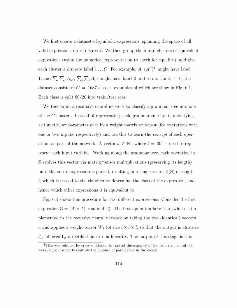
We first create a dataset of symbolic expressions, spanning the space of all

valid expressions up to degree k. We then group them into clusters of equivalent

expressions (using the numerical representation to check for equality), and give

each cluster a discrete label 1 . . . C. For example, A, (AT )T might have label

1, and∑

i

∑j Ai,j,

∑j

∑i Ai,j might have label 2 and so on. For k = 6, the

dataset consists of C = 1687 classes, examples of which are show in Fig. 6.1.

Each class is split 80/20 into train/test sets.

We then train a recursive neural network to classify a grammar tree into one

of the C clusters. Instead of representing each grammar rule by its underlying

arithmetic, we parameterize it by a weight matrix or tensor (for operations with

one or two inputs, respectively) and use this to learn the concept of each oper-

ation, as part of the network. A vector a ∈ Rl, where l = 30‡ is used to rep-

resent each input variable. Working along the grammar tree, each operation in

S evolves this vector via matrix/tensor multiplications (preserving its length)

until the entire expression is parsed, resulting in a single vector ϕ(S) of length

l, which is passed to the classifier to determine the class of the expression, and

hence which other expressions it is equivalent to.

Fig. 6.4 shows this procedure for two different expressions. Consider the first

expression S = (A. ∗ A)′ ∗ sum(A, 2). The first operation here is .∗, which is im-

plemented in the recursive neural network by taking the two (identical) vectors

a and applies a weight tensor W3 (of size l × l × l, so that the output is also size

l), followed by a rectified-linear non-linearity. The output of this stage is this‡This was selected by cross-validation to control the capacity of the recursive neural net-

work, since it directly controls the number of parameters in the model.

114

max((W3 ∗ a) ∗ a, 0). This vector is presented to the next operation, a matrix

transpose, whose output is thus max(W2 ∗ max((W3 ∗ a) ∗ a, 0), 0). Applying

the remaining operations produces a final output: ϕ(S) = max((W4 ∗ max(W2 ∗

max((W3 ∗ a) ∗ a, 0), 0)) ∗max(W1 ∗ a, 0)). This is presented to a C-way softmax

classifier to predict the class of the expression. The weights W are trained using

a cross-entropy loss and backpropagation.(((sum((sum((A * (A')), 1)), 2)) * ((A * (((sum((A'), 1)) * A)'))')) * A) ((A') * ((sum(A, 2)) * ((sum((A'), 1)) * (A * (((sum((A'), 1)) * A)')))))(sum(((sum((A * (A')), 2)) * ((sum((A'), 1)) * (A * ((A') * A)))), 1)) (sum(((A') * ((sum(A, 2)) * ((sum((A'), 1)) * (A * ((A') * A))))), 2))(((sum(A, 1)) * (((sum(A, 2)) * (sum(A, 1)))')) * (A * ((A') * A))) ((((sum(A, 2)) * ((sum((A'), 1)) * A))') * (A * (((sum((A'), 1)) * A)')))((((sum((sum((A * (A')), 1)), 2)) * ((sum((A'), 1)) * (A * ((A') * A))))')') (((sum((A'), 1)) * (A * ((A') * ((sum(A, 2)) * ((sum((A'), 1)) * A)))))')((sum(A, 1)) * (((A') * (A * ((A') * ((sum(A, 2)) * (sum(A, 1))))))')) ((((sum((A'), 1)) * A)') * ((sum((A'), 1)) * (A * (((sum((A'), 1)) * A)'))))((sum((sum((A * (A')), 1)), 2)) * ((sum((A'), 1)) * (A * ((A') * A)))) (((A * ((A') * ((sum(A, 2)) * ((sum((A'), 1)) * A))))') * (sum(A, 2)))(((sum((sum((A * (A')), 1)), 2)) * ((sum((A'), 1)) * A)) * ((A') * A)) (((A') * ((sum(A, 2)) * ((sum((A'), 1)) * A))) * (sum(((A') * A), 2)))

Class A Class B

Figure 6.1: Samples from two classes of degree k = 6 in our dataset of expressions, used to learna continuous representation of symbolic expressions via an recursive neural network. Each linerepresents a different expression, but those in the same class are equivalent to one another.

Figure 6.2: (A. ∗A)′ ∗ sum(A, 2)

.Figure 6.3: (A′. ∗A′) ∗ sum(A, 2)

.

Figure 6.4: Our recursive neural network applied to two expressions. The matrix A is representedby a fixed random vector a (of length l = 30). Each operation in the expression applies a differentmatrix (for single input operations) or tensor (for dual inputs, e.g. matrix-element multiplication)to this vector. After each operation, a rectified-linear non-linearity is applied. The weight matri-ces/tensors for each operation are shared across different expressions. The final vector is passedto a softmax classifier (not shown) to predict which class they belong to. In this example, bothexpressions are equivalent, thus should be mapped to the same class.

115

When training the recursive neural network, there are several important de-

tails that are crucial to obtaining high classification accuracy:

• The weights should be initialized to the identity, plus a small amount of

Gaussian noise added to all elements. The identity allows information to

flow the full length of the network, up to the classifier regardless of its

depth105. Without this, the recursive neural network overfits badly, pro-

ducing test accuracies of ∼ 1%.

• Rectified linear units work much better in this setting than tanh activa-

tion functions.

• We learn using a curriculum9,145, starting with the simplest expressions of

low degree and slowly increasing k.

• The weight matrix in the softmax classifier has much larger (×100) learn-

ing rate than the rest of the layers. This encourages the representation

to stay still even when targets are replaced, for example, as we move to

harder examples.

• As well as updating the weights of the recursive neural network, we also

update the initial value of a (i.e we backpropagate to the input also).

When the recursive neural network-based representation is employed for identity

discovery (see Section 6.6.3), the vector ϕ(S) is used directly (i.e. the C-way

softmax used in training is removed from the network).

116

6.5 Linear Combinations of Trees

For simple targets, an expression that matches the target may be contained

within a single grammar tree. But more complex expressions typically require

a linear combination of expressions from different trees.

To handle this, we can use the integer-based descriptors for each tree in a lin-

ear system and solve for a match to the target descriptor (if one exists). Given

a set of M trees, each with its own integer descriptor vector f , we form an M

by N linear system of equations and solve it:

Fw = t mod Zp (6.1)

where F = [f1, . . . , fM ] holds the tree representations, w is the weighting on

each of the trees and t is the target representation. The system is solved using

Gaussian elimination, where addition and multiplication is performed modulo p.

The number of solutions can vary: (a) there can be no solution, which means

that no linear combination of the current set of trees can match the target ex-

pression. If all possible trees have been enumerated, then this implies the target

expression is outside the scope of the grammar. (b) There can be one or more

solutions, meaning that some combination of the current set of trees yields a

match to the target expression.

6.6 Search Strategy

So far, we have proposed a grammar which defines the computations that are

permitted (like a programming language grammar), but it gives no guidance as

117

to how explore the space of possible expressions. Neither do the representations

we introduced help – they simply allow us to determine if an expression matches

or not. We now describe how to efficiently explore the space by learning which

paths are likely to yield a match.

Our framework uses two components: a scheduler, and a strategy. The

scheduler is fixed, and traverses space of expressions according to recommen-

dations given by the selected strategy (e.g. “Random” or “n-gram” or “recursive

neural network”). The strategy assesses which of the possible grammar rules is

likely to lead to a solution, given the current expression. Starting with the vari-

ables V (in our case a single element A, or more generally, the elements A, B

etc.), at each step the scheduler receives scores for each rule from the strategy

and picks the one with the highest score. This continues until the expression

reaches degree k and the tree is complete. We then run the linear solver to see

if a linear combination of the existing set of trees matches the target. If not,

the scheduler starts again with a new tree, initialized with the set of variables

V . The n-gram and recursive neural network strategies are learned in an incre-

mental fashion, starting with simple target expressions (i.e. those of low degree

k, such as∑

ij AAT ). Once solutions to these are found, they become train-

ing examples used to improve the strategy, needed for tackling harder targets

(e.g.∑

ij AATA).

118

6.6.1 Random Strategy

The random strategy involves no learning, thus assigns equal scores to all valid

grammar rules, hence the scheduler randomly picks which expression to try at

each step. For simple targets, this strategy may succeed as the scheduler may

stumble upon a match to the target within a reasonable time-frame. But for

complex target expressions of high degree k, the search space is huge and the

approach fails.

6.6.2 n-gram

In this strategy, we simply count how often subtrees of depth n occur in solu-

tions to previously solved targets. As the number of different subtrees of depth

n is large, the counts become very sparse as n grows. Due to this, we use a

weighted linear combination of the score from all depths up to n. We found an

effective weighting to be 10k, where k is the depth of the tree.

6.6.3 Recursive Neural Network

Section 6.4.2 showed how to use an recursive neural network to learn a contin-

uous representation of grammar trees. Recall that the recursive neural network

ϕ maps expressions to continuous vectors: ϕ(S) → Rl. To build a search strat-

egy from this, we train a softmax layer on top of the recursive neural network to

predict which rule should be applied to the current expression (or expressions,

since some rules have two inputs), so that we match the target.

Formally, we have two current branches b1 and b2 (each corresponding to an

119

expression) and wish to predict the root operation r that joins them (e.g. .∗)

from among the valid grammar rules (|r| in total). We first use the previously

trained recursive neural network to compute ϕ(b1) and ϕ(b2). These are then

presented to a |r|-way softmax layer (whose weight matrix U is of size 2l × |r|).

If only one branch exists, then b2 is set to a fixed random vector. The train-

ing data for U comes from trees that give efficient solutions to targets of lower

degree k (i.e. simpler targets). Training of the softmax layer is performed by

stochastic gradient descent. We use dropout49 as the network has a tendency to

overfit and repeat exactly the same expressions for the next value of k. Thus,

instead of training on exactly ϕ(b1) and ϕ(b2), we drop activations as we prop-

agate toward the top of the tree (the same fraction for each depth), which en-

courages the recursive neural network to capture more local structures. At test

time, the probabilities from the softmax become the scores used by the sched-

uler.

6.7 Experiments

We first show results relating to the learned representation for symbolic expres-

sions (Section 6.4.2). Then we demonstrate our framework discovering efficient

identities.

6.7.1 Expression Classification using Learned Representation

Table 6.2 shows the accuracy of the recursive neural network model on expres-

sions of varying degree, ranging from k = 3 to k = 6. The difficulty of the task

120

can be appreciated by looking at the examples in Fig. 6.1. The low error rate of

≤ 5%, despite the use of a simple softmax classifier, demonstrates the effective-

ness of our learned representation.

Degree k = 3 Degree k = 4 Degree k = 5 Degree k = 6

Test accuracy 100%± 0% 96.9%± 1.5% 94.7%± 1.0% 95.3%± 0.7%Number of classes 12 125 970 1687Number of expressions 126 1520 13038 24210

Table 6.2: Accuracy of predictions using our learned symbolic representation (averaged over 10different initializations). As the degree increases tasks becomes more challenging, because numberof classes grows, and computation trees become deeper. However our dataset grows larger too(training uses 80% of examples).

6.7.2 Efficient Identity Discovery

In our experiments we consider 5 different families of expressions, chosen to fall

within the scope of our grammar rules:

1. (∑

AAT)k: A is an Rn×n matrix. The k-th term is∑

i,j(AAT )⌊k/2⌋ for

even k

and∑

i,j(AAT )⌊k/2⌋A , for odd k. E.g. for k = 2 :

∑i,j AA

T ; for k = 3 :∑i,j AA

TA; for k = 4 :∑

i,j AATAAT etc. Naive evaluation is O(kn3).

2. (∑

(A. ∗A)AT)k: A is an Rn×n matrix and let B = A. ∗ A. The k-th

term is∑

i,j(BAT )⌊k/2⌋ for even k and∑

i,j(BATB)⌊k/2⌋ , for odd k. E.g.

for k = 2 :∑

i,j(A. ∗ A)AT ; for k = 3 :∑

i,j(A. ∗ A)AT (A. ∗ A); for

k = 4 :∑

i,j(A. ∗ A)AT (A. ∗ A)AT etc. Naive evaluation is O(kn3).

3. Symk: Elementary symmetric polynomials. A is a vector in Rn×1. For

k = 1 :∑

i Ai, for k = 2 :∑

i<j AiAj, for k = 3 :∑

i<j<k AiAjAk, etc.

121

Naive evaluation is O(nk).

4. (RBM-1)k: A is a vector in Rn×1. v is a binary n-vector. The k-th term

is:∑

v∈0,1n(vTA)k. Naive evaluation is O(2n).

5. (RBM-2)k: Taylor series terms for the partition function of an RBM.

A is a matrix in Rn×n. v and h are a binary n-vectors. The k-th term is∑v∈0,1n,h∈0,1n(v

TAh)k. Naive evaluation is O(22n).

Note that (i) for all families, the expressions yield a scalar output; (ii) the fam-

ilies are ordered in rough order of “difficulty”; (iii) we are not aware of any pre-

vious exploration of these expressions, except for Symk, which is well stud-

ied115. For the (∑

AAT)k and (∑

(A. ∗A)AT)k families we remove the matrix-

multiply rule from the grammar, thus ensuring that if any solution is found

it will be efficient since the remaining rules are at most O(kn2), rather than

O(kn3). The other families use the full grammar, given in Table 6.1. However,

the limited set of rules means that if any solution is found, it can at most be

O(n3), rather than exponential in n, as the naive evaluations would be. For

each family, we apply our framework, using the three different search strate-

gies introduced in Section 6.6. For each run we impose a fixed cut-off time of 10

minutes§ beyond which we terminate the search. At each value of k, we repeat

the experiments 10 times with different random initializations and count the

number of runs that find an efficient solution. Any non-zero count is deemed

a success, since each identity only needs to be discovered once. However, in§Running on a 3Ghz 16-core Intel Xeon. Changing the cut-off has little effect on the plots,

since the search space grows exponentially fast.

122

Fig. 6.5, we show the fraction of successful runs, which gives a sense of how

quickly the identity was found.

We start with k = 2 and increase up to k = 15, using the solutions from

previous values of k as training data for the current degree. The search space

quickly grows with k, as shown in Table 6.3. Fig. 6.5 shows results for four of

the families. We use n-grams for n = 1 . . . 5, as well as the recursive neural net-

work with two different dropout rates (0.125 and 0.3). The learning approaches

generally do much better than the random strategy for large values of k, with

the 3-gram, 4-gram and 5-gram models outperforming the recursive neural net-

work.

For the first two families, the 3-gram model reliably finds solutions. These so-

lutions involve repetition of a local patterns (e.g. Example 2), which can easily

be captured with n-gram models. However, patterns that do not have a simple

repetitive structure are much more difficult to generalize. The (RBM-2)k fam-

ily is the most challenging, involving a double exponential sum, and the solu-

tions have highly complex trees. In this case, none of our approaches performed

better than the random strategy and no solutions were discovered for k > 5.

However, the k = 5 solution was found by the recursive neural network consis-

tently faster than the random strategy (100± 12 vs 438± 77 secs).

k = 2 k = 3 k = 4 k = 5 k = 6 k = 7 and higher# Terms ≤ O

(n2)

39 171 687 2628 9785 Out of memory# Terms ≤ O(n3)

41 187 790 3197 10k+

Table 6.3: The number of possible expressions for different degrees k.

123

2 3 4 5 6 7 8 9 10 11 12 13 14 150

0.1

0.2

0.3

0.4

0.5

0.6

0.7

0.8

0.9

1

k

p(Su

cces

s)( ( AA T ) ) k

RNN0.3RNN0.13

1−gram2−gram3−gram4−gram5−gramRandom

2 3 4 5 6 7 8 9 10 11 12 13 14 150

0.1

0.2

0.3

0.4

0.5

0.6

0.7

0.8

0.9

1

k

p(Su

cces

s)

( ( A. * A ) A T ) ) k

RNN0.3RNN0.13

1−gram2−gram3−gram4−gram5−gramRandom

2 3 4 5 6 7 8 9 10 11 12 13 14 150

0.1

0.2

0.3

0.4

0.5

0.6

0.7

0.8

0.9

1

k

p(Su

cces

s)

Sym k

RNN0.3RNN0.13

1−gram2−gram3−gram4−gram5−gramRandom

2 3 4 5 6 7 8 9 10 11 12 13 14 150

0.1

0.2

0.3

0.4

0.5

0.6

0.7

0.8

0.9

1

k

p(Su

cces

s)

(RBM-1) k

RNN0.3RNN0.13

1−gram2−gram3−gram4−gram5−gramRandom

Figure 6.5: Evaluation on four different families of expressions. As the degree k increases, wesee that the random strategy consistently fails but the learning approaches can still find solutions(i.e. p(Success) is non-zero). Best viewed in electronic form.

6.7.3 Learnt solutions to (∑

AAT)k

k = 1n = 100;m = 200;A = randn(n , m) ;o r i g i na l = sum(sum(A, 1) , 2 ) ;

optimized = 1 * (sum(sum(A, 2) , 1 ) ) ;normalization = sum(abs ( o r i g i na l ( : ) ) ) ;a s se r t (sum(abs ( o r i g i na l ( : ) − optimized ( : ) ) ) / normalization < 1e−10);

k = 2n = 100;m = 200;A = randn(n , m) ;o r i g i na l = sum(sum((A * A’ ) , 1) , 2 ) ;

optimized = 1 * (sum((sum(A, 1) * A’ ) , 2 ) ) ;normalization = sum(abs ( o r i g i na l ( : ) ) ) ;a s se r t (sum(abs ( o r i g i na l ( : ) − optimized ( : ) ) ) / normalization < 1e−10);

k = 3n = 100;m = 200;A = randn(n , m) ;

124

o r i g i na l = sum(sum(( (A * A’ ) * A) , 1) , 2 ) ;

optimized = 1 * (sum((A * (sum(A, 2) ’ * A) ’ ) , 1 ) ) ;normalization = sum(abs ( o r i g i na l ( : ) ) ) ;a s se r t (sum(abs ( o r i g i na l ( : ) − optimized ( : ) ) ) / normalization < 1e−10);

k = 4n = 100;m = 200;A = randn(n , m) ;o r i g i na l = sum(sum( ( ( (A * A’ ) * A) * A’ ) , 1) , 2 ) ;

optimized = 1 * ( ( (sum(A, 1) * A’ ) * (sum(A, 1) * A’ ) ’ ) ) ;normalization = sum(abs ( o r i g i na l ( : ) ) ) ;a s se r t (sum(abs ( o r i g i na l ( : ) − optimized ( : ) ) ) / normalization < 1e−10);

k = 5n = 100;m = 200;A = randn(n , m) ;o r i g i na l = sum(sum( ( ( ( (A * A’ ) * A) * A’ ) * A) , 1) , 2 ) ;

optimized = 1 * (sum((A * ((A * (sum(A, 2) ’ * A) ’ ) ’ * A) ’ ) , 1 ) ) ;normalization = sum(abs ( o r i g i na l ( : ) ) ) ;a s se r t (sum(abs ( o r i g i na l ( : ) − optimized ( : ) ) ) / normalization < 1e−10);

6.7.4 Learnt solutions to (RBM-1)kk = 1n = 14;m = 1;A = randn (1 , n ) ;nset = dec2bin (0 : (2^(n) − 1 ) ) ;o r i g i na l = 0;fo r i = 1: s i z e ( nset , 1)

125

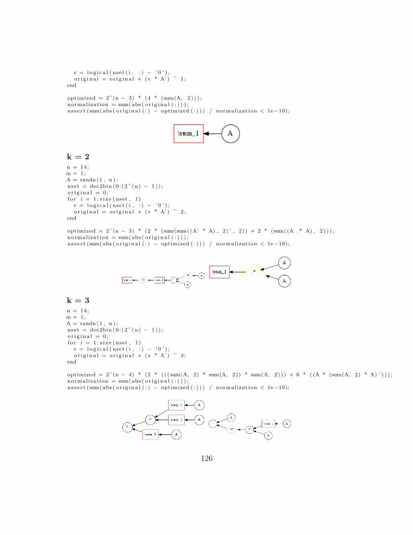
v = l o g i c a l ( nset ( i , : ) − ’ 0 ’ ) ;o r i g i na l = or i g i na l + (v * A’ ) ^ 1 ;

end

optimized = 2^(n − 3) * (4 * (sum(A, 2 ) ) ) ;normalization = sum(abs ( o r i g i na l ( : ) ) ) ;a s se r t (sum(abs ( o r i g i na l ( : ) − optimized ( : ) ) ) / normalization < 1e−10);

k = 2n = 14;m = 1;A = randn (1 , n ) ;nset = dec2bin (0 : (2^(n) − 1 ) ) ;o r i g i na l = 0;fo r i = 1: s i z e ( nset , 1)

v = l o g i c a l ( nset ( i , : ) − ’ 0 ’ ) ;o r i g i na l = or i g i na l + (v * A’ ) ^ 2 ;

end

optimized = 2^(n − 3) * (2 * (sum(sum((A’ * A) , 2) ’ , 2)) + 2 * (sum((A .* A) , 2 ) ) ) ;normalization = sum(abs ( o r i g i na l ( : ) ) ) ;a s se r t (sum(abs ( o r i g i na l ( : ) − optimized ( : ) ) ) / normalization < 1e−10);

k = 3n = 14;m = 1;A = randn (1 , n ) ;nset = dec2bin (0 : (2^(n) − 1 ) ) ;o r i g i na l = 0;fo r i = 1: s i z e ( nset , 1)

v = l o g i c a l ( nset ( i , : ) − ’ 0 ’ ) ;o r i g i na l = or i g i na l + (v * A’ ) ^ 3 ;

end

optimized = 2^(n − 4) * (2 * ( ( (sum(A, 2) * sum(A, 2)) * sum(A, 2))) + 6 * ((A * (sum(A, 2) * A) ’ ) ) ) ;normalization = sum(abs ( o r i g i na l ( : ) ) ) ;a s se r t (sum(abs ( o r i g i na l ( : ) − optimized ( : ) ) ) / normalization < 1e−10);

126

k = 4n = 14;m = 1;A = randn (1 , n ) ;nset = dec2bin (0 : (2^(n) − 1 ) ) ;o r i g i na l = 0;fo r i = 1: s i z e ( nset , 1)

v = l o g i c a l ( nset ( i , : ) − ’ 0 ’ ) ;o r i g i na l = or i g i na l + (v * A’ ) ^ 4 ;

end

optimized = 2^(n − 5) * (2 * ( ( ( ( sum(A, 2) * sum(A, 2)) * sum(A, 2)) * sum(A, 2))) +−4 * ( ( (A .* A) * (A .* A) ’ ) ) + 6 * ((A * (sum((A .* A) , 2) * A) ’ ) ) +12 * ( ( (sum(A, 2) * sum(A, 2)) * sum((A .* A) , 2 ) ) ) ) ;normalization = sum(abs ( o r i g i na l ( : ) ) ) ;a s se r t (sum(abs ( o r i g i na l ( : ) − optimized ( : ) ) ) / normalization < 1e−10);

6.7.5 Learnt solutions to (RBM-2)kk = 1n = 7;m = 8;A = randn(n , m) ;nset = dec2bin (0 : (2^(n) − 1 ) ) ;mset = dec2bin (0 : (2^(m) − 1 ) ) ;o r i g i na l = 0;fo r i = 1: s i z e ( nset , 1)

fo r j = 1: s i z e (mset , 1)v = l o g i c a l ( nset ( i , : ) − ’ 0 ’ ) ;h = l o g i c a l (mset ( j , : ) − ’ 0 ’ ) ;o r i g i na l = or i g i na l + (v * A * h ’ ) ^ 1 ;

endend

optimized = 2^(n + m − 5) * (8 * (sum(sum(A’ , 1) ’ , 1 ) ) ) ;normalization = sum(abs ( o r i g i na l ( : ) ) ) ;a s se r t (sum(abs ( o r i g i na l ( : ) − optimized ( : ) ) ) / normalization < 1e−10);

127

k = 2n = 7;m = 8;A = randn(n , m) ;nset = dec2bin (0 : (2^(n) − 1 ) ) ;mset = dec2bin (0 : (2^(m) − 1 ) ) ;o r i g i na l = 0;fo r i = 1: s i z e ( nset , 1)

fo r j = 1: s i z e (mset , 1)v = l o g i c a l ( nset ( i , : ) − ’ 0 ’ ) ;h = l o g i c a l (mset ( j , : ) − ’ 0 ’ ) ;o r i g i na l = or i g i na l + (v * A * h ’ ) ^ 2 ;

endend

optimized = 2^(n + m − 5) * (2 * (sum((sum(A, 1) .* sum(A, 1)) , 2)) +2 * (sum(sum((A .* A) , 1) , 2)) + 2 * (sum(sum((A .* repmat(sum(A, 2) , 1 , m)) , 1) ’ , 1))+ 2 * (sum((sum(A, 1) .* repmat(sum(sum(A, 1) ’ , 1) , 1 , m)) , 2 ) ) ) ;normalization = sum(abs ( o r i g i na l ( : ) ) ) ;a s se r t (sum(abs ( o r i g i na l ( : ) − optimized ( : ) ) ) / normalization < 1e−10);

k = 3n = 7;m = 8;A = randn(n , m) ;nset = dec2bin (0 : (2^(n) − 1 ) ) ;mset = dec2bin (0 : (2^(m) − 1 ) ) ;o r i g i na l = 0;fo r i = 1: s i z e ( nset , 1)

fo r j = 1: s i z e (mset , 1)v = l o g i c a l ( nset ( i , : ) − ’ 0 ’ ) ;h = l o g i c a l (mset ( j , : ) − ’ 0 ’ ) ;o r i g i na l = or i g i na l + (v * A * h ’ ) ^ 3 ;

endend

optimized = 2^(n + m − 7) * (12 * (sum(sum((A .* repmat(sum((A .* repmat(sum(A’ , 2) ’, n , 1)) , 2) , 1 , m)) , 1) , 2)) + 2 * (sum(sum((A .* repmat(sum((sum(A’ , 1) .*repmat(sum(sum(A’ , 1) ’ , 1) , 1 , n ) ) , 2) , n , m)) , 1) , 2)) + 6 * (sum(sum((A .*repmat(sum((sum(A’ , 1) .* sum(A’ , 1)) , 2) , n , m)) , 1) , 2)) + 6 * (sum(sum(( (repmat(sum(sum(A’ , 1) ’ , 1) , n , m) .* A) ’ .* A’ ) , 1) , 2)) + 6 * (sum(sum((A .*repmat(sum(( repmat(sum(sum(A’ , 1) ’ , 1) , n , m) .* A) , 1) , n , 1)) , 1) , 2 ) ) ) ;normalization = sum(abs ( o r i g i na l ( : ) ) ) ;a s se r t (sum(abs ( o r i g i na l ( : ) − optimized ( : ) ) ) / normalization < 1e−10);

128

k = 4n = 7;m = 8;A = randn(n , m) ;nset = dec2bin (0 : (2^(n) − 1 ) ) ;mset = dec2bin (0 : (2^(m) − 1 ) ) ;o r i g i na l = 0;fo r i = 1: s i z e ( nset , 1)

fo r j = 1: s i z e (mset , 1)v = l o g i c a l ( nset ( i , : ) − ’ 0 ’ ) ;h = l o g i c a l (mset ( j , : ) − ’ 0 ’ ) ;o r i g i na l = or i g i na l + (v * A * h ’ ) ^ 4 ;

endend

optimized = 2^(n + m − 9) * (24 * ((sum(A, 1) * sum(( repmat(sum((repmat(sum(A, 1) , n , 1) .* A) ’ , 1) , m, 1) .* A’ ) , 2)) ) + 6 * (sum(sum((A .*repmat(sum((A .* repmat(sum((sum(A’ , 1) .* sum(A’ , 1)) , 2) , n , m)) , 2) , 1 , m)) , 1) ,2)) + −24 * (sum(sum((A .* repmat(sum((A .* repmat(sum((A .* A) , 1) , n , 1)) , 1) ,n , 1)) , 1) , 2)) + 8 * (sum(sum(( (A’ ’ .* (A .* A)) .* A) , 1) , 2)) + 12 *(sum(sum((A .* repmat(sum((A .* repmat(sum(sum((A .* A) , 1) , 2) , n , m)) , 2) , 1 , m)) ,1) , 2)) + −24 * (sum(sum((A .* repmat(sum((A .* repmat(sum((A .* A) , 2) , 1 , m)) ,

2) , 1 , m)) , 1) , 2)) + 12 * (sum(sum(( (A * A’ ) .* (A * A’ ) ) , 1) , 2)) + 12 *(sum(sum((A .* repmat(sum((A .* repmat(sum((sum(A, 1) .* repmat(sum(sum(A, 1) ’ , 1) , 1 , m)) , 2) , n , m)) , 2) , 1 , m)) , 1) , 2)) + −4 * (sum(sum((A .*repmat(sum(( repmat(sum(A, 1) , n , 1) .* ( repmat(sum(A, 1) , n , 1) .* A)) , 1) , n , 1)) ,1) , 2)) + 24 * (sum(sum((A .* repmat(sum((A .* repmat(sum((A .*repmat(sum(A, 2) , 1 , m)) , 1) , n , 1)) , 2) , 1 , m)) , 1) , 2)) + 2 * (sum(sum((A .*repmat(sum(sum((A .* repmat(sum((sum(A, 1) .* repmat(sum(sum(A, 1) ’ , 1) , 1 , m)) ,2) , n , m)) , 1) , 2) , n , m)) , 1) , 2)) + 12 * (sum(( repmat(sum(sum(A, 1) , 2) , 1 , m).* ( repmat(sum(sum(A, 1) ’ , 1) , 1 , m) .* sum((A .* A) , 1 ) ) ) , 2)) + 12 * (sum(sum((A .* repmat(sum((A .* repmat(sum(sum((A .* A) , 1) , 2) , n , m)) , 1) , n , 1)) , 1) , 2))+ 6 * (sum(sum((A .* repmat(sum((A .* repmat(sum((sum(A, 1) .* sum(A, 1)) , 2) , n , m)), 1) , n , 1)) , 1) , 2)) + 6 * (sum((sum((A .* A) , 2) .* repmat(sum(sum((A .* A) , 1) , 2) , n , 1)) , 1)) + 12 * (sum(sum((A .* repmat(sum((A .* repmat(sum((sum(A, 1) .* sum(A, 1)), 2) , n , m)) , 2) , 1 , m)) , 1) , 2)) + 48 * (sum(sum((A .* repmat(sum(sum((A .*repmat(sum((A .* repmat(sum(A, 2) , 1 , m)) , 1) , n , 1)) , 1) , 2) , n , m)) , 1) , 2))+ −12 * (sum((sum((A .* A) , 2) .* sum((A .* A) , 2)) , 1)) + −12 * (sum((sum((A .*

A) , 1) .* sum((A .* A) , 1)) , 2)) + 12 * (sum(sum((A .* repmat(sum(sum((A .*repmat(sum((sum(A, 1) .* sum(A, 1)) , 2) , n , m)) , 1) , 2) , n , m)) , 1) , 2)) + −4* (sum(sum((A .* repmat(sum((A .* repmat(sum((A .* repmat(sum(A, 2) , 1 , m)) , 2) ,1 , m)) , 2) , 1 , m)) , 1) , 2 ) ) ) ;normalization = sum(abs ( o r i g i na l ( : ) ) ) ;a s se r t (sum(abs ( o r i g i na l ( : ) − optimized ( : ) ) ) / normalization < 1e−10);

129

6.8 Discussion

We have introduced a framework based on a grammar of symbolic operations

for discovering mathematical identities. Through the novel application of learn-

ing methods, we have shown how the exploration of the search space can be

learned from previously successful solutions to simpler expressions. This allows

us to discover complex expressions that random or brute-force strategies cannot

find.

Some of the families considered in this paper are close to expressions often en-

countered in machine learning. For example, dropout involves an exponential

sum over binary masks, which is related to the RBM-1 family. Also, the par-

tition function of an RBM can be approximated by the RBM-2 family. Hence

130

the identities we have discovered could potentially be used to give a closed-form

version of dropout, or compute the RBM partition function efficiently (i.e. in

polynomial time). Additionally, the automatic nature of our system naturally

lends itself to integration with compilers, or other optimization tools, where it

could replace computations with efficient versions thereof.

The problem addressed in this paper involves discrete over programs, which

due to Solomonoff induction is a core program with AI. Our successful use of

machine learning to guide the search gives hope that similar techniques might

be effective over broader domain than mathematical expressions across matrices.

131

7Conclusions

7.1 Summary of Contributions

This thesis is concerned with the problem of learning algorithms from data, as

we consider this task to be pivotal in the area of artificial intelligence. We have

made several contributions in this direction:

• Measured to what extent modern neural networks can learn algorithms

like copying, adding numbers, and interpreting Python code (Chapter 3);

• Formulated a new curriculum learning strategy that substantially im-

proves generalization (Chapter 3);

132

• Introduced discrete interfaces and methods to train neural networks with

such interfaces, based on REINFORCE and Q-learning (Chapter 4);

• Proposed several enhancements to Q-learning such as dynamic discount

and penalty on the Q-function (Chapter 4);

• Invented a gradient verification technique for REINFORCE (Chapter 4);

• Created one of the very few statistical models that is theoretically Turing

complete (Chapter 4). However, empirically our model cannot solve any

task that would require Turing completeness;

• Showed how to rediscover the convolution algorithm from data (Chap-

ter 5);

• Described a connection between convolution and harmonic analysis on

graphs (Chapter 5);

• Created a novel grammar framework for finding efficient versions of sym-

bolic expressions (Chapter 6);

• Integrated machine learning techniques to learn a prior that guides the

search over symbolic expressions (Chapter 6);

• Learned a continuous representation of mathematical structures using re-

cursive neural networks, making the symbolic domain accessible to many

other learning approaches (Chapter 6); and

133

• Discovered many new mathematical identities which offer significant re-

ductions in the computational complexity of certain expressions (Chap-

ter 6).

Chapter 3 shows that it’s easy to deceive ourselves that neural networks are

already able to learn concepts with small Kolmogorov complexities. Lack of gen-

eralization is a signal that tells us when this is not happening The rise of the

Big Data paradigm only makes it easier to falsely conclude that our models un-

derstand data due to the their increased ability to memorize it.

In Chapter 4, we propose a way to encourage neural networks to find solu-

tions with small Kolmogorov complexities by augmenting them with interfaces.

Interfaces allow us to express some concepts in more concise ways, and encour-

age the model to find a solution with small Kolmogorov complexity. This ap-

proach frequently results in solutions that generalize to the entire data distribu-

tion. However, sometimes a solution fails to generalize. In such cases, the model

has not learned an underlying algorithm. Such breakdowns can occur even in

the simplest possible learning scenarios, in which all actions over the interfaces

are supervised. We have shown that the difficulty arises in expressing an algo-

rithm using a neural network, rather than from the search induced by reinforce-

ment learning.

Chapter 5 takes a route opposite to the one taken by Chapter 4. Instead of

learning algorithms that are above the reach of the contemporary techniques, we

investigate whether we can automatically rediscover currently used methods. In

particular, we aim to rediscover the convolution neural network. We achieve this

134

goal by abstracting concepts like grid, locality, and multi-resolution.

Finally, in Chapter 6, we propose a method to find automatically fast im-

plementations for mathematical formulas in linear algebra. We directly search

over a set of constrained short programs. Such a procedure is encouraged by

Solomonoff induction. However, the number of programs to explore grows ex-

ponentially in their length, rendering the search computationally infeasible. To

make this search tractable, we guide it with a prior given by n-grams and a neu-

ral network. We were able to automatically find several mathematical formulas

that were hitherto unknown.

7.2 Future Directions

We believe that a sound machine learning system of the future must internally

encode various algorithms. Here, we propose several speculative directions to

achieve this goal:

• Transfer Learning97, Lifetime Learning125, Curriculum Learn-

ing9. All these concepts account for training a model on tasks that have

an increasing complexity88. The model has to transfer its knowledge from

a simple task to a hard one. For example, children learn mathematics

gradually, first beginning with arithmetic and geometry. Only after mas-

tering these topics do they move on to more advanced ones, such as differ-

ential calculus. How should we modify our models and train algorithms in

order to achieve transfer learning in an analogous manner?

135

• Learning optimization procedures. There are many optimization

techniques, such as SGD, Adam63, Hessian-Free83, k-fac84 etc. Optimiza-

tion is an example of an algorithm. We ask whether it is possible to learn

the core structure of optimization itself.

• Permanent, unbounded storage. Several recent models provide ways

of using external memory41,136,42,57,2. This type of memory can assume

various topologies: it can be accessible as a stack57, a hash table41, or a

hierarchical hash table2. So far, external memory has been used as ephemeral

storage, whose lifetime only spans the computation necessary to process a

single sample. In other words, the memory is reset between samples. The

weights of a neural network provide a method for permanent storage, but

they have a fixed topology. Would it be possible to store neural network

weights in permanent memory and access them on demand. This type of

storage could encourage algorithm sharing.

Many of ideas above are tempting to work on, and it is hard to settle on one

of them. Andrew Ng (personal communication, summer 2015) suggested making

a choice based on the potential future impact of an idea, and I will follow this

advice when choosing what to work on next.

136

References

[1] Aberdeen, D. & Baxter, J. (2002). Scaling internal-state policy-gradient

methods for pomdps. In Proceedings of the Nineteenth International Con-

ference on Machine Learning (ICML 2002) (pp. 3–10).

[2] Andrychowicz, M. & Kurach, K. (2016). Learning efficient algorithms with

hierarchical attentive memory. arXiv preprint arXiv:1602.03218.

[3] Ba, J., Mnih, V., & Kavukcuoglu, K. (2014). Multiple object recognition

with visual attention. arXiv preprint arXiv:1412.7755.

[4] Bahdanau, D., Cho, K., & Bengio, Y. (2014a). Neural machine translation

by jointly learning to align and translate. arXiv preprint arXiv:1409.0473.

[5] Bahdanau, D., Cho, K., & Bengio, Y. (2014b). Neural machine translation

by jointly learning to align and translate. arXiv preprint arXiv:1409.0473.

[6] Belkin, M. & Niyogi, P. (2001). Laplacian eigenmaps and spectral tech-

niques for embedding and clustering. In NIPS, volume 14 (pp. 585–591).

[7] Bengio, Y., Frasconi, P., & Simard, P. (1993). The problem of learning

long-term dependencies in recurrent networks. In Neural Networks, 1993.,

IEEE International Conference on (pp. 1183–1188).: IEEE.

137

[8] Bengio, Y., Louradour, J., Collobert, R., & Weston, J. (2009a). Curricu-

lum learning. In Proceedings of the 26th annual international conference

on machine learning (pp. 41–48).: ACM.

[9] Bengio, Y., Louradour, J., Collobert, R., & Weston, J. (2009b). Curricu-

lum learning. In ICML.

[10] Bengio, Y., Simard, P., & Frasconi, P. (1994). Learning long-term depen-

dencies with gradient descent is difficult. Neural Networks, IEEE Transac-

tions on, 5(2), 157–166.

[11] Bishop, C. M. (2006). Pattern recognition. Machine Learning.

[12] Bowman, S. R. (2013). Can recursive neural tensor networks learn logical

reasoning? arXiv preprint arXiv:1312.6192.

[13] Box, G. E. & Tiao, G. C. (2011). Bayesian inference in statistical analy-

sis, volume 40. John Wiley & Sons.

[14] Brooks, S. P. & Morgan, B. J. (1995). Optimization using simulated an-

nealing. The Statistician, (pp. 241–257).

[15] Bruna, J., Zaremba, W., Szlam, A., & LeCun, Y. (2013). Spectral

networks and locally connected networks on graphs. arXiv preprint

arXiv:1312.6203.

[16] Chan, P. K. & Stolfo, S. J. (1993). Experiments on multistrategy learning

by meta-learning. In Proceedings of the second international conference on

information and knowledge management (pp. 314–323).: ACM.

138

[17] Cheung, G. & McCanne, S. (1999). An attribute grammar based frame-

work for machine-dependent computational optimization of media process-

ing algorithms. In ICIP, volume 2 (pp. 797–801).: IEEE.

[18] Cho, K., van Merriënboer, B., Bahdanau, D., & Bengio, Y. (2014). On

the properties of neural machine translation: Encoder-decoder approaches.

arXiv preprint arXiv:1409.1259.

[Chung] Chung, F. R. K. Spectral Graph Theory. American Mathematical Soci-

ety.

[20] Coates, A. & Ng, A. Y. (2011). Selecting receptive fields in deep networks.

In Advances in Neural Information Processing Systems.

[21] Coifman, R. & Maggioni, M. (2006). Diffusion wavelets. Appl. Comp.

Harm. Anal., 21(1), 53–94.

[22] Collobert, R. & Weston, J. (2008). A unified architecture for natural lan-

guage processing: deep neural networks with multitask learning. In ICML.

[23] Crovella, M. & Kolaczyk, E. D. (2003). Graph wavelets for spatial traffic

analysis. In INFOCOM.

[24] Cybenko, G. (1989). Approximation by superpositions of a sigmoidal func-

tion. Mathematics of control, signals and systems, 2(4), 303–314.

[25] Das, S., Giles, C. L., & Sun, G.-Z. (1992). Learning context-free gram-

mars: Capabilities and limitations of a recurrent neural network with an

139

external stack memory. In In Proceedings of The Fourteenth Annual Con-

ference of Cognitive Science Society.

[26] Daumé Iii, H., Langford, J., & Marcu, D. (2009). Search-based structured

prediction. Machine learning, 75(3), 297–325.

[27] Davies, W. & Edwards, P. (2000). Dagger: A new approach to combining

multiple models learned from disjoint subsets. machine Learning, 2000,

1–16.

[28] Dennis Jr, J. E. & Schnabel, R. B. (1996). Numerical methods for uncon-

strained optimization and nonlinear equations, volume 16. Siam.

[29] Desainte-Catherine, M. & Barbar, K. (1994). Using attribute grammars to

find solutions for musical equational programs. ACM SIGPLAN Notices,

29(9), 56–63.

[30] Dhillon, I. S., Guan, Y., & Kulis, B. (2007). Weighted graph cuts without

eigenvectors a multilevel approach. IEEE Trans. Pattern Anal. Mach.

Intell., 29(11), 1944–1957.

[31] Dietterich, T. G., Domingos, P., Getoor, L., Muggleton, S., & Tadepalli,

P. (2008). Structured machine learning: the next ten years. Machine

Learning, 73(1), 3–23.

[32] Einstein, A. (1916). The foundation of the generalised theory of relativ-

ity. On a Heuristic Point of View about the Creation and Conversion of

Light 1 On the Electrodynamics of Moving Bodies 10 The Development

140

of Our Views on the Composition and Essence of Radiation 11 The Field

Equations of Gravitation 19 The Foundation of the Generalised Theory of

Relativity 22, (pp.22).

[33] Einstein, A. & Press, A. (2005). What is the Theory of Relativity?

Springer.

[34] Gauch, H. G. (2003). Scientific method in practice. Cambridge University

Press.

[35] Gavish, M., Nadler, B., & Coifman, R. R. (2010). Multiscale wavelets on

trees, graphs and high dimensional data: Theory and applications to semi

supervised learning. In J. Frankranz & T. Joachims (Eds.), ICML (pp.

367–374).

[36] Glorot, X. & Bengio, Y. (2010). Understanding the difficulty of training

deep feedforward neural networks. In International conference on artificial

intelligence and statistics (pp. 249–256).

[37] Goodman, N., Mansinghka, V., Roy, D., Bonawitz, K., & Tarlow, D.

(2012). Church: a language for generative models. arXiv:1206.3255.

[38] Graves, A. (2013). Generating sequences with recurrent neural networks.

arXiv preprint arXiv:1308.0850.

[39] Graves, A., Mohamed, A.-r., & Hinton, G. (2013). Speech recognition

with deep recurrent neural networks. In Acoustics, Speech and Signal Pro-

141

cessing (ICASSP), 2013 IEEE International Conference on (pp. 6645–

6649).: IEEE.

[40] Graves, A. & Schmidhuber, J. (2005). Framewise phoneme classification

with bidirectional lstm and other neural network architectures. Neural

Networks, 18(5), 602–610.

[41] Graves, A., Wayne, G., & Danihelka, I. (2014). Neural turing machines.

arXiv preprint arXiv:1410.5401.

[42] Grefenstette, E., Hermann, K. M., Suleyman, M., & Blunsom, P. (2015).

Learning to transduce with unbounded memory. arXiv preprint

arXiv:1506.02516.

[43] Gregor, K. & LeCun, Y. (2010). Emergence of complex-like cells in a tem-

poral product network with local receptive fields. CoRR, abs/1006.0448.

[44] Guskov, I., Sweldens, W., & Schröder, P. (1999). Multiresolution signal

processing for meshes. Computer Graphics Proceedings (SIGGRAPH 99),

(pp. 325–334).

[45] Hastie, T., Tibshirani, R., & Friedman, J. (2009). The elements of statisti-

cal learning: data mining, inference and prediction. Springer, 2 edition.

[46] Hill, T. P. (1995). A statistical derivation of the significant-digit law. Sta-

tistical Science, (pp. 354–363).

[47] Hinton, G., Deng, L., Yu, D., Dahl, G. E., Mohamed, A.-r., Jaitly, N., Se-

nior, A., Vanhoucke, V., Nguyen, P., Sainath, T. N., et al. (2012a). Deep

142

neural networks for acoustic modeling in speech recognition: The shared

views of four research groups. Signal Processing Magazine, IEEE, 29(6),

82–97.

[48] Hinton, G. E., Deng, L., Yu, D., Dahl, G. E., rahman Mohamed, A.,

Jaitly, N., Senior, A., Vanhoucke, V., Nguyen, P., Sainath, T. N., &

Kingsbury, B. (2012b). Deep neural networks for acoustic modeling in

speech recognition: The shared views of four research groups. IEEE Signal

Process. Mag., 29(6), 82–97.

[49] Hinton, G. E., Srivastava, N., Krizhevsky, A., Sutskever, I., & Salakhut-

dinov, R. R. (2012c). Improving neural networks by preventing co-

adaptation of feature detectors. arXiv:1207.0580.

[50] Hochreiter, S. (1991). Untersuchungen zu dynamischen neuronalen netzen.

Master’s thesis, Institut fur Informatik, Technische Universitat, Munchen.

[51] Hochreiter, S. & Schmidhuber, J. (1997). Long short-term memory. Neural

computation, 9(8), 1735–1780.

[52] Hoffmann, R., Minkin, V. I., & Carpenter, B. K. (1996). Ockham’s razor

and chemistry. Bulletin de la Société chimique de France, 133(2), 117–130.

[53] Howard, A. G. (2013). Some improvements on deep convolutional neural

network based image classification. arXiv preprint arXiv:1312.5402.

143

[54] Ioffe, S. & Szegedy, C. (2015). Batch normalization: Accelerating deep

network training by reducing internal covariate shift. arXiv preprint

arXiv:1502.03167.

[55] Jacobs, A. (2009). The pathologies of big data. Communications of the

ACM, 52(8), 36–44.

[56] Joachims, T., Finley, T., & Yu, C.-N. J. (2009). Cutting-plane training of

structural svms. Machine Learning, 77(1), 27–59.

[57] Joulin, A. & Mikolov, T. (2015). Inferring algorithmic patterns with stack-

augmented recurrent nets. arXiv preprint arXiv:1503.01007.

[58] Jozefowicz, R., Vinyals, O., Schuster, M., Shazeer, N., & Wu, Y.

(2016). Exploring the limits of language modeling. arXiv preprint

arXiv:1602.02410.

[59] Jozefowicz, R., Zaremba, W., & Sutskever, I. (2015). An empirical explo-

ration of recurrent network architectures. In Proceedings of the 32nd In-

ternational Conference on Machine Learning (ICML-15) (pp. 2342–2350).

[60] Kaiser, Ł. & Sutskever, I. (2015). Neural gpus learn algorithms. arXiv

preprint arXiv:1511.08228.

[61] Kalchbrenner, N. & Blunsom, P. (2013). Recurrent continuous translation

models. In EMNLP.

[62] Karypis, G. & Kumar, V. (1995). METIS - Unstructured Graph Partition-

ing and Sparse Matrix Ordering System, Version 2.0. Technical report.

144

[63] Kingma, D. & Ba, J. (2014). Adam: A method for stochastic optimiza-

tion. arXiv preprint arXiv:1412.6980.

[64] Knuth, D. E. (1968). Semantics of context-free languages. Mathematical

systems theory, 2(2), 127–145.

[65] Kohl, N. & Stone, P. (2004). Policy gradient reinforcement learning for

fast quadrupedal locomotion. In Robotics and Automation, 2004. Proceed-

ings. ICRA’04. 2004 IEEE International Conference on, volume 3 (pp.

2619–2624).: IEEE.

[66] Kouvelis, P. & Yu, G. (2013). Robust discrete optimization and its appli-

cations, volume 14. Springer Science & Business Media.

[67] Krizhevsky, A., Sutskever, I., & Hinton, G. (2012). Imagenet classification

with deep convolutional neural networks. In Advances in Neural Informa-

tion Processing Systems 25 (pp. 1106–1114).

[68] Kurach, K., Andrychowicz, M., & Sutskever, I. (2015). Neural random-

access machines. arXiv preprint arXiv:1511.06392.

[69] Kushnir, D., Galun, M., & Brandt, A. (2006). Fast multiscale clustering

and manifold identification. Pattern Recognition, 39(10), 1876 – 1891.

<ce:title>Similarity-based Pattern Recognition</ce:title>.

[70] Kushnir, D., Galun, M., & Brandt, A. (2010). Efficient multilevel eigen-

solvers with applications to data analysis tasks. Pattern Analysis and

Machine Intelligence, IEEE Transactions on, 32(8), 1377–1391.

145

[71] Le, Q. V., Jaitly, N., & Hinton, G. E. (2015). A simple way to ini-

tialize recurrent networks of rectified linear units. arXiv preprint

arXiv:1504.00941.

[72] Le, Q. V., Ngiam, J., Chen, Z., Chia, D., Koh, P. W., & Ng, A. Y. (2010).

Tiled convolutional neural networks. In In NIPS.

[73] Le, Q. V., Zou, W. Y., Yeung, S. Y., & Ng, A. Y. (2011). Learning hierar-

chical invariant spatio-temporal features for action recognition with inde-

pendent subspace analysis. In Computer Vision and Pattern Recognition

(CVPR), 2011 IEEE Conference on (pp. 3361–3368).: IEEE.

[74] Le Roux, N., Bengio, Y., Lamblin, P., Joliveau, M., Kégl, B., et al. (2007).

Learning the 2-d topology of images. In NIPS.

[75] LeCun, Y. & Bengio, Y. (1995). Convolutional networks for images,

speech, and time series. The handbook of brain theory and neural net-

works, 3361(10), 1995.

[76] LeCun, Y., Bottou, L., Bengio, Y., & Haffner, P. (2001). Gradient-based

learning applied to document recognition. In Intelligent Signal Processing

(pp. 306–351).: IEEE Press.

[77] Levin, L. A. (1984). Randomness conservation inequalities; information

and independence in mathematical theories. Information and Control,

61(1), 15–37.

146

[78] Li, M. & Vitányi, P. (2013). An introduction to Kolmogorov complexity

and its applications. Springer Science & Business Media.

[79] Liang, P., Jordan, M. I., & Klein, D. (2013). Learning dependency-based

compositional semantics. Computational Linguistics, 39(2), 389–446.

[80] Lohr, S. (2012). The age of big data. New York Times, 11.

[81] Luong, M.-T., Sutskever, I., Le, Q. V., Vinyals, O., & Zaremba, W.

(2014). Addressing the rare word problem in neural machine translation.

arXiv preprint arXiv:1410.8206.

[82] Mao, J., Xu, W., Yang, Y., Wang, J., Huang, Z., & Yuille, A. (2014).

Deep captioning with multimodal recurrent neural networks (m-rnn).

arXiv preprint arXiv:1412.6632.

[83] Martens, J. (2010). Deep learning via hessian-free optimization. In

Proceedings of the 27th International Conference on Machine Learning

(ICML-10) (pp. 735–742).

[84] Martens, J. & Grosse, R. (2015). Optimizing neural networks

with kronecker-factored approximate curvature. arXiv preprint

arXiv:1503.05671.

[85] Martens, J. & Sutskever, I. (2011). Learning recurrent neural networks

with hessian-free optimization. In Proceedings of the 28th International

Conference on Machine Learning (ICML-11) (pp. 1033–1040).

147

[86] Mikolov, T. (2012). Statistical language models based on neural networks.

PhD thesis, Ph. D. thesis, Brno University of Technology.

[87] Mikolov, T., Chen, K., Corrado, G., & Dean, J. (2013). Efficient estima-

tion of word representations in vector space. arXiv:1301.3781.

[88] Mikolov, T., Joulin, A., & Baroni, M. (2015). A roadmap towards machine

intelligence. arXiv preprint arXiv:1511.08130.

[89] Mikolov, T., Joulin, A., Chopra, S., Mathieu, M., & Ranzato, M. (2014).

Learning longer memory in recurrent neural networks. arXiv preprint

arXiv:1412.7753.

[90] Mikolov, T., Karafiát, M., Burget, L., Cernockỳ, J., & Khudanpur, S.

(2010). Recurrent neural network based language model. In INTER-

SPEECH (pp. 1045–1048).

[91] Minsky, M. & Papert, S. (1969). Perceptrons.

[92] Mitchell, M. (1998). An introduction to genetic algorithms. MIT press.

[93] Mnih, V., Heess, N., Graves, A., et al. (2014). Recurrent models of visual

attention. In Advances in Neural Information Processing Systems (pp.

2204–2212).

[94] Mohamed, A.-r., Dahl, G. E., & Hinton, G. (2012). Acoustic modeling

using deep belief networks. Audio, Speech, and Language Processing, IEEE

Transactions on, 20(1), 14–22.

148

[95] Nordin, P. (1997). Evolutionary program induction of binary machine code

and its applications. Krehl Munster.

[96] O’Neill, M., Cleary, R., & Nikolov, N. (2004). Solving knapsack problems

with attribute grammars. In Proceedings of the Third Grammatical Evolu-

tion Workshop (GEWS’04): Citeseer.

[97] Pan, S. J. & Yang, Q. (2010). A survey on transfer learning. Knowledge

and Data Engineering, IEEE Transactions on, 22(10), 1345–1359.

[98] Peters, J. & Schaal, S. (2006). Policy gradient methods for robotics. In

Intelligent Robots and Systems, 2006 IEEE/RSJ International Conference

on (pp. 2219–2225).: IEEE.

[99] Pfeffer, A. (2011). Practical probabilistic programming. In Inductive Logic

Programming (pp. 2–3). Springer.

[100] Ranzato, M., Chopra, S., Auli, M., & Zaremba, W. (2015). Sequence level

training with recurrent neural networks. arXiv preprint arXiv:1511.06732.

[101] Rissanen, J. (1983). A universal prior for integers and estimation by mini-

mum description length. The Annals of statistics, (pp. 416–431).

[102] Rubinstein, R. Y. & Kroese, D. P. (2013). The cross-entropy method: a

unified approach to combinatorial optimization, Monte-Carlo simulation

and machine learning. Springer Science & Business Media.

[103] Rustamov, R. M. & Guibas, L. (2013). Wavelets on graphs via deep learn-

ing. In NIPS.

149

[104] Ruzzo, W. L. (1981). On uniform circuit complexity. Journal of Computer

and System Sciences, 22(3), 365–383.

[105] Saxe, A. M., McClelland, J. L., & Ganguli, S. (2013). Exact solutions

to the nonlinear dynamics of learning in deep linear neural networks.

arXiv:1312.6120.

[106] Schmidhuber, J. (2004). Optimal ordered problem solver. Machine Learn-

ing, 54(3), 211–254.

[107] Schmidhuber, J. (2012). Self-delimiting neural networks. arXiv preprint

arXiv:1210.0118.

[108] Sermanet, P., Chintala, S., & LeCun, Y. (2012). Convolutional neural

networks applied to house numbers digit classification. In International

Conference on Pattern Recognition (ICPR 2012).

[109] Sermanet, P., Eigen, D., Zhang, X., Mathieu, M., Fergus, R., & LeCun, Y.

(2013). Overfeat: Integrated recognition, localization and detection using

convolutional networks. arXiv preprint arXiv:1312.6229.

[110] Simon, P. (2013). Too Big to Ignore: The Business Case for Big Data,

volume 72. John Wiley & Sons.

[111] Sipser, M. (1983). Borel sets and circuit complexity. In Proceedings of the

fifteenth annual ACM symposium on Theory of computing (pp. 61–69).:

ACM.

150

[112] Smolensky, R. (1987). Algebraic methods in the theory of lower bounds

for boolean circuit complexity. In Proceedings of the nineteenth annual

ACM symposium on Theory of computing (pp. 77–82).: ACM.

[113] Socher, R., Perelygin, A., Wu, J. Y., Chuang, J., Manning, C. D., Ng,

A. Y., & Potts, C. P. (2013). Recursive deep models for semantic com-

positionality over a sentiment treebank. In EMNLP.

[114] Solomonoff, R. J. (1964). A formal theory of inductive inference. Part I.

Information and control, 7(1), 1–22.

[115] Stanley, R. P. (2011). Enumerative combinatorics. Number 49. Cambridge

university press.

[116] Sukhbaatar, S., Szlam, A., Weston, J., & Fergus, R. (2015). Weakly super-

vised memory networks. arXiv preprint arXiv:1503.08895.

[117] Sutskever, I., Martens, J., & Hinton, G. E. (2011). Generating text with

recurrent neural networks. In Proceedings of the 28th International Con-

ference on Machine Learning (ICML-11) (pp. 1017–1024).

[118] Sutskever, I., Vinyals, O., & Le, Q. V. (2014). Sequence to sequence learn-

ing with neural networks. In Advances in neural information processing

systems (pp. 3104–3112).

[119] Sutton, R. S. (1990). Integrated architectures for learning, planning, and

reacting based on approximating dynamic programming. In Proceedings of

the seventh international conference on machine learning (pp. 216–224).

151

[120] Sutton, R. S. & Barto, A. G. (1998). Reinforcement learning: An intro-

duction, volume 1. MIT press Cambridge.

[121] Szegedy, C., Ioffe, S., & Vanhoucke, V. (2016). Inception-v4, inception-

resnet and the impact of residual connections on learning. arXiv preprint

arXiv:1602.07261.

[122] Szegedy, C., Liu, W., Jia, Y., Sermanet, P., Reed, S., Anguelov, D., Er-

han, D., Vanhoucke, V., & Rabinovich, A. (2015). Going deeper with con-

volutions. In Proceedings of the IEEE Conference on Computer Vision

and Pattern Recognition (pp. 1–9).

[123] Taskar, B., Chatalbashev, V., Koller, D., & Guestrin, C. (2005). Learning

structured prediction models: A large margin approach. In Proceedings

of the 22nd international conference on Machine learning (pp. 896–903).:

ACM.

[124] Taylor, G., Fergus, R., LeCun, Y., & Bregler, C. (2010). Convolutional

learning of spatio-temporal features. In Proc. European Conference on

Computer Vision (ECCV’10).

[125] Thrun, S. & Pratt, L. (2012). Learning to learn. Springer Science & Busi-

ness Media.

[126] Trottenberg, U. & Schuller, A. (2001). Multigrid. Orlando, FL, USA:

Academic Press, Inc.

[127] Vapnik, V. (1998). Statistical learning theory, volume 1. Wiley New York.

152

[128] Vilalta, R. & Drissi, Y. (2002). A perspective view and survey of meta-

learning. Artificial Intelligence Review, 18(2), 77–95.

[129] Vinyals, O., Toshev, A., Bengio, S., & Erhan, D. (2015). Show and tell: A

neural image caption generator. In Proceedings of the IEEE Conference on

Computer Vision and Pattern Recognition (pp. 3156–3164).

[130] Vitányi, P. & Li, M. (2000). Minimum description length induction,

bayesianism, and kolmogorov complexity. Information Theory, IEEE

Transactions on, 46(2), 446–464.

[131] von Luxburg, U. (2006). A tutorial on spectral clustering. Technical Re-

port 149.

[132] Waldispühl, J., Behzadi, B., & Steyaert, J.-M. (2002). An approximate

matching algorithm for finding (sub-) optimal sequences in s-attributed

grammars. Bioinformatics, 18(suppl 2), S250–S259.

[133] Watkins, C. (1989). Learning from Delayed Rewards. PhD thesis, Cam-

brdige University.

[134] Watkins, C. J. & Dayan, P. (1992). Q-learning. Machine learning, 8(3-4),

279–292.

[135] Wegener, I. et al. (1987). The complexity of Boolean functions, volume 1.

BG Teubner Stuttgart.

[136] Weston, J., Chopra, S., & Bordes, A. (2014). Memory networks. arXiv

preprint arXiv:1410.3916.

153

[137] Wilamowski, B. M., Hunter, D., & Malinowski, A. (2003). Solving parity-

n problems with feedforward neural networks. In Neural Networks, 2003.

Proceedings of the International Joint Conference on, volume 4 (pp. 2546–

2551).: IEEE.

[138] Williams, R. J. (1992a). Simple statistical gradient-following algorithms

for connectionist reinforcement learning. Machine learning, 8(3-4), 229–

256.

[139] Williams, R. J. (1992b). Simple statistical gradient-following algorithms

for connectionist reinforcement learning. Machine learning, 8(3-4), 229–

256.

[140] Wineberg, M. & Oppacher, F. (1994). A representation scheme to perform

program induction in a canonical genetic algorithm. In Parallel Problem

Solving from Nature—PPSN III (pp. 291–301). Springer.

[141] Wu, X., Zhu, X., Wu, G.-Q., & Ding, W. (2014). Data mining with big

data. Knowledge and Data Engineering, IEEE Transactions on, 26(1),

97–107.

[142] Xu, K., Ba, J., Kiros, R., Courville, A., Salakhutdinov, R., Zemel, R., &

Bengio, Y. (2015). Show, attend and tell: Neural image caption generation

with visual attention. arXiv preprint arXiv:1502.03044.

154

[143] Zaremba, W., Kurach, K., & Fergus, R. (2014a). Learning to discover

efficient mathematical identities. In Advances in Neural Information Pro-

cessing Systems (pp. 1278–1286).

[144] Zaremba, W., Mikolov, T., Joulin, A., & Fergus, R. (2015). Learning sim-

ple algorithms from examples. arXiv preprint arXiv:1511.07275.

[145] Zaremba, W. & Sutskever, I. (2014). Learning to execute. arXiv preprint

arXiv:1410.4615.

[146] Zaremba, W. & Sutskever, I. (2015). Reinforcement learning neural turing

machines. arXiv preprint arXiv:1505.00521.

[147] Zaremba, W., Sutskever, I., & Vinyals, O. (2014b). Recurrent neural net-

work regularization. arXiv preprint arXiv:1409.2329.

155