learning ancestral genetic processes using nonparametric...

Learning Ancestral Genetic Processes usingNonparametric Bayesian Models

Kyung-Ah Sohn

CMU-CS-11-136

November 2011

Computer Science DepartmentSchool of Computer ScienceCarnegie Mellon University

Pittsburgh, PA 15213

Thesis Committee:Eric P. Xing, ChairZoubin Ghahramani

Russell SchwartzKathryn Roeder

Matthew Stephens, University of Chicago

Submitted in partial fulfillment of the requirementsfor the degree of Doctor of Philosophy.

Copyright c© 2011 Kyung-Ah Sohn

This research was sponsored by the National Science Foundation under grant number DBI-0546594. The views andconclusions contained in this document are those of the author and should not be interpreted as representing theofficial policies, either expressed or implied, of any sponsoring institution, the U.S. government or any other entity.

Keywords: ancestral inference, Dirichlet process, hierarchical Dirichlet process, infinite hid-den Markov model, haplotypes, recombination, admixture, local ancestry

To Celine, KiHyun, and my parents

AbstractRecent explosion of genomic data have enabled in-depth investigation of com-

plex genetic mechanisms for various applications such as the inference on the humanevolutionary history or the search for the genetic basis of phenotypic traits. Althoughgreat advances have been made in the analysis of genetic processes underlying suchdata, most statistical methods developed so far deal with the closely related geneticobjects separately using specialized methods, and do not capture the intrinsic re-latedness among multiple properties that have resulted from a common inheritanceprocess. Moreover, these approaches often ignore the inherent uncertainty about thegenetic complexity of the data and rely on inflexible models resulting from restrictiveassumptions.

In this thesis, we develop nonparametric Bayesian models for learning ancestralgenetic processes, which provide more flexible control over the complexity of thegenetic data, and at the same time, utilize the structured data in a more principledway. Under a unified inheritance framework built on the assumption of hypotheti-cal founder haplotypes that generate modern individual chromosomes, hierarchicalBayesian models based on Dirichlet process are developed for the following relatedapplications in population genetics: the problem of haplotype inference from multi-population genotype data, joint inference of population structure and the recombi-nation events, and the local ancestry estimation in admixed populations. This newapproach allows one to explicitly exploit the shared structural information in thedata from multiple populations. The resulting methods have shown to significantlyoutperform other existing methods that do not utilize such relatedness properly.

AcknowledgmentsFirst and foremost, I would like to express my deepest gratitude to my advisor

Prof. Eric P. Xing for his guidance during my study in Carnegie Mellon University.This thesis would not have been possible without his continuous encouragement andexcellent advising. I am also very grateful to Prof. Zoubin Ghahramani who hasgiven me lots of helpful advices and kind suggestions on the thesis work. I wishto thank the rest of my committee members as well: Prof. Russell Schwartz, Prof.Kathryn Roeder, and Prof. Matthew Stephens, for their insightful comments andsupports at my thesis defense and throughout my thesis writing.

I would like to thank all the former and current members of the sailing group. Myspecial thanks goes to Fan Guo and Wenjie Fu, my dear friends and sources for lotsof fun and help over the many years in CMU. I also thank Prof. Seyoung Kim, whoas an excellent colleague and a good friend, has helped me to develop various skillsas a researcher and has also given heart-full advices on everything. I also want tothank Jing and Prof. Wei Wu for their positive energies and fun experience we sharedthrough the recent project. All the other people including Amr, Hetu, Steve, Pradipta,Judie, Suyash, Kriti, Mladen, Seunghak, Gunhee, Ross, Leon, Ankur, Qirong, Le,Zun, Andrew, and Jacob have also inspired me in various aspects. I would also liketo thank Yanxin and Xi for their warm friendships.

I would like to show my gratitude to Prof. Martin Kreitman and Prof. Joy Bergel-son for their kind welcome and insightful discussion during my visit to Universityof Chicago. I am also grateful to Prof. Yee Whye Teh and Prof. Michael I. Jordanfor their help and comments as co-authors. Many thanks go to other professors inSchool of Computer Science as well, especially Prof. Christos Faloutsos, Prof. ZivBar-Joseph, Prof. Mor Harchol-Balter, and Prof. Tai-Sing Lee for giving me invalu-able advice on research projects, teaching, writing, and life. I would like to thankSharon, Deb, Michelle, Sophie, Martha, and Catherine for their professional supportand help during my graduate years.

I am also deeply thankful to Prof. Myung-Soo Kim for suggesting and advisingme to work on computer science, and to Prof. Hyeonbae Kang for guiding me tostudy applied fields in mathematics when I was a mathematics major. I wish tothank my friends Juhi and Sungwon for helping me get through the difficult timesand for sharing important moments with me.

Most importantly, I wish to thank my family. I am indebted to my parents whohave always encouraged me with their best wishes, and cared for my daughter withendless love in a foreign country they have never visited before. Without them, thisdissertation is just impossible. My little daughter Celine has given me a life-timeproject with a lot of happiness and challenges, thanks for coming to me. Lastly,Kihyun, he is a perfect husband to me. Thanks for being with me in every moment.

Contents

1 Introduction 11.1 Overview . . . . . . . . . . . . . . . . . . . . . . . . . . . . . . . . . . . . . . 11.2 Summary of contributions . . . . . . . . . . . . . . . . . . . . . . . . . . . . . 2

2 Background 52.1 Genetic inheritance process: mutation and recombination . . . . . . . . . . . . . 52.2 SNPs, genotypes and haplotypes . . . . . . . . . . . . . . . . . . . . . . . . . . 62.3 Admixture and genetic ancestry . . . . . . . . . . . . . . . . . . . . . . . . . . 72.4 Coalescence . . . . . . . . . . . . . . . . . . . . . . . . . . . . . . . . . . . . . 7

3 Dirichlet process and its extensions 93.1 Dirichlet process and its mixture models . . . . . . . . . . . . . . . . . . . . . . 93.2 Hierarchical Dirichlet process . . . . . . . . . . . . . . . . . . . . . . . . . . . 113.3 Infinite Hidden Markov model . . . . . . . . . . . . . . . . . . . . . . . . . . . 13

4 Haplotype inheritance model based on Dirichlet process 174.1 DP mixture model for haplotype modeling . . . . . . . . . . . . . . . . . . . . . 184.2 Population genetic implication of DP haplotype model . . . . . . . . . . . . . . 20

5 Haplotype inference from multi-population data 235.1 Introduction . . . . . . . . . . . . . . . . . . . . . . . . . . . . . . . . . . . . . 235.2 The Statistical Model . . . . . . . . . . . . . . . . . . . . . . . . . . . . . . . . 25

5.2.1 Hierarchical DP mixture for multi-population haplotypes . . . . . . . . . 255.2.2 Hyperprior for scaling parameters . . . . . . . . . . . . . . . . . . . . . 285.2.3 Posterior inference via Gibbs sampling . . . . . . . . . . . . . . . . . . 28

5.3 Partition-ligation and the Haploi program . . . . . . . . . . . . . . . . . . . . . 305.4 Results . . . . . . . . . . . . . . . . . . . . . . . . . . . . . . . . . . . . . . . . 32

5.4.1 Simulated multi-population SNP data . . . . . . . . . . . . . . . . . . . 325.4.2 Haplotype Accuracy . . . . . . . . . . . . . . . . . . . . . . . . . . . . 325.4.3 Parameter estimation and sensitivity analysis . . . . . . . . . . . . . . . 345.4.4 Result on HapMap Data . . . . . . . . . . . . . . . . . . . . . . . . . . 38

5.5 Discussion . . . . . . . . . . . . . . . . . . . . . . . . . . . . . . . . . . . . . . 40

ix

6 Joint inference of population structure and recombination events 456.1 Introduction . . . . . . . . . . . . . . . . . . . . . . . . . . . . . . . . . . . . . 456.2 The statistical model . . . . . . . . . . . . . . . . . . . . . . . . . . . . . . . . 48

6.2.1 Hidden Markov model for recombination and mutation in closed ances-tral space . . . . . . . . . . . . . . . . . . . . . . . . . . . . . . . . . . 48

6.2.2 Hidden Markov Dirichlet Process for Inheritance in open ancestral space 506.3 MCMC Inference . . . . . . . . . . . . . . . . . . . . . . . . . . . . . . . . . . 516.4 Results . . . . . . . . . . . . . . . . . . . . . . . . . . . . . . . . . . . . . . . . 53

6.4.1 Analyzing a simulated haplotype population . . . . . . . . . . . . . . . . 536.4.2 Analyzing real datasets . . . . . . . . . . . . . . . . . . . . . . . . . . . 57

6.5 Discussion . . . . . . . . . . . . . . . . . . . . . . . . . . . . . . . . . . . . . . 64

7 Robust estimation of local genetic ancestry in an admixed population 657.1 Introduction . . . . . . . . . . . . . . . . . . . . . . . . . . . . . . . . . . . . . 657.2 The statistical model . . . . . . . . . . . . . . . . . . . . . . . . . . . . . . . . 68

7.2.1 Problem setting . . . . . . . . . . . . . . . . . . . . . . . . . . . . . . . 687.2.2 Overview of admixture model based on founder haplotypes . . . . . . . 687.2.3 Statistical model for generating ancestral and admixed population data . . 697.2.4 Posterior Inference . . . . . . . . . . . . . . . . . . . . . . . . . . . . . 72

7.3 Result . . . . . . . . . . . . . . . . . . . . . . . . . . . . . . . . . . . . . . . . 767.3.1 Simulation design . . . . . . . . . . . . . . . . . . . . . . . . . . . . . 767.3.2 Performance on two-way admixture . . . . . . . . . . . . . . . . . . . . 767.3.3 Performance as a function of data size in training set . . . . . . . . . . . 777.3.4 Performance on three-way admixture . . . . . . . . . . . . . . . . . . . 787.3.5 Robustness under deviation from admixture assumption . . . . . . . . . 807.3.6 Sensitivity analysis on model parameters . . . . . . . . . . . . . . . . . 807.3.7 Empirical analysis of HGDP data . . . . . . . . . . . . . . . . . . . . . 81

7.4 Discussion . . . . . . . . . . . . . . . . . . . . . . . . . . . . . . . . . . . . . . 83

8 Conclusion 89

A Supplementary materials 91A.1 Details of the PL Procedure for haplotype inference . . . . . . . . . . . . . . . . 91A.2 Sensitivity analysis under hierarchical Dirichlet process mixture . . . . . . . . . 92A.3 A summary of HapMap ENCODE regions . . . . . . . . . . . . . . . . . . . . . 92

Bibliography 95

x

List of Figures

5.1 The haplotype-genotype generative process under HDPM, illustrated by an ex-ample concerning three populations. At the first level, all haplotype foundersfrom different populations are drawn from a common pool via a Polya urn scheme,which leads to the following effects: 1. The same founder can be drawn by eithermultiple populations (e.g., the red founder in population 1 and 2, and the blue onein population 1 and 3), or only a single population (e.g., the grey founder in pop-ulation 1); 2. Shared founders can have different frequencies of being inherited.Then at the second level, individual haplotypes were drawn from a population-specific founder pool also via a Polya urn scheme, but this time through an inher-itance models Ph that allows mutations with respect to the founders, as indicatedby the underscores at the mutated loci in the individual haplotypes. Finally, geno-types are related to the haplotype pairs of every individual via a noisy channelPg. . . . . . . . . . . . . . . . . . . . . . . . . . . . . . . . . . . . . . . . . . . 27

5.2 The partition-ligation scheme used in Haploi. . . . . . . . . . . . . . . . . . . . 30

5.3 A comparison of HDP with the baseline DP on the synthetic multi-populationdata. DP-II: DP run on each separate population (mode-II). DP-I: DP run ona merged population (mode-I). The errors measured by site-discrepancies over50 random samples are presented for (a) conserved datasets (θ = 0.01) and (b)diverse datasets (θ = 0.05). . . . . . . . . . . . . . . . . . . . . . . . . . . . . . 33

5.4 A comparison of HDP with other algorithms (fPh:fastPHASE, Ph:Phase, Ma:Mach,Be:Beagle) running in (a) mode-I, and (b) mode-II, on synthetic multi-populationdata. . . . . . . . . . . . . . . . . . . . . . . . . . . . . . . . . . . . . . . . . 34

5.5 A comparison of the accuracies of haplotype frequencies. Top: the result fromHDP, DP in mode-II (DP-II), and DP in mode-I (DP-I). Bottom: the result fromHDP and three benchmark algorithms. (a) Box-plots of DKL’s estimated fromthe conserved data sets. Left column shows measurements on all haplotypes,right column shows measurements on only the frequent haplotypes. (b) Samemeasurements on the diverse datasets. . . . . . . . . . . . . . . . . . . . . . . . 37

xi

5.6 A comparison of haplotyping error on CEPH+Yoruba population over randomlychosen 100 sets of 6-SNP segments from Chromosome 21. The results wereobtained under three population-composition scenarios: (i) FourPops: whendata from all the four populations were used (blue) for inference; (ii) TwoPops:when data from CEPH and Yoruba populations were used together (green); (iii)OnePop: when each of CEPH and Yoruba population was used separately (gray).Different sample sizes, with 60, 30, 20, and 10 individuals per each population,were used. . . . . . . . . . . . . . . . . . . . . . . . . . . . . . . . . . . . . . 42

5.7 Performance on the full sequences of the selected ten ENCODE regions. (a)Error rates under four population scenario (b) Under the two-population scenario.(c) Under the one population scenario. For cases of which the program does notconverge (NC) within a tolerable duration (i.e., 800 hours), we cap the bar witha “≈” to indicate that the results are not available (NA). . . . . . . . . . . . . . . 43

6.1 Population structural map inferred by Structure 2.1 on HapMap multi-populationdata consisting of CEU, YRI, HCB and JPT populations. . . . . . . . . . . . . . 46

6.2 The LD measurements, |D′| (upper right), and the p-values for Fisher’s exacttest (lower left), of HapMap DB (Thorisson et al., 2005). In each of the LDmaps, starting from the upper-left corner, all the markers are listed in top-downand left-right directions, and each marker is at a spatial position correspondingto its actual genetic distance with respect to the first marker at the upper-leftcorner. Note the LD-block structures on the mixed populations of CEU and YRIin shown (b) are rather opaque compared to the LD patterns of CEU+HCB+JPTpopulations in (a). . . . . . . . . . . . . . . . . . . . . . . . . . . . . . . . . . 47

6.3 Sampling trace of the top three most occupied factors that correspond to thefounder haplotypes. The x-axis represents the sampling iteration, and the y-axisrepresent the fraction of the occupancy (i.e., be chosen as recombination target)of each factor over total occupancy. . . . . . . . . . . . . . . . . . . . . . . . . 54

6.4 Analysis of simulated haplotype populations. A comparison of ancestor recon-struction errors for the five founders indexed along x-axis. The vertical linesshow ±1 standard deviation over 30 populations. . . . . . . . . . . . . . . . . . 55

6.5 Analysis of simulated haplotype populations. The true (panel 1) and estimated(panel 2 for Spectrum, and panel 3-5 for 3 HMMs) population maps of ancestralcompositions in a simulated population. . . . . . . . . . . . . . . . . . . . . . . 56

6.6 Inferred population structure of HapMap four population data from Spectrum,and Structure 2.1 with different pre-specified numbers of population K. . . . . . 57

6.7 Inferred population structure of HapMap YRI population data from (a)-(b) Spec-trum , and (c)-(d) Structure 2.1 with different number of clusters K. . . . . . . 58

6.8 The estimated population map of the Daly dataset. The ordering of all individualsin the sample population was determined by a K-means clustering with K = 6,followed by a within-cluster ordering of samples based on their distances to thecluster centroid. The black vertical bars show the K-means cluster boundaries. . . 58

6.9 A mixture of Gaussian fitting of the estimated λe on HapMap data . . . . . . . . 59

xii

6.10 For each population of HapMap data, the LD measure with the estimated re-combination rates along the chromosomal position are shown together with thedetected recombination hotspots. The last column shows the result on the mixedfour populations from both Spectrum and LDhat 2.0. . . . . . . . . . . . . . . . 60

6.11 Analysis of the Daly data. Upper panel: the LD-map of the data. Lower panel: aplot of λe estimated via Spectrum; and the haplotype block boundaries accordingto Spectrum (black solid line), HMM (Daly et al., 2001) (red dotted line), andMDL (Anderson and Novembre, 2003) (blue dashed line). Note that the thick-ness of the black solid lines delineating the haplotype blocks is proportional tothe width of the hotspot regions between adjacent blocks. . . . . . . . . . . . . 61

6.12 Analysis of the Daly data. Information-theoretic scores for haplotype blocksfrom each method. The left panel shows cross-block MI and the right showsthe average within-block entropy. The total number of blocks inferred by eachmethod are given on top of the bars. . . . . . . . . . . . . . . . . . . . . . . . . 62

7.1 Graphical illustration of the proposed model . . . . . . . . . . . . . . . . . . . . 69

7.2 True and estimated local ancestries of two sample individuals in an admixed pop-ulation from African and European populations. The x-axis corresponds to chro-mosomal position and the y-axis corresponds to the ancestry probability (yellow:African, dark grean: European) . . . . . . . . . . . . . . . . . . . . . . . . . . . 77

7.3 Boxplot for mean squared error rates of ancestry estimation for two-way admix-ture of African and European populations since G generations ago with (a)G =5, (b) G = 10, and (c) G = 20. . . . . . . . . . . . . . . . . . . . . . . . . . . . 78

7.4 Error rate as a function of the number of individuals per train population. Two-way admixture of African and European popualtions since G generations agowith (a) G = 5, (b) G = 10, and (c) G = 20. . . . . . . . . . . . . . . . . . . . . 78

7.5 Boxplot for mean squared error rates of ancestry estimation. Three-way admix-ture of African, European, and Native American populations sinceG generationsago. Since HAPMIX is applicable to only two-way admixture case and was runto estimate each ancestry versus the other two, we report the error rate on eachancestry separately. . . . . . . . . . . . . . . . . . . . . . . . . . . . . . . . . . 79

7.6 Robustness under deviation from the modeling assumption. The x-axis repre-sents the ratio G1/G2, where G1 denotes the number of generations for whichthe first two populations had mixed and G2 means the additional number of gen-erations since the third population joined and have further mixed together. . . . . 80

7.7 Sensitivity analysis: boxplot for error rates as a function of specified parametervalues (a) η1 and (b) G when the true values are ηtrue = (0.5, 0.5), Gtrue = 10. . . 81

7.8 Estimated parameters sorted in decreasing order. Top: estimated Gr, time sinceadmixture scaled by recombination rate. Bottom: empirical mutation rate θ com-puted as the average discrepancy between individuals and their founders. . . . . . 84

xiii

7.9 Map of ancestry proportions along chromosome 22 on admixed populations fromHGDP data. The x-axis corresponds to chromosome positions and the y-axisdenotes the ancestry proportion. We selected 11 admixed populations based onthe estimated ancestry proportions such that the largest ancestry proportion isless than 90% . . . . . . . . . . . . . . . . . . . . . . . . . . . . . . . . . . . . 85

xiv

List of Tables

5.1 A sensitivity analysis to the hyper-parameters of HDP on conserved dataset. Re-sult with different hyper-parameters ι and κ for inverse Gamma prior is shown.The number of founders for each population (Ki) and the total number of ances-tors across all the populations are shown in columns 4–9. The estimated mutationrate θ and the haplotyping errors (errs) are also shown through columns 10 – 11.The sensitivity of θ estimate to the hyper prior is examined over a wide range ofboth different magnitudes (0.1 to 1000) and ratios (0.0001 to 10000) of ι and κ. . 35

6.1 False positive and false negative rates for recombination hotspot detection over30 population samples. Two kinds of threshold ω’s are used. The results withdifferent tolerance windows wtol are also shown. . . . . . . . . . . . . . . . . . . 56

6.2 Haplotype block structures and the summary statistics of the blocks for the Dalydata. The block boundaries correspond to the x-coordinates of the λe peaks inFigure 6.11. . . . . . . . . . . . . . . . . . . . . . . . . . . . . . . . . . . . . 63

7.1 Estimated ancestry proportions of populations in HGDP dataset with respect tofour ancestral populations of African, European, East Asian, and Native American. 82

A.1 A sensitivity analysis to the hyper-parameters of HDP on diverse dataset . . . . . 93A.2 A summary of the 10 HapMap ENCODE regions used in this study. . . . . . . . 94

xv

Chapter 1

Introduction

1.1 Overview

Recent advances in biotechnology have led to an explosion of genomic data. Understanding ofhidden mechanisms underlying such data is crucial for many applications such as the inferenceon the evolutionary history of human population or the search for the genetic basis of variousphenotypic traits (Chakravarti, 2001; Clark, 2003; Li et al., 2009; Price et al., 2006; Wang et al.,2010; Xu et al., 2008; Xu and Jin, 2008). A lot of statistical methods have been developed touncover the genetic mechanisms and ancestral processes from the genetic data, for example, forthe analysis of recombination rates and hotspots (Anderson and Novembre, 2003; Daly et al.,2001; Patil et al., 2001; Zhang et al., 2002), for the reconstruction of haplotypes given genotypesequences (Browning and Browning, 2009; Excoffier and Slatkin, 1995; Li et al., 2010; Qin et al.,2002; Scheet and Stephens, 2006; Stephens and Scheet, 2005), or for the population structure andancestry estimation in admixed populations (Falush et al., 2003; Pasaniuc et al., 2009; Pattersonet al., 2004; Price et al., 2009; Sundquist et al., 2008). Although great advances have beenmade in these studies through efficient utilization of the increasing amount of data, conventionalapproaches developed so far often rely on the restrictive parametric models that do not capturethe intrinsic relatedness among multiple genetic objects, and deal with the closely related geneticproperties separately using specialized methods. The overall goal of this thesis is to proposea more flexible statistical framework that addresses these issues in a principled way. For theinference of ancestral genetic processes that can enhance our understanding about the geneticmechanisms, we develop non-parametric Bayesian models that provide more flexible controlover the complexity of the genetic data and at the same time utilize the structured data in a moreprincipled way.

We especially focus on the haplotype data constructed from genetic polymorphisms calledsingle nucleotide polymorphisms (SNPs). On the assumption of hypothetical founders that gen-erate haplotypes in modern populations, we employ a new haplotype inheritance model in Xinget al. (2007) that allows one to incorporate various genetic processes in a unified framework.Under this framework, the distribution of haplotypes in a population is modeled as a Dirich-let process (DP) mixture model. It offers a principled approach to take into account the inherentuncertainty regarding the size of the hypothetical founder pool, so the number of the founder hap-

1

lotypes does not need to be pre-specified and can be naturally inferred from the given populationdata. Furthermore, it provides a reasonable approximation to the well-known theory called thecoalescence in population genetics by utilizing the partition structure resulting from the Dirichletprocess.

Using the DP-based haplotype inheritance model as a building block, we develop flexiblenon-parametric Bayesian models for ancestral genetic processes in the following three major ap-plications. First, we consider the problem of inferring haplotypes using genotypes from multiplepopulations. Most previous approaches for haplotype inference either ignore the sub-populationstructure, or handle each of the sub-population separately and therefore also ignore the close re-lationship between different populations. We adopt a hierarchical Dirichlet process that enablesone to overcome this limitation systematically. The resulting haplotype model explicitly exploitsthe population labels and shows significantly enhanced performance over previous methods.

We further generalize this model to incorporate the recombination process as well as themutation process from the hypothetical founders to the modern individuals. The haplotype in-heritance under these two processes is modeled by an infinite hidden Markov process in whichthe hidden state corresponds to a founder haplotype and the observation corresponds to the indi-vidual haplotype. It enables one to infer the population structure and the recombination eventsjointly in a single framework by tracing the association between the founders and the individualsalong the chromosome. Moreover, this extended model offers an alternative way of charac-terizing a population in terms of the association pattern between the founders and the modernindividuals, which can be reflected in the estimated infinite hidden Markov model parameters.This alternative population representation can provide richer information about the genome thanthe traditional representations such as the allele frequency profiles.

Finally, this generalized inheritance model is applied to the problem of local ancestry esti-mation in an admixed population. When multiple ancestral populations have contributed to amodern admixed population over generations, the information about which allele in an modernadmixed individual is inherited from which ancestral population can reveal essential clues in dis-ease association studies. We associate each of the ancestral populations with an infinite hiddenMarkov model that captures the population-specific characteristics, and hierarchically link theseinfinite HMMs together to model an admixture event among these populations. This hierarchicalmodel is able to utilize the genetic relatedness among the ancestral populations effectively, andhence the resulting model leads to a robust estimation of local ancestry in an admixed population,which significantly outperforms the existing methods that mostly ignore such relationship.

1.2 Summary of contributionsThe main contribution of this thesis is two-fold. Statistically, it provides well-defined appli-cations of the Dirichlet process and its extensions. Unlike typical applications of the Dirichletprocess such as document modeling or image analysis, in which the accuracy of the application orthe advantage of the non-parametric models is hard to measure directly, the applications we showallow direct evaluation of such models in terms of the quantitative accuracy measure and high-light the effectiveness of the flexible non-parametric Bayesian models. Biologically, it producesaccurate and robust tools for various kinds of ancestral inference using genetic polymorphism

2

data.Specifically, the contributions of this thesis work can be detailed as follows.• We efficiently exploit the shared structural information contained in the genetic data from

multiple populations by using hierarchical statistical models that describe grouped data inan effective way. A hierarchical Dirichlet process or hierarchically linked infinite hiddenMarkov models applied to multi-population data utilize the population labels or shared ge-netic characteristics systematically and enhances the performance of the resulting methodssubstantially.

• The genetic inheritance models based on the Dirichlet process allow one to model the in-herent uncertainty about the size of the genetic components in the data. The number offounder haplotypes that correspond to the mixture components in the DP mixture modelcan be inferred from the given data, which also offers valuable information about the com-plexity of the given population data.

• The proposed models are built on a unified inheritance framework on the assumption ofhypothetical founders. This serves as a very flexible framework that can be generalizedinto various scenarios, for example, to model multiple population data or to incorporateadmixture events to the original model designed for the homogeneous population. It makesit easy to further incorporate other important genetic processes such as natural selection orto consider more complex demographic scenarios.

• Important genetic parameters can be jointly inferred from the model in a single unifiedframework, for example, the mutation rate that reflects the relative age of the study popu-lation, the recombination rate, or population diversity and sub-structure. These parameterscan play critical roles in elucidating the genetic history of study populations.

• These applications highlight the effectiveness of the non-parametric Bayesian models inreal applications where the accuracy can be explicitly assessed. The developed models canserve as valuable resources that can extract important information from the genetic dataessential for various kinds of downstream analyses.

The remainder of this thesis is organized as follows. We first introduce the basic terms andbiological background in Chapter 2, and explain the theoretical background of non-parametricmodels based on the Dirichlet process in Chapter 3. Chapter 4 describes a haplotype inheritanceframework modeled as a Dirichlet process mixture, which would be used as a building blockfor the models developed in this thesis. Then we include three major applications under thisinheritance framework using non-parametric Bayesian models: the haplotype inference frommulti-population data using a hierarchical Dirichlet process (Sohn and Xing, 2009; Xing et al.,2006)(Chapter 5), joint inference of population structure and recombination events by an infiniteHidden Markov model (Sohn and Xing, 2007a,b; Xing and Sohn, 2007) (Chapter 6), and the localancestry estimation in admixed populations using hierarchically linked infinite hidden Markovmodels (Sohn et al., 2011) (Chapter 7). We summarize and conclude the thesis in Chapter 8.

3

Chapter 2

Background

The genetic diversities observed in DNA sequences of modern individuals come from manydifferent sources: inheritance processes such as mutation and recombination, or population mi-gration and the resulting admixture between different populations. By putting the main focuson the genetic data we analyze, in this chapter, we introduce the basic biological terms used inpopulation genetics and explain the common genetic processes that affect the characteristics ofthe genetic data. This is explored in different perspectives depending on at which level the ge-netic diversity is created. We first explain the basic inheritance mechanism that passes geneticmaterials from the parental chromosomes to the chromosomes of offsprings within a population.We then consider more global scale of effect, admixture, that involves interaction between dif-ferent populations. The well-known genealogical tree model called the coalescent is also brieflyintroduced.

2.1 Genetic inheritance process: mutation and recombination

Diploids like humans have two copies of each chromosome, one maternal copy and one paternalcopy. When the two parental chromosomes join and create new offspring chromosomes duringmeiosis, the genetic information in the parental chromosomes is not identically copied to the off-spring, and instead, certain genetic processes can change the chromosomal composition duringthe inheritance. The mutation and recombination processes are the most commonly consideredgenetic processes. A simple example about the effect of the mutation is that when a parentalchromosome has a nucleotide ‘A’ at a certain locus on the chromosome, the genetic mutation canchange the nucleotide to ‘C’ during meiosis, and as a result, the chromosome of its offspring has‘C’ instead of ‘A’ at the locus. Therefore, this creates new alleles in individual chromosomes andthus adds a new genetic sequence to a population. The increased genotypic diversity in turn in-creases the phenotypic diversity as well, and it is generally believed that natural selection worksby this genetic mutation as a major source. That is, among the various heritable traits generatedby the genetic mutations, those traits that are advantageous in survival and reproduction becomemore and more common in a population over generations.

Recombination is the genetic process by which a strand of genetic material is broken and thenjoined into a different strand. When a pair of parental chromosomes are copied and inherited to

5

the offspring, parts of their genetic materials can be exchanged by the recombination and produceoffspring chromosomes that can be decomposed into segments from both of the parents. When arecombination occurs between two loci, it tends to decouple the alleles carried at those loci in itsdescendants. Since the probability of recombination at different loci is different, this plays a keyrole in producing a block-like pattern on the chromosome called Linkage Disequilibrium (LD)such that within each block only low level of diversities are present in a population. Severalcombinatorial and statistical approaches have been developed for uncovering optimum blockboundaries on the chromosome (Anderson and Novembre, 2003; Daly et al., 2001; Patil et al.,2001; Zhang et al., 2002), and these advances have important applications in genetic analysisof disease propensities and other complex traits. Also the problem of inferring chromosomalrecombination rates and hotspots is essential for understanding the origin and characteristics ofgenome variations (Fearnhead and Donnelly, 2001; Stephens and Scheet, 2005).

2.2 SNPs, genotypes and haplotypesGenetic polymorphisms refer to the differences in DNA sequences between individuals or pop-ulations. One of the most important kinds of such genetic variations is a single nucleotide poly-morphism (SNP), which is a single-nucleotide-based polymorphism. It refers to the existence oftwo or more possible nucleotide bases from {A,C,G, T} at a chromosomal locus in a popula-tion. SNPs form the largest class of individual differences in DNA and have long been targetedfor many biological and medical applications such as disease association study as these geneticvariations underlie differences in our susceptibility to various types of heritable diseases.

Contiguous sequences of multiple SNPs on a chromosome are often looked at together andthese are called haplotypes. The haplotypes have recently gained great popularity as an alter-native basis for the association study and other applications because of the richer informationthey convey than just the set of independent single SNPs. In diploids, a pair of haplotypes, onefrom each of one’s parents, form a genotype that represents unordered pairs of alleles from thehaplotypes. That is, it does not carry information about which allele is from which chromosomecopy – its phase. Common biological methods for assaying genotypes typically do not providephase information for individuals with heterozygous genotypes at multiple loci. Although phasecan be obtained at a considerably higher cost via molecular haplotyping (Patil et al., 2001), orsometimes from analysis of trios (Hodge et al., 1999), the automatic and robust computationalmethods for inferring haplotypes from the inexpensive genotype data are still desired.

A lot of effort has been devoted to the problem of haplotype inference for reconstructing themost feasible haplotypes from genotypes of a study population. The PHASE (Li, 2003; Stephenset al., 2001) program is one of the most widely used softwares with its notable accuracy. Itis based on Product of Approximate Conditionals (PAC) that approximates the marginal proba-bilities of the current haplotypes in a population by assuming each individual haplotype as theprogeny of a randomly-chosen existing haplotype. This inheritance model has been successfullyused in wide range of applications dealing with ancestral inheritance processes such as recombi-nation analysis (Li, 2003), gene conversion rate estimation (Gay et al., 2007), and local ancestryestimation (Price et al., 2009). However, it does not scale up to the recent large scale datasetsdue to the high computational cost. More recent approaches such as fastPHASE (Scheet and

6

Stephens, 2006), MACH (Li et al., 2010), or BEAGLE (Browning and Browning, 2007) haveimproved the speed considerably, but at the expense of accuracy.

2.3 Admixture and genetic ancestryPopulation migration is another important source of variation in genomic sequences. When pop-ulations that are genetically different meet through migration and the individuals mate to producedescendants over generations, the chromosomes in the admixed population contain the geneticmaterials from both of the ancestral populations. The investigation of the genetic ancestry in suchan admixed population allows us to track the migration history of the populations and also pro-vides important clues about the disease related genes especially when the ancestral populationshave significantly different allele frequencies or disease susceptibility.

A number of statistical admixture models for genetic polymorphisms have been proposedfor the analysis of population structure. In a global ancestry estimation as in Alexander et al.(2009); Falush et al. (2003); Patterson et al. (2006); Pritchard et al. (2000); Rosenberg et al.(2002), the information about the ancient populations is typically assumed to be unknown andthe ancestry of a modern individual is represented as the average proportion of each contributingpopulation across the genome. Therefore, this can be considered as an unsupervised problem.The admixture models identify each ancestral population mostly by focusing on the specificallele frequency profile for each ancestral population.

On the other hand, the local ancestry estimation problem is more concerned with a locus-by-locus ancestry given reference population data that are close to the real ancestral populationdata (Pasaniuc et al., 2009; Price et al., 2009; Sundquist et al., 2008; Tang et al., 2006). As men-tioned earlier, genetic recombination tends to break the LD and generates block-structure on thechromosomes. Therefore, the chromosomes of the admixed individual can be partitioned intoblocks of distinct ancestry. A common example is to decompose the chromosomes of modernAfrican Americans into blocks with either African or European ancestry given the populationdata close to ancient African and European populations. The locus-specific ancestries are typ-ically traced along the chromosome using statistical models such as hidden Markov models.These approaches for the local ancestry are either based on the allele frequency profiles as ref-erence information (Pasaniuc et al., 2009; Tang et al., 2006), or utilize the haplotypes from thereference population data directly as in Price et al. (2009); Sundquist et al. (2008). Althoughsignificant progress has been made by these previous approaches, they share the limitation ofignoring the possible sub-structures among the ancestral populations. In addition, the restrictivemodeling assumptions such as two-way admixture involving only two ancestral populations canalso limit the general applicability of these models to the analysis of detailed ancestral structurein an admixed population under complex migration histories.

2.4 CoalescenceWe include the brief description of the genealogical model called coalescent (Kingman, 1982)that has been widely studied in population genetics. It describes the theoretical inheritance model

7

for a group of individuals in a population. The ancestral relationships among a sample of mod-ern individuals can be described by a tree model known as the coalescent. By associating themodern individuals with the leaf nodes in the tree, it traces the parental individuals of the samplesequences backward in time until a single ancestral sequence is met, known as the most recentcommon ancestor (MRCA). Different assumptions regarding the genetic processes involved andthe demographic scenarios under consideration can lead to different statistical properties in thecoalescent theory. The simplest case can start from just assuming the mutation as a single geneticprocess. Consider two distinct sample sequences who differ at a single nucleotide by mutation.At each step backward in time, either these two samples find their distinct parents, or coalesceinto a single parent, implying the occurrence of mutation at the corresponding time span andforming a tree. The common parent encountered by this later case corresponds to the MRCAof these sample individuals. Extensions for more complex processes such as recombination, se-lection, and population migration have also been studied and their mathematical properties havebeen investigated rigorously.

Despite its mathematical elegance, however, the marginalization over all the possible coales-cent trees given sample sequences is widely known as intractable. Therefore, the full coalescencemodel is not easily applicable to the general ancestral inference problems. Alternatively, an ap-proximation scheme such as Product of Approximate Conditionals (PAC) (Li, 2003) has beenemployed for different applications. However, the PAC model makes the implicit assumptionthat there exists an ordering of the given individual samples, and therefore the resulting like-lihood is not exchangeable. Moreover, the latent demographic information such as foundingchromosomes and their mutation rates are not directly captured in the PAC model as it involvesno explicit ancestral genealogy over existing individual chromosomes.

8

Chapter 3

Dirichlet process and its extensions

A non-parametric Bayesian model called a Dirichlet process has gained great popularity in recentyears especially for its usefulness in mixture scenarios. In this chapter, we introduce the non-parametric Bayesian models based on Dirichlet process, which include a hierarchical Dirichletprocess and an infinite Hidden Markov Model.

3.1 Dirichlet process and its mixture modelsThe Dirichlet process describes a distribution over distributions and is formally defined as fol-lows: a random probability measure Q on a measurable space (Φ,B) is generated by a Dirich-let process DP(γ,Q0) if for every measurable partition (B1, . . . , Bk) of the sample space Φ,the vector of random probabilities Q(Bi) follows a finite dimensional Dirichlet distribution:(Q(B1), . . . , Q(Bk)) ∼ Dir(γQ0(B1), . . . , γQ0(Bk)) where γ > 0 denotes a scaling parame-ter and Q0 denotes a base measure defined on (Φ,B) (Ferguson, 1973). Therefore, the draw Qfrom the Dirichlet process is itself a random measure and we write Q ∼ DP(γ,Q0).

A useful representation of DP(γ,Q0) is the stick-breaking construction by Sethuraman (1994).This representation is based on sequences of independent random samples {π′i}∞i=1 and {φi}∞i=1

generated in the following way:

π′i ∼ Beta(1, γ) (3.1)φi ∼ Q0

where Beta(a, b) is the Beta distribution with parameters a and b. Analogous to a process ofrepetitively breaking a stick at fraction π′l, the following sequence of πi can be constructed fromthe sequence of π′i:

πi = π′i

k−1∏l=1

(1− π′l). (3.2)

Sethuraman (1994) showed that the random measure Q arising from DP(γ,Q0) admits the rep-resentation

Q =∞∑i=1

πiδφi . (3.3)

9

The discrete atoms φi’s can be thought of as the locations of samples in their space, and theπi’s are the weights of these samples. Note that

∑∞i=1 πi = 1 with probability one. Therefore,

we may think the sequence π = (π1, π2, . . .) as a distribution on the positive integers. Followingthe notation in Teh et al. (2010), we write π ∼ GEM(γ) if π is defined by Equations (3.1) and(3.2).

The discrete nature of the DP, as obviated from the stick-breaking construction, is well suitedfor the problem of placing priors on the parameters of the mixture model. This property can alsobe easily explained by another constructive definition of DP called Polya urn scheme (Blackwelland MacQueen, 1973). Consider an urn that contains a ball of a single color. At each step weeither draw a ball from the urn and replace it with two balls of the same color, or with a probabilityproportional to γ, we are given a ball of a new color which we place in the urn. Such a schemeleads to a partition of the balls according to their colors. By mapping each ball to a sample andeach color to its mixture component, this naturally defines the clustering of samples. Blackwelland MacQueen (1973) showed that this Polya urn model yields samples whose distributions arethose of the marginal probabilities under the Dirichlet process.

Suppose we have observed n samples with values (φ1, . . . , φn) from DP(γ,Q0). Consideringthis urn model, the conditional distribution of the value of the (n+ 1)th sample is given by :

φn+1|φ1, . . . , φn, τ, Q0 ∼n∑i=1

1

n+ γδφi(·) +

γ

n+ γQ0(·)

=K∑k=1

nkn+ γ

δφ∗k(·) +γ

n+ γQ0(·), (3.4)

where K denotes the number of unique values in the n samples drawn so far, φ∗k denotes thedistinct values of φis, and nk denotes the number of samples with value φ∗k. This expressionimplies that each new sample has positive probability of being equal to an existing unique value inthe drawn samples, and moreover, the probability is proportional to nk. This creates a clusteringeffect on the samples and the popular components that have larger values of nk tend to becomemore popular as more samples are considered.

In a DP mixture model, these samples φi from the Dirichlet process serve as the mixturecomponents to which each observation xi is assigned. This DP mixture model can be defined byusing the following conditional probabilities:

Q | γ,Q0 ∼ DP (γ,Q0)

φi | Q ∼ Q (3.5)xi | φi ∼ F (φi)

where xi denotes the i-th observation, and φi is the mixture component associated with theobservation xi, and F denotes the likelihood function that generates the observation xi givenits mixture component.

Equivalently, we can incorporate an indicator variable ci ∈ {1, 2, . . .} that selects the mixturecomponent φi for each observation xi such that φi = φ∗ci for the distinct values φ∗k of φis. Then

10

the DP mixture model can also be expressed as follows:

π | γ ∼ GEM(γ)

ci | π ∼ π

φ∗k | Q0 ∼ Q0

xi | ci, (φ∗k)∞k=1 ∼ F (φ∗ci) (3.6)

Note that a DP mixture requires no prior specification of the number of components, which istypically unknown in general data clustering problems. This allows the mixture model setting ofunknown cardinality and gives more flexibility to the model and the inference. It is important toemphasize that the Dirichlet process is used as a prior distribution of mixture components. Mul-tiplying this prior by a likelihood that relates the mixture components to the actual data yieldsa posterior distribution of the mixture components, and the design of the likelihood function iscompletely up to the modeler based on specific problems. MCMC algorithms have been devel-oped to sample from the posterior associated with DP priors (Escobar and West, 1995; Ishwaranand James, 2001; Neal, 2000). This nonparametric Bayesian formalism forms the technical foun-dation of the ancestral inference algorithms developed in this thesis.

3.2 Hierarchical Dirichlet processA hierarchical Dirichlet process (HDP) (Teh et al., 2010) is a non-parametric Bayesian model thatis very useful for describing data from multiple related groups, especially when each group hasunique characteristics that can be captured by Dirichlet process, but multiple groups still need tobe coupled together. For example, in document modeling, the distribution of words in a documentis typically modeled as a mixture model in which the observation corresponds to the number ofappearances of each word in the document and the mixture component corresponds to the topicthat is assumed to generate the word. The DP mixture model described in the previous sectionallows to model this scenario without pre-specifying how many topics we should consider. Now,suppose we have a collection of such documents, each of which is modeled as a DP mixturemodel. While each document may have been written under a different theme, it is often moredesirable to assume a common set of possible topics across the multiple documents, rather thanto use a separate set of topics for each of the documents. More generally, given data that can bepartitioned into a set of groups, we may want to cluster the data within each group, while stillallowing the clusters to be shared across the groups.

A hierarchical Dirichlet process provides a model-based approach for clustering such groupeddata. Suppose we have data from J groups, and each group j for j = 1, . . . , J is associated witha probability measure Qj distributed as a Dirichlet process for generating mixture componentsin group j. Let the scale parameter τ and the base measure Q0 shared by all the groups:

Qj ∼ DP(τ,Q0)

Nonetheless, the use of a common base measure Q0 does not necessarily ensure the mixturecomponents to be shared across the multiple groups. If Q0 is a continuous distribution, forinstance, then the random draws from this distribution would be distinct with probability one, so

11

different groups would have disjoint sets of mixture components with probability one. To allowthe clusters to be shared across groups, an additional mechanism is necessary.

A hierarchical Dirichlet process handles this by assuming that the shared base measure Q0

follows another Dirichlet process with a scale parameter γ and the base measure H:

Q0 | γ,H ∼ DP (γ,H)

Since the distribution Q0 drawn from a Dirichlet process is discrete as seen in the stick-breakingconstruction in Equation (3.3), the individual values drawn from the distribution Q0 can be re-peated even if the base measure H is continuous. Therefore, this hierarchical model enablesthe atoms of random measures Qj to be shared across groups and induces a very useful mixturemodel where multiple groups share mixture components while admitting each of those to haveits own components.

The stick-breaking construction makes it clear how the atoms of Qj under HDP are sharedand how the weights of atoms are related to the global weight π. Since Q0 is distributed asDP(γ,H), it can be written as follows:

Q0 =∞∑k=1

πkδφ∗k

where φ∗k ∼ H and the sequence of πk is constructed from the stick-breaking process in Equa-tions (3.1) and (3.3). Since Qj has the same support as its base measure Q0, it also allows thefollowing representation:

Qj =∞∑k=1

πjkδφ∗k (3.7)

The weights πjk have the following correspondence to the global weights as derived in Teh et al.(2010):

π′jk ∼ Beta(τπk, τ(1−

k∑l=1

πl))

πjk = π′jk

k−1∏l=1

(1− π′jl)

A modified Polya urn scheme gives an intuitive explanation about how samples are generatedunder a hierarchical Dirichlet process prior. At the bottom level, we set up J urns which are usedto define the DP mixture for data in each group j. Additionally, we also set up a single urn at thetop level that contains balls of colors that are represented by at least one ball in the urns at thebottom level. To draw a sample for a group j, we either draw a ball randomly and put back twoballs of the same color to the urn j, or we go to the top level urn with probability proportional toτ , instead of getting a ball of a new color immediately as in the plain Dirichlet process. At thetop level urn, we can either draw a ball from the urn and put back two balls of the same color tothe top level urn and also to the urn for group j, or, with probability proportional to γ, we nowget a ball of a new color and put back a ball of this color to both the top-level urn and the urn

12

j. Essentially, the top-level urn defines the master DP that generates atoms for the bottom levelDPs. While each urn has its own color distribution of the balls in it, the colors can be sharedacross groups, which demonstrates how the mixture components are shared across groups in ahierarchical Dirichlet process mixture model.

In summary, the following conditional probabilities define the HDP mixture model:

Q0 | γ,H ∼ DP (γ,H)

Qj | τ,Q0 ∼ DP (τ,Q0)

φji | Qj ∼ Qj (3.8)xji | φji ∼ F (φji)

where xji denotes the i-th observation in group j, φji is the mixture component associated withthe observation xji, and F is the likelihood function that is specific to the mixture problem to beconsidered.

This HDP model can be extended to multiple levels, that is, a tree can be constructed such thateach node is associated with a DP generating a base measure for its children and the atoms areshared across descendants, which enables the sharing of clusters at multiple levels of resolution(Teh et al., 2010).

3.3 Infinite Hidden Markov modelA hidden Markov model (HMM) is a widely used statistical model for describing sequentialdata such as speech signals or DNA sequences that can be written as (x1, x2, . . . .xT ). Under ahidden Markov model, the observation sequence xt depends on its hidden state qt such that giventhe state qt, the observation xt is independent of other observations x′t and states q′t for t′ 6= t.Moreover, qt is assumed to have Markov property which means qt is conditionally independentof {qt−2, ..., q2, q1} given qt−1, that is, p(qt | qt−1, qt−2, . . . , q1) = p(qt | qt−1). Therefore, theHMM can be defined by the following three components:• the initial probabilities πi0 = P (q0 = i) for generating the initial hidden state q0

• the transition probabilities πij = P (qt = j | qt−1 = i) that define the probability of eachtransition from hidden state i to state j

• the emission probabilities bi(xt) = P (xt | qt = i) for a hidden state to emit each of theobservation variables .

A traditional HMM assumes K possible hidden states and thus qt ∈ {1, . . . , K}. Then thetransition probabilities are represented as a K by K matrix where each row of the matrix sums toone. The initial probabilities are written as a K-dimensional vector which also sums to one. Inmany practical applications, however, it is not straightforward to determine the number of hiddenstates and we may often want to infer the number as well as the hidden state sequence or otherHMM parameters.

A non-parametric extension of the traditional HMM to an infinite state space was first in-troduced in Beal et al. (2002) and formally defined later in a context of a hierarchical Dirichletprocess in Teh et al. (2010). Since each row i of the transition matrix defines the probability of

13

transition from the source state i to all the states, the transition probabilities in an infinite HiddenMarkov model are represented by an infinite matrix in which both the columns and rows areinfinite dimensional. Formally, the followings summarize the infinite Hidden Markov Model:

β | γ ∼ GEM(γ)

πi | τ, β ∼ DP(τ, β)

φi | H ∼ H

qt | qt−1, (πi)∞i=1 ∼ πqt−1

xt | qt, (φi)∞i=1 ∼ F (φqt)

where F defines the emission probability. Here, the DP representation using the indicator vari-ables as in Equation (3.6) has been adopted because the hidden state variable qt actually corre-sponds to the indicator variable to select the atom from the Dirichlet process. We can see thateach row of the infinite-dimensional transition matrix is described by π and these are coupled bythe common base measure β under the Dirichlet process. Since a draw from a DP is a discretemeasure with probability 1, atoms drawn from this measure—atoms which are used as targetsfor each of the (unbounded number of) source states—are not generally distinct. Indeed, thetransition probabilities from each of the source states have the same support.

To construct such a stochastic matrix of infinite dimensionality, we can exploit the fact thatin practice only a finite number of states will be visited by each source state, and we only needto keep track of those states. The following sampling scheme based on a hierarchical Polya urnmodel captures this spirit and shows how to generate a transition matrix in an infinite HMM. Asin the urn model for a hierarchical Dirichlet process, a two-level hierarchy of the urn model isconsidered. The “stock” urn at the top level contains balls of colors that are represented by atleast one ball in the urns at the bottom level. At the bottom level, we have a set of urns which areused to define the initial and the transition probabilities from each source state. Recall that in amixture model scenario, the color of the ball represents the mixture component that the ball (orthe observation) is associated with. In an infinite HMM, the color corresponds to the hidden statethe observation is generated from, and each urn at the bottom level defines the probabilities ofstate-transition from each source state observed so far. Therefore, each bottom-level urn is usedto describe the Dirichlet process mixture for each row of the transition matrix. Specifically, thetransition probability from a source state i to a target j at the current step is proportional to thenumber of times the same transition occurs so far, which is equal to the number of the balls ofthe color j in the urn i. But with the probability proportional to the scale parameter τ , we referto the top-level urn to select the target state. At this top level, the transition probability to thesource state j is either proportional to the number of previous visits to j by this top level urn thatcorresponds to the number of balls of color j at the stock urn. Or with probability proportionalto γ, a ball of a new color is created, which means a new state has been initiated. In this case, weset up a new urn to define the DP mixture at the newly initiated state. As pointed out in Teh et al.(2010), this model can be viewed as an instance of the hierarchical Dirichlet process mixturemodel, with row-specific DP mixtures that are coupled by the top level DP.

The inference under an infinite hidden Markov model becomes more tricky because the tra-ditional method for the standard HMM such as the forward-backward algorithm or Viterbi de-coding is not directly applicable due to the dimensionality. We can apply a traditional MCMC

14

sampling, although this involves book-keeping about the number of previous transitions betweeneach pair of states. In Van Gael et al. (2008), a more efficient inference algorithm called the Beamsampling algorithm has also been introduced. This extends the traditional forward-backward al-gorithm to an infinite state space by combining a slice sampling and dynamic programmingscheme, which is shown to be more robust and to outperform the traditional Gibbs sampling. Inthe following chapters, we show the application of these non-parametric Bayesian models usingboth the traditional MCMC sampling schemes and the beam sampling algorithm.

15

Chapter 4

Haplotype inheritance model based onDirichlet process

Before describing the specific applications considered in this thesis, we first describe the generalhaplotype inheritance model adopted in this thesis. The distribution of haplotypes in a populationcan be formulated as a mixture model, where the set of mixture components corresponds to thepool of ancestral haplotypes, or founders, of the population (Excoffier and Slatkin, 1995; Kimmeland Shamir, 2004; Qin et al., 2002). However, the size of this pool is unknown. Indeed, knowingthe size of the pool would correspond to knowing something significant about the genome andits history. On the other hand, while pure coalescence-based models can provide elegant math-ematical properties for the genetic patterns in the populations, it is hard to perform statisticalinference of ancestral features and many other interesting genetic variables because for a largepopulation, the number of hidden variables in a coalescence tree is prohibitively large. (Stephenset al., 2001). In most practical population genetic problems, usually the detailed genealogi-cal structure of a population as provided by the coalescent trees is of less importance than thepopulation-level features such as the pattern of major common ancestor alleles or founders ina population bottleneck, or the age of such alleles. In this case, the Dirichlet process mixtureoffers a principled approach to generalize the finite mixture model for haplotypes to an infinitemixture that models uncertainty regarding the size of the ancestor haplotype pool. At the sametime, it provides a reasonable approximation to the coalescence model by utilizing the partitionstructure resulting from it but still allowing further mutations within each partite to introducefurther diversity among descents of the same founder.

The Dirichlet process mixture model for describing haplotypes was first proposed in Xinget al. (2004) although with no consideration about the recombination process. As this modelwill be used as a basic building block for the applications developed in this thesis, we includethe description of each component of the statistical model in this chapter. In more recent workin Sohn and Xing (2009), we notice that there is an interesting connection of the DPM-basedmethods to the Wright-Fisher model and Kingman’s coalescent with an infinitely-many-alleles(IMA) mutation process for allele evolution. On a coalescent tree with n lineages under aninfinitely-many-alleles (IMA) model with rate τ/2, a new haplotype is created with probabilityτ/(n − 1 + τ), and an existing haplotype is replicated with probability (n − 1)/(n − 1 + τ)(Hoppe, 1984). This is identical to the Polya urn scheme described in Section 3.1 with a scaling

17

parameter τ and a uniform base distribution. We include brief discussion about this connectionas well.

4.1 DP mixture model for haplotype modelingThe model starts from the assumption that a haplotype population H is originated from an un-known number of founder chromosomes, which has gone through mutation. Then H can be nat-urally modeled as a mixture model by considering modern chromosomes as mixtures of founderchromosomes. The Dirichlet process mixture model is especially well suited for this purposeas it allows the number and the configuration of founder chromosomes to be unknown a prioriand inferred from data. As a brief recap of the Dirichlet proces, the distinct atoms φ∗k from aDirichlet process in Equation (3.3) act as the mixture components in a Dirichlet process mixturemodel. Under the haplotype inheritance model as a DP mixture, each unique value φ∗k from aDP is associated with a possible founder and its mutation probability, i.e., {ak, θk}. Specifi-cally, let hi = [hi1, . . . , hiT ] denote the haplotype of individual i over T contiguous SNPs. Letak = [ak1, . . . , akT ] denote an ancestor haplotype and θk denote the mutation rate of ancestork; and let ci denote the indicator variable that specifies the ancestor of haplotype hi. Ph(h|a, θ)represents the inheritance model according to which individual haplotypes are derived from afounder. Let γ be the scale parameter of the Dirichlet process, and F be the base measure thatgenerates the founder haplotype ak and its mutation rate θk jointly. The complete DP mixturemodel for haplotype inheritance can be summarized as follows:

π | γ ∼ GEM(γ)

ci | π ∼ π

(ak, θk) | F ∼ F

hi | ci, (ak, θk)∞k=1 ∼ Ph(· | aci , θci)

We let F (A, θ) = p(A)p(θ), where p(A) is uniform over all possible haplotypes and p(θ) is abeta distribution introducing a prior belief of a low mutation rate.

The haplotype inheritance model Ph is defined as a single-locus mutation model where Ph(h |a, θ) is decomposed into the product of the likelihood at each locus represented as:

Ph(hit|ci, (akt, θk)∞k=1) = (1− θ)I(hit=acit)(

θ

|A| − 1

)I(hit 6=acit)

(4.1)

where I(·) is the indicator function and |A| is the size of the allele space. It defines the modelto generate an individual haplotype h from a founder a with a mutation rate θ. This modelcorresponds to a star genealogy resulting from infrequent mutations over a shared ancestor, and iswidely used as an approximation to a full coalescent genealogy starting from the shared ancestorsuch as in the BLADE model for mapping (Liu et al., 2001), and numerous models for haplotypeinference (Zhang et al., 2006).

To allow the inference of haplotypes given genotypes under this inheritance model, Xinget al. (2007) has adopted the following additional components to the basic model above. Sincediploids like human have two copies of each haplotype, one can write the individual haplotypes

18

using the notation hie for e ∈ {0, 1}, where e denotes the index to indicate either the maternal orthe paternal copy of individual i. Then the genotype at a locus is determined by the paternal andmaternal alleles of this site with some random noise via the following genotyping model:

Pg(git|hi0t, hi1t; ξ) = ξI(hit=git)[µ1(1− ξ)]I(hit 6=1git)[µ2(1− ξ)]I(hit 6=2git) (4.2)

where hit , hi0t ⊕ hi1t denotes the unordered pair of two actual SNP allele instances at locust; “ 6=1 ” denotes set difference by exactly one element; “ 6=2 ” denotes set difference ofboth elements, and µ1 and µ2 are appropriately defined normalizing constants. A beta priorBeta(αg, βg) is placed on ξ for smoothing.

The complete process that generates individual haplotypes and genotypes from the founderhaplotypes under the DP mixture model are summarized as the following generative scheme.

• Draw first haplotype:

(a1, θ1) | DP(τ,Q0) ∼ Q0(·), sample the 1st founder and its mutation rate;

h1 ∼ Ph(·|a1, θ1), sample the 1st haplotype from an inheritance modeldefined on the 1st founder;

• for subsequent haplotypes:

– sample the founder indicator for the ith haplotype:

ci | DP(τ,Q0) ∼

P (ci = cj for some j < i|c1, ..., ci−1) =

ncji−1+τ

P (ci 6= cj for all j < i|c1, ..., ci−1) = τi−1+τ

where nci is the occupancy number of founder aci .

– sample the founder of haplotype i:

aci , θci | DP(τ,Q0)

= {acj , θcj} if ci = cj for some j < i

∼ Q0(a, θ) if ci 6= cj for all j < i

– sample the haplotype according to its founder:

hi | ci ∼ Ph(·|aci , θci).• sample all genotypes according to a mapping between haplotype index i and allele index ie:

gi | hi0 , hi1 ∼ Pg(·|hi0 , hi1).

19

Given this inheritance model, and under a beta prior Beta(αh, βh) for the mutation rate θ,it can be shown that the marginal conditional distribution of a haplotype sample h = {hi : i ∈{1, 2, ..., I}} takes the following form resulted from an integration of θ in the joint conditional:

p(h|a, c) =K∏k=1

R(αh, βh)Γ(αh + lk)Γ(βh + l′k)

Γ(αh + βh + lk + l′k)

(1

|A| − 1

)l′k, (4.3)

where R(αh, βh) = Γ(αh+βh)Γ(αh)Γ(βh)

, lk =∑

i,t I(hit = akt)I(ci = k) is the number of alleles whichare identical to the ancestral alleles, and l′k =

∑i,t I(hit 6= akt)I(ci = k) is the total number of

mutated alleles.The only observed variable in this problem is the individual genotypes gi and all the other

variables of hi, ci, ak will be inferred from the posterior inference. Under the above model spec-ifications, it is standard to derive the posterior distribution of each haplotype hie given all otherhaplotypes and all genotypes, and the posterior of any missing genotypes, by integrating out pa-rameters θ or ξ and resorting to the Bayes theorem, which enables collapsed Gibbs sampling stepwhere necessary.

By using a Dirichlet process prior we essentially maintain a pool of haplotype founders thatgrows as observed individual haplotypes are processed. But notice that the above generativemodel assumes each modern haplotype originates from a single ancestor where no recombinationis involved, which is only true for haplotypes spanning a short region on a chromosomal.

4.2 Population genetic implication of DP haplotype model

The Dirichlet-process-based models relate to the fundamental stochastic models from populationbiology in a very interesting way, somewhat justifying their application to haplotype modelingfrom a statistical genetic point of view. Given a sample of n chromosomes, under neutralityand random-mating assumptions as in Wright (1931), Fisher (1930),and Kingman (1982), thedistribution of the genealogy trees of the sample can be approximated by that of a random treeknown as the n-coalescent (Kingman, 1982). Additionally, on each lineage there can be a pointprocess of mutation events. In an infinitely-many-alleles (IMA) model, each mutation in thelineage produces a novel mutant that is independent of the parental allele; thus IMA can beunderstood as an independent Poisson process with rate, say, τ/2 (note the intentional use of thesame symbol as the scaling parameter in the Dirichlet process, which implies a close relationshipbetween IMA on n-coalescent with DP, which we shall reveal shortly), which is determined bythe size of the evolving population N (usually N >> n) and the per-generation mutation rateµ (i.e., τ = 4Nµ) (Kingman, 1982). The IMA model refers to such a situation where eachmutation produces a novel haplotype a. (Without loss of generality, here we assume that thehaplotype-generating mutation does not have to be a point mutation that changes one SNP locusonly, but can be a “macroscopic” event that produces an entirely new T -loci haplotype.) Hoppe(1984) observed that the IMA model with rate τ/2 on an n-coalescent extends haplotype lineageson the tree according to the following law: with probability τ/(n − 1 + τ) it instantiates a newhaplotype, and with probability (n− 1)/(n− 1 + τ) it replicates an existing haplotype lineage.

20

This is exactly the Polya urn scheme described in Eq (3.4) with scaling parameters τ and uniformbase distribution over A, a Dirichlet process DP (τ,Uniform).

There is a mapping between the distinct founders φ∗k ≡ {ak, θk},∀k arising from a DP, tothe novel haplotypes generated according to IMA on a coalescent tree at the birth of every newlineage. Samples from the DP that share a common haplotype corresponds to the descendant(i.e., non-mutating) lineages rooted from the founder; but the genealogical relationships betweendistinct haplotypes are not preserved under an IMA model (once a new haplotype is instantiatedfrom a mutation, it “forgets” its “progenitor” because the mutation is independent of the parentalhaplotype). Thus a basic DP cannot capture relationships between different haplotypes in apopulation.

The parental-dependent-mutation model posits that, in a sequential generation process ofhaplotypes, if the next haplotype does not match exactly with an existing haplotype, it will tendto differ by a small number of mutations from an existing one, rather than be completely different.Under a DP mixture, modern individual haplotypes hi are marginally dependent, because similarbut nonidentical haplotypes can be grouped around possible founders according to an inheritancemodel Ph(H|A, θ) that permits further changes on top on founders. As discussed later, this leadsto an exchangeable P (H) that captures the effect of parent-dependent mutations.

21

Chapter 5

Haplotype inference from multi-populationdata

5.1 Introduction

We now consider the specific applications of the non-parametric Bayesian models described inChapters 3 and 4. SNPs represent the largest class of individual differences in DNA sequences.Recall that a SNP refers to the existence of two possible nucleotide bases from {A,C,G, T} ata chromosomal locus in a population. Each variant, denoted as 0 or 1, is called an allele. Ahaplotype refers to the joint allelic identities of a contiguous list of polymorphic loci within astudy region on a given chromosome. As introduced in Chapter 2, diploid organisms such ashuman beings have two haplotypes in each individual, one from each of the parents. When theparental chromosomes come in pairs, two haplotypes go together and make up a genotype whichconsists of the list of allele-pairs at every locus. A genotype is resulted from a pair of haplotypesby omitting the phase information regarding the specific association of each allele with one of thetwo chromosomes at every locus. Common biological methods for assaying genotypes typicallydo not provide phase information for individuals with heterozygous genotypes at multiple loci.The problem of haplotype inference concerns determining which phase reconstruction amongmany alternatives is more plausible.

Key to the inference of individual haplotypes based on a given genotype sample is the for-mulation and tractability of the marginal distribution of the haplotypes of the study population.Consider the set of haplotypes, denoted as H = {h1, h2, . . . , h2n}, of a random sample of 2nchromosomes of n individuals. Under common genetic arguments, the ancestral relationshipsamong the sample back to its most recent common ancestor (MRCA) can be described by a ge-nealogical tree known as the coalescent. Computing P (H) involves a marginalization over allpossible coalescent trees compatible with the sample, which is widely known to be intractable.In Li (2003), it was suggested to approximate P (H) by a Product of Approximate Condition-als (PAC). The PAC model tries to incorporate a desirable evolution assumption known as theparental-dependent-mutation (PDM) by modeling each hi as the progeny of a randomly-chosenexisting haplotype, and it forms the basis of the PHASE program, which has set the state-of-the-art benchmark in haplotype inference. However, the PAC model implicitly assumes existence of

23

an ordering in the haplotype sample, therefore the resulting likelihood is not exchangeable as onewould expect for the true P (H). Moreover, since PAC involves no explicit ancestral genealogyover existing haplotypes, certain latent demographic information such as founding haplotypesand their mutation rates are not directly captured in the model.

The finite mixture models represent another class of haplotype models that rely very little ondemographic and genetic assumptions of the sample (Excoffier and Slatkin, 1995; Kimmel andShamir, 2004; Qin et al., 2002; Zhang et al., 2006). Under such a model, haplotypes are treated aslatent variables associated with specific frequencies, and the haplotype inference problem can beviewed as a missing value inference and parameter estimation problem, for which numerous sta-tistical inference approaches have been developed, such as the maximum likelihood approachesvia the EM algorithm (Excoffier and Slatkin, 1995; Fallin and Schork, 2000; Hawley and Kidd,1995; Long and Williams, 1995), and a number of parametric Bayesian inference methods basedon Markov Chain Monte Carlo (MCMC) sampling (Qin et al., 2002; Zhang et al., 2006). How-ever, this class of methods has rather severe computational requirements in that a probabilitydistribution must be maintained on a large set of possible haplotypes. Indeed, the size of thehaplotype pool, K, which reflects the diversity of the genome, is unknown for any given popu-lation data and needs to be inferred. There is a plethora of combinatorial algorithms based onvarious hypothesis such as the “parsimony” principles that offer control over the complexity ofthe inference problem (see Gusfield (2004) for an excellent survey).

Recently, substantial efforts have also been made to speed up haplotype inference on largescale data. Notable programs include Beagle (Browning and Browning, 2007) which uses a lo-calized haplotype model based on variable-length Markov chains, and MACH (Li and Abecasis,2006), which significantly improves PHASE in terms of computation time.

It is noteworthy that current progresses on approximating P (H),K, and on scalability to longSNP sequences, are made while ignoring potentially useful information on population structuresin a genetic sample. In particular, statistical models developed so far are inadequate for ad-dressing the multi-population haplotype sharing problems concerned in this chapter. Considerfor example a genetic demography study, in which one seeks to uncover ethnic- or geographic-specific genetic patterns based on a sparse census of multiple populations. In particular, supposethat we are given a sample that can be divided into a set of subpopulations; e.g., African, Asianand European. We may not only want to discover the sets of haplotypes within each subpopula-tion, but also which haplotypes are shared between subpopulations, and what their frequenciesare. Empirical and theoretical evidence suggests that an early split of an ancestral population fol-lowing a populational bottleneck may lead to ethnic-group-specific population diversity, whichfeatures both ancient haplotypes shared among different ethnic groups, and modern haplotypesuniquely present in different ethnic groups (Pritchard, 2001). This structure is analogous to aco-clustering in which different groups comprising multiple clusters may share clusters withcommon centroids, and its implication on haplotype reconstruction has not been thoroughly in-vestigated.

We have developed a new haplotype model for multi-population data based on a hierarchi-cal Dirichlet process (HDP) (Teh et al., 2010; Xing et al., 2006). Recall that a hierarchicalDirichlet process over a measurable space (Φ,B) specifies a set of coupled random distributions{Q1,Q2, . . . ,QJ} on Φ for data from J groups. For modeling haplotypes in multiple popula-tions, we let Φ ≡ A×E where E = [0, 1] andA = {0, 1}T denote the space of the mutation rates

24

and joint allele configurations, respectively, of the ancestral haplotypes of T SNP loci. EachQj is a population-specific Dirichlet process (DP) (Blackwell and MacQueen, 1973; Ferguson,1973) which defines a nonparametric prior over the ancestral haplotypes and their frequencies ofbeing inherited within the population, and thereby induces a Dirichlet process mixture (DPM)model for all the individual haplotypes in that population. To allow every ancestral haplotype ina particular population to also have non-zero probability of being inherited in a different popu-lation (albeit with different frequencies), a hyper-prior Q0, which is also a Dirichlet process andtherefore discrete on Φ, is used to define the base measures of each population-specificQj , ensur-ing that they are all realized on a common set of supports (i.e.,founders) in Φ. Our model differsfrom other methods reviewed earlier in the following ways: 1) Instead of resorting to empiricalassumptions or model selection over the number of population haplotypes, we introduce a non-parametric prior over haplotype ancestors, which facilitates posterior inference of the haplotypesin an “open” state space accommodating arbitrary sample size. 2) Our model explicitly exploitsthe population labels of individuals and potentially latent sub-population structures to improvehaplotyping accuracy. 3) Our model captures similar genetic properties as those emphasizedin Stephens et al. (2001), including the parent-dependent-mutations, but with an exchangeablelikelihood function.

We have developed an efficient MCMC-based software program Haploi, based on our pro-posed model, and using a variant of the Partition-Ligation scheme by Niu et al. (2002) to han-dle complexity explosion due to long input sequences. It can be readily applicable to multi-population genotype sequences, at a time-cost often at least two-orders of magnitude less thanthat of the state-of-the-art PHASE program, with competitive performance. We also show thatHaploi can significantly outperform other popular haplotype inference algorithms on both simu-lated and real short SNPs data.

5.2 The Statistical Model

Our proposed model for multi-population haplotype inference is based on a basic Dirichlet pro-cess mixture model described in Chapter 3 developed for a simple demographic scenario whereindividual ethnic labels are ignored and no recombination is assumed in the sample. In themodel, the DP is used as the prior over the components in an unbounded ancestral space. Thisprior requires no specification of the size of the ancestor pool.

In this section, we describe the hierarchical Dirichlet process mixture for haplotypes frommultiple population in detail.

5.2.1 Hierarchical DP mixture for multi-population haplotypes

We consider the case where there exist multiple ethnic or geographic populations. Instead ofmodeling these populations independently by unrelated Dirichlet process mixtures, we place allthe population-specific Dirichlet process mixtures under a common prior such that the ancestorsin any of the population-specific mixtures can be shared across all the mixtures, but the weightof an ancestral haplotype in each mixture is unique.

25

To tie population-specific DP mixtures together in this way, we employ a hierarchical DP(HDP) mixture model (Teh et al., 2010) described in Section 3.2, in which the base measuresof the all population-specific DPMs admit a common discrete prior defined by another Dirichletprocess DP(γ, F ). An HDP defines a distribution over a set of dependent random probabilitymeasures, {Qj j = 1, . . . , J}, and another master random probability measure Q0 that con-trols all the Qj’s. Each Qj is a population specific DP with common (or population-specific)scaling parameter τ , and a shared base measure defined by Q0. Moreover, Q0 itself follows aDirichlet process DP(γ, F ). Following a hierarchical Polya urn scheme, for mj random drawsφj = φj,1, . . . , φj,mj from Qj described in Section 3.2, we can derive the following conditionalprobability for (φmj |φ−mj) (Xing et al., 2006), where the subscript −mj denotes the index set ofall but the mj-th sample:

φmj |φ−mj ∼K∑k=1

mj,k + τ nkn−1+γ

mj − 1 + τδφ∗k(φmj) +

τ

mj − 1 + τ

γ

n− 1 + γF (φmj)

=K∑k=1

π′j,kδφ∗k(φmj) + π′j,K+1F (φmj) (5.1)

where nk denotes the number of samples under Q0 drawn from the global measure F and equalto φ∗k; mj,k denotes the number of samples in the j-th group which are equal to φ∗k; and

π′j,k :=mj,k + τ nk

n−1+γ

mj − 1 + τ

π′j,K+1 =τ

mj − 1 + τ

γ

n− 1 + γ

The vector ~π′j = (π′j,1, π′j,2, . . .) gives the a priori conditional probability of a new sample in

group j. As shown later, this formula in Equation (5.1) will be useful for implementing a Gibbssampler for posterior inference under HDP mixtures.

Based on the HDP described above, we now define an HDP mixture (HDPM) model for thegenotypes in J populations. Elaborating on the notational scheme used earlier in Section 4.1,let G(j)

i = [G(j)

i1 , . . . , G(j)

iT ] denote the genotype of T contiguous SNPs of individual i from ethnicgroup j; and let H (j)

ie= [H (j)

ie1, . . . , H (j)

ieT] denote a haplotype of individual i from ethnic group j.

The atoms φ(j)

ieunder a hierarchical Dirichlet process correspond to the founder haplotype and its

mutation rate associated with the individual haplotype hie in population j. The basic generativestructure of multi-population genotypes under an HDPM is defined as follows.

Q0 | γ, F ∼ DP(γ, F )

Qj | τ,Q0 ∼ DP(τ,Q0)

φ(j)

ie|Qj ∼ Qj

h(j)

ie|φ(j)

ie∼ Ph(·|φ(j)

ie)

g(j)

i |h(j)

i0, h(j)

i1∼ Pg(·|h(j)

i0, h(j)

i1)

26

Figure 5.1: The haplotype-genotype generative process under HDPM, illustrated by an example concerning threepopulations. At the first level, all haplotype founders from different populations are drawn from a common poolvia a Polya urn scheme, which leads to the following effects: 1. The same founder can be drawn by either multiplepopulations (e.g., the red founder in population 1 and 2, and the blue one in population 1 and 3), or only a singlepopulation (e.g., the grey founder in population 1); 2. Shared founders can have different frequencies of beinginherited. Then at the second level, individual haplotypes were drawn from a population-specific founder pool alsovia a Polya urn scheme, but this time through an inheritance models Ph that allows mutations with respect to thefounders, as indicated by the underscores at the mutated loci in the individual haplotypes. Finally, genotypes arerelated to the haplotype pairs of every individual via a noisy channel Pg .

Here, the first three steps follow the general HDP scheme to generate the atoms of founderhaplotypes and their mutation rates. The fourth step describes the mixture formalism in whichthe individual haplotype is generated given its founder from the haplotype inheritance modelPh. The last step corresponds to the noisy genotyping model to generate the genotype given apair of haplotypes in each individaul. Recall that in an HDP, the base measure Q0 is a randomdistribution of the pool of haplotype founders and their associated mutation rates. It ensures thatall the population-specific child DPs can be defined on a common unbounded pool of candidatefounder patterns. The child DPs place different mass distributions, i.e., a priori frequencies ofhaplotype founders, on this common support, in a population-specific fashion. This generativeprocedure is also illustrated graphically in Figure 5.1:

The base measure F in the above generative process is defined as a distribution from whichhaplotype founders φk ≡ {Ak, θk} are drawn. Thus it is a joint measure on both A and θ. Asdefined in Section 4.1, we let F (A, θ) = p(A)p(θ), where p(A) is uniform over all possiblehaplotypes and p(θ) is a beta distribution introducing a prior belief of low mutation rate. For

27

other building blocks of the haplotype inheritance model Ph and the noisy genotype observationmodel Pg, we adopt the model described in Equations (4.1) and (4.2).

5.2.2 Hyperprior for scaling parametersTo capture uncertainty over the scaling parameters of Dirichlet process, e.g., γ, we use a vagueinverse Gamma prior:

p(γ−1) ∼ G(1, 1)⇒ p(γ) ∝ γ−2 exp(−1/γ)). (5.2)

In general, the probability density function of inverse Gamma distribution with shape parameterι and scale parameter κ is given as follows:

p(x; ι, κ) =κι

Γ(ι)x−ι−1 exp

(−κx

).

Under this prior, the posterior distribution of γ depends only on the number of instances n, andthe number of componentsK, but not on how the samples are distributed among the components:

p(γ|k, n) ∝ γk−2 exp(1/γ)Γ(γ)

Γ(n+ γ). (5.3)

The distribution p(log(γ)|k, n) is log-concave, so we may efficiently generate independent sam-ples from this distribution using adaptive rejection sampling (Rasmussen, 2000). It is noteworthythat in an HDPM we need to define vague inverse Gamma priors also for the scaling parame-ters τ of population-specific DPs at the bottom level. We use a single concentration parameterτ for these DPs; it is also possible to allow separate concentration parameters for each of thelower-level DPs, possibly tied distributionally via a common hyperparameter.

5.2.3 Posterior inference via Gibbs samplingBased on the two-level Polya urn implementation of the HDP mixture model described in Sec-tion 3.2, an efficient MCMC algorithm can be derived to sample from the posterior associatedwith the HDP mixture model. Recall that the mixture components correspond to the ancestralhaplotypes ak with their mutation rates θk, and the samples correspond to individual haplotypesh. Therefore, after integrating out θk according to Equation (4.3), the variables of interest are akt,h(j)

iet, c(j)iet, γ and τ , and g(j)

it (the only observed variables). We may assume that the representedmixture components are indexed by 1, ..., K, the weights of the founders at the top level DP is

β =

(n1

n− 1 + γ, ...,

nKn− 1 + γ

,γ

n− 1 + γ

)where γ

n−1+γis the total weight corresponding to some unrepresented founder K + 1; and the

weights of founders at the bottom-level DP for, say, the jth population, are

πj =

(mj,1

mj − 1 + τ, ...,

mj,K

mj − 1 + τ,

τ

mj − 1 + τ

)28

where τmj−1+τ

corresponds to the probability of consulting the top-level DP. The Gibbs sampleralternates between three coupled stages. First, we sample the scaling parameters γ and τ of theDPs according to Equation (5.3).

Then, we sample the c(j)ie and akt given the current values of the hidden haplotypes and thescaling parameters. Before sampling c(j)ie , we first erase its contribution to the sufficient statisticsof the model. If the old c(j)ie was k′, set mjk′ = mjk′ − 1. If it was sampled from the top level DP,we also set nk′ = nk′ − 1. Note that c(j)ie ≤ K + 1 (i.e., indicating existing founders, plus a newone to be instantiated). Now we can sample c(j)ie from the following conditional distribution:

p(c(j)ie = k|c[−j,ie],h, a) ∝ p(c(j)ie = k|c[−j,ie],m,n)p(h(j)

ie|ak, c,h[−j,ie])

∝ (m[−j,ie]jk + τβk)p(h

(j)

ie|ak, l[−j,ie]k ) (5.4)

for k = 1, ..., K + 1, where m[−j,ie]jk represents the number of c(j)i′

e′that are equal to k, except c(j)ie

in group j, and mj,K+1 = 0; l[−j,ie]k denotes the sufficient statistics associated with all haplotypeinstances originating from ancestor k, except h(j)

ie. If as a result of sampling c(j)ie a formerly rep-

resented founder is left with no haplotype associated with it, we remove it from the representedlist of founders. If on the other hand the selected value k is not equal to any other existing indexc(j)ie , i.e, c(j)ie = K + 1, we increment K by 1, set nK+1 = 1, update β accordingly, and sampleaK+1 from its base measure F .

Now, from Equations (4.1) and (4.2), we can use the following posterior distribution to sam-ple ak:

p(ak,t|c,h) ∝ (5.5)∏j,ie|c(j)iet=k

p(h(j)

iet|akt, l(j)kt ) =

Γ(αh + lkt)Γ(βh + l′

kt)

Γ(αh + βh +mk)(|A| − 1)l′kt

R(αh, βh)

where lkt is the number of allelic instances originating from the founder haplotype k at locus tacross the groups that are identical to the founder, when the founder has the pattern akt. If k wasnot represented previously, we can just use zero values of lkt which is equivalent to using theprobability p(a|h(j)

ie).

We now proceed to the third sampling stage, in which we sample the haplotypes h(j)

ie, given

the current state of the ancestral pool and the ancestral haplotype assignment for each individual,according to the following conditional distribution:

p(h(j)

iet|h(j)

[−iet], c, a, g) ∝ p(g(j)

it |h(j)

iet, h(j)

ie,t,u(j)

[−iet])p(h(j)

iet|ak′t, l(j)k′,[−iet]) (5.6)

= RgΓ(αg + u)Γ(βg + (u′ + u′′))

Γ(αg + βg + IJ)[µ1]u

′[µ2]u

′′

× Rh

Γ(αh + l(j)k′,iet

)Γ(βh + l′(j)k′,iet

)

Γ(αh + βh + nk)(|A| − 1)l′(j)k′,iet

where k′ ≡ c(j)ie , l(j)k,iet = l(j)[−iet] + I(h(j)

iet= akt), and u(j)

[−iet] are the set of sufficient statisticsrecording the inconsistencies between the haplotypes and genotypes in population j.

29

Figure 5.2: The partition-ligation scheme used in Haploi.

5.3 Partition-ligation and the Haploi program

As for most haplotype inference models proposed in the literature, the state space of the proposedHDPM model scales exponentially with the length of the genotype sequence, and therefore itcannot be directly applied to genotype data containing hundreds or thousands of SNPs. To dealwith haplotypes with a large number of linked SNPs, (Niu et al., 2002) proposed a divide-and-conquer heuristic known as Partition-Ligation (PL), which was adopted by a number of haplotypeinference algorithms including PL-EM (Qin et al., 2002), PHASE (Li, 2003; Stephens et al.,2001), and CHB (Zhang et al., 2006). We equipped the HDPM model with a variant of the PLheuristic, and present a new tool, Haploi for haplotype inference of multiple population genotypedata over long SNPs sequences.

The original PL-scheme in Niu et al. (2002) first divides the entire sequence into disjointshort blocks and reconstructs haplotypes within each block. Then pairs of blocks are recursivelyligated into larger (non-overlapping) haplotypes via Gibbs sampling under a fixed-dimensionalDirichlet prior over the frequencies of the ligated haplotype in the product space (or a subset)of all the “atomistic haplotypes” of every pair of blocks. This bottom-up approach can recoverhaplotypes of every individual either hierarchically or progressively. However, this PL schemedoes not scale well to long sequences because the number of possible haplotypes in the productspace can quickly become intractable as the size of the non-overlapping blocks to be ligatedgrows multiplicatively during the iteration. Unlike their approach, our PL-scheme generatespartially overlapping intermediate blocks from smaller blocks phased at the lower level. Thepairs of overlapping blocks are recursively merged into larger ones by leveraging the redundancyof information from overlapping regions, as well as overall parsimonious criteria. Empiricallywe found that this strategy can lead to a significant reduction of the size of the haplotype searchspace for long genotypes, and therefore facilitates a more efficient inference algorithm.

Figure 5.2 outlines the PL-procedure adopted by Haploi, which can be divided into threesteps. In step 1, we begin by partitioning given genotype sequences into L short blocks of lengthT (e.g., T ≤ 10 as suggested in Niu et al. (2002)). Then we phase each atomistic block usingthe proposed HDPM (Figure 5.2 step 1). By doing this, we obtain all the individual haplotypesand also the population haplotype pool (i.e., founders) for each block. In the next step, weligate every pair of neighboring blocks. Naively the candidate population haplotype pool forthe ligated segment can be a Cartesian product of the haplotype pools in neighboring blocks.

30

But such an unconstrained product is in fact unnecessary. Since each individual harbors onlytwo possible haplotypes within each blocks, for each pair of adjacent blocks, we can imputeat most four new stitched haplotypes from an individual, but in practice we get much fewerbecause an individual can be homozygous on one or both blocks and the stitched haplotypes mayhave been imputed already from earlier individuals; also, not all combinations of haplotypesin the two pools are necessary because some combinations may never exist in any individual.We pool such stitched haplotypes imputed from all individuals, which usually leads to onlya small subset of the Cartesian product of the two haplotype pools. Then based on a finitedimensional Dirichlet prior over the candidate pool, we do Gibbs sampling as in Niu et al.’sPL scheme to obtain individual haplotypes for each overlapping 2T region. Essentially, ourprocedure produces a more parsimonious set of population haplotypes by using an individual-based population haplotype imputation scheme. In addition, comparing to the ligation in Niu etal.’s scheme, we stitch every neighboring pairs of blocks (ith with (i+ 1)th) whereas they ligateevery odd numbered block with the next even numbered block (i.e., (2i − 1)th with (2i)th). Instep 3, we hierarchically ligate overlapping adjacent blocks from the previous iteration, until thefull sequence is covered (Figure 5.2, step 3). The ligation strategy is again different from that ofNiu et al.’s due to the haplotype consistency constraints imposed by overlapping SNPs, whichhelps to reduce the candidate haplotype space of the merged blocks. More details about the entirepartition-ligation process can be found in Appendix A.1.

As we reduce the search space based on feasible individual haplotype pairs, there may bepossibility of missing some haplotypes in the haplotype space construction if the ligation is onlybased on disjoint blocks. However, our ligation process considers two blocks with an overlappingregion and takes into account all the possible inconsistencies for the every heterozygous locus.Therefore, the actual number of haplotypes added to the space can be greater than four in generalexcept for the first pairwise ligation stage in Step 2 (see Appendix for a detailed example ofthis). Moreover, even in the pairwise ligation from the non-overlapping atomic blocks, thisrisk can be reduced by considering every neighboring pairs, not every odd-numbered and even-numbered pairs as noted above, as the information in one block can be propagated into both sideof neighbors and can be preserved better. Empirically, this new scheme leaded to more accurateresult than the original PL scheme with greatly improved computational cost, as the original PLscheme cannot be applied to more than a few hundreds of SNPs.

The underlying intuition of our ligation procedure is to allow recombination-like transitionon the overlapping regions for including only all the necessary new haplotype configurations,but also to maximally preserve the haplotypes obtained at previous steps. This heuristic typi-cally results in a population haplotype space of the merged block that is much smaller than thenaive product-space of non-overlapping lower-level blocks. Moreover, individuals whose atom-istic haplotypes of the pre-merged blocks have no discrepancy in the overlapping region wouldnot only contribute only very few but high-confidence population haplotypes to the pool, butalso they need not to be phased again in that ligation step. This constitutes the main source ofefficiency and effectiveness of our algorithm.

In summary, comparing to the PL scheme in Niu et al. (2002), our method attempts to buildmore parsimonious set of population haplotypes at each ligation iteration by using an individual-based population-haplotype imputation scheme that leverages haplotypic diversity constraintsimposed by individual genotypes and overlapping blocks. However, these modifications only

31

help to better trim the population haplotype space; statistically, our haplotype inference stillfollows a well-defined MCMC scheme.

5.4 ResultsWe evaluated the proposed HDPM model on both simulated genotype data and real genotypesequences from the International HapMap database. The haplotype inference accuracy underHDPM via the Haploi program is compared to that of the the baseline DP mixture model, andto PHASE 2.1.1 (Stephens and Scheet, 2005; Stephens et al., 2001), fastPHASE (Scheet andStephens, 2006), MACH1.0 (Li and Abecasis, 2006), and Beagle 2.1.3 (Browning and Brown-ing, 2007), in their default parameter settings unless otherwise specified. Two different errormeasures are used: errs, the ratio of incorrectly phased SNP sites over all non-trivial heterozy-gous SNPs, and dw, the switch distance, which is the number of phase flips required to correct thepredicted haplotypes over all non-trivial cases. For short SNP sequences, we primarily use errs;whereas for long sequences we compare dw according to common practice. In addition to hap-lotype inference, we also estimated other metrics of interest, such as the haplotype frequencies,the mutation rates θ of each founding haplotypes, and the number of reconstructed haplotypefounders K to assess the consistency of our model.

5.4.1 Simulated multi-population SNP dataTo simulate multi-population genotypes, we used a pool of haplotypes taken from the coalescent-based synthetic dataset in Stephens et al. (2001), each containing 10 SNPs, as the hypotheticalfounders; and we drew each individual’s haplotypes and genotype by randomly choosing twoancestors from these founders and applying the mutation and noisy genotyping models describedin the methodology section. For each of our synthetic multi-population data set, we simulatedfive populations each with 20 individuals. Each population is derived from 5 founders, wheretwo of them are shared across all the populations, and the other three are population-specific.Thus the total number of founders across the five populations is 17. We test our algorithm ontwo data sets with different degrees of sequence diversity. In the conserved data set, we set themutation rate θ to be 0.01 for all populations and all loci in the simulation; in the diverse dataset, θ is set to be 0.05. All populations and loci are assumed to have the same genotyping errorrate. Fifty random samples were drawn from both the conserved and the diverse data sets.

5.4.2 Haplotype AccuracyWe compare Haploi using the HDP mixture and other methods applied in two modes on syntheticdata. Given multi-population genotype data, to use DP or other extant methods, one can eitheradopt mode-I: pool all populations together and jointly solve a single haplotype inference prob-lem that ignore the population label of each individual; or follow mode-II: apply the algorithmto each population and solve multiple haplotype inference problems separately. Haploi takes adifferent approach, by making explicit use of the population labels and jointly solving multiplecoupled haplotype inference problems. Note that when only a single population is concerned, or

32

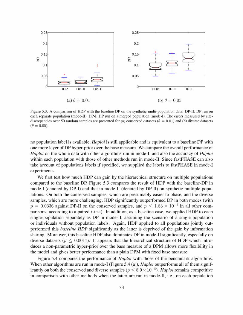
HDP DP−II DP−I0

0.05

0.1

0.15

0.2

0.25

err

HDP DP−II DP−I0

0.05

0.1

0.15

0.2

0.25

err

(a) θ = 0.01 (b) θ = 0.05

Figure 5.3: A comparison of HDP with the baseline DP on the synthetic multi-population data. DP-II: DP run oneach separate population (mode-II). DP-I: DP run on a merged population (mode-I). The errors measured by site-discrepancies over 50 random samples are presented for (a) conserved datasets (θ = 0.01) and (b) diverse datasets(θ = 0.05).

no population label is available, Haploi is still applicable and is equivalent to a baseline DP withone more layer of DP hyper-prior over the base measure. We compare the overall performance ofHaploi on the whole data with other algorithms run in mode-I; and also the accuracy of Haploiwithin each population with those of other methods run in mode-II. Since fastPHASE can alsotake account of populations labels if specified, we supplied the labels to fastPHASE in mode-Iexperiments.

We first test how much HDP can gain by the hierarchical structure on multiple populationscompared to the baseline DP. Figure 5.3 compares the result of HDP with the baseline-DP inmode-I (denoted by DP-I) and that in mode-II (denoted by DP-II) on synthetic multiple popu-lations. On both the conserved samples, which are presumably easier to phase, and the diversesamples, which are more challenging, HDP significantly outperformed DP in both modes (withp = 0.0336 against DP-II on the conserved samples, and p ≤ 1.83 × 10−6 in all other com-parisons, according to a paired t-test). In addition, as a baseline case, we applied HDP to eachsingle-population separately as DP in mode-II, assuming the scenario of a single populationor individuals without population labels. Again, HDP applied to all populations jointly out-performed this baseline HDP significantly as the latter is deprived of the gain by informationsharing. Moreover, this baseline HDP also dominates DP in mode-II significantly, especially ondiverse datasets (p ≤ 0.0017). It appears that the hierarchical structure of HDP which intro-duces a non-parametric hyper-prior over the base measure of a DPM allows more flexibility inthe model and gives better performance than a plain DPM with fixed base measure.

Figure 5.4 compares the performance of Haploi with those of the benchmark algorithms.When other algorithms are run in mode-I (Figure 5.4 (a)), Haploi outperforms all of them signif-icantly on both the conserved and diverse samples (p ≤ 8.9×10−5). Haploi remains competitivein comparison with other methods when the latter are run in mode-II, i.e., on each population

33

fPh Ph Ma Be fPh Ph Ma Be−0.05

0

0.05

0.1er

r −

err

(HD

P)

θ=0.01 θ=0.05fPh Ph Ma Be fPh Ph Ma Be

−0.05

0

0.05

0.1

err

− e

rr(H

DP

)

θ=0.01 θ=0.05

(a) Mode-I (b) Mode-II

Figure 5.4: A comparison of HDP with other algorithms (fPh:fastPHASE, Ph:Phase, Ma:Mach, Be:Beagle) runningin (a) mode-I, and (b) mode-II, on synthetic multi-population data.

separately (Figure 5.4 (b)). On the conserved data, PHASE shows the best result, but the differ-ences between algorithms are not significant (p ≤ 0.11). Whereas on the diverse data, Haploioutperforms other algorithms significantly (p ≤ 0.0043).

5.4.3 Parameter estimation and sensitivity analysisTypically, with random initialization, the Gibbs sampler for Haploi converges within 1000 it-eration on the synthetic data. This contrasts sampling algorithms used in some of the otherhaplotype models, which typically need tens of thousands of iterations to reach convergence.The fast convergence is possibly due to Haploi’s ability to quickly infer the correct number offounding haplotypes underlying the genotypes samples, which leads to a model significantlymore compact (i.e., parsimonious) than that derived from other methods.

Estimating K and θ

We compared the estimated K— the number of recovered ancestors via both HDP and DP mix-tures. Recall that we expect K to be 17. Overall, the estimated K under both the DP and HDPmodels turns out to be very close to this number on the conserved datasets. From the diversedatasets, HDP can still offer a good estimate of the number of ancestors, whereas DP recov-ered more ancestors (around 25 on average) than the true number. This is not surprising since ahaplotype which appears in more than one population can have different frequencies in differentpopulations, the baseline DP cannot capture such sub-population structure, and the higher diver-gence due to both mutation and population diversification can make it generate more ancestorsto describe the given dataset.

Our Gibbs sampler also provides reasonable estimates of the mutation rates of each haplotypefounder. We observe that for the conserved data sets, HDP yields highly consistent and low

34

Table 5.1: A sensitivity analysis to the hyper-parameters of HDP on conserved dataset. Result with different hyper-parameters ι and κ for inverse Gamma prior is shown. The number of founders for each population (Ki) and thetotal number of ancestors across all the populations are shown in columns 4–9. The estimated mutation rate θ andthe haplotyping errors (errs) are also shown through columns 10 – 11. The sensitivity of θ estimate to the hyperprior is examined over a wide range of both different magnitudes (0.1 to 1000) and ratios (0.0001 to 10000) of ι andκ.

κ ι κ/ι K1 K2 K3 K4 K5 total K (17) θ (0.005) errs0.1 0.1 1 5.0 5.0 5.0 5.0 5.0 17.8 0.005 0.0058

0.5 0.2 5.0 5.0 5.0 5.0 5.0 17.5 0.004 0.01161 0.1 5.0 5.0 5.0 5.0 5.0 18.0 0.004 0.0000

10 0.01 5.0 5.0 5.0 5.0 5.0 18.0 0.004 0.0087100 0.001 5.0 4.0 5.0 5.0 4.0 16.0 0.007 0.0029

1000 0.0001 5.0 5.0 5.0 5.0 4.0 17.0 0.004 0.00290.5 0.1 5 5.0 5.1 5.0 5.0 5.0 18.1 0.004 0.0087

0.5 1 5.0 4.1 5.0 5.0 5.0 17.1 0.007 0.00291 0.5 5.0 5.0 5.0 5.0 5.0 18.0 0.004 0.0029

10 0.05 5.0 5.0 5.0 5.0 5.0 18.0 0.004 0.0145100 0.005 5.0 5.0 5.0 5.0 4.0 17.0 0.004 0.0029

1000 0.0005 5.0 5.0 5.0 5.0 4.0 17.0 0.005 0.00871 0.1 10 5.0 5.0 5.0 6.0 5.0 18.0 0.006 0.0116

0.5 2 5.0 5.0 5.0 5.0 5.0 18.0 0.004 0.00581 1 5.0 5.0 5.0 5.0 5.0 18.0 0.004 0.0087

10 0.1 5.0 5.0 5.0 5.0 5.0 18.0 0.004 0.0029100 0.01 5.0 4.0 5.0 5.0 4.0 16.0 0.007 0.0087

1000 0.001 5.0 4.9 5.0 5.0 4.0 16.9 0.005 0.008710 0.1 100 5.0 5.0 5.0 5.3 5.0 17.1 0.004 0.0000

0.5 20 5.0 5.0 5.0 5.0 5.0 18.0 0.004 0.00871 10 5.0 5.0 5.0 5.0 5.0 18.1 0.004 0.0029

10 1 5.0 5.0 5.0 5.0 5.0 18.0 0.004 0.0000100 0.1 5.0 4.0 5.0 5.0 5.0 17.0 0.007 0.0058

1000 0.01 5.0 5.0 5.0 5.0 4.0 17.0 0.004 0.0087100 0.1 1000 5.8 5.5 5.6 6.1 6.0 18.2 0.010 0.0116

0.5 200 5.2 5.2 5.2 5.8 5.5 18.4 0.008 0.01161 100 5.1 6.2 5.4 5.5 5.2 17.3 0.006 0.0087

10 10 5.0 5.0 5.1 5.0 5.1 18.1 0.005 0.0029100 1 5.0 5.0 5.0 5.0 5.0 18.0 0.004 0.0000

1000 0.1 5.0 5.0 5.0 5.0 4.0 17.0 0.004 0.00001000 0.1 10000 6.8 6.3 8.5 6.0 10.3 25.6 0.003 0.0087

0.5 2000 7.1 7.0 7.4 6.6 8.5 24.5 0.006 0.01161 1000 6.4 6.5 7.7 6.4 8.4 22.8 0.005 0.0145

10 100 5.3 6.5 6.3 5.8 7.0 17.8 0.010 0.0260100 10 5.1 5.1 5.0 5.0 5.1 18.1 0.005 0.0087

1000 1 5.0 5.0 5.0 5.0 5.0 18.0 0.004 0.0029

35

variance estimations of θ, and the quality of the estimates due to DP is slightly worse. For thediverse data both algorithms tend to slightly underestimate the mutation rates, and the varianceis also higher. It is noteworthy that in principal, high haplotype diversity of a population canbe explained by two competing sources: high mutation rate from ancestors to descendants, andlarge number of ancestors. Indeed K and θ cannot be independently determined, following asimilar argument of the un-identifiability of the evolution time and population size under IAMmodel. But empirically, HDP appears to strike a reasonable balance between K and θ, and offersplausible estimates of both.

A more thorough sensitivity analysis with respect to the hyper-parameters in our model isdetailed in Table 5.1. The proposed HDP model has two scale parameters, γ and τ , for the upperand lower level DP, which are under inverse Gamma priors as discussed in Section 5.2.2. Tosee the sensitivity of the K and θ estimations under different priors, we applied various valuesof hyper parameters ι and κ (the same for both γ and τ ) on one of the 50 random conserveddatasets. Columns 4 – 9 in Table 5.1 show the number of recovered founders within each sub-population (the correct number is 5 for each), and the total number of distinct founders over allthe populations. Overall, over a wide range of values for the hyper-parameters, Haploi giveslow-bias and low-variance estimation of the number of founders of each sub-population as wellas the total number of distinct founders. In columns 10-11, we show the inferred mutation rateand the haplotyping error. Even when incorrect numbers of founders are recovered, the actualhaplotyping errors are not significantly affected, which shows the robustness of the proposedapproach for haplotype recovering application. The test on the diverse dataset shows similartendency while the result is slightly less stable (see Table A.1 in Appendix for more details).

Estimating haplotype frequencies

Figure 5.5 summarizes the accuracy of population haplotype frequencies estimated by each al-gorithm. The discrepancy between the true frequencies and estimated ones is measured by theKL-Divergence DKL(p||q) =

∑x p(x) log p(x)

q(x). The top row shows the accuracy of HDP along

with those of DP in mode-II and in mode-I, and the bottom row shows the comparison of HDPwith other benchmark algorithms. The left column of Figure 5.5 (a) reports DKL computed onALL haplotypes frequencies estimated by different algorithms from the conserved data sets andthe right column of Figure 5.5 (a) shows the result when measured only on the frequent haplo-types (i.e., with frequencies ≥ 0.05). Comparing to the baseline-DP, HDP is as accurate whenonly frequent haplotypes are considered. When all the frequencies are considered, however,the margin of HDP over DP becomes significant, especially on the diverse dataset (p=0.0009).Overall,Haploi, PHASE, and MACH work equally well without significant difference in perfor-mance on conserved datasets. For more difficult diverse data sets (Figure 5.5 (b)), HDP achievesthe lowest discrepancy by a significant margin over all the other algorithms. The runner-up,PHASE beats fastPHASE and MACH with a small margin. When measured only on the frequenthaplotypes (i.e., the right column of Figure 5.5 (b)), the discrepancies decrease significantly, butthe relative ordering of all the compared algorithms remains similar, except that now fastPHASEoutperforms PHASE (p = 0.0036).

36

HDP DP−II DP−I0

0.5

1

1.5

2

err

Haplotype frequency error (DKL

)

(with all frequencies )

HDP DP−II DP−I0

0.5

1

1.5

2


)

(with frequencies >= 0.05)

fPh Ph Ma Be

−0.5

0

0.5

1

err

− e

rr(H

DP

)

fPh Ph Ma Be−0.1

0

0.1

0.2

(a)

HDP DP−II DP−I0

0.5

1

1.5

2


)

(with all frequencies)

HDP DP−II DP−I0

0.5

1

1.5

2


)

(with frequencies >= 0.05)

fPh Ph Ma Be

−0.5

0

0.5

1

fPh Ph Ma Be−0.1

0

0.1

0.2

(b)

Figure 5.5: A comparison of the accuracies of haplotype frequencies. Top: the result from HDP, DP in mode-II(DP-II), and DP in mode-I (DP-I). Bottom: the result from HDP and three benchmark algorithms. (a) Box-plots ofDKL’s estimated from the conserved data sets. Left column shows measurements on all haplotypes, right columnshows measurements on only the frequent haplotypes. (b) Same measurements on the diverse datasets.

37

5.4.4 Result on HapMap Data

We also test Haploi on both short SNP segments (i.e., ∼ 6 SNPs), and long SNP sequences(i.e., ∼ 102 − 103 SNPs) available from the International HapMap Project. This data containsSNP genotypes from four populations: Utah residents with ancestry from northern and westernEurope (CEU); Yoruba in Ibadan, Nigeria (YRI); Han Chinese in Beijing (CHB); and Japanesein Tokyo (JPT), with 60, 60, 45, and 44 unrelated individuals, respectively. Although haplotypeinference can be, and in some test scenarios, was performed on all populations, evaluation ofthe outcome is on only the CEPHs and Yorubas since the true haplotypes can be almost un-ambiguously deduced from trios only in these two populations. The individual genotypes thatcannot be unambiguously phased from the trios were ignored in the scoring. We consider threedifferent population-composition scenarios in our experiments below: 1) using all the four popu-lations together for haplotype inference (FourPop); 2) using only CEPH and Yoruba populationsfor inference (TwoPop); and 3) phasing CEPH and Yoruba separately (OnePop). Essentially, inthe FourPop and TwoPop scenarios we solve a bigger haplotype inference problem on data thatcontain richer population information.

Short SNP sequences

Phasing short SNPs is the basic operation of large-scale haplotype inference problems that relyeither on a partition-ligation heuristic, or on a model-based methods, such as recombination pro-cesses, to integrate short phased haplotype segments into long haplotypes. Figure 5.6 shows acomparison of the phasing accuracy on 6-SNP segments (following a recommendation in Niuet al. (2002) on the optimal size-range of basic units for subsequent ligation) by four algorithms.The test was done on randomly selected 100 sets of 6-SNPs segment from chromosome 21. Foreach of the three population-composition scenarios, we applied all methods to different popula-tion sizes, i.e., 60, 30, 20, and 10 individuals per population, to examine the effect of populationsize on phasing accuracy.

Several aspects of Haploi’s performance on real data are revealed by Figure 5.6. First, com-paring the performances of Haploi under the three different population-composition scenarios,we observe that Haploi improves steadily as more populations are included in haplotype infer-ence, and the improvements are statistically significant. The p-values of the differences betweenFourPop and OnePop scenarios are 0.00024, 0.000038, 0.0016, and 0.000022 for data with 60,30, 20, 10 individuals per population, respectively; and the p-values of the margins of TwoPopover OnePop are 0.0014, 0.0002, 0.0053, and 0.00047, respectively, in the same order. Theimprovement in FourPop over TwoPop is less significant, with p-values 0.35, 0.11, 0.16, and0.023, respectively, suggesting that the possible gain in haplotype accuracy enabled by the HDPmodel via exploring shared information among populations can be capitalized the most when wechange from single-population inference to joint-inference in multiple population; whereas theeffect of having more populations in the multi-population scenario appears to be less obvious inthis dataset.

Second, comparing the performances of Haploi under different population sizes, we observethat the performance-gain through information sharing among populations tends to be greaterwhen the population sizes decrease. For example, the performance differences of Haploi in

38

multi-population over single-population become most significant when the number of individualsper population is the smallest (#Individual per pop=10). This observation suggests that HDP isespecially advantageous under data scarcity situation where information from each populationbecomes insufficient to warrant reliable inference within the population.

Third, other methods such as PHASE, MACH, and Beagle, appear not able to benefit fromincreased population diversity as indicated by the significant drop of their accuracies when morepopulations are involved. The performance of fastPHASE (with known population labels) im-proves substantially when two populations are used together, while the performance becomesslightly worse in the case of four populations. Comparing the results from the most preferredscenario of each algorithm, that is, Haploi under FourPop, fastPHASE under TwoPop, and allthe others under OnePop, Haploi and PHASE worked similarly well when all the available datawere used (i.e. #Individual per pop=60), with mean error rate of each algorithm at 0.0174,0.0198, 0.0173, 0.0229, and 0.0222, respectively (with p =0.05,0.89,0.10,0.01 over differencesof Haploi with other algorithms). When the population sizes decrease, Haploi starts to surpassothers more substantially, and works more reliably than others. For example, on 10 individualsper population, the mean error rates of the five algorithms were 0.0424, 0.0460, 0.0512, 0.0777,and 0.0945, and the p-values of the margin of Haploi over others are 0.17, 0.02, 1.2 × 105,6.7× 106, respectively.

Long SNP sequences

Finally we test Haploi on very long genotype sequences with 102 ∼ 103 SNPs. We selected 10ENCODE regions from the HapMap DB, each spanning roughly 500 Kb and containing from 254to 972 common SNPs across all four populations (see Table A.2 in Appendix for more details).We performed haplotype inference under three different population-composition scenarios asbefore, but due to the extremely high cost in computational time in these experiments, we onlyworked on the full-size data sets. Figure 5.7 shows a comparison of haplotype reconstructionquality, using PHASE, fastPHASE, MACH, Beagle and Haploi equipped with the PL heuristic 1.Out of the 30 experiments we performed (10 regions and three scenarios), the PHASE programfailed to yield results in 5 experiments after a 31-day runtime, so we omit the correspondingresults in our summary figure.

The conclusion from Figure 5.7 is less clear than the ones from previous sections from ex-periments on short SNP sequences and on simulation data. Overall, Beagle dominates all thealgorithms with a small margin, PHASE also shows comparable result to Beagle when con-verged, but all the other algorithms work comparably in most cases across different datasets anddifferent scenarios. In terms of computational cost, Beagle was the fastest, it took less than aminute for each task; fastPHASE and MACH mostly took less than 1 hour for each task, Haploitook from 1-10 hours, depending on the length of the sequence; whereas PHASE took one to twoorders of magnitude longer, and was indeed impractical for phasing very long sequence.

In summary, our result shows that Haploi is competent and robust for phasing long SNP se-quences from diverse genetic origins at reasonable time cost, even though it has not yet employed

1We could not get output of PHASE for these long sequences within acceptable running time (> 800hours).Instead we included fastPhase result, which is said to be much faster than PHASE with a slight performance degra-dation (Scheet and Stephens, 2006).

39

any sophisticated way for processing long sequences, such as the recombination process. SinceHaploi appeared to outperform other methods over short SNPs, we believe that the competenceof Haploi on long SNPs is due to a better inference power endowed by the HDP model for multi-population haplotypes; and we expect that an upgrade that incorporates explicit recombinationmodels in conjunction with HDP for long SNPs are likely to lead to more accurate haplotypereconstructions.

5.5 DiscussionWe have proposed a new Bayesian approach to haplotype inference for multiple populationsusing a hierarchical Dirichlet process mixture. By incorporating an HDP prior which couplesmultiple heterogeneous populations and facilitates sharing of mixture components (i.e., founderhaplotypes) across multiple Dirichlet process mixtures, the proposed method can infer the truehaplotypes in a multi-ethnic group with an accuracy superior to the state-of-the-art haplotypeinference algorithms.

There emerged new models related to our HDP model, the closest being the nested Dirichletprocess (NDP) by Rodriguez et al. (2006). In an NDP, instead of using a hyper-DP as a commonbase measure as in HDP to allow sharing of founders across populations, the population-specificDPs are directly drawn from a prior DP, so that not only the founders, but also their frequenciescan be shared across populations. Although this model can be more expressive in many appli-cations, it may be less appropriate than HDP for multi-population haplotype problems whereexcessive structural sharing across populations is not warranted, especially when different pop-ulations bear very distinct demography and genetic prototypes. Another strategy proposed byMuller et al. (2004) employs an explicit stochastic convex combination of a population-specificprior and a universal prior for each founder. Under such a model, once a founder is destined to beshared across populations, it will appear with equal frequency in all populations. HDP subsumesthis scenario, but also allows more flexible sharing of the founders.

The proposed model achieves the desirable properties of PAC regarding mutation dynamics(Li, 2003), including the parental-dependent-mutation effect, albeit in a very different way. Forexample, to see the PDM property, note that when a next haplotype is to be sampled accord-ing to Equation (3.4), we pick an ancestor of some previously drawn haplotypes, and apply amutation process to the ancestor, rather than to one of the previously drawn haplotypes as inPAC. This operation implicitly results in a PDM effect among haplotypes by relating them totheir corresponding founder via a tractable star genealogy equipt with a common mutation pro-cess Ph(|founder). A new haplotype generated from this process will bear mutations over itscorresponding founders rather than been completely random. Above these founders, we modeltheir genealogy and type history by a coalescent-with-IMA model, whose resulting marginal isequivalent to that of the Dirichlet process. Here a new founder can be sampled independentof the type-history in the coalescent from the base measure, rather than according to a PDM,with probability proportional to the IMA mutation rate. Putting everything together, the DPmixture model essentially implements a combination of IMA and PDM: it models the geneal-ogy and type history of hypothetical ancestors presumably corresponding to a bottleneck with acoalescent-with-IMA model; below the bottleneck, it uses multiple (indeed, can be countably in-

40

finite many) star genealogies rooted at the ancestors present in the bottleneck and equipt with anancestor-dependent Poisson mutation process, to approximate the coalescent-with-PDM model.The time of the bottleneck depends on the value of the scaling parameter α of the DP. One canintroduce a prior to this parameter so that it can be estimated a posteriori from data.

It is well-known that under Kingman’s n-coalescent, a dominant portion of the depth of thecoalescent tree is spent waiting for the earliest few lineages to coalesce to the MRCA and themajority of lineages of even a very large population can actually coalesce very rapidly into afew ancestors, which means that the net mutation rates from each of these ancestors to theirdescendants in a modern haplotype sample do not vary dramatically among the descendants.Thus qualitatively a star genealogy provides a reasonable approximation to the actual (heavilytime-compressed) genealogy of a modern haplotype sample up to these ancestors. As a rewardof such approximation, a well-known property of DP mixture is that it defines an exchangeabledistribution of the samples. Furthermore, the Polya urn construction of DP enables simple andefficient Monte Carlo for posterior inference of haplotypes and other parameters of interest, andthe DPM formalism offers a convenient path for extensions that capture more complex demo-graphic and genetic scenarios of the sample, such as the multi-population haplotype distributionas we explored.

Unlike the models underlying PHASE and fastPhase, the PL heuristic used in the Haploiprogram does not explicitly model the recombination process that shapes the LD patterns of longSNP sequences. Since an HDP model without the aid of the PL-scheme dominates PHASE andfastPhase over short SNPs, we believe that an upgrade that incorporates an explicit recombina-tion model in conjunction with HDP is likely to lead to more accurate reconstruction of longhaplotypes. The hidden Markov Dirichlet process recently developed by us to model recombina-tion in open ancestral space offers a promising path for such an upgrade (Xing and Sohn, 2007).Under the proposed statistical framework for modeling haplotype and genotype distribution, itis also straightforward to handle various missing value problems in a principled way. In anotherpossible extension, although in the present study we have assumed that the population labels ofindividuals are known, it is straightforward to generalize our method to situations in which theethnic group labels are unknown and to be inferred. This opens the door to applications of ourmethod to large-scale genetic studies involving joint inference over markers and demography.The HDP model is also a natural formalism for applications outside of population genetics, suchas in text modeling, where one can use an HDPM to model co-clustering of documents fromdifferent journals (analogous to different populations here) according to both shared and uniquetopics defined by, e.g, a latent Dirichlet allocation model (Blei et al., 2003); and also in networkmodeling, where the neighbor profiles of every node can be modeled by a low-level DPM whoselikelihood function is defined by, e.g., a mixed membership stochastic block model (Airoldi et al.,2006), and the entire network corresponds to an HDP over all nodes.

41

Four pops Two pops One pop

HDP fPh Ph Ma Be0

0.2

0.4

0.6

0.8

#Individual per pop=60

HDP fPh Ph Ma Be0

0.2

0.4

0.6

0.8


HDP fPh Ph Ma Be0

0.2

0.4

0.6

0.8


HDP fPh Ph Ma Be0

0.2

0.4

0.6

0.8


Figure 5.6: A comparison of haplotyping error on CEPH+Yoruba population over randomly chosen 100 sets of6-SNP segments from Chromosome 21. The results were obtained under three population-composition scenarios:(i) FourPops: when data from all the four populations were used (blue) for inference; (ii) TwoPops: when data fromCEPH and Yoruba populations were used together (green); (iii) OnePop: when each of CEPH and Yoruba populationwas used separately (gray). Different sample sizes, with 60, 30, 20, and 10 individuals per each population, wereused.

42

HDP fPh Ph Ma Be0

0.05

0.1

0.15

0.2~~

NA

HDP fPh Ph Ma Be0

0.05

0.1

0.15

0.2~~

NA~~

NA

HDP fPh Ph Ma Be0

0.05

0.1

0.15

0.2~~

NA~~

NA

(a) (b) (c)

Figure 5.7: Performance on the full sequences of the selected ten ENCODE regions. (a) Error rates under fourpopulation scenario (b) Under the two-population scenario. (c) Under the one population scenario. For cases ofwhich the program does not converge (NC) within a tolerable duration (i.e., 800 hours), we cap the bar with a “≈”to indicate that the results are not available (NA).

43

Chapter 6

Joint inference of population structure andrecombination events

6.1 Introduction

SNPs are remnants of ancient DNA alterations dated back to a time measured at a genealogi-cal scale. They contain finer-grained information on molecular evolution than that revealed byorthologous genomic sequences from multiple species. In general, the higher the frequency ofa SNP allele, the older the mutation that produced it, so high-frequency SNPs largely predatehuman population diversification whereas low-frequency ones appeared afterwords. Therefore,population-specific alleles may bear important information about human evolution such as spe-cific migrations and genetic diversifications (Stoneking, 2001).

A number of variants of statistical admixture models for genetic polymorphisms have beenproposed for the analysis of current population structure (Falush et al., 2003; Pritchard et al.,2000; Rosenberg et al., 2002). These models are instances of a more general class of hierarchicalBayesian models known as mixed membership models (Erosheva et al., 2004), which postulatethat genetic markers of each individual are iid (Pritchard et al., 2000) or spatially coupled (Falushet al., 2003) samples from multiple population-specific fixed-dimensional multinomial distribu-tions (known as ancestry proportions (Falush et al., 2003), or AP) of marker alleles. Under thisassumption, the admixture model identifies each ancestral population by a specific AP (that de-fines a unique allele frequency profile for each ancestral population for each marker) and displaysthe fraction of contributions from each AP in a modern individual chromosome as a structuralmap. Fig. 6.1 shows an example of structural maps of four modern populations inferred from aportion of the HapMap multi-population dataset by Structure 2.1 (Falush et al., 2003; Pritchardet al., 2000). In this population structural map, each individual is represented as a thin verti-cal line which shows the fraction of the individual’s chromosome which originated from eachancestral population, as given by a unique AP.

However, since an AP merely represents the frequency of alleles in an ancestral population,rather than the actual allelic content or haplotypes of the alleles themselves, the admixture modeldoes not model genetic drift due to mutations from the ancestral alleles. Moreover, in the extantadmixture models, the correlations between loci along the chromosome are only captured by the

45

Figure 6.1: Population structural map inferred by Structure 2.1 on HapMap multi-population data consisting ofCEU, YRI, HCB and JPT populations.

linkage disequilibrium due to variation in the AP fractions over all markers among individuals,or due to a “recombination” process between APs , rather than ancestral chromosomes, for sam-pling markers along a modern chromosome. These two scenarios are known as “mixture LD”and “admixture LD” respectively (Falush et al., 2003). Neither one captures the actual recombi-nation events at the ancestral chromosome level, so they do not enable inference of the foundinggenetic patterns, the recombination events, the age of the founding alleles, or the composition ofindividual chromosomes at founding chromosome level (Excoffier and Hamilton, 2003). Actu-ally, while this model aims to provide ancestry information for each individual and each locus,there is no explicit representation of “ancestors” as a real chromosome haplotype. Therefore, theinferred population structural map emphasizes revealing the contributions of abstract population-specific ancestral proportion profiles, which does not directly reflect individual diversity. Thisrepresentation may not be optimal, as seen in Figure 6.1: each modern population is representedby a very homogenous, but distinct population structural sub-map, which reflects little about theactual genetic diversity of each population and individual and little about the relative similaritybetween populations. For example, the YRI population from Africa is known to be geneticallydiverse, but in Figure 6.1 it appears to be the most homogeneous.

We have presented a new method, Spectrum, for inferring and representing population struc-tures, using a unified statistical framework for modeling the genetic inheritance process thatallows both recombination among an unspecified number of founding haplotypes and mutationsfrom these founders. Based on this model, which represents a well-defined generative model forthe observed chromosomes, we represent the population structure in terms of an ancestral spec-trum which shows the ancestral composition of each modern individual chromosome in termsof its origin among the chromosomal ancestors. By considering the different ancestral associa-tion patterns among populations, this spectrum helps to separate the sub-populations, as well asreveal the diversity among individuals and populations. Moreover, our model allows us to re-cover the recombination events in each individual chromosome. In fact, the population structurecan play an important role for the LD analysis. Figure 6.2 shows the LD measurements for allpairwise loci on the ENm010 region from HapMap DB. When we compute LD in three popula-tions of CEU (European ancestry), HCB and JPT (Asian ancestry) together (Figure 6.2(a)), somedegree of block-like patterns are visible, but when CEU (European ancestry) and YRI (Africanancestry) populations are mixed (Figure 6.2(b)), the block structure is less obvious. This re-sult implies the existence of different genetic processes in the evolutionary history of the twopopulations. Hence, if we perform LD or recombination analysis on a population which may

46

(a) CEU + HCB + JPT (b) CEU + YRI

Figure 6.2: The LD measurements, |D′| (upper right), and the p-values for Fisher’s exact test (lower left), of HapMapDB (Thorisson et al., 2005). In each of the LD maps, starting from the upper-left corner, all the markers are listed intop-down and left-right directions, and each marker is at a spatial position corresponding to its actual genetic distancewith respect to the first marker at the upper-left corner. Note the LD-block structures on the mixed populations ofCEU and YRI in shown (b) are rather opaque compared to the LD patterns of CEU+HCB+JPT populations in (a).

have a concealed sub-population structure, it would be more informative to perform LD analy-sis on each sub-population separately, and our ancestral spectrum offers a way to classify suchsub-populations on genetic basis. While the statistical methodologies developed so far mostlydeal with ancestral inference and LD analysis separately using specialized models that do notcapture the close statistical and genetic relationships of these two problems, we propose a uni-fied framework which allows joint inference of the population structure and the recombinationpatterns.

We assume that individual chromosomes in a modern population originated from a numberof ancestral chromosomes via biased random recombination and mutation. By associating eachancestor with a hidden state, the recombination between the ancestors can follow a state transitionprocess, and the mutation can follow an emission process in the hidden Markov model. Henceeach individual chromosome can be thought of as a “mosaic” of ancestral chromosomes underthis model.

Several existing methods have employed similar ideas. For example, Daly et al. (2001) andGreenspan and Geiger (2004) have developed hidden Markov models for locating recombina-tion hotspots in haplotypes; Anderson and Novembre (2003) proposed a minimum descriptionlength (MDL) method for optimal haplotype block finding. While these models are based on asimilar assumption that each observed haplotype is a “mosaic” of ancestral haplotypes and theformation of the mosaic is governed by a hidden Markov process over the ancestor space, theseHMMs cannot be used easily to infer individual recombination events because the block bound-aries which conceptually correspond to the recombination sites of all individual chromosomesare decided outside the model via model selection, and the only intrinsic stochasticity lies inthe choice of the “ancestors” at each block for each chromosome rather than the genomic loca-

47

tions of recombination events in each chromosome. It is also unclear to what extent this classof approaches might be helpful for applications involving explicit ancestral map inference asin Rosenberg et al. (2002) and for interpreting LD patterns that do not have sharp block bound-aries as in Figure 6.2(b).

While most of the previous approaches ignore the inherent uncertainty in the genetic com-plexity (e,g., the number of genetic founders of a population) of the data, our new approachemploys a non-parametric Bayesian model of infinite hidden Markov model which we call Hid-den Markov Dirichlet Process to extend a closed genetic inheritance model based on a fixednumber of founders to an open ancestral space, which allows more flexible control over the num-ber of genetic founders than has been provided by the statistical methods proposed thus far. Wereport validation of Spectrum on both simulated data and on two real datasets of HapMap andDaly data, and compare with a number of established methods.

6.2 The statistical modelWe describe a statistical model for generating individual haplotypes in a modern populationfrom a hypothetical pool of ancestral haplotypes via recombination and mutations. We beginour exposition with a parametric Bayesian model of genetic inheritance involving recombinationand mutation over a fixed number of ancestors; then we extend the model to open ancestral spacewhich requires no ad hoc specification of the number of ancestors, via a nonparametric Bayesianapproach.

6.2.1 Hidden Markov model for recombination and mutation in closed an-cestral space

We begin with the assumption that modern chromosomes are derived from ancestral chromo-somes via biased random recombination and mutation. This assumption corresponds to an ideal-ized noninterference model for chromosomal crossover and a star genealogy over every inheritedsite. If the number of ancestors is known to be K, sequential selection of recombination targetsfrom a set of ancestral chromosomes can be modeled as a hidden Markov process, where thehidden states correspond to the founders, the transition probabilities correspond to the recombi-nation rates between the recombining chromosome pairs, and the emission model corresponds toa mutation process that passes the chosen chromosome in the founders to the descendants.

Assuming that individual haplotypes over T SNPs Hie = [Hie,1, . . . , Hie,T ] for e = 1, 2 aregiven unambiguously for the study population, as is the case in many LD and haplotype-blockanalyses (Anderson and Novembre, 2003; Daly et al., 2001), we can now treat the paternal andmaternal haplotypes of N individual as 2N iid samples and omit the parental index e. Althoughthis assumption may seem stringent, our model can easily generalize to unphased genotype databy incorporating a simple genotype model, as will be explained later in this section.

Now, let Ak = [Ak,1, . . . , Ak,T ] for k = 1, . . . , K be the K ancestral haplotypes, and letCi = [Ci,1, . . . , Ci,T ] denote the sequence of inheritance variables that specify the index of theancestral chromosome at each SNP locus for each chromosome i. Also suppose that the transi-tion probabilities of the HMM are given as a K × K matrix π. When no recombination takes

48

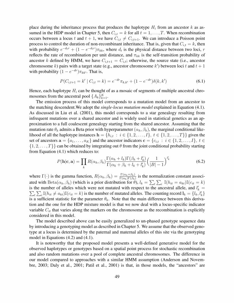
place during the inheritance process that produces the haplotype Hi from an ancestor k as as-sumed in the HDP model in Chapter 5, then Ci,t = k for all t = 1, . . . , T . When recombinationoccurs between a locus t and t + 1, we have Ci,t 6= Ci,t+1. We can introduce a Poisson pointprocess to control the duration of non-recombinant inheritance. That is, given that Ci,t = k, thenwith probability e−dtr + (1 − e−dtr)πkk, where dt is the physical distance between two loci, rreflects the rate of recombination per unit distance, and πkk is the self-transition probability ofancestor k defined by HMM, we have Ci,t+1 = Ci,t; otherwise, the source state (i.e., ancestorchromosome k) pairs with a target state (e.g., ancestor chromosome k′) between loci t and t+ 1with probability (1− e−dr)πkk′ . That is,

P (Ci,t+1 = k′ | Ci,t = k) = e−drπk,k′ + (1− e−dr)δ(k, k′) (6.1)

Hence, each haplotype Hi can be thought of as a mosaic of segments of multiple ancestral chro-mosomes from the ancestral pool {Ak}Kk=1.

The emission process of this model corresponds to a mutation model from an ancestor tothe matching descendent.We adopt the single-locus mutation model explained in Equation (4.1).As discussed in Liu et al. (2001), this model corresponds to a star genealogy resulting frominfrequent mutations over a shared ancestor and is widely used in statistical genetics as an ap-proximation to a full coalescent genealogy starting from the shared ancestor. Assuming that themutation rate θk admits a Beta prior with hyperparameter (αh, βh), the marginal conditional like-lihood of all the haplotype instances h = {hi,t : i ∈ {1, 2, . . . , I}, t ∈ {1, 2, . . . , T}} given theset of ancestors a = {a1, . . . , aK} and the ancestor indicators c = {ci,t : i ∈ {1, 2, . . . , I}, t ∈{1, 2, . . . , T}} can be obtained by integrating out θ from the joint conditional probability startingfrom Equation (4.1) which reduces to:

P (h|c, a) =∏k

R(αh, βh)Γ(αh + lk)Γ(βh + l′k)

Γ(αh + βh + lk + l′k)

( 1

|B| − 1

)l′k(6.2)

where Γ(·) is the gamma function, R(αh, βh) = Γ(αh+βh)Γ(αh)Γ(βh)

is the normalization constant associ-ated with Beta(αh, βh) (which is a prior distribution for θ), lk =

∑t

∑i I(hit = akt)I(cit = k)

is the number of alleles which were not mutated with respect to the ancestral allele, and l′k =∑t

∑i I(hit 6= akt)I(cit = k) is the number of mutated alleles. The counting record lk = {lk, l′k}

is a sufficient statistic for the parameter θk. Note that the main difference between this deriva-tion and the one for the HDP mixture model is that we now deal with a locus-specific indicatorvariable Cit that varies along the markers on the chromosome as the recombination is explicitlyconsidered in this model.

The model described above can be easily generalized to un-phased genotype sequence databy introducing a genotyping model as described in Chapter 5. We assume that the observed geno-type at a locus is determined by the paternal and maternal alleles of this site via the genotypingmodel in Equations (4.2) and (4.1).

It is noteworthy that the proposed model presents a well-defined generative model for theobserved haplotypes or genotypes based on a spatial point process for stochastic recombinationand also random mutations over a pool of complete ancestral chromosomes. The difference inour model compared to approaches with a similar HMM assumption (Anderson and Novem-bre, 2003; Daly et al., 2001; Patil et al., 2001) is that, in those models, the “ancestors” are

49

defined independently for each block rather than as whole chromosomes, which is biologicallyless meaningful. Although such a generative process is still a simplification of the real biolog-ical mechanism, it enables the joint statistical characterization of a number of genetic variablesof interest, via posterior inference based on well-founded statistical principles, and it strikes areasonable tradeoff between being biologically meaningful and computationally manageable.

6.2.2 Hidden Markov Dirichlet Process for Inheritance in open ancestralspace

So far, we have been assuming that recombination and mutation take place in a closed ancestralspace; that is, the number of ancestral chromosomes is known a priori. But this assumption,which is also widely adopted in other existing approaches for LD analysis and ancestral infer-ence, ignores the inherent uncertainty in the genetic complexity of populations. Model selectionaccording to information theoretic score or Bayes factors is a typical solution to problems of thisnature, but it can be inflexible when the hypothesis space is large. We have developed a nonpara-metric Bayesian framework for modeling genetic polymorphism based on the Dirichlet process(DP) mixtures and extension (Sohn and Xing, 2007a,b; Xing et al., 2004; Xing and Sohn, 2007),which allows more flexible control over the number of genetic founders.

Using an infinite Hidden Markov model which we also call the Hidden Markov DirichletProcess (HMDP) (Sohn and Xing, 2007a,b; Xing and Sohn, 2007), we extend the HMM modelproposed in Section 6.2.1 to work in an infinite ancestral space. Recall that in the HMM inheri-tance model described earlier, the transition probabilities can be represented as a K ×K matrix,and each row of the matrix indicates the probabilities of transitioning (i.e., recombination) fromthe source state (e.g., founder k) to all the target states (all the founders in the pool), which sumsto one. Now we do not restrict ourselves with such a K and generalize the HMM to a space withcountably infinite ancestors in principal. Our generalization can be understood as modeling eachrow of transition probabilities from a specific founder of an HMM with a unique DP over openancestral space, letting all these DPs (each of which is over a particular row) follow a higher levelDP to ensure that they are all defined on the same open ancestral space. We have developed ahierarchical Polya urn scheme to realize this model and facilitate sampling based posterior infer-ence. But at a high level, the recombination probability under HMDP P (Ci,t+1 = k′ | Ci,t = k)can be expressed by the same formula as in Equation (6.1), except that the πkk′ now indicatesthe transition probability from a source state k to a target state k′ in an open ancestral spaceunder HMDP (see Xing and Sohn (2007) for the somewhat cumbersome form for this variable).This πkk′ specifies the probability of ancestor chromosome k pairing with ancestor k′ given thata recombination is taking place, and k′ can grow arbitrarily large as needed conditioning on thegiven data.

The generative process described above leads naturally to an algorithm for population ge-netic inference. Unlike the classical coalescence models for recombination (Hudson, 1983),which have been primarily used for theoretical analysis and simulation and are not feasible forreverse ancestral inference based on observed genetic data, Spectrum provides a nonparametricBayesian formalism for recombination and inheritance that is well suited for data-driven poste-rior inference on the latent variables that can yield rich information of the population ancestry

50

and genetic structure of the study population. For example, using Spectrum, given the haplotype(or genotype) data, one can infer the ancestral structure, LD and recombination patterns of apopulation using the posterior distribution of inheritance variable c and ancestral state a, as wewill elaborate in the sequel.

6.3 MCMC Inference

In this section, we describe a Gibbs sampling algorithm for posterior inference under HMDP.Recall that a Gibbs sampler draws samples of each random variable in the model from the con-ditional distribution of the variables given (previously sampled) values of all the remaining vari-ables. The variables of interest in our model include {Cit}, the inheritance variables specifyingthe origins of SNP alleles of all loci on each haplotype, and {Akt}, the founding alleles at allloci of each ancestral haplotype. All other variables in the model, e.g., the mutation rate θ, areintegrated out.

The Gibbs sampler alternates between two stages. First it samples the inheritance variables{cit}, conditioning on all given individual haplotypes h = {h1, . . . , h2N} and the most recentlysampled configuration of the ancestor pool a = {a1, . . . , aK}; then given h and current valuesof the cit’s, it samples every ancestor ak.

To improve the mixing rate, we sample the inheritance variables one block at a time. Thatis, every time, we sample δ consecutive states ct+1, . . . , ct+δ starting at a randomly chosen locust+1 along a haplotype. For simplicity we omit the haplotype index i here and in the forthcomingexpositions when it is clear from context that the statements or formulas apply to all individualhaplotypes. Let c− denote the set of previously sampled inheritance variables. Let n and mdenote the sufficient statistics for the transitions between ancestors in HMDP Polya urn scheme.And let lk denote the sufficient statistics associated with all haplotype instances originated fromancestor k. The predictive distribution of a δ-block of inheritance variables can be written as:

P (ct+1:t+δ |c−,h, a) ∝t+δ∏j=t

P (cj+1|cj,m,n)t+δ∏j=t+1

P (hj|acj ,j, lcj) (6.3)

This expression is simply Bayes’ theorem with∏t+δ

j=t+1 p(hj|acj ,j, lcj) playing the role of the like-lihood and p(ct+1:t+δ |c−,h, a) playing the role of the posterior. Note that, naively, the samplingspace of an inheritance block of length δ is |A|δ where |A| represents the cardinality of the an-cestor pool. However, if we assume that the recombination rate is low and block length is nottoo big, then the probability of having two or more recombination events within a δ-block is verysmall and thus can be ignored. This approximation reduces the sampling space of the δ-blockto O(|A|δ), i.e., |A| possible recombination targets times δ possible recombination locations.

51

Accordingly, Equation (6.3) reduces to:

p(ct+1:t+δ | c−,h, a)

∼ p(at most one recombination in[t, t+ δ] |c−,h, a)

∝ p(ct′ |ct′−1 = ct,m,n)p(ct+δ+1 |ct+δ = ct′ ,m,n)×t+δ∏j=t′

p(hj|act′ ,j, lct′ ) (6.4)

for some t′ ∈ [t+ 1, t+ δ]. Recall that in an HMDP model for recombination, given that the totalrecombination probability between two loci d-units apart is λ ≡ 1− e−dr ≈ dr (assuming d andr are both very small), the transition probability from state k to state k′ is:

p(ct′ = k′ |ct′−1 = k,m,n, r, d)

=

λπk,k′ + (1− λ)δ(k, k′)

for k′ ∈ {1, ..., K}, i.e., transition to an existing ancestor,λπk,K+1

for k′ = K + 1, i.e., transition to a new ancestor,

(6.5)

where πk,· represents the transition probability vector for ancestor k under HMDP.Note that when a new ancestor aK+1 is instantiated, we need to immediately instantiate a new

DP under F to model the transition probabilities from this ancestor to all instantiated ancestors(including itself). Since the occupancy record of this DP, mK+1 := {mK+1} ∪ {mK+1,k : k =1, . . . , K + 1}, is not yet defined at the onset, with probability 1 we turn to the top-level DPwhen departing from state K + 1 for the first time. Specifically, we define p(·|ct′ = K + 1)according to the occupancy record of ancestors in the stock urn. For example, at the distal borderof the δ-block, since ct+δ+1 always indexes a previously inherited ancestor (and therefore must bepresent in the stock-urn), we have:

p(ct+δ+1 |ct+δ = K + 1,m,n) = λ×nct+δ+1

n− 1 + α. (6.6)

Now we can substitute the relevant terms in Equation (6.3) with Equations (6.5) and (6.6). Themarginal likelihood term in Equation (6.3) can be readily computed based on Equation (4.1), byintegrating out the mutation rate θ under a Beta prior (and also the ancestor a under a uniformprior if ct′ refers to an ancestor to be newly instantiated) (Xing et al., 2004). Putting everythingtogether, we have the proposal distribution for a block of inheritance variables. Upon samplingevery ct, we update the sufficient statistics n, m and {lk} as follows. First, before drawing thesample, we erase the contribution of ct to these sufficient statistics. In particular, if an ancestorgets no occupancy in either the stock or the HMM urns afterwards, we remove it from ourrepository. Then, after drawing a new ct, we increment the relevant counts accordingly. Inparticular, if ct = K + 1 (i.e., a new ancestor is to be drawn), we update n = n + 1, setnK+1 = 1, mct = mct + 1,mct,K+1 = 1, and set up a new (empty) HMM urn with color K + 1(i.e. instantiating mK+1 with all elements equal to zero).

52

Now we move on to sample the founders {ak,t}. From the mutation model in Equation (4.1),we can derive the following posterior distribution to sample the founder ak.

p(akt|c,h) ∝∫ ( ∏

i|cit=k

p(hit|akt, θ))

Beta(θ|αh, βh)dθ

=Γ(αh + lkt)Γ(βh + l

′

kt)

Γ(αh + βh + lkt + l′kt)(|B| − 1)l

′kt

R(αh, βh), (6.7)

where lkt is the number of allelic instances originating from ancestor k at locus t that are identicalto the ancestor, when the ancestor has the pattern akt; and l′kt =

∑i I(cit = k | akt) − lkt repre-

sents the complement. The normalization constant of this proposal distribution can be computedby summing the right-hand side of Equation (6.7) over all possible allele states of an ancestorat the locus being sampled. If k is not represented previously, we can just set lkt and l′kt both tozero. Note that when sampling a new ancestor, we can only condition on a small segment of anindividual haplotype. To instantiate a complete ancestor, after sampling the alleles in the ancestorcorresponding to the segment according to Equation (6.7), we first fill in the rest of the loci withrandom alleles. When another segment of an individual haplotype needs a new ancestor, we donot naively create a new full-length ancestor; rather, we use the empty slots (those with randomalleles) of one of the previously instantiated ancestors, if any, so that the number of ancestorsdoes not grow unnecessarily.

6.4 ResultsWe validated Spectrum on a simulated dataset and analyzed two real datasets: the HapMap four-population data (Thorisson et al., 2005) and the single-population data from Daly et al. (2001).Although Spectrum can be applied to the case of genotype data as well, we primarily focus onhaplotype data for simplicity. The HapMap data includes 209 individuals’ haplotypes (phasedby PHASE software (Stephens and Scheet, 2005; Stephens et al., 2001)) on the ENm010 regionof chromosome 7. The Daly data includes 256 individuals (after excluding one person due tosevere missing data), whose haplotypes (512 in total) can be recovered from trio data. For eachdataset, we focus on the analysis of population structure and recombination patterns based on theancestral origin of each SNP locus in each individual haplotype.

6.4.1 Analyzing a simulated haplotype populationWe simulated a population of individual haplotypes with a fixed number Ks of randomly gener-ated founder haplotypes, on each of which a set of recombination hotspots were pre-specified.Then we applied a recombination process, which is defined by a Ks-dimensional HMM, to theancestor haplotypes to generate Ns individual haplotypes via sequentially recombining segmentsof different ancestors according to the simulated HMM states at each locus and mutating certainancestor SNP alleles according to the emission model. All the ancestor haplotypes were set tobe 100 SNPs long. The hotspots are pre-specified at every 10-th loci in the ancestor haplotypes.Overall, 30 datasets, each containing 100 individuals (i.e., 200 haplotypes) with 100 SNPs, were

53

Figure 6.3: Sampling trace of the top three most occupied factors that correspond to the founder haplotypes. Thex-axis represents the sampling iteration, and the y-axis represent the fraction of the occupancy (i.e., be chosen asrecombination target) of each factor over total occupancy.

generated from Ks = 5 ancestor haplotypes. Since there is no extant method that can performboth structural analysis and recombination analysis, we compared our method with existing al-gorithms specialized for each of our tasks. For ancestral inference, we implemented 3 standardfixed-dimensional HMMs, with 3, 5, and 10 hidden states, respectively, where 5 correspondsto the true number of founders for the simulation. For recombination analysis, we selected thewidely used LDhat 2.0 (Fearnhead and Donnelly, 2001) for comparison. Structure 2.1 yieldsa different kind of population map that is not quantitatively comparable to that from Spectrum.Therefore, we only show empirical comparisons on real data.

We integrated out the mutation rate θ as before, and sample variables {ak,t} and {ci,t} itera-tively. We monitor convergence based on the occupancy counts of the top factors in the masterDP. Typically, convergence was achieved after around 3000 samples (Figure 6.3), and the sam-ples obtained after convergence with proper de-autocorrelation, i.e., by using samples from every10 iterations over 5000 ∼ 10000 samples are used for computing relevant sufficient statistics. Toincrease the chance of proper mixing, 10 independent runs of sampling, with different randomseeds, are simultaneously performed.

Founder reconstruction

Using HMDP, we successfully recovered the correct number (i.e., K = 5) of founders in 21out of 30 simulated populations; for the remaining 9 populations, we inferred 6 founders, as themode of the posterior distribution. From samples of founder states {akt}, we reconstructed theancestral haplotypes under the HMDP model. For comparison, we also inferred the ancestorsunder the 3 standard HMM using an EM algorithm. We define the ancestor reconstruction errorεa for each ancestor to be the ratio of incorrectly recovered loci over all the chromosomal sites.The average εa over 30 simulated populations under 4 different models are shown in Figure 6.4.In particular, the average reconstruction errors of HMDP for each of the five ancestors are 0.026,0.078, 0.116, 0.168, and 0.335, respectively. There is a good correlation between the reconstruc-tion quality and the population frequency of each ancestor. Specifically, the average (over allsimulated populations) fraction of SNP loci originated from each ancestor among all loci in thepopulation is 0.472, 0.258, 0.167, 0.068 and 0.034, respectively. As one would expect, the higher

54

the population frequency of an ancestor is, the better its reconstruction accuracy. Interestingly,under the fixed-dimensional HMM, even when we use the correct number of ancestor states, i.e.,K = 5, the reconstruction error is still very high (Figure 6.4), typically 2.5 times or higher thanthe error of HMDP. We conjecture that this is because the non-parametric Bayesian treatmentof the transition rates and ancestor configurations under the HMDP model leads to a desirableadaptive smoothing effect and also less constraints on the model parameters, which allow themto be more accurately estimated. Whereas under a parametric setting, parameter estimation caneasily be sub-optimal due to lack of appropriate smoothing or prior constraints, or deficiency ofthe learning algorithm such as local-optimality of EM.

Structural analysis

Spectrum uncovers the genetic origins of all loci of each individual haplotype in a populationfrom Gibbs samples of the inheritance variables {ci,t}. For each individual, we define an em-pirical ancestor composition vector ηe, which records the fractions of every ancestor in all thecit’s of that individual. Figure 6.5 displays an ancestral spectrum constructed from the ηe’s of allindividuals. In this spectrum, each individual is represented by a vertical line which is partitionedinto colored segments in proportion to the ancestral fraction recorded by ηe. Five spectrums areshown in Figure 6.5, each of which corresponds to (1) true ancestor compositions, (2) ancestorcompositions inferred by Spectrum, and (3-5) ancestor compositions inferred by HMMs with 3,5, 10 states, respectively. To assess the accuracy of our estimation, we calculated the distancebetween the true ancestor compositions and the estimated ones as the mean squared distancebetween true and estimated ηe over all individuals in a population, and then over all 30 simulated

an

cest

or

reco

nst

ruct

ion

err

or

Figure 6.4: Analysis of simulated haplotype populations. A comparison of ancestor reconstruction errors for thefive founders indexed along x-axis. The vertical lines show ±1 standard deviation over 30 populations.

55

1

2 4

3 5

Figure 6.5: Analysis of simulated haplotype populations. The true (panel 1) and estimated (panel 2 for Spectrum,and panel 3-5 for 3 HMMs) population maps of ancestral compositions in a simulated population.

Table 6.1: False positive and false negative rates for recombination hotspot detection over 30 population samples.Two kinds of threshold ω’s are used. The results with different tolerance windows wtol are also shown.

Spectrum LDhat 2.0 HMM (K = 5)wtol 0 ± 1 ± 2 0 ± 1 ± 2 0 ± 1 ± 2

ω= FPR 0.16 0.11 0.07 0.19 0.09 0.06 0.18 0.12 0.113rd quartile FNR 0.11 0 0 0.22 0.11 0.11 0.33 0.11 0.11

ω s.t. FPR 0.16 0.11 0.07 0.22 0.11 0.07 0.18 0.12 0.11FNR∼FAR FNR 0.11 0 0 0.22 0.12 0.11 0.33 0.11 0.11

populations. We found that the distance between the Spectrum-derived population spectrum andthe true spectrum is 0.190±0.0748, whereas the distance between HMM-spectrum and true spec-trum is 0.319± 0.0676, significantly worse than that of Spectrum even though the HMM is set tohave the true number of ancestral states (i.e., K = 5). Because of dimensionality incompatibilityand apparent dissimilarity to the true spectrum for other HMMs (i.e., K = 3 and 10), we forgothe above quantitative comparison for these two cases.

Recombination Analysis

From the Gibbs samples of {cit}, we can also infer the recombination status of each locus ofeach haplotype. We define the empirical recombination rates λe to be the ratio of individualswho are determined to have recombinations at each locus over the total number of haplotypesin the population. We classify a locus to be a recombination hotspot if its λe is greater than anempirical threshold ω, which is set to be the 3rd quartile value of the estimated recombinationrates. Alternatively we can set ω to be the λe value at which the false positive rate and the falsenegative rate become equal in a held-off set. Due to the stochastic nature of the recombinationposition in our simulation, we score a correct hit of recombination hotspot if the identified hotspot

56

Spectrum

Structure 2.1

K = 2 K = 3

K = 4 K = 5

Figure 6.6: Inferred population structure of HapMap four population data from Spectrum, and Structure 2.1 withdifferent pre-specified numbers of population K.

based on λe-thresholding falls within a small window around the true position, and the windowis set to be 0, ±1, and ±2, respectively. Table 1 summarizes the results of the performancecomparison for the recombination hotspot detection, which shows that Spectrum outperformsLDhat 2.0 and HMM in most of the cases.

6.4.2 Analyzing real datasetsPopulation Structure Analysis

We analyzed the population structure of HapMap data (on the ENm010 region) based on the an-cestor composition vector ηe. Figure 6.6 shows the results from Spectrum and from Structure 2.1with different pre-determined numbers of populationsK. Both algorithms successfully identifiedthe major geographical populations grouped as CEU, YRI, and HCB+JPT populations. However,the population map from Structure 2.1 does not reflect the diversity of each population or sim-ilarity between populations as mentioned earlie. In contrast, the result from Spectrum revealsthe relative diversity of each population clearly by showing the ancestral association fraction foreach individual from shared ancestors.

For further comparison, we applied each method to the YRI population only. In Figure 6.7,panel (a) shows the ancestral spectrum of YRI when this population only is subject to analysisby Spectrum; and panel (b) re-displays the YRI spectrum extracted from Figure 6.6(a), where allfour populations were analyzed together. Figure 6.7 (c) and (d) present the maps from Structure2.1 applied to YRI only, under three- and five-cluster assumptions, respectively. While it is notstraightforward to match (a) with (b) pictorially, both maps reveal that this population is ratherdiverse. On the other hand, Figure 6.7 (c) and (d), both from Structure 2.1, show two very differ-ent structures from those in Figure 6.6, where the 4 populations were analyzed together. SinceStructure 2.1 maps each individual locus to its origin of population represented by a unique AP,rather than to its origin of ancestral chromosome, this result is not surprising considering the

57

(a) Spectrum (YRI only) (b) Spectrum (from Fig.6.6)

(c) Structure 2.1 (K = 3) (d) Structure 2.1 (K = 5)

Figure 6.7: Inferred population structure of HapMap YRI population data from (a)-(b) Spectrum , and (c)-(d) Struc-ture 2.1 with different number of clusters K.

Figure 6.8: The estimated population map of the Daly dataset. The ordering of all individuals in the sample popula-tion was determined by a K-means clustering with K = 6, followed by a within-cluster ordering of samples basedon their distances to the cluster centroid. The black vertical bars show the K-means cluster boundaries.

different level of details of the two (i.e., our spectrum and their map) representations. It seemsthat our method provides an arguably more robust and consistent way of showing the popula-tion structure in terms of origin of ancestral haplotypes, which clearly illustrates the sharing ofancestors between populations, as well as the diversities of each population. It is also notewor-thy that in Structure 2.1 the choice of K can significantly affect the result, and it is not alwayseasy to choose the best K, as shown in Figure 6.7. In contrast, our method does not rely on afixed number of ancestors, instead giving a flexible model for the genetic inheritance under anonparametric Bayesian framework.

Next, we analyzed the 256 individuals (i.e., 512 haplotypes) from the Daly data set with 103SNPs. For a more informative revelation of the underlying population structure captured by theempirical ancestor composition vector ηe, we clustered the individuals based on their ηe’s andthen ordered all individuals accordingly (Figure 6.8). Specifically, all individuals were clusteredinto 6 clusters, which is an empirical choice for illustration, using the K-means algorithm. Withineach group, individual orderings were determined by their distances to the cluster centroid. In-terestingly, we can see that although the Daly data were reported to be from a European-derivedpopulation that is expected to be genetically less diverse, our ancestral map suggests that in thispopulation there exists distinct sub-structures, each with a unique ancestral composition.

Recombination analysis

For the analysis of recombination events in real datasets, rather than picking an empirical thresh-old, we determined the recombination hotspots as follows. We fitted the estimated λe’s of all loci

58

0 0.2 0.4 0.6 0.8 1 1.20

1

2

3

4

5

6

7

(µ1 = 0.0207, σ

1 = 0.0196)

(µ2 = 0.6606, σ

2 = 0.0037)

Figure 6.9: A mixture of Gaussian fitting of the estimated λe on HapMap data

with a one-dimensional mixture of Gaussians (Figure 6.9). Then we used the intersection pointof the two Gaussian components as the threshold for determining hotspot loci. This threshold isessentially the point where the posterior probabilities of λe being a baseline recombination rateor a hotspot recombination rate are equal. The mass in the area where the two Gaussians overlaprepresents the Bayes-error of loci classification under this model. One can also employ morerigorous model-based methods for hotspot classification, and we will return to this point in thediscussion section.

Figure 6.10 shows the recovered recombination rates on the ENm010 region of chromosome7 for each population in HapMap DB. While the algorithm was run with all the populationstogether, according to the implications about the distinct genetic structure reflected in the an-cestral map (Figure 6.6), we estimated the empirical recombination rates separately for eachpopulation (i.e., CEPH, YRI and HCB+JPT) by using the posterior samples belonging to eachpopulation only. Figure 6.10 shows the recombination rate estimates and the detected recombi-nation hotspots, together with the corresponding LD-measurement. While each recombinationpattern largely agrees with the given LD patterns, noticeably different patterns of recombinationhotspots of the three groups are observed, which may reflect different recombination histories ofthe ancestors of these populations and the need for the population-based recombination analysis.For comparison, the result on the mixed populations are also shown together for Spectrum andLDhat 2.0 in the last column of Figure 6.10.

We also give the comparison of the recombination hotspot estimation on the Daly datasetwith those reported in Daly et al. (2001) which was based on an HMM employing differentnumbers of states at different chromosome segments, and in Anderson and Novembre (An-derson and Novembre, 2003) which is based on a minimal description length (MDL) principle.In Figure 6.11, we show the plot of the empirical recombination rates estimated from Spectrum,

59

0 50 100 150 200 250 300 350 400 4500

0.5

1

1.5

2

Position (Kb)

λ e (/K

b)

CEU

0 50 100 150 200 250 300 350 400 4500

0.5

1

1.5

2

Position (Kb)

λ e (/K

b)

YRI

0 50 100 150 200 250 300 350 400 4500

0.5

1

1.5

2

Position (Kb)

λ e (/K

b)

HCB+JPT HapMap4

0 100 200 300 400

HapMap4 (LDhat2.0)

Position (Kb)

Figure 6.10: For each population of HapMap data, the LD measure with the estimated recombination rates alongthe chromosomal position are shown together with the detected recombination hotspots. The last column shows theresult on the mixed four populations from both Spectrum and LDhat 2.0.

side-by-side with the reported recombination hotspots. We also display the LD measurements to-gether. Note that according to Spectrum, certain estimated recombination hotspots are very closeto each other; for example, at locus 398kb, two hotspots are right next to each other. This findingsuggests that the actual LD patterns in a population sample may not simply fall into blocks withsharp boundaries universal to all individuals, as assumed in Daly’s HMM model. It is more ap-propriate to define “hotspot regions” (i.e., stretches of consecutive hotspot loci) rather than point“hotspot loci”, where necessary, to delineate haplotype blocks, as discussed in Li (2003). Forexample, according to the estimated λe’s shown in Figure 6.11, 15 hotspot loci/regions (repre-sented as thick solid vertical bars in Figure 6.11) were identified, and they divide the entire studyregion into 16 haplotype blocks of low diversity. Note that in Figure 6.11, the x-axis representsthe actual genetic locations of the SNP loci (starting from 274kb at the leftmost with respectto a genetic reference). Since the SNPs of interest are not located uniformly in this region, thespatial-intervals as seen from Figure 6.11 between hotspots may not reflect the “lengths” of thehaplotype blocks. For example, the block between 445-518kb contains 15 SNPs. At the sametime, the seemingly longest interval between 738-877kb contains only 3 SNPs, two of which havehigh recombination rates, which render this interval to be a hotspot region as explained below.Biologically, this is not surprising because the probability of recombination between adjacentSNPs increases with their physical distance, in addition to depending on the intrinsic recombina-tion rate. This “hotspot region” between 738-877kb is more likely to be merely a consequenceof sparse location-sampling of SNPs in this region, rather than a biologically meaningful hotspotregion.

For more quantitative comparison of the results, we computed information-theoretic (IT)scores based on the estimated within-block haplotype frequencies and the between-block transi-tion probabilities under each model for a comparison. Figure 6.12 shows a comparison of thesescores for haplotype blocks obtained from HMDP and the other two sources. The left panel of

60

Figure 6.11: Analysis of the Daly data. Upper panel: the LD-map of the data. Lower panel: a plot of λe estimatedvia Spectrum; and the haplotype block boundaries according to Spectrum (black solid line), HMM (Daly et al.,2001) (red dotted line), and MDL (Anderson and Novembre, 2003) (blue dashed line). Note that the thickness ofthe black solid lines delineating the haplotype blocks is proportional to the width of the hotspot regions betweenadjacent blocks.

Figure 6.12 shows the total pairwise mutual information between adjacent haplotype blocks seg-mented by the recombination hotspots uncovered by the three methods. The right panel showsthe average entropies of haplotypes within each block. The number above each bar denotes thetotal number of blocks. The pairwise mutual information score of the HMDP block structureis similar to that of the Daly structure, but smaller than that of MDL. Similar tendencies areobserved for average entropies. Note that the Daly and the MDL methods allow the number offounder haplotypes to vary across blocks to get the most compact local ancestor constructions.Thus their reported scores are an underestimate of the true global score because certain segmentsof an ancestor haplotype that are not or rarely inherited are not counted in the score. Thus the lowIT scores achieved by HMDP suggest that HMDP can effectively avoid inferring spurious globaland local ancestor patterns. This is confirmed by the population map shown in Figure 6.8, whichshows that HMDP recovered 6 ancestors and among them the 3 dominant ancestors account for98% of all the modern haplotypes in the population.

Table 6.2 summarizes the summary statistics that characterize each haplotype block and

61

Figure 6.12: Analysis of the Daly data. Information-theoretic scores for haplotype blocks from each method. Theleft panel shows cross-block MI and the right shows the average within-block entropy. The total number of blocksinferred by each method are given on top of the bars.

hotspot regions. We used the threshold of 0.005 determined by the mixture of Gaussians asdescribed above to identify recombination hotspots. The blocks were determined accordingly,with the constraint that the lengths of the identified blocks were at least three SNPs long, to avoidover-fragmenting the haplotypes. In column 1 of Table 6.2, the blocks with blockID starting withan “r” represent the hotspot regions which contain more than 2 SNPs, and others represent thehaplotype blocks. The number of SNPs within the blocks varied from 3 to 15 (the second columnof Table 6.2). The actual genomic region and length of each block are shown in the third and thefourth columns, respectively. The lengths of the smallest and the biggest blocks were 1.3kb and93kb, respectively, while the average was 22kb. We also report the total number of distinct hap-lotypes as a reflection of diversity for each block, of which the most diverse is, not surprisingly,one of the largest blocks (which spans 71kb), which contains 17 different haplotypes. This issignificantly lower than the 217 possible different haplotypes one could observe had there existedno co-inheritance among loci in this block. Note that the 17 haplotypes reported here indicatethe actual total observed diversity in this region among the study population, not the number ofprototypes underlying these haplotypes that parsimoniously account for the majority of the ob-served diversity when small amounts of mutation are allowed, as reported in Daly et al. (2001).The actual demographic diversity of these blocks is much lower than that which is reflected bythe total number of haplotypes, as shown by the results in columns 6-15. In columns 6-11 ofTable 6.2, we report the ancestor association frequencies of haplotypes within each block, wherethe associations were directly estimated from the inheritance variable cit’s sampled by our al-gorithm. We can see that, overall, 6 founders sufficed to fully account for our data, and indeedwithin each block, only 3-4 of them were significantly used. We present the number of necessaryhaplotypes to cover over 95% and 90% of the entire population, which were mostly around 3with a few blocks with higher diversity around 10.

62

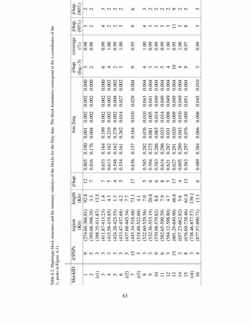
Tabl

e6.

2:H

aplo

type

bloc

kst

ruct

ures

and

the

sum

mar

yst

atis

tics

ofth

ebl

ocks

for

the

Dal

yda

ta.

The

bloc

kbo

unda

ries

corr

espo

ndto

the

x-co

ordi

nate

sof

the

λe

peak

sin

Figu

re6.

11.

bloc

kID

#SN

Psre

gion

leng

th#

hap.

Anc

.freq

#ha

p.co

vera

ge#

hap.

#ha

p.(K

b)(K

b)(f

rq>

3)(%

)(9

5%)

(90%

)1

9(2

74.0

4-36

6.81

)92

.812

0.80

50.

190

0.00

10.

002

0.00

20.

000

30.

983

22

5(3

95.0

8-39

8.35

)3.

37

0.81

60.

176

0.00

40.

002

0.00

20.

000

20.

982

2(r

1)3

(398

.35-

411.

87)

13.5

33

(411

.87-

413.

23)

1.4

70.

633

0.16

40.

199

0.00

20.

002

0.00

06

0.99

43

43

(415

.58-

419.

85)

4.3

50.

613

0.16

20.

219

0.00

20.

002

0.00

24

1.00

22

53

(424

.28-

425.

55)

1.3

40.

548

0.16

20.

278

0.00

20.

008

0.00

22

0.99

22

63

(433

.47-

437.

68)

4.2

50.

534

0.16

10.

262

0.01

40.

027

0.00

23

1.00

32

(r2)

5(4

37.6

8-44

5.34

)7.

77

15(4

45.3

4-51

8.48

)73

.117

0.63

60.

157

0.16

40.

010

0.02

90.

004

90.

959

6(r

3)5

(518

.48-

522.

60)

4.1

83

(522

.60-

529.

56)

7.0

50.

585

0.28

20.

076

0.01

00.

043

0.00

44

1.00

43

93

(532

.36-

553.

19)

20.8

60.

594

0.27

50.

081

0.00

50.

041

0.00

43

0.99

32

109

(570

.98-

579.

82)

8.8

60.

583

0.28

60.

065

0.01

40.

049

0.00

43

0.99

32

116

(582

.65-

590.

59)

7.9

80.

614

0.28

60.

033

0.01

40.

049

0.00

45

0.99

32

123

(594

.12-

598.

80)

4.7

50.

621

0.28

70.

031

0.00

80.

049

0.00

44

1.00

32

1315

(601

.29-

649.

90)

48.6

170.

627

0.29

10.

020

0.00

90.

049

0.00

410

0.95

119

143

(657

.23-

662.

82)

5.6

40.

605

0.28

90.

043

0.01

00.

049

0.00

44

1.00

32

158

(676

.69-

738.

46)

61.8

130.

563

0.29

70.

076

0.00

90.

051

0.00

49

0.97

85

(r4)

3(7

38.4

6-87

7.57

)13

9.1

164

(877

.57-

890.

71)

13.1

60.

489

0.38

40.

066

0.00

60.

045

0.01

03

0.99

33

63

6.5 DiscussionWe have proposed a new Bayesian method, Spectrum, for jointly modeling genetic recombi-nation with mutation and population structure. Under a pool of complete founder haplotypes,Spectrum describes the underlying genetic process of recombination and mutation explicitly interms of the association between founders and modern individuals. By incorporating a hiddenMarkov Dirichlet Process prior, which facilitates a well-defined transition process between in-finite ancestor spaces, the proposed method can efficiently infer a number of important geneticvariables such as recombination hotspots and ancestor patterns, jointly under a unified statisticalframework.

Our model provides a new way of representing a population structure in terms of an ancestralspectrum which shows the ancestral association composition of each modern individual chromo-some with the chromosomal ancestors. While the existing method based on admixture models(Falush et al., 2003) gives some degree of clear population label information, it is less informativein showing the population diversity or relationship between populations in the genetic history.In contrast, the Spectrum identifies the structure of sub-populations by considering the differentancestral association patterns among populations, in addition to displaying the diversity amongindividuals and populations, which yields a more informative representation for the populationstructure among shared ancestors across the populations.

Moreover, Spectrum allows us to recover the recombination events in each individual chro-mosome. Unlike other existing methods based on HMMs for recombination analysis whichassume fixed recombination sites for the population and consider block-wise ancestors, we pro-posed a full generative model for haplotype inheritance which explicitly models the individual-level genetic recombination and mutation along the chromosome. Note that the recombinationrate provided by Spectrum is defined with respect to the hypothetical founder pool and has notbeen modeled as a per-generation rate typically used in traditional recombination rate estimationmodels. Therefore, it is more suited for recombination hotspot analysis or for downstream ap-plications that can benefit from the recombination block-structures such as admixture analysis orassociation studies.

As of now, Spectrum does not intrinsically capture the heterogeneity of recombination ratesover loci, and the recombination rates are determined by the posterior distribution of recombina-tion events under a universal recombination rate, rather than directly by a maximum likelihoodestimation of site-specific recombination rates as in Li (2003). Also, we have not addressed theissues of threshold calculations and confidence measures of hotspot predictions as in Li (2003).These problems are of importance in various applications such as linkage-based quantitative trainlocus mapping and disease-gene mapping. One way of addressing these issues is to explicitlyintroduce more recombination states, for example, for both base-line recombination and hotspot-recombination, into the infinite HMM we proposed. Another possible extension to the existingmodel is to introduce priors for site-specific recombination rates for Bayesian inference.

64

Chapter 7

Robust estimation of local genetic ancestryin an admixed population

7.1 Introduction

The problem of inferring genetic ancestries in a population has been widely investigated for var-ious applications such as disease gene mapping and population history inference. For example,the inferred ancestry information has been used in correcting the confounding effect by popula-tion stratification in association studies (Price et al., 2006; Wang et al., 2010). The examination ofloci that have elevated probabilities of a specific ancestry has also given critical clues in selectingout potential causal variants of certain diseases in admixture mapping (Cheng et al., 2009, 2010;Zhu et al., 2011). Broadly, two different problem settings have been commonly considered forancestral structure analysis (Alexander et al., 2009), one on the ‘global ancestry’ that considersthe average proportion of each contributing population across the genome in an un-supervisedway (Alexander et al., 2009; Falush et al., 2003; Patterson et al., 2006); and the other on the ‘lo-cal ancestry’ that is more concerned with a locus-by-locus ancestry given reference populationdata (Pasaniuc et al., 2009; Price et al., 2009; Tang et al., 2006). We consider the problem ofestimating the local ancestry in an admixed population. A common scenario is to decompose thechromosomes of modern African Americans into blocks that have either African or Europeanancestry given the population data close to ancient African and European populations, which wecall ancestral populations. The populations of CEU and YRI are the most typical choices forsuch ancestral population data when an admixed population of African Americans is considered.We present a new haplotype-based method for local ancestry estimation that can deal with anarbitrary number of ancestral populations in a non-parametric Bayesian framework.

A natural approach to this problem involves a Hidden Markov Model (HMM) that tracesthe ancestry of each individual along the markers on a chromosome. A number of differentapproaches have been proposed and theses methods can be largely categorized into two fami-lies depending on how they represent the ancestral populations so that the local ancestry in anadmixed population can be estimated with respect to the reference information encoded by thepopulation representation method. The first family of methods use population-specific allele fre-quency profiles as reference information as in traditional admixture studies (Alexander et al.,

65

2009; Falush et al., 2003; Huelsenbeck and Andolfatto, 2007; Pritchard et al., 2000). Despite itssimplicity, low computational cost, and availability of such frequency profiles in representativedatasets, it is rather unnatural to model Linkage Disequilibrium (LD) under this setting becausethe correlations between loci are reflected only by the variation in such allele frequencies and notby the actual recombination events at the chromosome level. Therefore, either a subset of mark-ers in low LD has to be selected in a preprocessing step, or a recombination process often needsto be indirectly embedded to utilize a denser set of markers (Pasaniuc et al., 2009; Pattersonet al., 2004; Tang et al., 2006). The representation power of this family of methods thus tends todiminish when the correlations between markers are not carefully considered (Price et al., 2008).

Another family of methods are based on haplotype data that may contain richer informa-tion. These methods utilize representative haplotypes taken from each ancestral population dataas reference information for the local ancestry estimation (Price et al., 2009; Sundquist et al.,2008). Each haplotype in an ancestral population, which we call an ancestral haplotype, consti-tutes a hidden state in an HMM and the basic transition mechanism involves traversing amongthese ancestral haplotypes. Although these approaches provide a more natural way to reflect theunderlying admixing process by simulating recombinations at a real chromosome level, the in-ference result can be rather sensitive to the size and the choice of such ancestral haplotype data.Moreover, few existing methods make use of the genetic relatedness between ancestral popula-tions resultant from ancient population history and therefore the populations have been typicallytreated as independent. To improve the robustness and the accuracy in light of these issues, HAP-MIX (Price et al., 2009) introduces a ‘miscopying’ parameter that allows a small possibility foran allele to be copied from population 2 even when it is assumed to be originated from ancestralhaplotype in population 1. In this way, it prevents unnecessary transitions among ancestral popu-lations during inference and the allelic information in one population can be naturally borrowedby another population. However, this method is limited to two-way admixture that involves onlytwo ancestral populations, and it is not trivial to generalize this model to consider more generaldemographic scenarios.

We propose a new Bayesian approach for local ancestry estimation that utilizes the multi-population haplotype data in a more systematic way. Our method is built on the assumptionof a common pool of hypothetical founder haplotypes from which the ancestral haplotypes inmultiple ancestral populations are to be inherited, and from which in turn the individuals in anadmixed population are generated as well by the admixing process between ancestral popula-tions. Motivated by the population model described in Chapter 6 and in Sohn and Xing (2007b,2009), we represent the ancestral population data by an infinite hidden Markov model in whichthe hidden states correspond to the unknown number of hypothetical founder haplotypes. Therecombination and mutation events are then modeled with respect to these founders as transitionand emission process. For an individual in an admixed population, we extend the hidden statespace to a joint space of founder haplotypes and ancestral populations. That is, we incorporatea hidden state variable consisting of two indicator variables, one for selecting the hypotheti-cal founder haplotype and the other for selecting the ancestral population that it is originatedfrom. The hidden state variable corresponding to the ancestral population determines the localadmixing status and hence defines the local ancestry along the markers. Furthermore, population-specific time parameters are incorporated and scale the recombination rates in the correspondingpopulations accordingly to explain the gap between the hypothetical era of founder haplotypes

66

and each of the ancestral populations. We observe that this also enhances the robustness of ourmodel under scenarios that deviates from the common modeling assumption that all the popula-tions participate in the admixture simultaneously.

A subtle issue in the proposed representation is how to choose the number of founders andhow to construct them efficiently across multiple populations. Naıvely, we may assume Kfounders per population, but under this setting, not only one has to employ a non-trivial modelselection process to determine K, but also there is in general no correspondence between the Kfounders in one population and another set of K founders in a different population. This prob-lem would not only result in serious identifiability and multi-modality issue that can severelyslow down inference, but also, it will restrict the information sharing across populations andhence compromise the accuracy of ancestry estimation as well. On the other hand, if we are touse one shared set of K founders, the representational power of population-specific HMM canalso be limited. A non-parametric Bayesian framework using an infinite hidden Markov modelgives a natural solution for this (Beal et al., 2002; Teh et al., 2010). Under an infinite HMM,an unbounded number of founder haplotypes can be systematically handled to describe a studypopulation. If we employ multiple such infinite HMMs defined over the same set of founders,one infinite HMM per population, then it allows the founders to be shared between populations,while different populations do not have to include all these founders and can have a unique setof founders with its own frequency and recombination patterns among them. The number andthe haplotypes of the founders are recovered as a result of posterior inference from data. Un-der a Dirichlet process prior, the posterior typically yields a parsimonious set of founders. Thisnon-parametric Bayesian framework allows us to exploit the genetic relatedness between popu-lations in a principled way by describing the ancestral populations in terms of a common set offounder haplotypes. In Sohn and Xing (2009), a similar approach using a hierarchical Dirichletprocess has been successfully used for the problem of haplotype inference from multi-populationdata. However, the recombination process was not explicitly modeled in that work and a ratherheuristic approach was employed to handle the linkage disequilbrium structure.

The proposed approach is fully model-based and fundamentally different from conventionalhaplotype-based approaches that model genetic processes directly on the given haplotypes in theancestral population data. In our model, genetic processes such as recombination or mutationtake place with respect to the hypothetical founders, and not between the ancestral haplotypesand the admixed individuals. By basing our model on the hypothetical founders that lie on top ofand give rise to both ancestral and admixed population data, we utilize the multi-population dataand their relatedness efficiently, unlike most existing approaches that ignore such information.

In summery, the proposed model-based approach for ancestral inference enjoys enhanced ro-bustness and accuracy, evidenced by its substantially less sensitivity to the choice and the amountof ancestral population data comparing to other benchmark algorithms. In particular, our methodshows very competitive performance even when the sample size of the ancestral population datais very small. This highlights the potential usefulness of this method in the analysis involvingunderrepresented populations of limited data availability. In addition, the compact populationcharacterization by an infinite hidden Markov model improves the model flexility over existingapproaches so that it can naturally handle an arbitrary number of ancestral populations instead ofonly two, and can be easily generalized to cases with even more complex demographic scenarios.It is also robust even under deviation from the typical modeling assumption that multiple popu-

67

lations participate in the admixture at the same time. Our method can utilize the whole admixedpopulation data together to recover the model parameters such as the population proportion, orthe time-scaled recombination rate, while most existing approaches require those parameters asinput. The estimated parameters can reveal important clues on the history and the characteristicsof the study population as will be shown in our empirical data analysis.

7.2 The statistical model

7.2.1 Problem setting

We consider an admixed population in which J ancestral populations have mixed since G gen-erations ago. For example, if we are to recover the local ancestry of individuals in a Latinopopulation (admixed population), we can incorporate J = 3 populations of ancient African, Eu-ropean, and Native American as our ancestral populations. In our problem setting, we assumethat the haplotypes of single nucleotide polymorphisms are given for the ancestral populationsand the admixed population. We will recover the pool of hypothetical founder haplotypes andtheir associations to individuals by statistical inference. The association of admixed individualsto the ancestral populations will be recovered along with their association to the founders, whichwould lead to the estimation of local ancestry.

7.2.2 Overview of admixture model based on founder haplotypes

The choice of representation about how to characterize a population is the crucial starting pointin admixture modeling. Unlike most previous approaches that typically use allele frequency pro-files (Pasaniuc et al., 2009; Sankararaman et al., 2008a) or representative ancestral haplotypes intheir raw forms (Price et al., 2009; Sundquist et al., 2008), we employ a new haplotype-basedmethod that builds on an assumption of hypothetical founder haplotypes of unknown cardinality.The founder-based population model with explicit recombination modeling has been introducedin Sohn and Xing (2007b) with the application to population structure and recombination analy-sis. Under this approach, each individual in a population is generated from the hypothetical poolof founders via a series of recombination and mutation. An individual chromosome can then beviewed as a mosaic of the founders whose pattern is determined by the association with founders.This mosaic process could be modeled as a Hidden Markov model in which the founders corre-spond to the hidden states, the individual haplotypes correspond to the observation sequences,the transition process is modeled by the recombination process, and the emission process by themutation from founders to the individuals. By employing an infinite hidden Markov model, thenumber and the haplotypes of the founders can be recovered through posterior inference ratherthan being pre-specified; and the (local) inheritance association between the founders and thestudy individuals can also be derived.

Now we further extend this approach to model admixture events from an arbitrary numberof ancestral populations. When the ancestral populations start to mix and form an admixedpopulation, each individual chromosome in the admixed population can be decomposed intoblocks with distinct ancestry. For each of these blocks, we can trace back the source of the

68

11011000111010010100111100101011011010011011

Ancestral population 1

00010000000001010000110011101000101101000001

Ancestral population 2

11001010001

Admixed individual

Hypothetical Founders

T1 generations, , T2 generations

…

… …

…

G generations

11111112222 Local Ancestry…

Figure 7.1: Graphical illustration of the proposed model

genetic materials to a haplotype in the corresponding ancestral population. Now, recall that this‘ancestral haplotype’ is modeled as a mosaic of its founders. This means that each ancestry blockin an admixed individual is further dissected into a finer-grained mosaic of founders. Therefore,the admixed inheritance process is a composite process with two different resolutions, one fromthe founders to ancestral haplotypes, and the other from the ancestral haplotypes to the admixedindividuals. A graphical illustration of the proposed model is shown in Figure 7.1. A variant ofthe infinite hidden Markov model is employed to make the choice of founders and the ancestralpopulations at the same time along the chromosome.

7.2.3 Statistical model for generating ancestral and admixed populationdata

We now describe in detail the admixed inheritance model as a generative process of the individ-ual chromosomes in ancestral populations and an admixed population with respect to a set ofhypothetical founders.

Transition and emission probabilities

Our model involves a mosaic of two related jump processes of different genetic resolutions:recombination between founders, and admixture over ancestral populations. For ease of descrip-tion, we assume that the individuals are haploids. Let individual haplotypes be indexed by i,ancestral populations by j, and the markers by t. And let Hit ∈ {0, 1} and Akt ∈ {0, 1} repre-sent the allele of individual i and founder k at marker t, respectively. We introduce a set of hidden

69

state variables Sit = (Cit, Zit) where Cit ∈ {1, 2, ...} and Zit ∈ {1, ..., J} represent the indicatorvariables that select a founder and an ancestral population, respectively, on an i-th individualchromosome at marker t. For each ancestral population j, let νjk be the initial and backgroundprobability of founder k, and let πjk′k be the transition probability that determines the recombi-nation probability from founder k′ to founder k. To take into account the different strength andpattern of the recombination across different populations, we also introduce a set of time param-eters, Tj ∈ (0,∞), for each ancestral population j, such that Tj corresponds to the hypotheticaltime (generations) from the pool of founders to an ancestral population j. Similarly, G ∈ [0,∞)represents the time since admixture, that is, the time from ancestral populations to the admixedpopulation. Let η = (η1, ..., ηJ) denote the population proportion variable such that ηj is theexpected proportion of ancestral population j in an admixed population. r = (r1, r2, ...rT ) andd = (d1, . . . , dT ) represent the recombination rate and the physical distance between each neigh-boring markers, respectively. The final transition probabilities and the emission probabilities aredefined as follows:

P (Si,0 = (k, j)) = P (Zi,0 = j)P (Ci,0 = k) = νjkηj

P (Sit = (k, j) | Si,t−1 = (k′, j′)) = (1− e−rtdtG)νjkηj +

e−rtdtGe−rtdtTjδ(k = k′)δ(j = j′) +

e−rtdtG(1− e−rtdtTj)πjk′kδ(j = j′) (7.1)

P (Hit | Sit = (k, j), Akt) = θI(Hit 6=Akt)k (1− θk)I(Hit=Akt) (7.2)

We assume a founder-specific mutation parameter θk that determines the probability of mutationfrom a founder k to individuals.

The overall idea underlying this representation is the two-layered inheritance framework, onefrom the time of hypothetical founders to ancestral populations, and the other from those ances-tral populations to the admixed population. If we set G = 0 in Equation (7.1), this two-layeredframework is reduced to the model of the first layer that characterizes the ancestral populationswith respect to the founder haplotypes. Under the reduced model, each population is associatedwith its own hidden Markov model parameters and the recombination rate scaled by Tj . Suppose(Ci,t−1, Zi,t−1) = (k′, j′) which means i-th chromosome has inherited from founder k′ at markert− 1 in ancestral population j′. At the next marker t, it either selects a new founder k with prob-ability (1 − e−Tjrtdt)πjk′,k and set Cit = k, or no recombination takes place with the remainingprobability and Cit = Ci,t−1. If we trace the values of Cit across all the t, it will decompose thechromosome i into blocks with distinct associated founders. Therefore, each chromosome canbe thought of as a mosaic of such founders.

Now, at the second layer which involves the admixture, this sequential process for selectingfounders Cit occurs within the same ancestral population with probability e−rtdtG so that Zit =Zi,t−1. Or with probability (1 − e−rtdtG), a new population j as well as a new founder k ischosen jointly with a probability proportional to the product of population proportion ηj and thebackground probability νjk. Therefore, chromosomes both in the ancestral populations and in theadmixed population are modeled as mosaics of founders determined by the sequence of Cit. Inaddition, each admixed individual i is associated with another resolution of mosaic determinedby the sequence of Zit across t. The estimation of local ancestry can be done by tracing theposterior probability of Zit along the markers.

70

Note that even when no admixture is assumed, we still have the flexibility of choosing adifferent founder chromosome. This feature helps to control the number of transitions amongpopulations effectively so that the hidden state doesn’t need to change excessively. Moreover,the population-specific time parameters scale the recombination probabilities accordingly so thatmore ancient populations can have higher probabilities of recombination with respect to thefounders. This representation is especially useful in producing heterogenous resolution of mo-saics in different ancestral populations. Although we assume the J populations participate in theadmixture simultaneously, those parameters allow various resolution of recombination patternsin ancestral haplotypes and this greatly improves robustness of the model against the violationsof such modeling assumption as well as the accuracy of the ancestry estimation.

The cardinality of the founder space

Instead of fixing the number of hypothetical founders by doing statistical model selection, weadapt a more flexible non-parametric approach by employing an infinite hidden Markov model(Beal et al., 2002; Teh et al., 2010) so that the number of hidden states does not need to be pre-specified. Recall that if we consider a finite, say K, hidden states, the transition probabilitieswill be represented as a K × K matrix. Each row k of this matrix sums to one and defines theprobabilities of switching from a source state k to all the target states.

Now, if we consider an infinite hidden state space, each row of the transition matrix would bean infinite dimensional vector which sums to one and the Dirichlet Process (DP) (Blackwell andMacQueen, 1973; Ferguson, 1973) has been effectively used to describe such probability distri-butions. To ensure all the row-specific DPs are built on the same state space, another DirichletProcess is shared as a common base measure at a top level, which actually corresponds to a hi-erarchical Dirichlet Process model (Teh et al., 2010). Basically, (k, k′)-element of the transitionmatrix πj defines the transition probability from state k to state k′ in population j, and for agiven source state k, the target state index k′ can increase as large as needed by the given data.Infinite-dimensional vector of initial probabilities νj can be defined in a similar way under thesame hierarchical Dirichlet process framework. Since we consider multiple such infinite HMMsfor multiple populations, we let the same base measure shared across all the populations. Thisinfinite HMM-based framework leads to a very simple solution to how many founders to con-sider and how to construct the founder space across multiple populations. The HMM parametersof our admixture model thus can be summarized as follows:

β ∼ GEM(γ)

νj ∼ DP (τ, β)

πjk ∼ DP (τ, β)

where τ and γ define the scale parameters for the population-specific DPs and the top level DP,respectively.

Other parameter description

We assume Beta prior for each of the mutation parameters θk, and Dirichlet distribution prior forthe population proportion parameter η ∼ Dirichlet(ξ1, ..., ξJ).

71

For simplicity of inference, we transform the variables such that rt and Tj are combined asgrjt = rtTj . Similarly, we use the notation Gr

t := rtG. We assume these variables are i.i.d underGamma prior. Then Equation (7.1) is transformed as follows:

P (Sit = (k, j) | Si,t−1 = (k′, j′)) = e−Grt dte−g

rjtdtδ(k = k′)δ(j = j′) +

e−Grt dt(1− e−grjtdt)δ(j = j′)πjk′k +

(1− e−Grt dt)νjkηij (7.3)

In summary, infinite hidden Markov model parameters combined with population geneticsparameters are used to capture different characteristics in populations and to describe admixtureevent from an arbitrary number of populations in a unified framework. While we assume aninfinite number of founders a priori, the posterior inference usually produces a small number offounders and this gives a compact representation of populations for the admixture analysis.

7.2.4 Posterior Inference

To overcome the drawbacks of slow convergence in traditional Gibbs sampling, we employ avariant of beam sampling proposed for infinite HMMs (Van Gael et al., 2008). Basically, itextends the well-known dynamic programming technique of the forward-backward algorithm ina finite state HMM to an infinite state space case. It exploits the property that in an observationsequence of finite length, the number of actually realized hidden states is finite at each iterationstep. Therefore, the number of states to be considered in forward-backward algorithm can beadaptively changed over iterations.

Forward-backward algorithm for the proposed infinite HMM

We introduce auxiliary variables ut for t = 0, ..., T − 1 with the following distribution:

ui0 | Si0 = (k, j) ∼ Uniform(0, νjkηij)

uit | Sit = (k, j), Si,t−1 = (k′, j′) ∼ Uniform(0, qit) for t = 1, ..., T − 1

where

qit = e−Grt dte−g

rjtdtδ(k = k′)δ(j = j′) +

e−Grt dt(1− e−grjtdt)δ(j = j′)πjk′k + (1− e−Grt dt)νjkηj

For notational convenience, we omit the notation i. Let the forward probabilities be

αt(k, j) = P (St = (k, j) | H0:t, u0:t)

72

Then

α0(k, j) ∝ P (S0 = (k, j), H0, u0) ∝ P (S0 = (k, j))P (u0 | S0 = (k, j))P (H0 | C0 = k)

= δ(u0 < νjkηZ0)P (H0 | C0 = k)

αt(k, j) ∝∑k′,j′

P (St = (k, j), St−1 = (k′, j′), Ht, ut | H0:t−1, u0:t−1)

∝ P (Ht | Ct = k)∑k′,j′

P (ut | St = (k, j), St−1 = (k′, j′))×

P (St = (k, j) | St−1 = (k′, j′))αt−1(k′, j′)

∝ P (Ht | Ct = k)×J−1∑j′=0

∞∑k′=0

δ(ut < P (St = (k, j) | St−1 = (k′, j′)))αt−1(k′, j′) (7.4)

Given u0, ..., uT−1, the number of states k such that αt(k, j) > 0 for t = 0, ..., T − 1 is finite: fort = 0, the number of k such that νjk > u0 is finite for any j since

∑k νjk = 1 with νjk ≥ 0, and

recursively, we can see the number of k with αt(k, j) > 0 is finite. Therefore, the infinite sumover the previous states in the calculation of forward probability reduces to a finite sum.

CT−1 and ZT−1 can be sampled from αT−1(k, j). Then for t = T − 2, ..., 0, we sample Ctand Zt using

P (Ct, Zt | H0:T−1, u0:T−1, Ct+1, Zt+1) ∝P (Ct+1, Zt+1 | Ct, Zt)αt(Ct, Zt)P (ut+1 | St, St+1)

Since the entire inheritance process from founders to ancestral populations and then the ad-mixed population is modeled in a single Bayesian framework, it allows the exact posterior in-ference by putting the ancestral and admixed population data together in a single series of beamsampling iterations described above. However, this is not optimal in terms of time complexityas we often favor to run multiple test sets after we get reference information about the ancestralpopulations. Therefore, we split the whole inference process into two phases: 1) training phasewhere the model parameters about ancestral populations are learned, and 2) ancestry estimationphase that actually recovers the ancestry of admixed individuals.

One caveat of this decomposition is that we may not fully take advantage of the flexibilityof the infinite model. This is because we need to constrain the hidden state space somehow asa finite space when the output from the training phase is returned. As an n-th posterior samplefrom Bayesian inference of the training phase, we get a finite numberK(n) of founder haplotypesand the related HMM parameters of π(n) and ν(n) with gr(n)

j for each j. Averaging these results asone training output is not straightforward as K(n) can be different across different n. A plausibleapproach would be to keep multiple, say N posterior samples S = {A(n), π(n), ν(n)}n=1,...,N andrun the ancestry estimation routine N times using each of these parameters in S. Then the Nposterior distributions of the ancestry indicator variable Z can be easily averaged to form thefinal posterior distribution since Z is defined over a fixed number of populations J unlike C orother parameters that depend on K. Note that gr(n)

j does not depend on K, so we can use the

73

posterior mean of gr(n)j as the final estimate for it. Another practical approach would be to select

a single output from the training phase such as a MAP solution, and estimate the local ancestrybased on the single set of parameters. Empirically, we observe that the performance degradationby this MAP solution with respect to the first approach is relatively small.

Training phase

For an individual in an ancestral population j, we can set the time since admixture G to bezero and the population indicator variables Z to be observed as constant. Then the hidden statevariable Sit = (Cit, Zit) can be replaced with a Cit indicating the founder and Equation (7.3) isreduced to the followings :

P (Ci0 = k) = νZi0k

P (Cit = k | Ci,t−1 = k′) = e−grZi0t

dtδ(k = k′) + (1− e−grZi0t

dt)πZi0k′k

We infer the variable C through the Beam sampling algorithm, and the other variables throughthe standard Gibbs sampling. If we reduce the model to the training phase, we can treat thevariable Z as observed. Therefore, the forward probabilities are written as follows:

α0(k) ∝ P (C0 = k,H0, u0) ∝ P (C0 = k)P (u0 | C0 = k)P (H0 | C0 = k)

= δ(u0 < νZ0kηj)P (H0 | C0 = k)

αt(k) ∝∑k′

P (Ct = k, Ct−1 = k′, Ht, ut | H0:t−1, u0:t−1)

∝ P (Ht | Ct = k)∑k′

P (ut | Ct = k, Ct−1 = k′)P (Ct = k | Ct−1 = k′)αt−1(k′)

∝ P (Ht | Ct = k)∞∑k′=0

δ(ut < P (Ct = k | Ct−1 = k′))αt−1(k′) (7.5)

Note that the contribution of transition at each neighboring loci t − 1 and t to the pa-rameter π and grjt is not all equal because of the self-transition probability forced by the re-combination model in Equation (7.3). We handle this by sampling auxiliary binary variablesMit ∼ Bernoulli(1− e−g

rZi0t

dt) to indicate whether the jump occurs in the transition or not. Thetransition probability can be decomposed as follows:

P (Cit | Ci,t−1) = P (Mit = 0)δ(Cit = Ci,t−1) + P (Mit = 1)πjCi,t−1,Cit

Then we sample Mit given Cit and Ci,t−1 backward in forward-backward process from

P (Mit|Cit = (k, j), Ci,t−1) ∝ P (Mit)P (Cit = k | Ci,t−1 = k′,Mit)

Now, π can be sampled as in Van Gael et al. (2008), but conditional on M , which involvesthe transitions with Mit = 1 only. grjt can also be sampled conditional on M using P (grjt |{C:t, C:,t−1,M:t}) ∝ P (grjt)

∏i∈Pop j P (Ci,t | Ci,t−1,Mit). The overall sampling procedure is

summarized in Algorithm 1.

74

Algorithm 1 Procedure for training iHMMs in reference populationsInput: Haplotype data H for ancestral populationsOutput: N posterior samples of founders and the related HMM parameters{A(n), π(n), ν(n),gr(n)} for n = 1, . . . , N

1: repeat2: for each individual chromosome i do3: Sample the auxiliary variables uit for t = 0, ..., T − 1.4: Sample Cit | u,H,A using the beam sampling algorithm5: Sample Ak,t and θk6: Sample parameters ν, π, β and gr.7: end for8: until convergence

Algorithm 2 Procedure for estimating local ancestry in an admixed individualInput: Haplotype data H for an admixed population, estimated parameters{A(n), π(n), ν(n),gr(n)}Output: Posterior distribution of Z = (Zit) .

1: for n = 1, . . . , N do2: repeat3: for each individual chromosome i do4: Sample Sit = (Cit, Zit) | H,A using the forward-backward algorithm5: Sample θ, η, and Gr .6: end for7: until convergence8: Keep S posterior samples of Z9: end for

10: Average N · S posterior samples and return the final posterior distribution of Z

Ancestry estimation phase

As the variables A, gr, ν, π are returned in the training stage, the unknown variables now are theadmixture proportion η, the generations since admixture G, the mutation rate θ of founders, andS = (C,Z) for the admixed individuals. We re-sample θ in the ancestry estimation phase insteadof getting it from the training step because θ can reflect additional information about the admixedpopulation by describing it in terms of the discrepancy between founders and the population.As we now deal with a finite number of hidden states obtained from the training phase, it isnot necessary to incorporate the auxiliary variable u to sample S in the ancestry estimationphase. The variables Sit thus are sampled through a standard forward-backward algorithm. Asin the training stage, the transition probability at each marker can be decomposed into two parts,depending on whether the jump process for admixture occurs or not. We use the similar techniqueto sample Gr by introducing an auxiliary variable Lit ∼ Bernoulli(1 − e−G

rt dt). The overall

sampling scheme is summarized in Algorithm 2.If the time since admixture G, population proportion η, and the recombination rate r is as-

75

sumed to be known as is often the case in typical admixture analysis, we can omit the second stepof parameter sampling (line 5 in Algorithm 2) and re-use θ that can be returned from the trainingstage. Then it is also possible to get an approximate solution by use of a posterior decoding fromforward-backward steps in a finite dimensional HMM.

7.3 Result

7.3.1 Simulation designTo validate the proposed method, we simulated admixed individuals using Human Genome Di-versity Project (HGDP) data genotyped on Illumina Infinium HumanHap550 BeadChips (Jakob-sson et al., 2008). Considering previous results that have revealed distinct genetic characteristicsacross different continents, we selected reference populations that would serve as putative an-cestral populations: YRI for African ancestry, CEU for European, JPT and CHB for East Asia,and Maya for Native American ancestry. Each of the resulting ancestral populations contained30, 30, 28, and 13 individuals, respectively. We first focus on chromosome 22 in the simulationstudy.

To take into account the discrepancy between real ancestral populations and those used intraining, we generated admixed individuals using populations which are similar but not identicalto those used as ancestral populations. For example, individuals in Russian and BantuKenyapopulations are mixed to simulate an admixed population and then the local ancestries of theseindividuals are estimated with respect to CEU (European) and YRI (African) populations. Foreach simulation scenario below, we generate 30 admixed individuals.

The performance is measured as the mean squared error rate of ancestry probabilities alongthe loci. Specifically, let pijt denote the probability of ancestry j at a locus t in an individuali. The average error rate of

∑Jj=1

∑Tt=1(ptrueijt − pestijt )2/T across all the individuals is reported.

We compare our results with the two state-of-the-art methods that stem from different populationrepresentation methods : LAMP (Pasaniuc et al., 2009; Sankararaman et al., 2008b), the methodbased on allele frequency profiles as reference information, and HAPMIX (Price et al., 2009)that uses representative individual haplotypes in the ancestral populations, which appear to out-perform other available methods such as HAPPA (Sundquist et al., 2008), SABER (Tang et al.,2006) or ANCESTRYMAP (Patterson et al., 2004) from previous studies. Since these benchmarkalgorithms require the parameters for recombination r, the admixture time G, and the populationproportion η to be specified as input, we provided the true values of these parameters to all thealgorithms in the simulation study. Additionally, each haplotype data for ancestral populationswere converted to allele frequency profiles and then LAMP was run with these frequency data asinput. For the analysis below, we used the MAP solution as our parameter estimation from thetraining phase.

7.3.2 Performance on two-way admixtureThe first simulation scenario considers two-way admixture of ancient European and Africanpopulations. The proportion of each ancestral population was set to be equal (η = (0.5, 0.5)).

76

True

FDhap

HAPMIX

LAMP

Figure 7.2: True and estimated local ancestries of two sample individuals in an admixed population from Africanand European populations. The x-axis corresponds to chromosomal position and the y-axis corresponds to theancestry probability (yellow: African, dark grean: European)

The local ancestries of the admixed individuals were estimated based on the trained model usingtwo ancestral populations of African (YRI) and European (CEU). In Figure 7.2, we first displaythe true and the estimated local ancestry probabilities of two sample individuals in an admixedpopulation. The yellow color corresponds to African ancestry, and the dark green corresponds toEuropean ancestry. The length of the vertical color bar at each chromosomal location along thex-axis is proportional to the corresponding ancestry probability. While all the algorithms producereasonable results in general, the proposed method denoted by FDhap (FounDer haplotype basedadmixture model) is especially effective in picking out fine details of ancestry changes as can beseen in the example.

The overall performance of each algorithm across all the generated samples are shown inFigure 7.3. Roughly, we can see that FDhap and HAPMIX perform comparably to each otherand tend to outperform LAMP. Still, all the three algorithms perform reasonably well as canbe seen in the small overall error rates. For example, the average error rates for G = 10 were0.0077, 0.0086, and 0.0116 in FDhap, LAMP, and HAPMIX, respectively.

7.3.3 Performance as a function of data size in training setTo further evaluate each method in terms of its performance with respect to the training datasize, we varied the number of available individual samples per ancestral population. Specifically,we trained the model using 3, 5, 10, 20, 30 individuals, hence, 6, 10, 20 40, 60 haplotypes, perancestral population and estimated the ancestries based on each of the trained model. The sametwo-way admixture scenario from African and European populations is considered of which theresult on the full dataset is shown in Figure 7.3. The performance of each algorithm is presentedas a function of training data size in Figure 7.4. It is clearly seen that the proposed methodsubstantially outperforms the other benchmark algorithms, especially when the data size is small.Even when only a few ancestral haplotypes are available, it still gives very good estimates of the

77

FDhap hapmix lamp0

0.01

0.02

0.03

0.04

err

FDhap hapmix lamp0

0.01

0.02

0.03

0.04

err

FDhap hapmix lamp0

0.01

0.02

0.03

0.04

0.05

0.06

err

(a) (b) (c)

Figure 7.3: Boxplot for mean squared error rates of ancestry estimation for two-way admixture of African andEuropean populations since G generations ago with (a)G = 5, (b) G = 10, and (c) G = 20.

3 5 10 20 300

0.02

0.04

0.06

0.08

# Individual per ancestral population

err

FDhaphapmixlamp

3 5 10 20 300

0.02

0.04

0.06

0.08


err

FDhaphapmixlamp

3 5 10 20 300

0.02

0.04

0.06

0.08


err

FDhaphapmixlamp

(a) (b) (c)

Figure 7.4: Error rate as a function of the number of individuals per train population. Two-way admixture of Africanand European popualtions since G generations ago with (a) G = 5, (b) G = 10, and (c) G = 20.

local ancestries compared to the others. Therefore, our method can be especially useful in theanalysis of admixture effect involving non-traditional populations where the amount of availablegenotypes is still limited.

7.3.4 Performance on three-way admixture

We now consider the admixture that involves more than two ancestral populations. Analogousto the formation of Puerto Rican population (Tang et al., 2007), we included CEU, YRI, andMaya populations as ancestral populations for African, European, and Native American ances-try, and generated an admixed population using Russian, BantuKenya, and Pima with admixingproportion of 0.66, 0.18, and 0.16, respectively. Figure 7.5 shows the resulting error rates acrossdifferent values of G. Since HAPMIX cannot handle more than two ancestral populations di-rectly, we ran it in three different modes such that each run tries to estimate the targeted ancestryversus the other two ancestries as was done its original paper (Price et al., 2009). For this rea-son, we compare the performance on each ancestry separately. Overall, our method performssignificantly better than the other two in most of the analyzed cases.

78

Afr

FDhaphapmix lamp0

0.05

0.1

err

FDhaphapmix lamp0

0.05

0.1

err

FDhaphapmix lamp0

0.05

0.1

err

Eur

FDhaphapmix lamp0

0.05

0.1

err

FDhaphapmix lamp0

0.05

0.1

err

FDhaphapmix lamp0

0.05

0.1

err

Nat

FDhaphapmix lamp0

0.05

0.1

err

FDhaphapmix lamp0

0.05

0.1

err

FDhaphapmix lamp0

0.05

0.1

err

G = 5 G = 10 G = 20

Figure 7.5: Boxplot for mean squared error rates of ancestry estimation. Three-way admixture of African, European,and Native American populations sinceG generations ago. Since HAPMIX is applicable to only two-way admixturecase and was run to estimate each ancestry versus the other two, we report the error rate on each ancestry separately.

79

0 0.2 0.5 10

0.02

0.04

0.06

0.08

err

G1/G20 0.2 0.5 10

0.02

0.04

0.06

0.08

err

G1/G20 0.2 0.5 10

0.02

0.04

0.06

0.08

err

G1/G2FDhap HAPMIX LAMP

Figure 7.6: Robustness under deviation from the modeling assumption. The x-axis represents the ratio G1/G2,where G1 denotes the number of generations for which the first two populations had mixed and G2 means theadditional number of generations since the third population joined and have further mixed together.

7.3.5 Robustness under deviation from admixture assumption

We investigate the robustness under deviation from the modeling assumption that all the ancestralpopulations participate in the admixing simultaneously. We generated admixed populations fromthree ancestral populations that started to mix at two different time points. More specifically,Russian and BantuKenya populations are mixed for G1 generations with 50%/50% proportion.Then this admixed population is mixed with the third population of Pima for G2 generationswith 50%/50%, resulting in the overall proportion of 0.5, 0.25, 0.25. We fixed G2 to be 10 andvaried G1 to be 0, 2, 5, and 10 where G1 = 0 corresponds to the case in which the modelingassumption holds. The result is summarized in Figure 7.6. In each plot for each algorithm, x-axis corresponds to the values of G1/G2 and y-axis shows the error rates. The proposed methodresulted in not only the lowest error rates, but also the most stable performance across differentvalues ofG1/G2. For more quantitative comparison of robustness across different algorithms, wecalculated the linear regression coefficient of G1/G2 versus the error rates. The resulting slopeswere -0.0011, 0.0029, and 0.0074 for FDhap, HAPMIX, and LAMP, which again supports thesuperior robustness of the proposed method.

7.3.6 Sensitivity analysis on model parameters

Since the parameters of η and G were assumed to be known in our simulation study in parallelwith other methods, we also examine how the performance of FDhap is affected by incorrectlyspecifying these parameters. The performance is shown for the dataset simulated with G = 10and η = (0.5, 0.5) in Figure 7.7. In each plot, x-axis shows the specified parameters wherethe values are shown in log scale in case of G. We could see that there was almost no effectwhen η was incorrectly set in the range from 0.2 to 0.8. When we examined the result on G, thealgorithm had the general tendency to favor a specified value G smaller than the true value. Theeffect of mis-specified value of G was minimal when the discrepancy was within a factor of 2.Even in the extreme case such as G varied by a factor of 5, the error still remained within thetwice of the error rates when the true value was given.

80

2 3 4 5 6 7 80

0.01

0.02

0.03

η1

err

1 5 10 20 50

0.01

0.02

0.03

G

err

Figure 7.7: Sensitivity analysis: boxplot for error rates as a function of specified parameter values (a) η1 and (b) Gwhen the true values are ηtrue = (0.5, 0.5), Gtrue = 10.

7.3.7 Empirical analysis of HGDP data

To illustrate our method on real data, we applied it to 22 autosomes of the HGDP dataset (Jakob-sson et al., 2008). Four ancestral populations of YRI, CEU, JPT+CHB, and Maya were chosenas in the simulation study to represent African, European, East Asian, and Native American an-cestries. We then recovered the local ancestries in the remaining 28 populations. Since the timesince admixture is not available for real data, we let our program estimate the parameters byposterior inference.

The mean ancestry proportion of each population estimated from our algorithm is summa-rized in Table 7.1. Overall, the ancestry vector agrees very well with their geographical locationsor known history. For example, populations such as Yoruba, Mandenka, BiakaPygmy, or Bantu-SouthAfrica recovered pure African ancestries, Druze, Basque, Russian and Adygei populationshad dominant European ancestries (≥ 0.978), and Pima or Colombian populations resulted inalmost pure Native American ancestries (≥ 0.983).

More interestingly, the result also identifies the populations that have strong evidence ofadmixing effect among multiple ancestries. For instance, the proportion of European ancestry inUygur population was 0.35, that of East Asian ancestry was 0.41, and the remaining proportionof 0.24 in Native American ancestry. Previous analysis in Xu et al. (2008) and Xu and Jin(2008) claimed that Uygur had roughly 50–60% of European ancestry and 40–50% of East Asianancestry from the analysis based on two-way admixture. More recent study in Li et al. (2009)showed evidences that the estimation of European ancestry in these studies appear to be biasedand suggested a newly estimated proportion of around 30%. Our result largely agrees with theseresults in that the estimated East Asian ancestry (41%) is similar to that in Xu et al. (2008) and inaddition the estimation of European ancestry (35%) is closer to the more recent result in Li et al.(2009) than Xu et al. (2008). Considering its geographical location and the resulting populationhistory, we suggest that Uygur population has about 35% of European ancestry, 41% of EastAsian ancestry, and the remaining proportions of ancestries in other contributing populations thathave greater similarity to the Native American population. Although only one or two populationsare selected to serve as each putative ancestral population in our study, these populations have

81

Table 7.1: Estimated ancestry proportions of populations in HGDP dataset with respect to four ancestral populationsof African, European, East Asian, and Native American.

African European East Asian Native AmerYoruba 1.000 0.000 0.000 0.000Mandenka 1.000 0.000 0.000 0.000BiakaPygmy 1.000 0.000 0.000 0.000BantuSouthAfrica 1.000 0.000 0.000 0.000San 0.999 0.001 0.000 0.000MbutiPygmy 0.999 0.000 0.000 0.001BantuKenya 0.998 0.001 0.000 0.000Mozabite 0.141 0.818 0.013 0.028Bedouin 0.035 0.941 0.006 0.018Palestinian 0.013 0.966 0.006 0.015Basque 0.000 0.998 0.000 0.001Russian 0.000 0.990 0.003 0.007Druze 0.002 0.989 0.002 0.006Adygei 0.000 0.978 0.008 0.014Kalash 0.000 0.930 0.027 0.043Balochi 0.015 0.888 0.031 0.066Burusho 0.000 0.741 0.088 0.170Uygur 0.000 0.348 0.414 0.239Yakut 0.000 0.045 0.848 0.106Mongola 0.000 0.006 0.960 0.034Daur 0.000 0.004 0.972 0.024Cambodian 0.000 0.004 0.977 0.019Lahu 0.000 0.000 0.987 0.013Yi 0.000 0.001 0.991 0.009Melanesian 0.001 0.039 0.821 0.140Papuan 0.002 0.081 0.733 0.185Pima 0.001 0.012 0.004 0.983Colombian 0.002 0.001 0.001 0.996

82

shown to be close surrogates of the distinct ancestral components in a large number of studiesso far. Since our result is obtained by utilizing a denser set of markers as well, we believe ourestimates reveal more meaningful admixture proportions than the previous analyses.

To further analyze each population data, we examined the estimated parameters of Gr, theadmixture time scaled by the recombination rate, and the empirical mutation parameter θ com-puted as an average discrepancy between individuals and corresponding founders within each ofthe populations. Note that we can think of Gr as showing the relative strength of admixing effectin the population. Moreover, θ can be interpreted as the relative age of the population becauseit describes the gap between the common founders to the population. The result is displayed inFigure 7.8. We colored the bars based on the geographic location of the corresponding popula-tion. The result has nice correspondence with the known geographic labels as well. For example,all the populations in African continent showed the smallest values of Gr, indicating the lowestlevels of admixing effect. The top three populations suggesting the strongest admixing effectinclude Mozabite, Uygur, and Burusho. Most populations in the continents of East Asia andAmerica showed medium levels of admixing effect.

The empirical θ estimated for the data reveals more striking pattern. We find that the orderingof populations by their parameter values almost exactly agrees with the geographic locations outof Africa. That is, all the populations in African continent had the largest values of θ implyingtheir oldest ages, populations in Eurasia came next, and Oceanian populations were the third.Populations in East Asian region formed the fourth cluster and then Pima and Colombian pop-ulations showed the smallest values of θ which implies later formation of the populations thanothers. It is noteworthy that Yoruba, which appears to be the closest to the training populationof YRI, recovers a much larger value of mutation rate θ than all the populations in geographiclocations other than African continent. This comes from the nice property of our model that wedo not directly use the training haplotype data as our reference, we rather infer the correspondingcommon founders across all the population data together and then work in a framework dealingwith founders and admixed individuals. Otherwise, it would be impossible to obtain such a resultbecause the discrepancy of Yoruba and its reference data would be much smaller than most ofthe other populations.

Based on the analysis above, we selected 11 populations that showed elevated signals ofadmixture and show their local ancestry proportions in Figure 7.9 that can be used for furtherdownstream analysis.

7.4 DiscussionWe have proposed a new haplotype-based framework for modeling the admixing events over an-cestral populations and estimating the local ancestries of the individuals in the admixed popula-tion. By modeling hypothetical founders and their inheritance processes, and by using population-specific hidden Markov models to represent the ancestral populations with an unbounded numberof founders, our method can lead to accurate stratification of local ancestry of individual chro-mosomes in an admixed population.

Previous admixture studies have suggested that the world populations are not independentof each other, but rather are structured through population admixing history and the resulting

83

0 0.5 1 1.5 2x 10−8

YorubaBantuSouthAfrica

BiakaPygmyMandenka

SanBantuKenyaMbutiPygmy

YiBasque

LahuColombian

DaurRussian

CambodianPima

DruzeMongola

AdygeiPalestinian

YakutKalash

BedouinMelanesian

BalochiPapuan

BurushoUygur

Mozabite

estimated Gr

AfricaEurasiaEast AsiaOceaniaAmerica

0 0.005 0.01 0.015 0.02 0.025 0.03 0.035 0.04Colombian

PimaDaur

YiMongola

LahuYakut

CambodianUygur

MelanesianPapuanRussianBurusho

KalashBasqueAdygeiBalochi

DruzePalestinian

BedouinMozabite

YorubaMandenka

BantuKenyaBantuSouthAfrica

BiakaPygmyMbutiPygmy

San

estimated θ

AfricaEurasiaEast AsiaOceaniaAmerica

Figure 7.8: Estimated parameters sorted in decreasing order. Top: estimated Gr, time since admixture scaled byrecombination rate. Bottom: empirical mutation rate θ computed as the average discrepancy between individualsand their founders.

84

AfricanEuropeanEast AsianNative Amer

Mozabite

Uygur

Yakut

Mongola

Daur

Yi

Cambodian

Lahu

Melanesian

Papuan

Colombian

Figure 7.9: Map of ancestry proportions along chromosome 22 on admixed populations from HGDP data. The x-axis corresponds to chromosome positions and the y-axis denotes the ancestry proportion. We selected 11 admixedpopulations based on the estimated ancestry proportions such that the largest ancestry proportion is less than 90%

85

gene flow. Most existing approaches for local ancestry estimation have ignored such relatednessand treated the populations as unrelated. We explore this dependency among populations andefficiently utilize it by building a unified model that covers all the ancestral populations andthe admixed population together. As shown in our Results, this modeling strategy is especiallyhelpful when only a limited amount of data is available to represent the ancestral populations.Since genetic information in one population can be naturally shared by another population in sucha framework, it effectively enhances the robustness of the proposed model regarding the choiceof the ancestral population data. We expect that various types of practical analysis dealing withnon-typical study populations would benefit from the proposed method.

In our comparative study, HAPMIX appears to perform very well when enough data for an-cestral populations are given and also for older admixture events. However, this method doesnot allow one to analyze the admixing effect from more than two ancestral populations. Instead,one ancestry versus all the other ancestries should be estimated. While this setting may be finefor some applications, this constraint limits its applicability to complex admixture scenarios andmay compromise its ability to deal with older admixtures. LAMP has a slightly different focus:while its performance was shown to be worse than the other two in general in our simulationstudy, it can deal with multiple ancestral populations as our model. And computationally thismethod was significantly faster than the other two haplotype-based methods. However, LAMPseems to be more suited for very recent admixture case, and its performance tends to drop quitesharply as we consider more ancient admixture events. On the other hand, in a very recent ad-mixture case, LAMP tends to be less sensitive to the amount of training data than HAPMIX asshown in Figure 7.4. Our approach is more general and of more practical utility in that it can in-corporate an arbitrary number of ancestral populations with comparable or superior performancethan HAPMIX under various scenarios. In comparison of computation time with HAPMIX, ourmethod requires additional, but off-line computation time for model training, which is linear inthe number of individuals and the number of markers. For the ancestry estimation phase, wewould additionally need a series of MCMC iteration times if we want to estimate the parametersof interest such as admixture time or mutation rates.

It is worth mentioning some of previous approaches for global ancestry analysis as wellto position our method in context. STRUCTURE (Pritchard et al., 2000) has been one of themost widely used softwares for admixture analysis, and more recently, other softwares such asEIGENSTRAT (Patterson et al., 2006) and ADMIXTURE (Alexander et al., 2009) have also gaingreat popularity especially for their computational efficiency. In global ancestry estimation prob-lems, typically no prior information is provided for the ancestral populations and the ancestriesof given individuals are recovered as mean proportions of each possible ancestry. Therefore, itcan be considered as an unsupervised problem. In contrast, local ancestries are mostly estimatedbased on the given reference information such as allele frequencies or genotypes of putative an-cestral populations. There has been more recent work that bridges the gap between these twoapproaches. For example, LAMP can also run in an ‘unsupervised mode’ such that it recoversthe allele frequency profiles of ancestral populations as well as the local ancestries. Also, AD-MIXTURE, which is for the global ancestry estimation, recently added a new feature that theknown ancestries of some reference individuals can be exploited (Alexander and Lange, 2011).For haplotype-based approaches, this extension is not straightforward in general because oneneeds to deal with a set of hidden haplotypes that results in a large number of parameters. Re-

86

garding this aspect, our model for the local ancestry has the desirable property that it integratesout the ancestral population data during the inference and works with the hypothetical foundersand the admixed population data. Therefore, we expect that the extension of the model to anunsupervised case would also be a promising direction to pursue.

In this approach, we assumed that phased haplotype data are given. In practice, a number ofsoftwares are available for haplotype phasing (Browning and Browning, 2009; Li et al., 2010;Scheet and Stephens, 2006), so the phase information can be readily available in processingstep. It would also be quite easy to extend the model to deal with unphased genotypes. Forexample, we may assume that the haplotypes of ancestral populations are given, and then weallow unphased genotypes for admixed individuals, as in the setting considered in Price et al.(2009). Then the only additional computation would be one more step in our posterior samplingto recover the phasing of genotypes as well as the hidden states in the ancestry estimation phase.

While our model is built on a non-parametric Bayesian framework involving an infinitemodel, we approximated the resulting distribution by splitting the inference into training andtest phases for computational purpose. We used a MAP solution from the training phase whichappears to work reasonably well compared to the case using multiple trained samples. Roughly,we observed that the performance gain by multiple trained samples tended to be more significantwhen the training was less stable, for example, the case with small-sized training data or whenthe convergence has not reached yet during the training phase. It would be worth investigatingthe effect of different approximations to the exact distribution on the performance and furtherimprove the computational complexity.

87

Chapter 8

Conclusion

In this thesis, we have presented non-parametric Bayesian models that allow efficient and ro-bust inference of ancestral genetic processes from SNP data. Using a Dirichlet process basedhaplotype inheritance model as a building block, we have extended the model to incorporatevarious genetic processes and hence to uncover important genetic quantities from given data.The non-parametric Bayesian models using a hierarchical Dirichlet process and infinite hiddenMarkov models have been applied to the three specific problems of haplotype inference frommulti-population data, joint inference of population structure and the recombination events, andlocal ancestry estimation in admixed populations.

As mentioned in Introduction of this thesis, the proposed models put a particular focus onexploiting the shared structural information contained in the data from multiple groups. By useof a hierarchical model that covers the grouped data systematically in a non-parametric Bayesianframework, the models could utilize the latent and shared information underlying the data effec-tively and have been shown to perform significantly better than previous methods under variousapplications and scenarios. Furthermore, Dirichlet process based mixture models have allowedus to model the inherent uncertainty about the genetic components such as the number of founderhaplotypes. The resulting models can also reveal interesting characteristics of the study popula-tions such as the mutation rate that can be interpreted as the relative age of the population withrespect to the hypothetical founder pool, the recombination rate, the time since admixture, orpopulation sub-structure, through the model parameters that can be inferred jointly in the pro-posed framework

Interesting future directions that connect the model developed under this thesis with thedownstream analysis includes the combination of admixture analysis and the disease associa-tion study. The local ancestry information that is returned from the proposed model in Chapter 7can play an important role in selecting out the SNPs that are associated with the phenotypictraits of which distributions show significant differences in multiple contributing populations.In Zhu et al. (2011), the admixture mapping followed by the association study have identifieda novel genetic locus affecting the blood pressure. We could propose a model-based approachthat combines the ancestry model in this thesis and the association model such that the ancestryinformation plays as a prior for the association strength.

The computational complexity is another issue that commonly arises in nonparametric Bayesiananalysis. While the Beam sampling describes in Chapter 7 could improve the computation time

89

significantly over the traditional MCMC sampling schemes, it is still slower than many otherparametric methods. We may further improve the computational complexity by exploiting theredundant or parallel structure in the computation for posterior inference. Actually, the overallalgorithm allows a parallelization along various dimensions, especially for training phase, forexample, along different ancestral populations or along different individuals in each of the pop-ulations. A parallel framework for machine learning such as GraphLab (Low et al., 2010) orBratieres et al. (2010) would serve as a viable option to start with.

The proposed framework can also be applied to the problem of detecting signatures of se-lective sweeps on the chromosome. Conventional methods for selective sweeps have mostlyrelied on different forms of summary statistics often defined heuristically (Teshima and Prze-worski, 2006). However, it is not obvious how to evaluate the performance of different summarystatistics, and moreover, it is hard to capture the complex structural information contained in thegenome using such summary statistics. More recently, model-based approaches such as in Kimand Stephan (2002) have employed a hidden Markov model to detect the selective sweeps basedon allele frequency spectrum as observations. The Bayesian inheritance framework we have de-veloped can be adopted for this purpose, for example, we may assume the alleles are determinedby some hidden states (e.g. sweep and neutral) and then a different haplotype distribution can bemodeled to generate the individual allele at a specific site depending on the hidden state wheresweep sites follow a more skewed founder distribution.

90

Appendix A

Supplementary materials

A.1 Details of the PL Procedure for haplotype inference

This section describes the detailed procedure of partition-ligation algorithm used in Haploi,which can be divided into three steps: 1) atomic block typing; 2) bottom-level pairwise lig-ation to generate overlapping blocks; and 3) hierarchical ligation of overlapping blocks untilonly one block is left. In step 1, we partition given genotype sequences into L short blocksof length T and phase each atomistic block using the proposed HDPM. From this step, we ob-tain all the individual haplotypes and also the population haplotype pool for each block. LetATi ≡ {Ak, (i−1)T+1 : iT | k = 1, . . . , KT

i } denote the population haplotype pool for T SNPs inthe i-th block which ranges from locus (i− 1)T + 1 to iT .

In the next step, we ligate every pair of neighboring blocks: ATi &ATi+1 → A2Ti , i = 1, . . . , L−

1. Specifically, for each pair of neighboring blocks i and i + 1, given ATi and ATi+1, we can im-pute at most four new stitched haplotypes from an individual since each individual has only twopossible haplotypes within each block. In practice, we often have fewer because an individualcan be homozygous or the stitched haplotype may already have been imputed from earlier indi-viduals. We pool such stitched haplotypes from all the individuals to form A2T

i , which usuallyleads to only a small subset of ATi × ATi+1. Then based on a finite dimensional Dirichlet priorover A2T

i , we do Gibbs sampling as in Niu et al.’s PL scheme to obtain individual haplotypesfor each overlapping 2T region. To compensate possible ill-ligated blocks, we can redo the di-rect haplotype inference based on HDPM on those merged blocks whose entropy of haplotypedistribution is above some threshold (Figure 5.2 step 2-1). This is computationally affordablesince the length of the ligated block at this stage is not yet too big and we can start with betterinitialization than random assignment. The output from step 2 are L − 1 sets of length 2T pop-ulation haplotypes, {A2T

i : i = 1 . . . L − 1}, overlapping on T loci for each adjacent pair; andall individual haplotypes in these length 2T overlapping segments.

In step 3, we hierarchically ligate overlapping adjacent blocks from the previous iteration,until the full sequence is covered (Figure 5.2, step 3). Specifically, as in step 2, we build thecandidate population haplotype pool by adding every unique stitched-haplotype resulted fromligating the haplotypes of the two shorter blocks in every individual. When the overlappingregions of a pair of atomistic haplotypes in an individual are consistent, ligation to a longer hap-

91

lotype is trivially a merging of the two overlapping haplotypes, and this avoids generating allcombinations of the atomistic haplotypes from each block. Only when the overlapping regionsin an individual are inconsistent, we grow the haplotype space of the merged blocks by includingall possible ligations consistent with the atomistic haplotypes and the individual genotype. Forexample, suppose a particular individual’s haplotypes were recovered as 000100/ 100010 at loci1 to 6 for the first block, and 110000/ 000100 at loci 4 to 9 for the next block, and three SNPs areoverlapping in the two blocks. Then to accommodate the discrepancy on the 4th and 5th SNPs,we have four possible haplotypes, 10, 01, 00, 11, for these two loci; for the remaining parts of theregion covered by these two blocks, i.e., loci 1-3 and loci 6-9, we have two haplotypes (whichare from the atomistic haplotypes determined in the previous iteration) for each of them. So acombination of all these possibilities will add the following sixteen haplotypes to the populationhaplotype space for the ligated segment:

000100000/010010100, 000110000/100000100, 000010000/100100100,000000000/100110100, 000100100/100010000, 000110100/100000000,000010100/100100000, 000000100/100110000.

Under the newly formed population haplotype space at each ligation iteration, we again applya Gibbs sampler as in step 2 to determine the individual haplotypes of all remaining unphasedindividuals over the ligated block under a fixed-dimensional Dirichlet prior of the haplotypefrequencies in this trimmed haplotype space. We continue this process hierarchically until thereis only one block left. Since each time we only employ overlapping regions of size T , the numberof steps needed to complete the ligation of a whole sequence is comparable to Niu et al. (2002)’shierarchical PL scheme.

A.2 Sensitivity analysis under hierarchical Dirichlet processmixture

Table A.1 summarizes the sensitivity analysis result on the hyper-parameters of HDP scale pa-rameters for the diverse dataset (θ = 0.05) as in Table 5.1 which was on the conserved dataset.While the number of ancestors within each ethnic group is recovered less stably compared tothe conserved dataset case, the total number of ancestors could be restored in much more stablepattern. Also, we observe that K and θ compromises with each other: when K is larger com-pared to the true value of 17, θ is recovered as a bigger value, while the resulting haplotypingerror remains quite similar except for a few extreme values of priors. This would imply that evenwhen we cannot recover the exact number of ancestors, our model still gives good estimates ofthe inheritance process for haplotype phasing and related parameter recovery.

A.3 A summary of HapMap ENCODE regionsThe description of 10 HapMap ENCODE regions used in Figure 5.7 is summarized in Table A.2.

92

Table A.1: A sensitivity analysis to the hyper-parameters of HDP on diverse dataset

κ ι κ/ι K1 K2 K3 K4 K5 total K (17) θ (0.045) errs0.1 0.1 1 7.8 5.3 5.6 6.7 6.7 17.1 0.035 0.1012

0.5 0.2 7.1 5.2 6.8 7.7 7.4 17.9 0.038 0.09521 0.1 7.1 5.2 7.4 6.0 6.3 17.1 0.036 0.0923

10 0.01 7.4 5.1 6.1 5.8 6.6 17.0 0.035 0.0744100 0.001 5.0 5.0 6.0 5.0 5.1 15.3 0.049 0.1042

1000 0.0001 5.0 5.0 5.0 5.0 4.0 15.0 0.045 0.07140.5 0.1 5 8.6 5.3 7.3 5.8 7.6 18.2 0.035 0.0774

0.5 1 7.9 5.2 7.3 6.6 7.2 17.6 0.035 0.09231 0.5 8.5 5.1 6.1 6.7 7.0 17.7 0.036 0.0774

10 0.05 6.9 5.1 5.6 5.1 6.8 17.0 0.037 0.0595100 0.005 5.4 5.0 5.0 5.1 5.4 16.0 0.041 0.0952

1000 0.0005 5.0 5.0 5.0 5.0 4.0 15.0 0.045 0.09521 0.1 10 7.1 5.2 7.0 5.6 7.3 16.5 0.045 0.0952

0.5 2 5.9 5.7 8.1 6.1 7.7 18.4 0.036 0.11311 1 7.5 5.1 6.2 7.3 6.2 17.1 0.032 0.0982

10 0.1 7.4 5.1 6.4 5.2 6.1 17.1 0.041 0.0833100 0.01 5.8 5.0 5.9 5.0 5.6 16.0 0.041 0.0595

1000 0.001 5.0 5.0 5.0 5.0 5.0 15.0 0.044 0.092310 0.1 100 7.1 5.2 7.0 6.3 7.0 17.4 0.041 0.0833

0.5 20 7.1 5.5 9.7 7.5 7.0 17.4 0.035 0.12501 10 6.8 5.3 5.8 7.3 7.8 15.4 0.043 0.1071

10 1 7.5 5.0 6.6 6.0 6.5 17.1 0.032 0.0923100 0.1 7.0 5.0 7.0 5.7 5.0 17.0 0.039 0.1012

1000 0.01 5.0 5.0 5.0 4.0 5.0 14.0 0.049 0.0863100 0.1 1000 11.0 9.6 13.6 13.1 12.3 30.6 0.041 0.1696

0.5 200 9.0 6.4 10.1 8.9 8.7 20.2 0.044 0.15181 100 8.7 6.1 9.0 7.6 9.2 19.2 0.045 0.0893

10 10 7.9 5.4 9.2 7.1 7.8 19.2 0.036 0.0744100 1 6.7 5.0 5.5 5.0 6.7 17.1 0.037 0.0804

1000 0.1 5.0 5.0 5.6 5.0 5.0 15.0 0.046 0.09231000 0.1 10000 16.8 13.7 19.6 19.4 15.8 63.4 0.016 0.1548

0.5 2000 14.2 11.3 18.5 16.2 15.8 49.5 0.035 0.16071 1000 12.7 11.6 16.9 15.1 14.1 43.6 0.030 0.1488

10 100 9.1 8.4 12.3 9.4 9.5 24.5 0.038 0.1042100 10 8.2 6.3 8.5 7.3 9.3 19.7 0.034 0.0714

1000 1 7.1 5.1 5.1 6.1 7.0 16.0 0.039 0.1310

93

Table A.2: A summary of the 10 HapMap ENCODE regions used in this study.

Region name #SNPs Chrs. start–end (Mb) length (Kb)1 ENm010 254 7 26.7 – 27.2 4972 ENr232 379 9 127.1 – 127.6 4963 ENr123 391 12 38.6 – 39.1 4994 ENr321 495 8 118.8 – 119.3 4985 ENm013 548 7 89.4 – 89.9 4946 ENr213 565 18 23.7 – 24.2 5657 ENm014 694 7 126.1 – 126.6 4978 ENr112 728 2 51.6 – 52.1 4989 ENr131 857 2 234.8 – 235.3 499

10 ENr113 972 4 118.7 – 119.2 498

94

Bibliography

Airoldi, E., Blei, D., Xing, E., and Fienberg, S. (2006). Mixed membership stochastic blockmodels for relational data, with applications to protein-protein interactions. Proceedings ofInternational Biometric Society-ENAR Annual Meetings. 5.5

Alexander, D. H. and Lange, K. (2011). Enhancements to the ADMIXTURE algorithm forindividual ancestry estimation. BMC Bioinformatics, 12:246. 7.4

Alexander, D. H., Novembre, J., and Lange, K. (2009). Fast model-based estimation of ancestryin unrelated individuals. Genome Research, 19(9):1655–1664. 2.3, 7.1, 7.4

Anderson, E. and Novembre, J. (2003). Finding haplotype block boundaries by using theminimum-description-length principle. American journal of human genetics, 73(2):336–354.(document), 1.1, 2.1, 6.1, 6.2.1, 6.2.1, 6.4.2, 6.11

Beal, M. J., Ghahramani, Z., and Rasmussen, C. E. (2002). The infinite hidden Markov model.Advances in Neural Information Processing Systems, 14. 3.3, 7.1, 7.2.3

Blackwell, D. and MacQueen, J. B. (1973). Ferguson Distributions Via Polya Urn Schemes.Annals of Statistics, 1(2):363–355. 3.1, 5.1, 7.2.3

Blei, D., Ng, A., and Jordan, M. (2003). Latent dirichlet allocation. Journal of Machine LearningResearch, 3:993–1022. 5.5

Bratieres, S., Van Gael, J., and Vlachos, A. (2010). Scaling the iHMM: Parallelization versusHadoop. . . . (CIT). 8

Browning, B. L. and Browning, S. R. (2009). A Unified Approach to Genotype Imputation andHaplotype-Phase Inference for Large Data Sets of Trios and Unrelated Individuals. AmericanJournal of Human Genetics, 84(2):210–223. 1.1, 7.4

Browning, S. R. and Browning, B. L. (2007). Rapid and accurate haplotype phasing and missingdata inference for whole genome association studies using localized haplotype clustering. AmJ Hum Genet., 81:1084–1097. 2.2, 5.1, 5.4

Chakravarti, A. (2001). To a future of genetic medicine. Nature, 409(6822):822–823. 1.1

Cheng, C.-Y., Kao, W. H. L., Patterson, N., Tandon, A., Haiman, C. A., Harris, T. B., Xing, C.,John, E. M., Ambrosone, C. B., Brancati, F. L., Coresh, J., Press, M. F., Parekh, R. S., Klag,M. J., Meoni, L. A., Hsueh, W.-C., Fejerman, L., Pawlikowska, L., Freedman, M. L., Jandorf,L. H., Bandera, E. V., Ciupak, G. L., Nalls, M. A., Akylbekova, E. L., Orwoll, E. S., Leak,T. S., Miljkovic, I., Li, R., Ursin, G., Bernstein, L., Ardlie, K., Taylor, H. A., Boerwinckle,E., Zmuda, J. M., Henderson, B. E., Wilson, J. G., and Reich, D. (2009). Admixture mapping

95

of 15,280 African Americans identifies obesity susceptibility loci on chromosomes 5 and X.PLoS Genetics, 5(5):e1000490. 7.1

Cheng, C.-Y., Reich, D., Wong, T. Y., Klein, R., Klein, B. E. K., Patterson, N., Tandon, A.,Li, M., Boerwinkle, E., Sharrett, A. R., and Kao, W. H. L. (2010). Admixture mappingscans identify a locus affecting retinal vascular caliber in hypertensive African Americans: theAtherosclerosis Risk in Communities (ARIC) study. PLoS Genetics, 6(4):e1000908. 7.1

Clark, A. (2003). Finding genes underlying risk of complex disease by linkage disequilibriummapping. Current opinion in genetics & development. 1.1

Daly, M., Rioux, J., Schaffner, S., and Hudson, T. (2001). High-resolution haplotype structure inthe human genome. Nature Genetics. (document), 1.1, 2.1, 6.1, 6.2.1, 6.2.1, 6.4, 6.4.2, 6.11,6.4.2

Erosheva, E., Fienberg, S., and Lafferty, J. (2004). Mixed-membership models of scientificpublications. Proc Natl Acad Sci U S A, 101 (Suppl 1):5220–5227. 6.1

Escobar, M. D. and West, M. (1995). Bayesian density estimation and inference using mixtures.Journal of the American Statistical Association, 90:577–588. 3.1

Excoffier, L. and Hamilton, G. (2003). Comment on genetic structure of human populations.Science, 300(5627):1877b–. 6.1

Excoffier, L. and Slatkin, M. (1995). Maximum-likelihood estimation of molecular haplotypefrequencies in a diploid population. Molecular biology and evolution, 12(5):921–927. 1.1, 4,5.1

Fallin, D. and Schork, N. J. (2000). Accuracy of haplotype frequency estimation for biallelic loci,via the expectation-maximization algorithm for unphased diploid genotype data. Americanjournal of human genetics, 67(4):947–959. 5.1

Falush, D., Stephens, M., and Pritchard, J. K. (2003). Inference of Population Structure Us-ing Multilocus Genotype Data: Linked Loci and Correlated Allele Frequencies. Genetics,164(4):1567–1587. 1.1, 2.3, 6.1, 6.1, 6.5, 7.1

Fearnhead, P. and Donnelly, P. J. (2001). Estimating recombination rates from population geneticdata. Genetics, 159:1299–1318. 2.1, 6.4.1

Ferguson, T. S. (1973). A Bayesian Analysis of Some Nonparametric Problems. Annals ofStatistics, 1(2):209–230. 3.1, 5.1, 7.2.3

Fisher, R. A. (1930). The genetical theory of natural selection. Clarendon Press, Oxford. 4.2

Gay, J., Myers, S., and McVean, G. (2007). Estimating meiotic gene conversion rates frompopulation genetic data. Genetics, 177(2):881–894. 2.2

Greenspan, G. and Geiger, D. (2004). High density linkage disequilibrium mapping using modelsof haplotype block variation. Bioinformatics (Oxford, England), 20 Suppl 1:i137–44. 6.1

Gusfield, D. (2004). An overview of combinatorial methods for haplotype inference. . . . Methodsfor SNPs and Haplotype Inference. 5.1

Hawley, M. E. and Kidd, K. K. (1995). HAPLO: a program using the EM algorithm to estimatethe frequencies of multi-site haplotypes. The Journal of heredity, 86(5):409–411. 5.1

96

Hodge, S., Boehnke, M., and Spence, M. (1999). Loss of information due to ambiguous haplo-typing of SNPs. Nature Genetics, 21(4):360–361. 2.2

Hoppe, F. M. (1984). Polya-like urns and the ewens’ sampling formula. Journal of Math. Biol.,20(1):91–94. 4, 4.2

Hudson, R. R. (1983). Properties of a neutral allele model with intragenic recombination. Theo-retical population biology, 23(2):183–201. 6.2.2

Huelsenbeck, J. P. and Andolfatto, P. (2007). Inference of Population Structure Under a DirichletProcess Model. Genetics, 175(4):1787–1802. 7.1

Ishwaran, H. and James, L. F. (2001). Gibbs sampling methods for stick-breaking priors. Journalof the American Statistical Association, 90:161–173. 3.1

Jakobsson, M., Scholz, S. W., Scheet, P., Gibbs, J. R., VanLiere, J. M., Fung, H.-C., Szpiech,Z. A., Degnan, J. H., Wang, K., Guerreiro, R., Bras, J. M., Schymick, J. C., Hernandez, D. G.,Traynor, B. J., Simon-Sanchez, J., Matarin, M., Britton, A., van de Leemput, J., Rafferty,I., Bucan, M., Cann, H. M., Hardy, J. A., Rosenberg, N. A., and Singleton, A. B. (2008).Genotype, haplotype and copy-number variation in worldwide human populations. Nature,451(7181):998–1003. 7.3.1, 7.3.7

Kim, Y. and Stephan, W. (2002). Detecting a local signature of genetic hitchhiking along arecombining chromosome. Genetics, 160:765–777. 8

Kimmel, G. and Shamir, R. (2004). Maximum likelihood resolution of multi-block genotypes.In RECOMB ’04: Proceedings of the eighth annual international conference on Resaerch incomputational molecular biology. ACM Request Permissions. 4, 5.1

Kingman, J. F. C. (1982). On the Genealogy of Large Populations. Journal of Applied Probabil-ity, 19:27–43. 2.4, 4.2

Li, H., Cho, K., Kidd, J. R., and Kidd, K. K. (2009). Genetic landscape of Eurasia and ”admix-ture” in Uyghurs. American Journal of Human Genetics, 85(6):934–7; author reply 937–9.1.1, 7.3.7

Li, N. (2003). Modeling linkage disequilibrium and identifying recombination hotspots usingsingle-nucleotide polymorphism data. Genetics. 2.2, 2.4, 5.1, 5.3, 5.5, 6.4.2, 6.5

Li, Y. and Abecasis, G. (2006). Mach 1.0: Rapid haplotype reconstruction and missing genotypeinference. Am J Hum Genet., S79:2290. 5.1, 5.4

Li, Y., Willer, C. J., Ding, J., Scheet, P., and Abecasis, G. R. (2010). MaCH: using sequenceand genotype data to estimate haplotypes and unobserved genotypes. Genetic Epidemiology,34(8):816–834. 1.1, 2.2, 7.4

Liu, J., Sabatti, C., Teng, J., and Keats, B. (2001). Bayesian analysis of haplotypes for linkagedisequilibrium mapping. Genome Research. 4.1, 6.2.1

Long, J. and Williams, R. (1995). An EM algorithm and testing strategy for multiple-locushaplotypes. American Journal of Human . . . . 5.1

Low, Y., Gonzalez, J., Kyrola, A., Bickson, D., Guestrin, C., and Hellerstein, J. M. (2010).GraphLab: A New Framework for Parallel Machine Learning. In the 26th Conference on

97

Uncertainty in Artificial Intelligence (UAI). 8

Muller, P., Quintana, F., and Rosner, G. (2004). A method for combining inference across relatednonparametric bayesian models. Journal of the Royal Statistical Society, Series B, 66(3):735–749. 5.5

Neal, R. M. (2000). Markov chain sampling methods for Dirichlet process mixture models. J.Computational and Graphical Statistics, 9(2):249–256. 3.1

Niu, T., Qin, Z. S., Xu, X., and Liu, J. S. (2002). Bayesian haplotype inference for multiple linkedsingle-nucleotide polymorphisms. American journal of human genetics, 70(1):157–169. 5.1,5.3, 5.3, 5.4.4, A.1

Pasaniuc, B., Sankararaman, S., Kimmel, G., and Halperin, E. (2009). Inference of locus-specificancestry in closely related populations. Bioinformatics (Oxford, England), 25(12):i213–21.1.1, 2.3, 7.1, 7.2.2, 7.3.1

Patil, N., Berno, A., Hinds, D., Barrett, W., Doshi, J., Hacker, C., Kautzer, C., Lee, D., Marjorib-anks, C., McDonough, D., Nguyen, B., Norris, M., Sheehan, J., Shen, N., Stern, D., Stokowski,R., Thomas, D., Trulson, M., Vyas, K., Frazer, K., Fodor, S., and Cox, D. (2001). Blocks oflimited haplotype diversity revealed by high-resolution scanning of human chromosome 21.science, 294(5547):1719–1723. 1.1, 2.1, 2.2, 6.2.1

Patterson, N., Hattangadi, N., Lane, B., Lohmueller, K. E., Hafler, D. A., Oksenberg, J. R.,Hauser, S. L., Smith, M. W., O’Brien, S. J., Altshuler, D., Daly, M. J., and Reich, D. (2004).Methods for High-Density Admixture Mapping of Disease Genes. American Journal of Hu-man Genetics, 74(5):979–1000. 1.1, 7.1, 7.3.1

Patterson, N., Price, A. L., and Reich, D. (2006). Population Structure and Eigenanalysis. PLoSgenetics, 2(12):e190. 2.3, 7.1, 7.4

Price, A. L., Patterson, N. J., Plenge, R. M., Weinblatt, M. E., Shadick, N. A., and Reich, D.(2006). Principal components analysis corrects for stratification in genome-wide associationstudies. Nature Genetics, 38(8):904–909. 1.1, 7.1

Price, A. L., Tandon, A., Patterson, N., Barnes, K. C., Rafaels, N., Ruczinski, I., Beaty, T. H.,Mathias, R., Reich, D., and Myers, S. (2009). Sensitive Detection of Chromosomal Segmentsof Distinct Ancestry in Admixed Populations. PLoS genetics, 5(6):e1000519. 1.1, 2.2, 2.3,7.1, 7.2.2, 7.3.1, 7.3.4, 7.4

Price, A. L., Weale, M. E., Patterson, N., Myers, S. R., Need, A. C., Shianna, K. V., Ge, D.,Rotter, J. I., Torres, E., Taylor, K. D., Goldstein, D. B., and Reich, D. (2008). Long-RangeLD Can Confound Genome Scans in Admixed Populations. American Journal of HumanGenetics, 83(1):132–135. 7.1

Pritchard, J. K. (2001). Are rare variants responsible for susceptibility to complex diseases?American journal of human genetics, 69(1):124–137. 5.1

Pritchard, J. K., Stephens, M., and Donnelly, P. (2000). Inference of population structure usingmultilocus genotype data. Genetics, 155(2):945. 2.3, 6.1, 7.1, 7.4

Qin, Z. S., Niu, T., and Liu, J. S. (2002). Partition-ligation-expectation-maximization algorithmfor haplotype inference with single-nucleotide polymorphisms. American journal of human

98

genetics, 71(5):1242–1247. 1.1, 4, 5.1, 5.3

Rasmussen, C. E. (2000). The infinite Gaussian mixture model. In Advances in Neural Informa-tion Processing Systems 12. 5.2.2

Rodriguez, A., Dunson, D. B., and Gelfand, A. E. (2006). The nested dirichlet process. Technicalreport, Institute of Statistics and Decision Sciences, Duke University. 5.5

Rosenberg, N. A., Pritchard, J. K., Weber, J. L., Cann, H. M., Kidd, K. K., Zhivotovsky, L. A.,and Feldman, M. W. (2002). Genetic structure of human populations. Science, 298:2381–2385. 2.3, 6.1, 6.1

Sankararaman, S., Kimmel, G., Halperin, E., and Jordan, M. I. (2008a). On the inference ofancestries in admixed populations. In RECOMB’08: Proceedings of the 12th annual interna-tional conference on Research in computational molecular biology. Springer-Verlag. 7.2.2

Sankararaman, S., Sridhar, S., Kimmel, G., and Halperin, E. (2008b). Estimating Local Ancestryin Admixed Populations. American Journal of Human Genetics, 82:290–303. 7.3.1

Scheet, P. and Stephens, M. (2006). A fast and flexible statistical model for large-scale populationgenotype data: applications to inferring missing genotypes and haplotypic phase. AmericanJournal of Human Genetics, 78(4):629–644. 1.1, 2.2, 5.4, 1, 7.4

Sethuraman, J. (1994). A constructive definition of Dirichlet priors. Statistica Sinica, 1(4):639–50. 3.1, 3.1

Sohn, K.-A., Ghahramani, Z., and Xing, E. P. (2011). Robust estimation of local genetic ancestryin admixed populations using a non-parametric Bayesian approach. In review. 1.2

Sohn, K.-A. and Xing, E. P. (2007a). Hidden Markov Dirichlet process: modeling genetic re-combination in open ancestral space. Advances in Neural Information Processing Systems.1.2, 6.2.2

Sohn, K.-A. and Xing, E. P. (2007b). Spectrum: Joint bayesian inference of population structureand recombination events. Bioinformatics (Oxford, England), 23(13):i479–i489. 1.2, 6.2.2,7.1, 7.2.2

Sohn, K.-A. and Xing, E. P. (2009). A hierarchical Dirichlet process mixture model for haplotypereconstruction from multi-population data. Annals of Applied Statistics, 3(2):791–821. 1.2, 4,7.1

Stephens, M. and Scheet, P. (2005). Accounting for decay of linkage disequilibrium in haplotypeinference and missing-data imputation. American Journal of Human Genetics, 76:449–462.1.1, 2.1, 5.4, 6.4

Stephens, M., Smith, N., and Donnelly, P. (2001). A new statistical method for haplotype recon-struction from population data. American journal of human genetics, 68(4):978–989. 2.2, 4,5.1, 5.3, 5.4, 5.4.1, 6.4

Stoneking, M. (2001). Single nucleotide polymorphisms. From the evolutionary past... Nature,409(6822):821–822. 6.1

Sundquist, A., Fratkin, E., Do, C. B., and Batzoglou, S. (2008). Effect of genetic divergence inidentifying ancestral origin using HAPAA. Genome Research, 18(4):676–682. 1.1, 2.3, 7.1,

99

7.2.2, 7.3.1

Tang, H., Choudhry, S., Mei, R., Morgan, M., Rodriguez-Cintron, W., Burchard, E. G., andRisch, N. J. (2007). Recent genetic selection in the ancestral admixture of Puerto Ricans.American Journal of Human Genetics, 81(3):626–633. 7.3.4

Tang, H., Coram, M., Wang, P., Zhu, X., and Risch, N. (2006). Reconstructing Genetic AncestryBlocks in Admixed Individuals. American Journal of Human Genetics, 79:1–12. 2.3, 7.1,7.3.1

Teh, Y. W., Jordan, M. I., Beal, M. J., and Blei, D. M. (2010). Hierarchical Dirichlet Processes.Journal of American Statistical Association, 101(476):1566–1581. 3.1, 3.2, 3.2, 3.2, 3.3, 5.1,5.2.1, 7.1, 7.2.3

Teshima, K., G. C. and Przeworski, M. (2006). How reliable are empirical genomic scans forselective sweeps. Genome Res., 16:702–712. 8

Thorisson, G. A., Smith, A. V., Krishnan, L., and Stein, L. D. (2005). The international hapmapproject web site. Genome Research, 15:1591–1593. (document), 6.2, 6.4

Van Gael, J., Saatci, Y., Teh, Y. W., and Ghahramani, Z. (2008). Beam sampling for the infinitehidden Markov model. In ICML ’08: Proceedings of the 25th international conference onMachine learning. ACM. 3.3, 7.2.4, 7.2.4

Wang, X., Zhu, X., Qin, H., Cooper, R. S., Ewens, W. J., Li, C., and Li, M. (2010). Adjust-ment for local ancestry in genetic association analysis of admixed populations. Bioinformatics(Oxford, England), 27(5):670–677. 1.1, 7.1

Wright, S. (1931). Evolution in mendelian populations. Genetics, 16:97–157. 4.2

Xing, E., Sharan, R., and Jordan, M. (2004). Bayesian haplotype inference via the Dirichletprocess. In Proceedings of the 21st International Conference on Machine Learning. 4, 6.2.2,6.3

Xing, E., Sohn, K.-A., Jordan, M., and Teh, Y. W. (2006). Bayesian multi-population haplotypeinference via a hierarchical dirichlet process mixture. In Proc 23th Int Conf on MachineLearning, pages 1049–1056, New York. ACM Press. 1.2, 5.1, 5.2.1

Xing, E. P., Jordan, M. I., and Sharan, R. (2007). Bayesian haplotype inference via the Dirichletprocess. Journal of computational biology : a journal of computational molecular cell biology,14(3):267–284. 1.1, 4.1

Xing, E. P. and Sohn, K.-A. (2007). Hidden Markov Dirichlet process: Modeling genetic recom-bination in open ancestral space. Bayesian Analysis. 1.2, 5.5, 6.2.2

Xu, S., Huang, W., Qian, J., and Jin, L. (2008). Analysis of genomic admixture in Uyghur and itsimplication in mapping strategy. American Journal of Human Genetics, 82(4):883–894. 1.1,7.3.7

Xu, S. and Jin, L. (2008). A genome-wide analysis of admixture in Uyghurs and a high-densityadmixture map for disease-gene discovery. American Journal of Human Genetics, 83(3):322–336. 1.1, 7.3.7

Zhang, K., Deng, M., Chen, T., Waterman, M. S., and Sun, F. (2002). A Dynamic Programming

100

Algorithm for Haplotype Block Partitioning. Proceedings of the National Academy of Sciencesof the United States of America, 99(11):7335–7339. 1.1, 2.1

Zhang, Y., Niu, T., and Liu, J. S. (2006). A coalescence-guided hierarchical bayesian method forhaplotype inference. Am. J. Hum. Genet., 79:313–322. 4.1, 5.1, 5.3

Zhu, X., Young, J. H., Fox, E., Keating, B. J., Franceschini, N., Kang, S., Tayo, B., Adeyemo,A., Sun, Y. V., Li, Y., Morrison, A., Newton-Cheh, C., Liu, K., Ganesh, S. K., Kutlar, A.,Vasan, R. S., Dreisbach, A., Wyatt, S., Polak, J., Palmas, W., Musani, S., Taylor, H., Fabsitz,R., Townsend, R. R., Dries, D., Glessner, J., Chiang, C. W. K., Mosley, T., Kardia, S., Curb,D., Hirschhorn, J. N., Rotimi, C., Reiner, A., Eaton, C., Rotter, J. I., Cooper, R. S., Redline,S., Chakravarti, A., and Levy, D. (2011). Combined admixture mapping and association anal-ysis identifies a novel blood pressure genetic locus on 5p13: contributions from the CAReconsortium. Human Molecular Genetics, 20(11):2285–2295. 7.1, 8

101

learning ancestral genetic processes using nonparametric...

Documents