learning and control in a changing economic environment

Journal of Economic Dynamics & Control 26 (2002) 1359–1377www.elsevier.com/locate/econbase

Learning and control in a changing economicenvironment�

G)unter W. Becka, Volker Wielanda;b; ∗aGoethe Universit�at Frankfurt, Frankfurt am Main, Germany

bEuropean Central Bank, Frankfurt am Main, Germany

Abstract

In this paper we investigate optimal Bayesian learning and control with lagged dependentvariables and time-varying unknown parameters. We assess both the performance of alternativedecision rules, as in the computationally-oriented dual control literature, as well as the dynamicsof learning and convergence of beliefs, as in the more theoretically oriented Bayesian learningliterature. Our numerical results indicate that the optimal decision rule involves a noticeabledegree of experimentation for moderate to large levels of uncertainty. In most situations though,the optimal rule will remain less activist than a certainty-equivalent rule and induce gradualism.Exceptions occur when the process to be controlled is near the deterministic steady state. In thissituation, we 5nd that the decision-maker will repeatedly undertake costly experiments. The extentof optimal experimentation is lower if the unknown parameter is perceived to vary over time. Incontrast to the 5xed parameter case, however, parameter uncertainty is continually renewed andthe incentive to experiment never ceases. ? 2002 Elsevier Science B.V. All rights reserved.

JEL classi�cation: C44; C60; D81; D82

Keywords: Optimal control; Learning; Bayes rule; Parameter uncertainty; Time-varying parameters

1. Introduction

Optimal control with learning about unknown parameters has been applied to avariety of economic problems ranging from monopolistic pricing with unknown demand

� Volker Wieland served as a consultant to the Directorate General Research of the European CentralBank while preparing this paper. The views expressed in this paper are solely the responsibility of theauthors and should not be interpreted as re>ecting those of the European Central Bank. We are grateful forhelpful comments from an anonymous referee of this journal and from seminar participants at CambridgeUniversity, the Tinbergen Institute and the European Central Bank. Of course, the authors are responsiblefor any remaining errors.

∗ Corresponding author. Tel.: +49-69-798-25288; fax: +49-69-798-25272.E-mail address: [email protected] (V. Wieland).

0165-1889/02/$ - see front matter ? 2002 Elsevier Science B.V. All rights reserved.PII: S0165 -1889(01)00075 -6

1360 G.W. Beck, V. Wieland / Journal of Economic Dynamics & Control 26 (2002) 1359–1377

to optimal investment with production uncertainty and even 5scal and monetary policywith imperfect knowledge about the macroeconomy. A well-known feature of suchcontrol problems is the possibility of a tradeoE between current control and estimation,that is, a tradeoE between maximizing expected current reward and experimenting toobtain more precise parameter estimates and thus improve expected future rewards.

During the past three decades two diEerent literatures developed focusing on diEerentaspects of this tradeoE. A computationally-oriented literature, which started originallyin engineering, focused on comparing the performance of alternative decision rules inmulti-period control problems. In particular, this research compared certainty-equivalentand cautionary decision-making with active probing. Early contributions to this line ofresearch include Prescott (1972), MacRae (1972), Tse and Bar-Shalom (1973) andBar-Shalom and Tse (1976). The methodology proposed by Bar-Shalom and Tse, of-ten referred to as dual control, was generalized and applied to economic models byKendrick (1978, 1979, 1981, 1982). Kendrick (1978) also discovered non-convexities,which imply multiple optima in the payoE function of the dual control problem. Thesenon-convexities were investigated further by Mizrach (1991) and Amman and Kendrick(1994a, 1994b, 1995).

In parallel, a second literature with a more theoretical bent focused on learningand the asymptotic properties of the decision-maker’s beliefs regarding the unknownparameters. Early contributions by Taylor (1974), Anderson and Taylor (1976) andLai and Wei (1982) were considerably generalized in subsequent research on op-timal Bayesian learning by Easley and Kiefer (1988), Kiefer and Nyarko (1989),Nyarko (1991) and Aghion et al. (1991). The second group of authors primarilyfocused on studying the possibility of incomplete learning and the conditions un-der which complete learning would occur in the long run. More recently, researchwithin the Bayesian learning framework has also attempted to quantify the optimalextent of probing in speci5c economic models similar to the computationally-orienteddual control literature. Contributions include Kiefer (1989) and Wieland (1998, 2000a,2000b). The numerical approach used in these papers is most closely related to Prescott(1972). Kiefer (1989) and Wieland (2000a and 2000b) use numerical approxima-tions of the optimal decision rule (incorporating optimal probing) in order to studythe likelihood of incomplete learning and the speed of convergence to the true pa-rameter values in simple regression models. Wieland (1998) analyzes optimal ex-perimentation in an economic model, which also includes a lagged dependentvariable.

In this paper, we extend the analysis of Wieland (1998) to the case of time-varyingunknown parameters. We focus on uncertainty regarding a parameter that is multi-plicative to the decision variable, because this type of parameter is crucial forthe tradeoE between current control and estimation. We compare certainty-equivalent,cautionary and optimal decision rules. Optimal decisions involve a certain degree ofexperimentation, which becomes apparent in a more aggressive response to past devi-ations of the dependent variable from the decision-maker’s target value. Nevertheless,the optimal decision rule remains in most situations less aggressive (i.e. more grad-ualist) than a certainty-equivalent decision rule that completely disregards parameteruncertainty.

G.W. Beck, V. Wieland / Journal of Economic Dynamics & Control 26 (2002) 1359–1377 1361

Once we allow for the possibility of time-variation in the unknown multiplicativeparameter, we 5nd that the optimal extent of experimentation is reduced. The reasonis that the expected payoE to probing and obtaining a more precise parameter estimateis lower when the decision-maker expects the parameter to change again. However,time-variation in the unknown parameter also implies that the uncertainty regardingthis parameter is renewed again and again. Thus, in contrast to the case of unknown5xed parameters the incentive to experiment never disappears in the case of unknowntime-varying parameters. As a result, the decision-maker will be willing to undertakecostly experiments repeatedly. In other words, the decision-maker will tolerate somelevel of steady-state >uctuations, because they provide information about the unknowntime-varying parameters.

2. The decision problem

2.1. The environment

The decision-maker is faced with a generic linear stochastic process of the followingform:

xt = �+ �tut + �xt−1 + �t ; where �t ∼ N (0; �): (1)

In terms of notation, we follow the dual control literature. The state variable, that is,the dependent variable in the regression equation is denoted by xt while the right-handside control variable is denoted by ut . 1 Finally, �t is a normally distributed noise termwith zero mean and variance �.

The linear process in (1) contains three potentially unknown parameters that mayhave to be estimated by the decision-maker, the intercept �, the multiplicative slopeparameter � and the persistence parameter � on the lagged dependent variable. In thefollowing analysis we restrict our attention to the case where � and � are knownto the decision-maker and only � is unknown and has to be estimated. The reasonfor focusing exclusively on incomplete information regarding � is that this param-eter is multiplicative to the decision variable ut and therefore central to the trade-oE between current control and estimation. Intuitively, this becomes clear when oneconsiders keeping ut 5xed at some value versus changing it around. For example,if u were kept 5xed at zero for some time, regressing observations of x on laggedvalues of itself and u would not help in estimating � any more precisely. How-ever, if u varied a lot, precise estimates of � could be obtained fairlyquickly.

The parameter � in (1) has a time subscript indicating that it may vary. We considerthe case of the random walk process

�t = �t−1 + �t ; where �t ∼ N (0; �); (2)

1 Wieland (2000a, 2000b) instead followed the Bayesian learning literature (e.g., Kiefer and Nyarko, 1989)by using yt to denote the dependent variable and xt to denote the right-hand side decision variable in theregression equation.


where the normally distributed innovations �t with zero mean and variance � have apermanent eEect on the unknown parameter �. 2

2.2. Learning

The decision-maker’s beliefs regarding � prior to choosing ut and observing xt aredescribed by a conditional normal distribution with mean bt|t−1 and variance vbt|t−1:

Et−1[�t] = bt|t−1 = bt−1;

VARt|t−1[�t] = vbt|t−1 = v

bt−1 + �: (3)

Following the choice of ut and realization of the shock �t the new observation xtbecomes available and the decision-maker updates his beliefs according to

bt|t = bt|t−1 + vbt|t−1(ut)F

−1(xt − �− bt|t−1ut − �xt−1);

vbt|t = vbt|t−1 − vbt|t−1(ut)F

−1(ut)vbt|t−1; (4)

where F = (ut)vbt|t−1(ut) + �:Here, learning is equivalent to Kalman 5ltering or recursive least squares with

time-varying parameters. 3 With the assumption of normal priors and normal shocksit is also equivalent to Bayesian learning with conjugate prior. As can be seen fromthe second equation in (4), the updating equation for the variance of the parameterestimate is a deterministic process. vbt|t is a function of ut , of last period’s variancevbt−1|t−1 and of the variance of the innovations to the unobserved parameter � but notof the random shocks � and �. The updating equation for the variance is non-increasingif � is equal to zero.

As can be seen from the 5rst equation in (4), updating of the mean of the policy-maker’s beliefs that bt|t is a stochastic process, because bt|t depends on the forecasterror, xt−(�+bt|t−1ut+�xt−1). This forecast of xt is conditional on the decision-maker’sprior beliefs regarding the parameters, the realization of x in the previous period andcurrent the decision ut . The magnitude of the update is decreasing in the condi-tional variance of xt (denoted by F in (4)) and the variance of the shocks to thedependent variable �, but increasing in the variance of last period’s point estimatevbt−1 and the variance of the shocks to the unobserved parameter �.

2 An interesting alternative would be a speci5cation that allows for mean reversion such as �t =�(�t−1 −P�)+�t with |�|¡ 1. This speci5cation would be of interest for applications in which the unknown parameteris unlikely to stray far from its long-run average. For our purposes here, this speci5cation has the drawbackthat one either needs to treat � and P� as known to the decision-maker (an assumption which is employed ina model with learning analyzed by Balvers and Cosimano (1994) but could be considered a bit arti5cial) orsolve a substantially more complicated learning problem where these parameters are unobserved. We discussa conjecture regarding the optimal extent of experimentation when �t is mean-reverting in Section 3.

3 For a derivation of the updating equations see Harvey (1992).


2.3. Optimal control

We endow the decision-maker with a quadratic per-period expected loss function

L(xt ; ut) = Et−1[(xt − x∗)2 + !(ut − u∗)2]; (5)

which is standard in the dual control literature with target values for the state andcontrol variables, x∗ and u∗, respectively, and a weight of ! on the deviations of thecontrol variable from target.

The dynamic optimization problem with in5nite horizon and discounting is thengiven by

Min[ut ]∞t=0

E

[ ∞∑t=0

�t((xt − x∗)2 + !(ut − u∗)2) | (x0; u0; b0; vb0)]

s:t: Eqs: (1) and (4); (6)

where � is the discount factor. The dynamic problem has three state variables, x, band vb. Although the stochastic process to be controlled is linear and the loss functionquadratic, the updating equations for the beliefs are non-linear. Thus, this dynamicoptimization problem falls outside the class of linear-quadratic problems. The associatedBellman equation is given by

V (xt−1; bt−1; vbt−1)

=Minut

[L(xt−1; bt−1; vbt−1; ut) + �

∫V (xt ; bt(xt−1; bt−1; vbt−1; xt ; ut); v

bt (v

bt−1; ut))

×f(xt |xt−1; bt−1; vbt−1; ut) dx

]; (7)

where bt(·) and vbt (·) stand for the updating equations in (4) and f(xt |·) denotesthe distribution of xt conditional on the decision-maker’s beliefs and action. Given thepreceding assumptions f(xt |·) is a normal distribution with mean �+bt|t−1ut+�xt−1 andvariance F . Following Easley and Kiefer (1988) and Kiefer and Nyarko (1989), it canbe shown that a stationary optimal policy exists and the value function is continuousand satis5es the above Bellman equation. The stationary optimal policy, which wedenote by H (·), is a function of the three state variables (xt−1; bt−1; vbt−1):

ut = H (xt−1 − x∗; bt−1; vbt−1; �; �; �; �; �; u∗): (8)

It is also in>uenced by parameters aEecting the environment and the decision-maker’spreferences such as the variances of the two noise terms, the degree of persistence inthe linear process or the discount factor.

Policy and value functions can be obtained using an iterative algorithm based on theBellman equation starting with an initial guess of the value function V (·). However,the integration in (7) cannot be carried out analytically since the updating functionsfor the beliefs are non-linear functions of x and u. Instead, we use numerical dynamic


programming methods, which will be described later, to obtain approximations to theoptimal policy and value functions.

3. Comparing alternative decision rules

As suggested in the earlier dual control literature we compare three diEerent decisionrules, that is, the certainty-equivalent, cautionary and dynamically optimal rules. Withregard to the loss function we restrict attention to the case of ! = 0, for which thecertainty-equivalent rule implies full stabilization (i.e. the absence of gradualism).

3.1. The certainty-equivalent rule

The certainty-equivalent rule corresponds to the optimal strategy if one disregardsparameter uncertainty and goes ahead with the best available parameter estimates.While this certainty-equivalent approach is well-known to be optimal in standard linearquadratic problems with measurement error, it is de5nitely not optimal in the case ofmultiplicative parameter uncertainty. Nevertheless, it constitutes a useful benchmark.For != 0 we obtain

ut =−(

�bt−1

)(xt−1 − x∗)−

(�bt−1

): (9)

The certainty-equivalent optimal value of u at time t deviates from the estimated neutralvalue (or rest point) of −�=bt−1, whenever the lagged state variable xt−1 has deviatedfrom the target value of x∗. The diEerence from the estimated neutral value is intendedto fully oEset the predictable impact of last period’s state on the current state, which inturn depends on the degree of persistence �. Of course, the smaller the multiplicativeparameter �, the greater needs to be the oEsetting move in the control variable.

The certainty-equivalent rule results in complete stabilization of predictable >uctu-ations in x. Observable >uctuations in x will only be due to the initial impact ofunpredictable shocks and forecast errors. Thus, the decision rule does not exhibit grad-ualism, which would mean that predictable movements in x are only partially oEsetresulting in gradual adjustment paths. 4 One potential source of such gradualism wouldbe a preference parameter !¿ 0, which assigns some weight to variations of the con-trol variable in the loss function. 5 In the following analysis, we explore instead towhat extent parameter uncertainty can be a source of gradualism.

3.2. The cautionary myopic rule

The second decision rule we consider is one which takes into account the degree ofuncertainty regarding the multiplicative parameter � but disregards the dynamic link

4 For a discussion of gradualism in the context of monetary policy and the Phillips curve and simulationresults the reader is referred to Wieland (1998).

5 In this case, the dynamically optimal decision rule under certainty (and as a consequence thecertainty-equivalent rule) would also depend explicitly on the discount factor �.


between current and future beliefs that arises from learning. This rule is myopic andignores the incentive for experimentation. It is obtained by minimizing current expectedloss conditional on the decision-maker’s beliefs regarding the unknown parameter andcorresponds to

ut =−(

�(bt−1)b2t−1 + v

bt−1 + �

)(xt−1 − x∗)−

(�(bt−1)

b2t−1 + vbt−1 + �

): (10)

The response to deviations of xt−1 from x∗ is equal to the certainty-equivalent re-sponse whenever the variance of the parameter estimate (vbt|t−1 = vbt−1 + �) is equalto zero, but smaller when there is uncertainty and the variance positive. Compared tothe certainty-equivalent rule this cautionary, less aggressive response results in gradu-alism. The decision-maker will take several periods to oEset the predictable impact ofa shock (i.e. the impact on future values of x as a result of the initial eEect of theshock on the current value of x) rather than oEsetting it completely one period afterthe initial shock occurred. The estimated rest point is also biased towards zero, since(�(bt−1))=(b2t−1 + v

bt−1 + �)¡�=(bt−1) whenever � is uncertain.

In the following, we explore to what extent the dynamically optimal decisionrule deviates from the other two rules. The extent of probing or experimentation isbest de5ned as the diEerence between the cautionary and dynamically optimal rule.The extent of gradualism, however, is best measured with respect to the certainty-equivalent rule. In particular, if the optimal rule is more activist in termsof the response to the lagged dependent variable than the cautionary rule but remainsless activist than the certainty-equivalent rule it could still be said to inducegradualism.

3.3. The numerical algorithm for computing the optimal rule

As noted above, the dynamically optimal rule in the presence of learning aboutan unobserved multiplicative parameter cannot be derived analytically. Instead, we ap-proximate the optimal rule numerically. Our numerical dynamic programming algorithmiterates over the Bellman Eq. (7) by means of value and policy iterations until it con-verges within a narrow range of the true value function. A value iteration contains thefollowing steps:

1. It begins with a guess of the value function V (·). In the 5rst iteration, the lossfunction resulting from the myopic rule can be used as initial guess.

2. An update of the value function is computed on a grid over the state variables bysolving the optimization problem on the right-hand side of the Bellman equation.As there are three continuous state variables, the dimension of this DP problem isquite large. The grid-based approximation of the true value function is saved andused in the subsequent iteration. The following set of operations has to be carriedout for every grid point.

3. Integration step: since the dependent variable xt is normally distributed this step usesGauss–Hermite quadrature to approximate the expectation of next period’s valuefunction (the continuation value). To evaluate this expectation for diEerent possible


outcomes of xt resulting in beliefs that do not fall exactly on grid points, one needsto interpolate the last iteration’s guess of the value function. 6

4. Optimization step: the optimization problem is characterized by multiple optima.Thus, a fairly robust search routine is needed. Fortunately though, the optimizationis one dimensional. We start with a rough grid-search and then proceed with goldensection search.

Convergence of value iterations is guaranteed by Blackwell’s suQciency conditionsof monotonicity and discounting. The number of iterations needed can be reduced byconducting policy iterations after each value iteration. For a more detailed mathematicalexposition of this numerical DP algorithm, see the appendix of Wieland (2000a).

As mentioned in the introduction, dual control according to Bar-Shalom and Tse(1976) and Kendrick (1981) provides a numerical approach for solving the same typeof learning problem as considered in this paper. There are some important diEerencesin methodology though:

• While the dual control approach typically involves a 5rst- or second-order linear ap-proximation, the DP algorithm used here directly takes into account the non-linearityof the updating equations that is the crucial feature of the learning problem.

• Contrary to the dual control approach, which approximates ex-post payoEs for a giveninitial belief about the unknown parameters for alternative draws of shocks (MonteCarlo simulations), the DP algorithm used here approximates ex-ante payoEs andpolicies for a large range of initial beliefs and any sequence of shocks.

For these reasons, we expect the DP algorithm to provide more insight into the im-plications of the non-linearity introduced by learning and a more precise numericalapproximation. However, the application of the DP algorithm is limited to cases withfew state variables. For example, if one uses 100 grid points in each dimension, thenumber of computations increases 100-fold with each additional state variable. Thedual control approach, which relies on Monte Carlo simulations instead can also beapplied to larger-scale problems. In this sense, the two approaches are complementary.

3.4. Numerical results

Fig. 1 provides a 5rst comparison of the certainty-equivalent (solid line), caution-ary (dashed line) and dynamically optimal (solid line with dots) decision rules for agiven belief regarding the unknown parameter �. This belief corresponds to a normaldistribution with mean b= 0:5 and a standard deviation

√vb =−0:5. Thus, the initial

estimate is very imprecise. The horizontal axis in Fig. 1 measures the deviation of thestate xt−1 from the decision-maker’s target x∗. The vertical axis denotes the deviationof the control variable ut from its rest point. 7

6 Except in the 5rst iteration when the one-period expected loss is used as initial guess. We use bilinearinterpolation.

7 Note, since � is known and set equal to zero in this case, the neutral value of u is also equal to zerofor any estimate of �.


_3 _2 _1 0 1 2 3

_8

_6

_4

_2

0

2

4

6

8

State Variable x

Control Variable u

optimal cautionary

certainty equivalent

Fig. 1. Three alternative decision rules—certainty-equivalent, cautionary and optimal. Initial beliefs are setto (b0 = −0:5; vb0 = 0:25). The parameter settings are (� = 0; � = 1; � = 1; � = 0; ! = 0; u∗ = 0; � = 0:95).

Both the certainty-equivalent and the cautionary rule respond linearly to xt−1. Theslope of these rules is determined by the response coeQcients in (9) and (10), respec-tively. Since the estimate of � is uncertain, the cautionary rule responds less aggres-sively and does not completely oEset the impact of the past deviation from target onthe current state. As a result, an unexpected shock � will have a persistent eEect on x,which will only disappear gradually over time.

Our numerical results indicate that the dynamically optimal rule always respondsmore aggressively than the cautionary rule. Thus, it incorporates a signi5cant degreeof probing or experimentation. 8 Except for values of x near target, the degree ofexperimentation is fairly constant, i.e. not proportional to the size of the past deviation

8 To our knowledge, no theoretical results regarding the form of the dynamically optimal decision rule inthis framework are available from the literature. However, our numerical 5ndings concerning the increasedaggressiveness of the optimal decision rule relative to the cautionary rule are consistent with theoretical5ndings of Prescott (1972) in a simpler framework without lagged dependent variable. For a learning problemwith (�; �; !) all equal to zero and with � constant, Prescott (1972) proves that the optimal decision willbe larger in absolute value than the one which minimizes expected loss in the current period, i.e. moreaggressive than cautionary myopic rule. Even in this simpler model proving this property of the optimaldecision rule is rather involved and a quantitative assessment of the optimal extent of experimentation stillneeds to rely on numerical analysis.


_6

_3036

Control Variable u

b =

_ 0.2

SD(b) = 0.2 SD(b) = 0.3 SD(b) = 0.5

optimal

cautionary

certainty equivalent

SD(b) = 0.7

_6 _3

036

Control Variable u

b =

_ 0.3

_6 _3

036

Control Variable u

b =

_ 0.5

_2 0 2

_6 _3

036

Control Variable u

b =

_ 0.7

State Variable x

_2 0 2State Variable x

_2 _20 2State Variable x

0 2State Variable x

Fig. 2. A comparison for a wide range of beliefs. The parameter settings are (� = 0; � = 1; � = 1; � = 0;! = 0; u∗ = 0; � = 0:95).

from target. Furthermore, for moderate to large deviations of x from target the optimalrule remains less aggressive than the certainty-equivalent rule. In other words, eventhe dynamically optimal rule with experimentation implies a gradualist response tomoderate and large deviations.

When x is near target, however, the dynamically optimal response exceeds thecertainty-equivalent response. For this range, the incentive to experiment is strongenough to result in activist rather than gradualist decision-making.

Of course, the comparison shown in Fig. 1 depends on the speci5c set of beliefs.Fig. 2 provides a set of 16 panels, which indicate that these 5ndings extend to a muchwider range of possible beliefs (combinations of b and vb). As we move horizontallyfrom left to right, each panel in Fig. 2 is associated with a higher standard deviationof the estimate,

√vb ∈{0:2; 0:3; 0:5; 0:7}. Similarly, as we move vertically from top to

bottom, each panel is associated with an estimate b that increases in absolute value,b∈{−0:2;−0:3;−0:5;−0:7}. The third panel in the third row of Fig. 2 replicates Fig. 1.

Over this wider range of beliefs, we con5rm that the dynamic rule tends to respondmore aggressively to past deviations from target than the cautionary rule. Thus, itincorporates experimentation. However, the degree of experimentation is fairly smallwhen the estimate is quite precise (lower-left corner panel). We also con5rm that the


degree of experimentation is fairly constant for medium to large deviations of x. Overthis range of deviations the optimal decision rule also remains less aggressive than thecertainty-equivalent rule. Thus, it still implies gradualism.

Exceptions occur when x is near target. Then the optimal rule is more activist inorder to obtain better estimates of the unknown parameter. This eEect is particularlypronounced for very high degrees of uncertainty (upper right corner panel). In thissituation, the optimal decision rule exhibits a clear discontinuity at zero. This discon-tinuity indicates that the two local optima (associated with a positive and negativecontrol value) are exactly equal. These multiple optima arise from the non-convexitythat was also encountered by Kendrick and others in the dual control literature.

The implications of this discontinuity are quite interesting. It implies that in thedeterministic steady state, where it is optimal from a current-expected-loss perspectiveto set the control to its rest point, the dynamically optimal decision actively inducesperturbations purely in order to obtain more precise parameter estimates. The motivationfor this behavior is the following. The decision-maker knows that shocks will occur inthe future, which will need to be counteracted. Future stabilization, however, will bemuch more eEective with more precise estimates of the unknown parameter. Thus, it isoptimal to induce somewhat more variation in states where x is close to target in orderto learn more about the parameters that are crucial for controlling large deviations ofx from target in the future.

Having investigated the optimal extent of experimentation as a function of the beliefs(b; vb) and the state x, it is of interest to assess how it varies with certain parametersof the stochastic process such as the variance of the shocks � and the degree ofpersistence � or with preference parameters such as the discount factor �.

Fig. 3 shows that the optimal extent of experimentation increases with the varianceof shocks � for a wide range of possible beliefs. Each panel compares the di;erencebetween optimal and cautionary decision rules (i.e. the extent of experimentation) fortwo scenarios. In the 5rst case (solid line) the variance of shocks � is equal to 0.5,in the second case (dotted line) it is equal to 1. As is apparent from each panel thedegree of experimentation is larger in the second case. Unfortunately, the numericalprecision of this diEerence is not great. This is not surprising if one recalls that thealgorithm approximates the value function V (·). The policy function H (·) is related tothe 5rst derivative of the value function, and therefore already approximated with lessprecision. The extent of experimentation as a function of parameters such as � essen-tially means diEerentiating the policy function, which further increases the imprecisionof the numerical approximation.

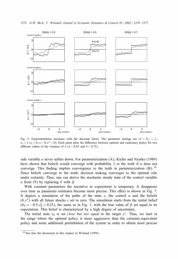
Fig. 4 serves to show that the optimal extent of experimentation increases with thedegree of persistence. The persistence parameter � is set to 0:5 (solid line) and 1 (dottedline), respectively. Fig. 5 similarly shows that the decision-maker is more willing toexperiment the more he cares about future rewards, that is, the greater the discountfactor. The comparison is for �= 0:75 and �= 0:95, respectively.

Of more fundamental interest may be the question whether the incentive to ex-periment is greater in an environment with constant or with time-varying unknownparameters. The answer to this question is provided in Fig. 6. The optimal extent ofexperimentation when � is a constant parameter (� = 0) is shown by the dotted line.


_3

0

3

Control Variable u

b =

_ 0.3

SD(b) = 0.3 SD(b) = 0.5

σε=1

σε=0.5

SD(b) = 0.7

_3

0

3

Control Variable u

b =

_ 0.5

_2 0 2

_3

0

3

Control Variable u

b =

_ 0.7

State Variable x



Fig. 3. Experimentation increases with the variance of shocks. The parameter settings are (� = 0; � = 1;� = 0; ! = 0; u∗ = 0; � = 0:95). Each panel plots the diEerence between optimal and cautionary policy fortwo diEerent values of the variance of � (� = 1 and � = 0:5).

The case of a time-varying, random-walk parameter, where any shock � has a perma-nent impact on the unknown parameter � is depicted by the solid line (� = 0:04).In spite of the diQculty in providing a very precise approximation to the extent ofexperimentation, it is clear from this comparison that the degree of experimentation issmaller when the parameter � is believed to change over time. The reason of course,is that the information gain resulting from experimentation is shorter-lived when theunknown parameter changes over time and follows a random walk. 9

4. Convergence

Having compared the optimal decision rule with learning to two alternative rulesof interest, we now turn to the question of convergence of beliefs and actions. Weconsider three diEerent parameterizations of the linear process de5ned by (1).

9 From this result, we conjecture that experimentation may be relatively more bene5cial if the unobservedparameter is assumed to exhibit mean revision, as in the example given in footnote 2. Although � alsochanges in this case, the information gain from experimentation may be more valuable since � remainsnearer to some average value. Whether this conjecture holds is a question for future study.


_3

0

3

Control Variable u

b =

_ 0.3

SD(b) = 0.3 SD(b) = 0.5

γ=1

γ=0.5

SD(b) = 0.7

_3

0

3

Control Variable u

b =

_ 0.5

_2 0 2

0

3

Control Variable u

b =

_ 0.7

State Variable x

0 2State Variable x

0 2State Variable x

_3

_2 _2

Fig. 4. Experimentation increases with the degree of persistence. The parameter settings are (� = 0; � = 1;� = 0; ! = 0; u∗ = 0; � = 0:95). Each panel plots the diEerence between optimal and cautionary policy fortwo diEerent values of the variance of � (� = 1 and � = 0:5).

(A) Simple regression with constant parameters (�= 0, � constant)

xt = �+ �ut + �t : (11)

In this scenario, the value chosen for u, if the parameters � and � were known, isconstant. Kiefer and Nyarko (1989) show that beliefs (b; vb) and actions u converge inthe limit. However, if u converges “too” quickly, then beliefs may converge to incorrectvalues and the limit action may be incorrect (at least when both, � and �, are unknown).For a further characterization of potential limit beliefs, see Kiefer and Nyarko (1989).Wieland (2000a, 2000b) computes optimal policies for such regressions and studiesthe likelihood of incomplete learning and the properties of time series generated underalternative policies.

(B) Regression with lagged dependent variable and constant parameters (� �=0,� constant)

xt = �+ �ut + �xt−1 + �t : (12)

In this case, the random shocks � have a persistent eEect on the dependent variable x.There is need for repeated stabilizing action by the decision-maker and the right-hand


0

3

Control Variable u

b =

_ 0.3

b =

_ 0.5

b =

_ 0.7

SD(b) = 0.3 SD(b) = 0.5

δ=0.95

δ=0.75

SD(b) = 0.7

0

3

Control Variable u

_2 _2 _20 2

_3

_3

_3

0

3

Control Variable u

State Variable x

0 2State Variable x

0 2State Variable x

Fig. 5. Experimentation increases with the discount factor. The parameter settings are (� = 0; � = 1;� =1; � =0; !=0; u∗ =0). Each panel plots the diEerence between optimal and cautionary policy for twodiEerent values of the variance of � (� = 0:95 and � = 0:75).

side variable u never settles down. For parameterization (A), Kiefer and Nyarko (1989)have shown that beliefs would converge with probability 1 to the truth if u does notconverge. This 5nding implies convergence to the truth in parameterization (B). 10

Since beliefs converge to the truth, decision making converges to the optimal ruleunder certainty. Thus, one can derive the stochastic steady state of the control variableu from (9) by replacing b with �.

With constant parameters the incentive to experiment is temporary. It disappearsover time as parameter estimates become more precise. This eEect is shown in Fig. 7.It depicts a simulation of the paths of the state x, the control u and the beliefs(b; vb) with all future shocks � set to zero. The simulation starts from the initial belief(b0 =−0:5; vb0 = 0:25), the same as in Fig. 1, with the true value of � set equal to itsexpectation. This belief is characterized by a high degree of uncertainty.

The initial state x0 is set close but not equal to the target x∗. Thus, we start inthe range where the optimal policy is more aggressive than the certainty-equivalentpolicy and some additional perturbation of the system in order to obtain more precise

10 See also the discussion in this respect in Wieland (1998).


_3

0

3

Control Variable u

b =

_0.

3

SD(b) = 0.3 SD(b) = 0.5

ση=0.0

ση=0.04

SD(b) = 0.7

0

3

Control Variable u

b =

_0.

5

_2 0 2

0

3

Control Variable u

b =

_0.

7

State Variable x

0 2State Variable x

0 2State Variable x

_3

_3

_2 _2

Fig. 6. Experimentation is lower with time-varying parameter. The parameter settings are (� = 0; � = 1;� = 1; ! = 0; u∗ = 0; � = 0:95). Each panel plots the diEerence between optimal and cautionary policy fortwo diEerent values of the variance of � (� = 0 and � = 0:04).

parameter estimates in the future is optimal. This can be seen from two top panelsof Fig. 7. The top left panel indicates that the small initial deviation from target ispositive (0.01) and consequently induces a positive response in the control variable(top right panel). The paths of x and u simulated in these two panels indicate thatthe optimal decision rule perturbs the system and induces >uctuations in x for about20 periods. It is important to understand that none of these >uctuations are caused byshocks, since current and future shocks have been set to zero. Rather, the >uctuationsin x are generated by the decision-maker in order to improve the precision of futureestimates of �.

The gain in the precision of the parameter estimates is directly apparent from thedecline in the variance, vb, shown in the lower right panel of Fig. 7. Once this vari-ance has fallen far enough, in this case to about 0.1 given a point estimate of −0:5,>uctuations in the control and state variables essentially cease, because the incentiveto experiment has disappeared.

The lower right panel of Fig. 7 reports the associated path of the point estimatebt , which remains constant throughout the whole period. This should not be surpris-ing, because the parameter estimate is only revised in response to forecast errors as


0 20 40 60 80 100

_0.1

_0.2

0

0.1

0.2

0.3

No. of Periods

xt

0 20 40 60 80 100 _1

_0.5

0

0.5

1

No. of Periods

ut

0 20 40 60 80 100 _1

_0.8

_0.6

_0.4

_0.2

0

No. of Periods

bt

0 20 40 60 80 1000

0.05

0.1

0.15

0.2

0.25

No. of Periods

vtb

Fig. 7. Dynamic simulation with constant parameters—no shocks. Initial beliefs are set to (b0 = −0:5;vb0 = 0:25). The initial state is x0 = 0:01. The parameter settings are (� = 0; � = 1; � = 1; � = 0;! = 0; u∗ = 0; � = 0:95). The shocks � are set to zero and � = b0.

discussed in Section 2. As long as no unexpected shocks occur, the forecasts of thedecision-maker are correct and the initial parameter estimate is con5rmed.

(C) Regression with lagged dependent variable and time-varying parameter(�¿ 0)

xt = �+ �tut + �xt−1 + �t : (13)

As in parameterization (B), actions u do not converge, because the shocks � continu-ously excite the system. Now however, a long-run limit for the beliefs (b; vb) does notexist. Since the decision-maker assumes that the unknown parameter follows a randomwalk, the variance of the parameter estimate increases every period by the variance ofthe shock to the unobserved parameter, that is �. As a result, uncertainty and conse-quently the incentive to experiment remain high, and the decision-maker continues toinduce some level of >uctuations. This eEect is illustrated in Fig. 8, which depicts asimulation starting from the same initial conditions as the simulation with a constantunobserved parameter in Fig. 7. Again, all current and future shocks (both � and �) areset to zero. As can be seen from the top two panels, the decision-maker again startsto induce >uctuations in order to improve the precision of the parameter estimate.


0 20 40 60 80 100-0.4

-0.3

-0.2

-0.1

0

0.1

0.2

0.3

No. of Periods

xt

0 20 40 60 80 100 -1.5

-1

-0.5

0

0.5

1

1.5

No. of Periods

ut

0 20 40 60 80 100 -1

-0.8

-0.6

-0.4

-0.2

0

No. of Periods

bt

0 20 40 60 80 1000

0.1

0.2

0.3

0.4

0.5

0.6

0.7

No. of Periods

vtb

Fig. 8. Dynamic simulation with time-varying parameter—no shocks. Initial beliefs are set to (b0 = −0:5;vb0 = 0:25). The initial state is x0 = 0:01. The parameter settings are (� = 0; � = 1; � = 1; � = 0:1;! = 0; u∗ = 0; � = 0:95). The shocks � and � are set to zero and � = b0.

However, because uncertainty regarding this parameter is renewed in every period(lower right panel), the incentive to experiment never ceases and the system exhibits asmall level of endogenous >uctuations even when all stochastic shocks are set to zero.

5. Conclusion

Using numerical approximations of optimal decision rules in a Bayesian learningproblem with unknown, potentially time-varying parameters and lagged dependent vari-ables, we found that the optimal behavior involves a noticeable degree of experimen-tation for moderate to large levels of parameter uncertainty. Nevertheless, the optimaldecision rule, in most cases, remains less aggressive than a certainty-equivalent rule.Thus, even the dynamically optimal decision rule with experimentation tends to inducegradualism. Exceptions occur when the linear process to be controlled is near the deter-ministic steady state. In this case, the incentive to experiment is strong enough to induceactivism, that is, a more aggressive action than under the certainty-equivalent rule. Ifthe unknown multiplicative parameter is perceived to vary over time, the incentive to


experiment is reduced. However, since parameter uncertainty in the time-varying pa-rameter case is renewed again and again, the incentive to experiment never disappearsas would be the case with constant parameters. Possible applications of the frameworkstudied in this paper arise, for example, in the areas of monopolistic pricing, investmentand growth and optimal policymaking under uncertainty.

References

Aghion, P., Bolton, P., Harris, C., Jullien, B., 1991. Optimal learning by experimentation. Review ofEconomic Studies 58, 621–654.

Amman, H., Kendrick, D., 1994a. Active learning: Monte Carlo results. Journal of Economic Dynamics andControl 18 (1), 119–124.

Amman, H., Kendrick, D., 1994b. Nonconvexities in stochastic control models: an analysis. In: Cooper,W.W., Whinston, A.B. (Eds.), New Directions in Computational Economics. Kluwer Academic Publishers,Dordrecht, pp. 57–94.

Amman, H., Kendrick, D., 1995. Nonconvexities in stochastic control models. International Economic Review36 (2), 455–475.

Anderson, T., Taylor, J.B., 1976. Some experimental results on the statistical properties of least squaresestimates in control problems. Econometrica 44, 1289–1302.

Balvers, R., Cosimano, T., 1994. In>ation variability and gradualist monetary policy. Review of EconomicStudies 61, 721–738.

Bar-Shalom, Y., Tse, E., 1976. Caution, probing and the value of information in the control of uncertainsystems. Annals of Economic and Social Measurement 4 (2), 239–252.

Easley, D., Kiefer, N.M., 1988. Controlling a stochastic process with unknown parameters. Econometrica 56,1045–1064.

Harvey, A., 1992. Time Series Models, 2nd Edition. MIT Press, Cambridge.Kendrick, D., 1978. Non-convexities from probing an adaptive control problem. Economic Letters 1,

347–351.Kendrick, D., 1979. Adaptive control of macroeconomic models with measurement error. In: Holly, S.,

Rustem, B., Zarrop, M.B. (Eds.), Optimal Control of Econometric Models. Macmillan, London,pp. 204–230.

Kendrick, D., 1981. Stochastic control for economic models. In: Economic Handbook Series. McGraw-Hill,New York.

Kendrick, D., 1982. Caution and probing in a macroeconomic model. Journal of Economic Dynamics andControl 4, 149–170.

Kiefer, N., 1989. A value function arising in the economics of information. Journal of Economic Dynamicsand Control 13, 201–223.

Kiefer, N., Nyarko, Y., 1989. Optimal control of an unknown linear process with learning. InternationalEconomic Review 30, 571–586.

Lai, T., Wei, C., 1982. Least squares estimates in stochastic regression models with applications toidenti5cation and control of dynamic systems. The Annals of Statistics 10 (1), 154–166.

MacRae, E., 1972. Linear decision with experimentation. Annals of Economic and Social Measurement 1,437–447.

Mizrach, B., 1991. Nonconvexities in a stochastic control problem with learning. Journal of EconomicDynamics and Control 15, 515–538.

Nyarko, Y., 1991. The number of equations versus the number of unknowns: the convergence of Bayesianposterior processes. Journal of Economic Dynamics and Control 15, 687–713.

Prescott, E., 1972. The multi-period control problem under uncertainty. Econometrica 40 (6), 1043–1058.Taylor, J.B., 1974. Asymptotic properties of multi-period control rules in the linear regression model.

International Economic Review 15, 472–484.Tse, E., Bar-Shalom, Y., 1973. An actively adaptive control for linear systems with random parameters.

IEEE Transactions on Automatic Control AC-18, 109–117.


Wieland, V., 1998. Monetary policy under uncertainty about the natural unemployment rate. Finance andEconomics Discussion Series, Board of Governors of the Federal Reserve System, pp. 98–122.

Wieland, V., 2000a. Learning by doing and the value of optimal experimentation. Journal of EconomicDynamics and Control 24, 501–534.

Wieland, V., 2000b. Monetary policy, parameter uncertainty and optimal learning. Journal of MonetaryEconomics 46, 199–228.

learning and control in a changing economic environment

Documents