learning by redundancy: how climate multi-model ensembles can help to fight the uncertainty

Learning by Redundancy: Climate Multi-Model Ensembles

and Machine Learning

Matteo De FeliceENEA, Climate Modeling Laboratory

Outline

• Why (what) Climate Ensembles?

• Dealing with uncertainty

• An example from the real world

Climate Models• Mathematical equations (physical processes) for each grid point

• Massive use of supercomputing

Climate Models• Mathematical equations (physical processes) for each grid point

• Massive use of supercomputing

“There are many more ways to be wrong in a 106

dimensional space than there are ways to be right.” Leonard Smith

Climate Models

from Alexander & Easterbrook, The software architecture of climate models: a graphicalcomparison of CMIP5 and EMICAR5 configurations, Geosci. Model Dev, 2015

Modelling the reality

Dealing with uncertainty"Doubt is not a pleasant condition, but certainty is absurd"

-Voltaire

Dealing with uncertainty

‣ How to deal with the uncertainty of parameters and/or initial conditions?

"Doubt is not a pleasant condition, but certainty is absurd" -Voltaire



‣ Climate Ensembles: running a model with (slightly) different conditions/parameters




‣ Climate Ensembles: running a model with (slightly) different conditions/parameters

‣ Approach used operationally since 1990s


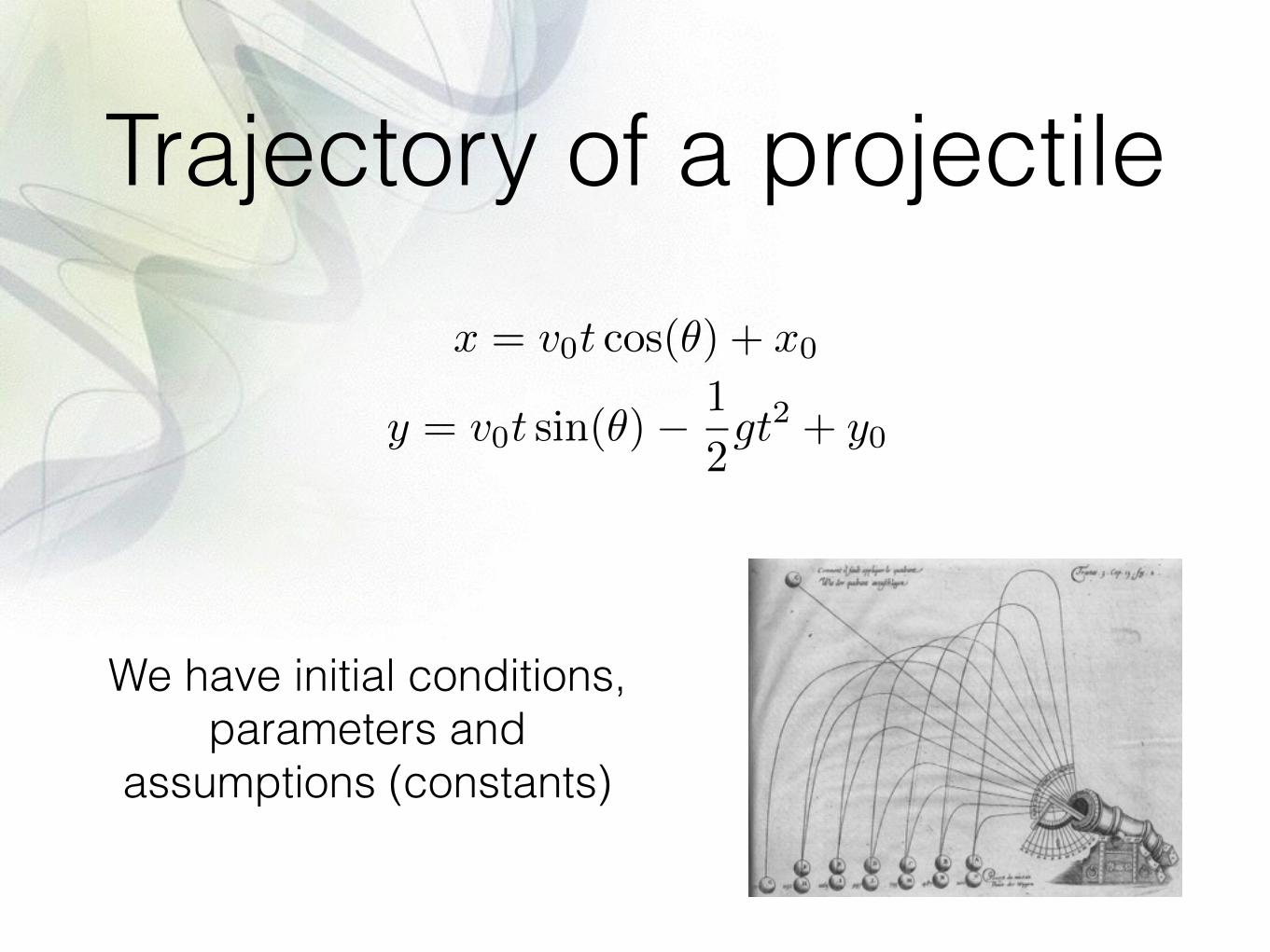
Trajectory of a projectile

y = v0t sin(✓)�1

2gt2 + y0

x = v0t cos(✓) + x0

We have initial conditions, parameters and

assumptions (constants)

What we (do not) know

What we (do not) knowWe can divide our knowledge in:


• “known knowns”: facts we know with certainty (e.g. gravitational acceleration on Earth)



• “known unknowns”: gaps we know exist (e.g. initial velocity or initial conditions)



• “known unknowns”: gaps we know exist (e.g. initial velocity or initial conditions)

• “unknown unknowns”: gaps we are unaware of (e.g. what if something like air resistance term?)

Ensemble Models“Initial velocity is 25 m/s and theta is 40°”

“Initial velocity is 25 m/s and theta is about 40°”

“Initial velocity is about 25 m/s and theta is about 40°”

“Initial velocity is about 25 m/s, theta is about 40° and x0 and y0 are between -1 and 1”

Back to reality

• Climate ensembles are needed, are used (and they are filling up our data storage)

Multi-models

Multi-models• Each ensemble member is a ‘what if’ scenario


• Combining structurally different climate (ensemble) models



• Example: IPCC AR4 is based on 23 climate models



• Example: IPCC AR4 is based on 23 climate models

Examples: EUROSIP (4 models),

NMME (7 models)

Redundancy (1)

Redundancy (1)

• The information contained into multi-model ensembles is redundant

Redundancy (1)

• The information contained into multi-model ensembles is redundant

• In Information Theory redundancy helps against the ‘noise’

Multi-models

Multi-models

• Multi-model ensembles are generally better…

Multi-models

• Multi-model ensembles are generally better…

• …than the average single-model performance

"Essentially, all models are wrong, but some are useful"

George E. P. Box

UncertaintyProbabilistic prediction of the 11+5 climate models of Summer precipitation above-normal over East-Asia

Data or information?

Data Information“factual information (as

measurements or statistics) used as a basis for reasoning,

discussion, or calculation” ( Merriam-Webster)

“knowledge obtained from investigation, study, or

instruction”( Merriam-Webster)

?

Data or information?

Data Information“factual information (as

measurements or statistics) used as a basis for reasoning,

discussion, or calculation” ( Merriam-Webster)

“knowledge obtained from investigation, study, or

instruction”( Merriam-Webster)

?

DRIP (Data Rich Information Poor) era

Information hiding double time(time) ; time:standard_name = "time" ; time:long_name = "Time in days" ; time:units = "days since 1950-01-01 00:00:00" ; time:calendar = "standard" ; short pp(time, latitude, longitude) ; pp:standard_name = "air_pressure_at_sea_level" ; pp:long_name = "sea level pressure" ; pp:units = "hPa" ; pp:add_offset = 0.f ; pp:scale_factor = 0.1f ; pp:_FillValue = -9999s ; pp:missing_value = -9999s ;

// global attributes: :CDI = "Climate Data Interface version 1.6.4 (http://code.zmaw.de/projects/cdi)" ; :Conventions = "CF-1.4" ; :history = "Tue Jan 13 15:48:45 2015: cdo sellonlatbox,-45,60,30,68 pp_0.50deg_reg_v10.0.mon.nc pp_0.50deg_reg_v10.0.mon.EUROPE.nc\n", "Tue Jan 13 15:46:58 2015: cdo -monavg pp_0.50deg_reg_v10.0.nc pp_0.50deg_reg_v10.0.mon.nc" ; :Ensembles_ECAD = "10.0" ; :References = "http://www.ecad.eu\\nhttp://www.ecad.eu/download/ensembles/ensembles.php\\nvan den Besselaar et al. (2011) J. Geophys. Res., 116, D11110, http://dx.doi.org/10.1029/2010JD015468" ; :CDO = "Climate Data Operators version 1.6.4 (http://code.zmaw.de/projects/cdo)" ;data:

longitude = -40.25, -39.75, -39.25, -38.75, -38.25, -37.75, -37.25, -36.75, -36.25, -35.75, -35.25, -34.75, -34.25, -33.75, -33.25, -32.75, -32.25, -31.75, -31.25, -30.75, -30.25, -29.75, -29.25, -28.75, -28.25, -27.75, -27.25, -26.75, -26.25, -25.75, -25.25, -24.75, -24.25, -23.75, -23.25, -22.75, -22.25, -21.75, -21.25, -20.75, -20.25, -19.75, -19.25, -18.75, -18.25, -17.75, -17.25, -16.75, -16.25, -15.75, -15.25, -14.75, -14.25, -13.75, -13.25, -12.75, -12.25, -11.75, -11.25, -10.75, -10.25, -9.75, -9.25, -8.75, -8.25, -7.75, -7.25, -6.75, -6.25, -5.75, -5.25, -4.75, -4.25, -3.75, -3.25, -2.75, -2.25, -1.75, -1.25, -0.75, -0.25, 0.25, 0.75, 1.25, 1.75, 2.25, 2.75, 3.25, 3.75, 4.25, 4.75, 5.25, 5.75, 6.25,

How to evaluate data and information

It is often said that we suffer from “information overload,” whereas we actually suffer from “data overload.” The problem is that we have access to large amounts of data containing relatively

small amounts of useful information.INDEPENDENT COMPONENT ANALYSIS A Tutorial

Introduction James V. Stone

Dealing with this

Improve the knowledge about physical processes

Extract the maximum amount of information from climate data

improve process-realism, better resolution, more advanced schemes

…TBD…

Dealing with this

Improve the knowledge about physical processes

Extract the maximum amount of information from climate data

improve process-realism, better resolution, more advanced schemes

…TBD…

The sad truth of climate science is that the most crucial

information is the least reliable. (Q. Schiermeier, Nature,

2010)

Existing research

• Climate Informatics

• Data-Driven Knowledge Discovery in Climate Science (V. Kumar Uni of Minnesota)

“climate informatics could be defined as data-driven inquiry, and hence offers a complement to existing approaches to climate science.”

Data-driven discovery• Creation of a climate

network (see works by J. Donges and A. Tsonis)

• Two purposes: understanding climate dynamics and evaluate climate models

• Results: already known dipoles discovered and new dipoles (unknown phenomena?)

• What about the casual relationship?

from Kawale et al., SDM, 2015

A (personal) to-do list


1) “Better” metrics (more context-related)



2) Better dimensionality reduction methods



2) Better dimensionality reduction methods

3) (more) use of advanced & non-linear classification/regression methods

Example in energy• Impacts: no standard approaches

• ENEA experience with TERNA (question-driven research)

• Main themes: electricity demand, solar power, electricity exchange

Electricity demandCan we predict electricity demand using weather information?

Past demand

Obs. weathermodel

Weather forecasts

Future demand

What about the next months?

• From weather forecasts to climate forecasts

(a) System4 - April (b) System4 - May

Figure 2: Correlation coe�cient between June-July temperature anomaly de-rived by ERA-INTERIM dataset on years 1990-2007 and System4 forecast. Dotsrepresents points with a 5% of significance calculated by bootstrapping.

(a) System4 - 1st Pattern (b) System4 - 2nd Pattern (c) System4 - 3rd Pattern

(d) System4 - 1st PC (e) System4 - 2nd PC (f) System4 - 3rd PC

(g) ERA-IN - 1st Pattern (h) ERA-IN - 2nd Pattern (i) ERA-IN - 3rd Pattern

(j) ERA-IN - 1st PC (k) ERA-IN - 2nd PC (l) ERA-IN - 3rd PC

Figure 3: First three patterns with relative coe�cients obtained using PrincipalComponent Analysis on System4 and ERA-INTERIM temperature data. Thethree patterns represent for System4 and ERA-INTERIM respectively the 37.4%and 49.4% of total variance

5

Two big shifts1) From deterministic to probabilistic forecasting

> Target: 30.1 GW> Forecast: 30.4 GW

> Target: 30.1 GW> Forecast mean: 29.82 GW > Forecast sd: 5.04 GW

> Target: demand more than normal> Forecast: 74% of having demand above normal

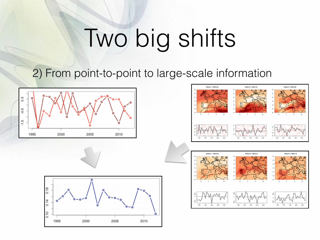
Two big shifts2) From point-to-point to large-scale information

Electricity demand for the next months


1.Predictand has become “electricity demand above/below normal”


1.Predictand has become “electricity demand above/below normal”

2.Predictors are the main patterns of the entire ensemble

Temperature forecast

member 1 1990-2007


member 2 1990-2007


member 51 1990-2007

time [n.years x n.members]

spac

e [la

t x lo

n po

ints

]

…

Prediction approachTemp. PC 1

Temp. PC 2

Temp. PC 3

Temp. PC n

…

SVM

Optional: other variables

Electricity demand

Non-linear regression/classification method

Final product

De Felice M., Alessandri A., and F. Catalano, “Seasonal climate forecasts for medium-term electricity demand forecasting,” Applied

Energy, vol. 137, pp. 435-444, 2015

Electricity Exchange

European electricity flows for Jan-Feb (left) and June-July (right) – red nodes are the main exporters and blue the main importers – Data from ENTSO-E

(2003-2014)

Data flows

Weather/Climate

observations & forecasts

+

Random Forest / Naive Bayes

Extracting information• Is France electricity export driven by temperature? • Use of climate forecasts and lagged indices to predict “high export” events (Jan-Feb)

Random Forest

1000 decision trees computed in LOO-CV Brier Skill Score: 0.17 Variable importance:

1. NAO (OND)2. Temperature PC4 (9% var) 3. Temperature PC5 (6% var)

Naive Bayes Computed in LOO-CV Brier Skill Score: 0.36

Redundancy (2)

Redundancy (2)• Redundancy not in the ‘inputs’ but in the models


• Combining multiple classifiers/regressors improve the performance


• Combining multiple classifiers/regressors improve the performance

• Good ensembles when individual components make their errors in different parts of the input space

Concluding remarks

The uncertainty monster

Curry & Webster, Climate Science and the Uncertainty Monster, BAMS, 2011

The uncertainty monster• Monster hiding: never admit the error!



• Monster exorcism




• Monster simplification: quantification and simplification of the uncertainty assessment





• Monster detection: extending science’s frontiers





• Monster detection: extending science’s frontiers

• Monster assimilation:learning to live with the monster
