learning curve in modern ml the 'double descent' behavior
TRANSCRIPT

Learning curve in modern MLThe ”double descent” behavior
Oren Yuval
Department of Statistics and Operations Research
Tel-Aviv University
December 23, 2019
Oren Yuval Learning curve in modern ML , The ”double descent” behavior 1 / 47

Outline
1 Background
2 Main findings
3 Real data simulations
4 Theoretical analysis for Least-Squares
5 Summery
Oren Yuval Learning curve in modern ML , The ”double descent” behavior 2 / 47

Background
The classical learning curve
We all know the Bias-Variance Trade-Off:
The common knowledge - very low training error → very high variance
One may think of some criteria for finding the optimal model
Oren Yuval Learning curve in modern ML , The ”double descent” behavior 3 / 47

Background
The classical learning curve
We all know the Bias-Variance Trade-Off:
The common knowledge - very low training error → very high variance
One may think of some criteria for finding the optimal model
Oren Yuval Learning curve in modern ML , The ”double descent” behavior 3 / 47

Background
The classical learning curve
We all know the Bias-Variance Trade-Off:
The common knowledge - very low training error → very high variance
One may think of some criteria for finding the optimal model
Oren Yuval Learning curve in modern ML , The ”double descent” behavior 3 / 47

Background
Is NN immune to variance?
On the other hand - very rich models such as NN are trained to exactly fitthe train data, and yet they obtain high accuracy on test data
How can we reconcile the modern practice with the classical bias-variancetrade-off?
Oren Yuval Learning curve in modern ML , The ”double descent” behavior 4 / 47

Background
A ”jamming transition”
Spigler in mid 2018, argued that in fully-connected networks, a phasetransition delimits the over and under-parametrized regimes where fittingcan or cannot be achieved
Oren Yuval Learning curve in modern ML , The ”double descent” behavior 5 / 47

Background
Reconciling the discrepancy
Just one year ago - Belkin et al first analyzed the behavior of rich modelsaround the interpolation point
Since then many authors published results, that justified the innovativeapproachHastie, Rosset, and Tibshirani provided a precise quantitative explanationfor the potential benefits of over-parametrization in linear regression
Oren Yuval Learning curve in modern ML , The ”double descent” behavior 6 / 47
Background
Reconciling the discrepancy
Just one year ago - Belkin et al first analyzed the behavior of rich modelsaround the interpolation point
Since then many authors published results, that justified the innovativeapproach
Hastie, Rosset, and Tibshirani provided a precise quantitative explanationfor the potential benefits of over-parametrization in linear regression
Oren Yuval Learning curve in modern ML , The ”double descent” behavior 6 / 47

Background
Reconciling the discrepancy
Just one year ago - Belkin et al first analyzed the behavior of rich modelsaround the interpolation point
Since then many authors published results, that justified the innovativeapproachHastie, Rosset, and Tibshirani provided a precise quantitative explanationfor the potential benefits of over-parametrization in linear regression
Oren Yuval Learning curve in modern ML , The ”double descent” behavior 6 / 47

Background
Empirical risk minimization
Given a training sample (x1, y1), · · · , (xn, yn), where (xi , yi ) ∈ Rd × R,
we learn a predictor hn : Rd → R.
In ERM, the predictor is taken to be
hn = argminh∈H
{1
n
n∑i=1
l (yi , h(xi ))
}
Empirical risk (train error): 1n
∑ni=1 l (yi , hn(xi ))
Interpolation: l (yi , hn(xi )) = 0 ∀i
True risk (test error): Ex ,y [l (yi , hn(xi ))]
Oren Yuval Learning curve in modern ML , The ”double descent” behavior 7 / 47

Background
Controlling H
Conventional wisdom in machine learning suggests controlling the capacityof H:
H too small → under-fitting (large empirical and true risk)
H too large → over-fitting (small empirical risk but large true risk)
Example (OLS)
β̂n = argminβ∈Rp
{1
n
n∑i=1
(yi − xTi β
)2}
True risk ∝ pn−p
Yet, best practice in DL: network should be large enough to permiteffortless zero train-loss
Oren Yuval Learning curve in modern ML , The ”double descent” behavior 8 / 47

Main findings
The “double descent” risk curve
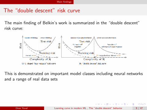
The main finding of Belkin’s work is summarized in the “double descent”risk curve:
This is demonstrated on important model classes including neural networksand a range of real data sets
The capacity of H is identified with the number of parameters needed tospecify the function hn
Oren Yuval Learning curve in modern ML , The ”double descent” behavior 9 / 47
Main findings
The “double descent” risk curve
The main finding of Belkin’s work is summarized in the “double descent”risk curve:
This is demonstrated on important model classes including neural networksand a range of real data sets
The capacity of H is identified with the number of parameters needed tospecify the function hn
Oren Yuval Learning curve in modern ML , The ”double descent” behavior 9 / 47

Main findings
Fitting beyond the interpolation point
When zero train error can be achieved, we choose hn as follows:
hn = argminh∈H
{||hn|| s.t :
1
n
n∑i=1
l (yi , h(xi )) = 0
}
Looking for the simplest/smoothest function that explain the data
By increasing the capacity of H, we are able to find interpolatingfunctions that have smaller norm
Oren Yuval Learning curve in modern ML , The ”double descent” behavior 10 / 47

Main findings
Why is the “double descent” important?
Stating that interpolation does not necessarily lead to poorgeneralization, as long as you ”deep” enough in the interpolationregime
Reconciling the modern practice with a statistical point-of-view
Explicit analysis for Linear Models
The true risk in the over-parameterized regime is typically lower!
Oren Yuval Learning curve in modern ML , The ”double descent” behavior 11 / 47

Real data simulations
Neural networks
One Hidden layer with N random features
Minimizing squared loss or ||a||2 when N ≥ n
x̃k = ϕ(x ; vk) = ϕ(< x , vk >) , vk ∼ MN(0, Ip)
Oren Yuval Learning curve in modern ML , The ”double descent” behavior 12 / 47

Real data simulations
Neural networks
Risk curve for RFF model onMNIST
Near interpolation -parameters are ”forced”to fit the training data
Increasing N results indecreasing the l2 norm ofthe predictors
Oren Yuval Learning curve in modern ML , The ”double descent” behavior 13 / 47

Real data simulations
Neural networks
Fully connected two-layers network with H hidden units
Optimizing the weight using SGD with up to 6 · 103 iterations:
Interpolation is not assured even in the over-parameterized regime
Automatically prefers minimal-norm solution
Sub-optimal behavior canlead to high variability inboth the training and testrisks that masks the doubledescent curve
Oren Yuval Learning curve in modern ML , The ”double descent” behavior 14 / 47

Real data simulations
Neural networks
Risk curves for two-Layersfully connected NN onMNIST
Train risk may increasewith increasing numberof parameters
Oren Yuval Learning curve in modern ML , The ”double descent” behavior 15 / 47

Real data simulations
Decision trees
It was shown by Wyner et al (2017) that AdaBoost and Random-Forestsperform better with large (interpolating) decision trees and are morerobust to noise in the training data
They questioned the conventional wisdom that suggests that boostingalgorithms for classification requires regularization/early stopping/lowcomplexity
The effect of noise-pointon a classifier:interpolating Vsnon-interpolating
Oren Yuval Learning curve in modern ML , The ”double descent” behavior 16 / 47

Real data simulations
Decision trees
Risk curves forRandom-Forests on MNIST
The complexity iscontrolled by the size ofa decision tree, and thenumber of trees
Averaging ofinterpolating treesensures substantiallysmoother function
Oren Yuval Learning curve in modern ML , The ”double descent” behavior 17 / 47
Real data simulations
Thinking about it...
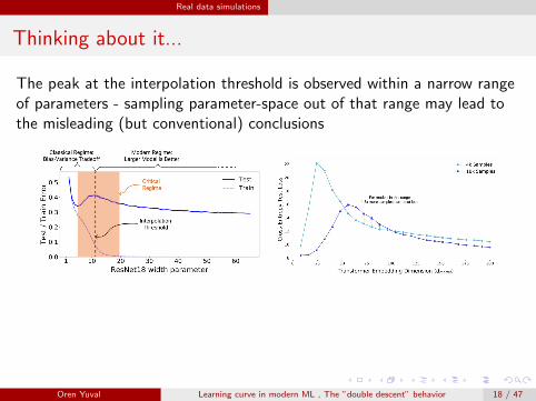
The peak at the interpolation threshold is observed within a narrow rangeof parameters - sampling parameter-space out of that range may lead tothe misleading (but conventional) conclusions
The understanding of the ”double descent” behavior is important forpractitioners to choose between models for optimal performance
Oren Yuval Learning curve in modern ML , The ”double descent” behavior 18 / 47

Real data simulations
Thinking about it...
The peak at the interpolation threshold is observed within a narrow rangeof parameters - sampling parameter-space out of that range may lead tothe misleading (but conventional) conclusions
The understanding of the ”double descent” behavior is important forpractitioners to choose between models for optimal performance
Oren Yuval Learning curve in modern ML , The ”double descent” behavior 18 / 47

Theoretical analysis for Least-Squares
Why Least-Squares?
Easy to analyze
Easy to explain
Easy to simulate
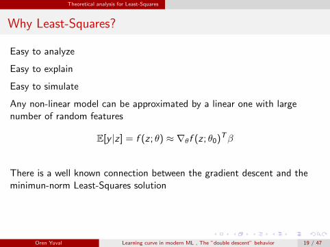
Any non-linear model can be approximated by a linear one with largenumber of random features
E[y |z ] = f (z ; θ) ≈ ∇θf (z ; θ0)Tβ
There is a well known connection between the gradient descent and theminimun-norm Least-Squares solution
Oren Yuval Learning curve in modern ML , The ”double descent” behavior 19 / 47

Theoretical analysis for Least-Squares
Why Least-Squares?
Easy to analyze
Easy to explain
Easy to simulate
Any non-linear model can be approximated by a linear one with largenumber of random features
E[y |z ] = f (z ; θ) ≈ ∇θf (z ; θ0)Tβ
There is a well known connection between the gradient descent and theminimun-norm Least-Squares solution
Oren Yuval Learning curve in modern ML , The ”double descent” behavior 19 / 47
Theoretical analysis for Least-Squares
The Linear model
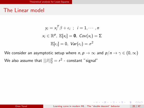
yi = xTi β + εi ; i = 1, · · · , n
xi ∈ Rp, E[xi ] = 0, Cov(xi ) = Σ
E[εi ] = 0, Var(εi ) = σ2
We consider an asymptotic setup where n, p →∞ and p/n→ γ ∈ (0,∞)
We also assume that ||β||22 = r2 - constant ”signal”
Some assumptions over the distribution of x may be taken:
x ∼ MN(0,Σ)
x = Σ1/2z , zj ∼ (0, 1)
Isotropic features: Σ = Ip
x = ϕ(Wz), where W ∈ Rp×d a random matrix with i.i.d. entries
Oren Yuval Learning curve in modern ML , The ”double descent” behavior 20 / 47

Theoretical analysis for Least-Squares
The Linear model
Assuming that the model is well-specified, the out-of-sample predictionrisk is:
R(β̂;β) = EXYx0
(xT0 β̂ − xT0 β
)2
Assuming isotropic features, we can decompose the risk to bias andvariance terms:
R(β̂;β) = EX
[||E[β̂|X ]− β||22
]+ EX
[tr [Cov(β̂|X )]
]:= B(β̂;β) + V (β̂)
Taking β̂ = (XTX )−1XTY , we get:
E[β̂|X ] = β ; Cov(β̂|X ) = σ2(XTX )−1 → σ2
n − pIp
and therefore R(β̂;β)→ σ2γ1−γ
Oren Yuval Learning curve in modern ML , The ”double descent” behavior 21 / 47

Theoretical analysis for Least-Squares
High dimensional Least-Squares
When γ > 1, the empirical risk ||Y − Xβ||22 can be eliminated, and we arelooking for the minimum l2 norm estimator :
β̂ = argminβ∈Rp
{||β||2 s.t : ||Y − Xβ||22 = 0
}
Solving with Lagrange multipliers:
argminβ,λ
{βTβ + λT (Y − Xβ)
}We get:
β̂ = XT λ̂ ; λ̂ = (XXT )−1Y =⇒ β̂ = XT (XXT )−1Y
One can write: β̂ = (XTX )+XTY
Oren Yuval Learning curve in modern ML , The ”double descent” behavior 22 / 47

Theoretical analysis for Least-Squares
High dimensional Least-Squares
When γ > 1, the empirical risk ||Y − Xβ||22 can be eliminated, and we arelooking for the minimum l2 norm estimator :
β̂ = argminβ∈Rp
{||β||2 s.t : ||Y − Xβ||22 = 0
}Solving with Lagrange multipliers:
argminβ,λ
{βTβ + λT (Y − Xβ)
}We get:
β̂ = XT λ̂ ; λ̂ = (XXT )−1Y =⇒ β̂ = XT (XXT )−1Y
One can write: β̂ = (XTX )+XTY
Oren Yuval Learning curve in modern ML , The ”double descent” behavior 22 / 47

Theoretical analysis for Least-Squares
Computing the bias term
Now we have:E[β̂|X ] = XT (XXT )−1Xβ 6= β
and therefore the bias term is:
B(β̂;β) = EX
[||E[β̂|X ]− β||22
]= βT (Ip − EX [XT (XXT )−1X ])β
We can show that EX [XT (XXT )−1X ]→ np Ip, and therefore:
B(β̂;β) = βTβ − n
pβTβ = r2(1− 1
γ)
Note that:
EX
[||E[β̂|X ]||22
]→ n
pr2 =
r2
γ
Oren Yuval Learning curve in modern ML , The ”double descent” behavior 23 / 47

Theoretical analysis for Least-Squares
Computing the variance term
Recall that:V (β̂) = EX
[tr [Cov(β̂|X )]
]Now we have:
Cov(β̂|X ) = σ2(XXT )−1XXT (XXT )−1 = σ2(XXT )−1 → σ2
p − nIn
and therefore:
V (β̂)→ σ2
γ − 1
Oren Yuval Learning curve in modern ML , The ”double descent” behavior 24 / 47

Theoretical analysis for Least-Squares
Limiting Risk
For the asymptotic setting, we can obtain the following formula:
A new bias-variance trade-off in the over-parameterized regime
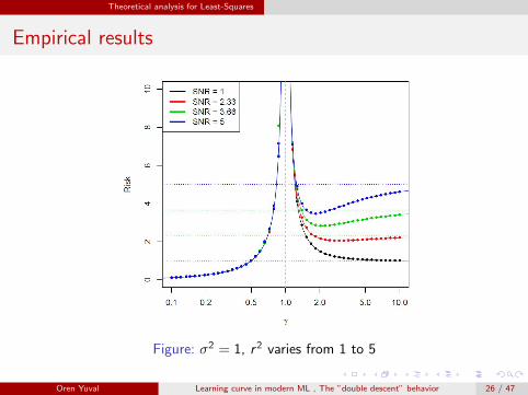
The behavior can be controlled by the SNR = r2/σ2
If SNR > 1, there is a local min at γ =√SNR√
SNR−1
As γ →∞, the estimator β̂ converge to the null estimator β̃ = 0, andthe total risk is r2
Oren Yuval Learning curve in modern ML , The ”double descent” behavior 25 / 47
Theoretical analysis for Least-Squares
Empirical results
Figure: σ2 = 1, r2 varies from 1 to 5
Oren Yuval Learning curve in modern ML , The ”double descent” behavior 26 / 47

Theoretical analysis for Least-Squares
Misspecified model
yi = xTi β + ωTi θ + εi ; i = 1, · · · , n
xi ∈ Rp, ωi ∈ Rd , E[(xi , ωi )] = 0, E[εi ] = 0, Var(εi ) = σ2
For simplicity, we assume that Cov((xi , ωi )) = Ip+d
In this case we can write:
yi = xTi β + δi ; i = 1, · · · , n
E[δi ] = 0, Var(δi ) = σ2 + ||θ||22
We also assume that ||β||22 + ||θ||22 = r2 - constant ”signal”
Oren Yuval Learning curve in modern ML , The ”double descent” behavior 27 / 47

Theoretical analysis for Least-Squares
Misspecified model
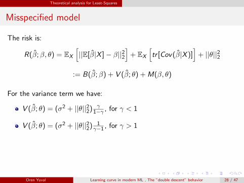
The risk is:
R(β̂;β, θ) = EX
[||E[β̂|X ]− β||22
]+ EX
[tr [Cov(β̂|X )]
]+ ||θ||22
:= B(β̂;β) + V (β̂; θ) + M(β, θ)
For the variance term we have:
V (β̂; θ) = (σ2 + ||θ||22) γ1−γ , for γ < 1
V (β̂; θ) = (σ2 + ||θ||22) 1γ−1 , for γ > 1
Oren Yuval Learning curve in modern ML , The ”double descent” behavior 28 / 47
Theoretical analysis for Least-Squares
Misspecified model
The risk is:
R(β̂;β, θ) = EX
[||E[β̂|X ]− β||22
]+ EX
[tr [Cov(β̂|X )]
]+ ||θ||22
:= B(β̂;β) + V (β̂; θ) + M(β, θ)
For the variance term we have:
V (β̂; θ) = (σ2 + ||θ||22) γ1−γ , for γ < 1
V (β̂; θ) = (σ2 + ||θ||22) 1γ−1 , for γ > 1
Oren Yuval Learning curve in modern ML , The ”double descent” behavior 28 / 47

Theoretical analysis for Least-Squares
Misspecified model
The total risk for γ < 1:
||θ||22 + (σ2 + ||θ||22)γ
1− γ
The total risk for γ > 1:
||θ||22 + ||β||22(1− 1
γ) + (σ2 + ||θ||22)
1
γ − 1
What can be a conventional connection between γ and ||θ||22?
How the signal is distributed over γ?
Oren Yuval Learning curve in modern ML , The ”double descent” behavior 29 / 47
Theoretical analysis for Least-Squares
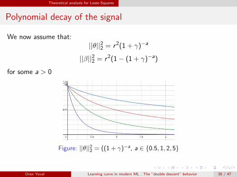
Polynomial decay of the signal
We now assume that:||θ||22 = r2(1 + γ)−a
||β||22 = r2(1− (1 + γ)−a)
for some a > 0
Figure: ||θ||22 = ((1 + γ)−a, a ∈ {0.5, 1, 2, 5}
Oren Yuval Learning curve in modern ML , The ”double descent” behavior 30 / 47
Theoretical analysis for Least-Squares
Polynomial decay of the signal
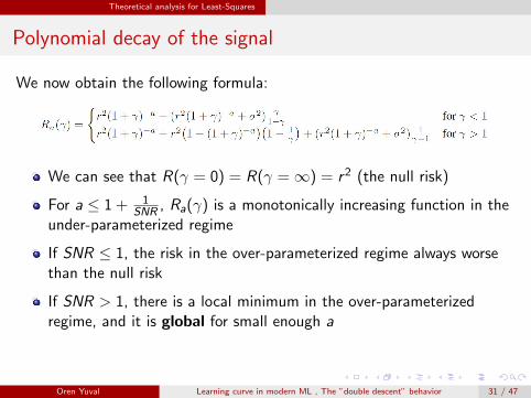
We now obtain the following formula:
We can see that R(γ = 0) = R(γ =∞) = r2 (the null risk)
For a ≤ 1 + 1SNR , Ra(γ) is a monotonically increasing function in the
under-parameterized regime
If SNR ≤ 1, the risk in the over-parameterized regime always worsethan the null risk
If SNR > 1, there is a local minimum in the over-parameterizedregime, and it is global for small enough a
Oren Yuval Learning curve in modern ML , The ”double descent” behavior 31 / 47

Theoretical analysis for Least-Squares
Empirical results
The ”double descent” behavior achieved...
Oren Yuval Learning curve in modern ML , The ”double descent” behavior 32 / 47
Theoretical analysis for Least-Squares
Thinking about it...
Yet, we did not see the same behavior as in the NN simulations...
The reason may be - the distribution of the signal over the parametersspace
What if - the majority of the signal is located within some range in theover-parameterized regime?
Figure: ||θ||22 = g(γ)
Oren Yuval Learning curve in modern ML , The ”double descent” behavior 33 / 47

Theoretical analysis for Least-Squares
Model evaluation
For the task of models evaluation and selection we may use theleave-one-out cross-validation estimator (CV for short):
CVn =1
n
n∑i=1
(yi − f̂ −in (xi )
)2
We may also want use the ”shortcut formula”:
CVn =1
n
n∑i=1
(yi − f̂n(xi )
1− Sii
)2
=1
n
n∑i=1
(yi − [SY ]i
1− Sii
)2
where S is the linear smoother matrix
Oren Yuval Learning curve in modern ML , The ”double descent” behavior 34 / 47

Theoretical analysis for Least-Squares
Model evaluation
For any linear interpolator:
SY = Y =⇒ S = In =⇒ yi − [SY ]i1− Sii
=0
0
in particular for the min-norm interpolator: S = XXT (XXT )−1 = In
Fortunately, we can solve this problem! Rewrite S to be:
S = XXT (XXT + λIn)−1 , λ→ 0+
Oren Yuval Learning curve in modern ML , The ”double descent” behavior 35 / 47

Theoretical analysis for Least-Squares
Model evaluation
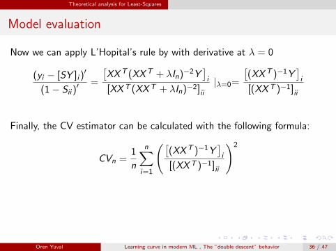
Now we can apply L’Hopital’s rule by with derivative at λ = 0
(yi − [SY ]i )′
(1− Sii )′ =
[XXT (XXT + λIn)−2Y
]i
[XXT (XXT + λIn)−2]ii|λ=0=
[(XXT )−1Y
]i
[(XXT )−1]ii
Finally, the CV estimator can be calculated with the following formula:
CVn =1
n
n∑i=1
([(XXT )−1Y
]i
[(XXT )−1]ii
)2
Oren Yuval Learning curve in modern ML , The ”double descent” behavior 36 / 47
Theoretical analysis for Least-Squares
Model evaluation
Now we can apply L’Hopital’s rule by with derivative at λ = 0
(yi − [SY ]i )′
(1− Sii )′ =
[XXT (XXT + λIn)−2Y
]i
[XXT (XXT + λIn)−2]ii|λ=0=
[(XXT )−1Y
]i
[(XXT )−1]ii
Finally, the CV estimator can be calculated with the following formula:
CVn =1
n
n∑i=1
([(XXT )−1Y
]i
[(XXT )−1]ii
)2
Oren Yuval Learning curve in modern ML , The ”double descent” behavior 36 / 47

Theoretical analysis for Least-Squares
Ridge regression
The min-norm estimator is related to the Ridge regression estimator asfollows:
β̂ = limλ→0+ β̂λ
where β̂λ is the Ridge regression estimator:
β̂λ = argminβ∈Rp
{1
n||Y − Xβ||22 + λ||β||2
}= (XTX + nλIp)−1XTY
Thus, an optimal tune β̂λ should be better than β̂
The limiting risk for the optimal β̂λ can be written explicitly as:
Oren Yuval Learning curve in modern ML , The ”double descent” behavior 37 / 47

Theoretical analysis for Least-Squares
Ridge regression
In overview looking we can simplify the optimal risk into:
R(β̂λ∗ ;β, θ) ≈ ||θ||22 + f (σ2; γ) + g(||β||22; γ)
where f (z ; γ)→ 0, g(z ; γ)→ z as γ →∞
and g(z ; 0) = f (z ; 0) = 0
Looks like trade-off between observed and unobserved signals
Again, the distribution of the signal over γ may play a role...
Oren Yuval Learning curve in modern ML , The ”double descent” behavior 38 / 47

Theoretical analysis for Least-Squares
Ridge regression - optimal risk curves
Oren Yuval Learning curve in modern ML , The ”double descent” behavior 39 / 47

Theoretical analysis for Least-Squares
Optimal risk curves - misspecified model
R(β̂λ∗ ;β, θ) ≈ ||θ||22 + f (σ2; γ) + g(||β||22; γ)
Optimal risk curves with||θ||22 = (1 + γ)−a, a = 2
Why is the minimum riskaround γ = 1?
”... it seems we want thecomplexity of the featurespace to put us as close tothe interpolation boundary aspossible...”
Oren Yuval Learning curve in modern ML , The ”double descent” behavior 40 / 47
Theoretical analysis for Least-Squares
Optimal risk curves - misspecified model
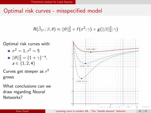
R(β̂λ∗ ;β, θ) ≈ ||θ||22 + f (σ2; γ) + g(||β||22; γ)
Optimal risk curves with:
σ2 = 1, r2 = 5
||θ||22 = (1 + γ)−a,a ∈ {1, 2, 4}
Curves get steeper as r2
grows
What conclusions can wedraw regarding NeuralNetworks?
Oren Yuval Learning curve in modern ML , The ”double descent” behavior 41 / 47

Theoretical analysis for Least-Squares
Additional results - nonlinear features
Asymptotic variance in a nonlinear feature model, x = ϕ(Wz)
Oren Yuval Learning curve in modern ML , The ”double descent” behavior 42 / 47
Theoretical analysis for Least-Squares
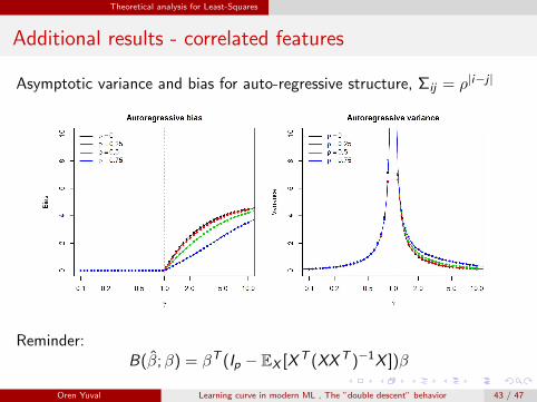
Additional results - correlated features
Asymptotic variance and bias for auto-regressive structure, Σij = ρ|i−j |
Reminder:B(β̂;β) = βT (Ip − EX [XT (XXT )−1X ])β
Oren Yuval Learning curve in modern ML , The ”double descent” behavior 43 / 47

Theoretical analysis for Least-Squares
Additional results - correlated features
Asymptotic risk for auto-regressive structure, Σij = ρ|i−j |
Oren Yuval Learning curve in modern ML , The ”double descent” behavior 44 / 47

Theoretical analysis for Least-Squares
CV-tuned Ridge regression
Finite-sample risks for CV-tuned ridge regression estimator compered toAsymptotic risk (20 independent training samples)
Oren Yuval Learning curve in modern ML , The ”double descent” behavior 45 / 47

Summery
Summary
There is a growing interest in Interpolators in ML
The double descent phenomenon must be well understood and taken intoaccount for model optimization
The linear model analysis explains the bias-variance trade-off in theinterpolation regime
The real-life trade-off:
Balance between signalobs -bias-variance
Controlled by complexity-regularization/early stopping
Oren Yuval Learning curve in modern ML , The ”double descent” behavior 46 / 47
