Learning Data Structure from Classes: A Case Study

Applied to Population Genetics

J. J. del Coza,∗, J. Dıeza, A. Bahamondea, F. Goyacheb

aArtificial Intelligence Center. University of Oviedo at Gijon, 33271 Asturias, Spainhttp://www.aic.uniovi.es

bSERIDA-Deva, Camino de Rioseco, Gijon, Asturias, Spain

Abstract

In most cases, the main goal of machine learning and data mining applications

is to obtain good classifiers. However, final users, for instance researchers in

other fields, sometimes prefer to infer new knowledge about their domain that

may be useful to confirm or reject their hypotheses. This paper presents a

learning method that works along these lines, in addition to reporting three

interesting applications in the field of population genetics in which the aim is

to discover relationships between species or breeds according to their geno-

types. The proposed method has two steps: first it builds a hierarchical

clustering of the set of classes and then a hierarchical classifier is learned.

Both models can be analyzed by experts to extract useful information about

their domain. In addition, we propose a new method for learning the hier-

archical classifier. By means of a voting scheme employing pairwise binary

models constrained by the hierarchical structure, the proposed classifier is

computationally more efficient than previous approaches while improving on

∗Corresponding authorEmail addresses: juanjo@aic.uniovi.es (J. J. del Coz), jdiez@aic.uniovi.es (J.

Dıez), antonio@aic.uniovi.es (A. Bahamonde), fgoyache@serida.org (F. Goyache)

Preprint submitted to Information Sciences November 24, 2011

their performance.

Keywords: Clustering, Hierarchical classification, Pairwise classification

1. Introduction

In many machine learning and data mining applications, users are not

only interested in learning accurate classifiers or predictors, but also in gain-

ing some insight into the application domain. This is the reason why more

easily interpretable models are sometimes preferred, like those represented

by decision trees or rules, over others with a better predictive accuracy, but

which are less explanatory.

In this respect, Husymans et al. pointed out [23] that little research

has been done to increase model interpretability for end-users, mainly due

to the subjective nature of said interpretability. Comprehensibility usually

depends on some factors outside the model, such as the user’s prior knowledge

and experience. However, some representations are generally considered to

be more easily interpretable than others. In [18], the authors present a

critical review of different knowledge representations particularly suitable

for discovering comprehensible knowledge in the context of protein function

prediction. Barros et al. [3] introduce a learning method aimed at providing a

trade-off between predictive performance and comprehensibility, helping end-

users to acquire new insights, confirming or rejecting their previously formed

hypotheses. All these recent papers show that acquiring comprehensible

knowledge is, and will be, a key issue and a challenge in learning from data.

In many applications the unique goal is actually to extract new knowledge;

this is even more usual when some unsupervised learning techniques are

2

applied. Among methods of this kind, clustering [21] stands out as one of the

most prominent, allowing groups of homogeneous objects to be automatically

obtained according to a target similarity measure. Practitioners can then

analyze the properties that make each group different from the rest, obtaining

valuable information about the underlying structure of the data.

There is a wide range of clustering algorithms, but some of them are more

informative than others, such as those that not only output the set of groups,

but also express their relationships, for instance, through a graph. This is

the case of agglomerative hierarchical clustering methods [22, 25, 34]. These

algorithms work in a bottom-up fashion, starting out by considering each

instance as a cluster, and iteratively combining the two most similar clusters

in terms of a similarity function. The merging process is repeated until all

individuals form a single cluster. The hierarchical clustering output is usually

described by a dendrogram, the main advantage of which is that it represents

a nested tree of partitions and is more informative than non-hierarchical

clusterings. This paper presents a new agglomerative hierarchical clustering

algorithm. The novelty of our method is that instead of grouping individual

objects, it is able to cluster sets of individuals. The key element is a metric

that allow us to measure how similar two sets of objects are.

From a multi-class learning task, in addition to a classifier, it is also

possible to infer some useful knowledge about the relationship between the

classes involved. This is the case of applications in the field of population

genetics, which constitute the underlying motivation for this research study.

Such applications usually deal with some kind of genetic information on

several individuals that belong to a set of populations (e.g. different species or

3

breeds). The main goal is to discover relationships between these populations

according to the genetic descriptions of their individuals. For instance, in

[29], nine Iberian roe deer (Capreolus capreolus) populations were analyzed

in order to study their genetic variability and differentiation; in [13], 618

individuals from seventeen British populations of the Eurasian otter (Lutra

lutra) were used to infer patterns of gene flow in Scottish otters and assess

the influence of fragmentation on the genetic structure of otters in Wales

and South West England; while [20] studied fifty indigenous cattle breeds

from Africa together with five European (Bos taurus) and three Asian (Bos

indicus) breeds to identify genetic signatures of their origins, spread and

differentiation. In this paper, we address these three interesting applications

to show that the proposed method can prove very useful in this context.

The main tool used by practitioners to solve these problems is a cluster-

ing algorithm, called Structure [27], that uses multi-locus genotype data to

investigate population structure. It is usually employed to infer the presence

of distinct populations, assigning individuals to populations and estimating

population allele frequencies. However, its main drawback for the aforemen-

tioned applications is that it clusters individuals instead of classes. Users

thus analyze the groups so obtained in order to infer the relationship be-

tween these populations. Using this kind of clustering method, or other

algorithms for clustering examples, knowledge discovery depends heavily on

the capacity of users to interpret the clusters of individual examples. Here

we propose a different approach, namely that of directly clustering the set of

classes: in applications of this kind, the set of populations.

In recent years, some authors [5, 26, 30, 32] have proposed decomposi-

4

tion algorithms to solve multi-class tasks. The underlying idea in all these

approaches is the same: to learn a binary decision tree classifier based on

a hierarchy of classes. These methods first build a dendrogram of classes

and then a binary Support Vector Machine (SVM) classifier [31] is learned

for each internal node of that hierarchy in order to separate the examples of

each subset of classes. The classification procedure proceeds from the root

to the leaves guided by the predictions of SVM classifiers at internal nodes.

All these methods differ basically in the way they build the dendrogram of

classes. For instance, Dendrogram-based Support Vector Machines (DSVM)

[5] measure the similarity of each pair of classes using the Euclidean distance

between their centroids. A top-down recursive method, called Divide-by-2

(DB2), is presented in [32] that employs a k-means clustering of the centroids

of classes to iteratively divide the set of classes into two groups.

However, the most relevant work is probably that of [30], which presents

a multi-class classifier for high-dimensional input spaces, called the Margin

Trees (MT) classifier. In this case, in order to build the dendrogram of classes,

Tibshirani and Hastie propose using the pairwise margins to compute the

distance between each pair of classes so as to then apply an agglomerative

hierarchical clustering using a complete linkage procedure. They found that

the MT classifier had an accuracy that could compete with a one-vs-one

multi-class SVM [11, 24, 31] and nearest centroids on seven cancer microarray

data sets. Despite the fact that these authors are more interested in the

method as a classifier, they remark on the additional interpretability of the

model obtained in biological tasks; i.e., they point out the utility of the

cluster of classes in real applications.

5

Since their method is restricted to those multi-class problems in which ev-

ery pair of classes are linearly separable, they apply a hard margin approach.

The so-called Soft Margin Trees (SMT) classifier is presented in [16]. This is

a generalization of the MT method to the non-separable case, applying the

basic principles of margin maximization. Said paper also reports an exten-

sive experimental study that shows that the SMT classifier has significantly

worse accuracy than multi-class SVM, but is still very useful to obtain a

meaningful organization of the set of classes that will be easily interpreted

by an expert in the domain.

In this paper we present a new method, Pairwise Soft Margin Trees,

(PSMT) to improve both the computational efficiency and classification per-

formance of the SMT algorithm: it achieves similar accuracy results to those

obtained by the one-vs-one multi-class SVM and is faster than SMT. We also

propose the use of PSMT in population genetics applications to obtain: 1) a

hierarchical clustering of the set of populations, i.e., a binary tree or dendro-

gram with classes placed at leaves; and 2) a hierarchical classifier [7, 28, 17]

that can discriminate samples from said populations. Both the dendrogram

and the hierarchical classifier can be broken up at different levels to yield

different clusterings of the set of classes and different classifiers. As we shall

describe in Section 3, these classifiers can be viewed as non-deterministic [10]

or set-valued classifiers [9] that assign a group of classes instead of a concrete

class. This is also related to classifiers with a reject option [4, 8], which have

been used in some applications [1].

The paper is organized as follows. In the next section, we describe the

SMT and PSMT algorithms and highlight the differences between both ap-

6

proaches. Section 3 is devoted to explaining how practitioners can interpret

the different outputs of PSMT to extract valuable information about their

domain. Section 4.1 then provides a comparison between the method pro-

posed in this paper and the original SMT. In Section 4.2, we describe the

general setting used to solve population genetics tasks and the experimen-

tal results obtained in the three applications described previously. We shall

show that our approach can be very useful in this context. We close the

paper with a number of conclusions.

2. Soft Margin Trees

Here we briefly describe the SMT classifier as the method used to address

population genetics applications. A more in-depth discussion of SMT and an

experimental study can be found in [16].

Let X be an input space and Y = {C1, ..., CN}, a finite set of classes.

We consider a multi-class classification task given by a training set S =

{(~x1, y1), . . . , (~xn, yn)} drawn from an unknown distribution Pr(X, Y ) from

the product X × Y . Within this context, our learning task is to build a

dendrogram (or hierarchical clustering), T , in which each class labels exactly

one leaf; T has N leaves and N − 1 internal nodes. Figures 2, 5 and 7 show

the dendrograms obtained by applying the method discussed here to the data

sets described in Section 4.2.

In order to build these dendrograms, our agglomerative hierarchical clus-

tering method begins with each class as a separate cluster and merges them

into successively larger clusters. At each step, the two most similar clus-

ters are merged; thus similarity or distance functions play a major role in

7

this method. SMT calculates a symmetric dissimilarity matrix, D, based

on pairwise dissimilarities or distances and then applies a complete linkage

procedure. The value in the l -th row, m-th column is the distance between

classes Cl and Cm. The idea underlying SMT is that the distance between

two classes depends on a binary SVM classifier trained with the examples

of both classes. Notice that it will be necessary to learn(N2

)binary SVMs

to calculate D. Once the hierarchical clustering of classes is obtained, a hi-

erarchical classifier is learned using a set of binary classifiers, one for each

internal node.

In the MT algorithm [30], the distance between two separable classes

is defined as the margin between them. To compute the distance between

classes Cl and Cm, the class labels (yi) of the examples of these classes are

relabeled (y′i) as +1 and −1, respectively. The hyperplane of maximum

margin that separates the nearest examples of these classes is defined by a

weight vector, ~w, and a bias, b, that can be obtained by solving the following

optimization problem:

(~w, b) = argmax‖~w‖=1(M) (1)

s.t. y′i(〈~w, ~xi〉+ b) ≥M, ∀yi ∈ Cl ∪ Cm.

Finally, in MT the distance between classes Cl and Cm is the margin:

D(l,m) = 2 ·M. (2)

Actually, the optimization problem in Equation 1 is equivalent (see for

instance [6, 12]) to a typical hard-margin SVM formulation:

min1

2||~w||2 (3)

s.t. y′i(〈~w, ~xi〉+ b) ≥ 1, ∀yi ∈ Cl ∪ Cm.

8

In this case, the margin between both classes is equal to:

D(l,m) =2

||~w||. (4)

The approach followed by SMT is to use a soft-margin SVM formulation

instead of a hard-margin formulation:

min1

2||~w||2 + C

∑∀yi∈Cl∪Cm

ξi, (5)

s.t. y′i(〈~w, ~xi〉+ b) ≥ 1− ξi,

ξi ≥ 0, ∀yi ∈ Cl ∪ Cm,

where C is a regularization parameter. The distance between classes Cl and

Cm is defined by the following expression:

D(l,m) =1

12||~w||2 + C

∑∀yi∈Cl∪Cm

ξi. (6)

The idea is that when classes are very different, the classifier will be given

by a simple model (i.e., ||~w|| will be low) and/or the number of misclassified

examples or points inside the margin will be small (∑ξi → 0), and hence the

distance (Equation 6) will be high. When classes are similar, the model will

be complex (the norm of the weight vector will be high) and/or there will

be a lot of misclassified examples or points inside the margin (∑ξi � 0), in

which case, the distance will be small. Thus, the optimization problem in

Equation 5 minimizes an expression that faithfully captures the differences

between two classes.

It should be noted that, in order to ensure that all the distances in ma-

trix D share an identical scale, the regularization parameter C must be the

same in the(N2

)SVM binary classifiers needed to calculate all the pairwise

distances.

9

2.1. Improving the classification stage

A straightforward approach to constructing a hierarchical classifier may

consist in learning a family of models {~w1, . . . , ~w(N−1)+N}, one for each node

of the tree. The task of these models is to decide whether an instance belongs

to the class attached to the node. Then, an entry ~x will be assigned to

all classes j such that (+1 = sign(〈~wj, ~x〉))1. However, this procedure

may lead to inconsistent predictions with respect to the tree. To avoid such

inconsistencies, a top-down prediction procedure can be used [7, 17, 28].

The SMT algorithm learns a binary model for each internal node in the

hierarchy ({~w1, . . . , ~wN−1}). The task of these models is to separate classes

belonging to the right branch from classes belonging to the left branch. So,

for instance (see Figure 1), for internal node B a binary model is learnt in

which examples from classes 1, 5, 7 and 9 belong to the positive class and

examples from classes 2 and 6 belong to the negative class (examples from

classes 3, 4 and 8 are not used to obtain this model). Then, to classify

a new instance we only have to descend in the hierarchy in the direction

indicated by the model attached to each internal node until reaching a leaf.

This method is faster than the previous one because it needs a lower number

of models and not all the examples take part in the learning process of these

models [16].

It is, however, possible to construct a hierarchical classifier without learn-

ing any new model for the internal nodes. We propose to follow an ensemble

approach, reusing all the pairwise classifiers (Equation 5) learned to compute

1For ease of reading, we omit the threshold terms bj ; they can, however, be easily

included by adding an additional feature of constant value to each ~xi

10

B

DC

FE

1 5 7 9

2 6

A

G

8 H

3 4

Figure 1: Example of a hierarchy. This is the tree representation of the Roe Deer den-

drogram depicted in Figure 2. There are nine classes and eight internal nodes. If we

want to decide whether an instance goes down from B to the left or to the right, PSMT

evaluates that instance with the pairwise models that discriminate a class belonging to

the left branch from a class belonging to the right branch

the distance between each pair of classes. Applying these pairwise models,

we can classify new instances following a voting scheme in which only the

models that involve a pair of classes that are not placed in the same branch

of the subtree take part. For instance, to decide whether an example goes

down through the left or the right branch from internal node B in Figure 1,

we take into account all the pairwise classifiers between a class of the left

branch versus a class of the right branch; i.e., 1 vs. 2, 1 vs. 6, 5 vs. 2, 5 vs. 6,

7 vs. 2, 7 vs. 6, 9 vs. 2, and 9 vs. 6. The question now is how to combine the

predictions of all these pairwise models.

2.2. Decision rule

We considered three different decision rules in order to select the winner

branch, using the predictions of the pairwise classifiers yielded by the one-

vs-one approach in all cases:

11

• Rule 1: The branch with the most wins.

• Rule 2: The branch of the class with the most wins.

• Rule 3: The branch of the class with the best percentage of wins.

We also applied these rules with different tiebreak rules. The results of most

of the combinations for benchmark datasets (see Section 4) were quite sim-

ilar. The reason is that, ultimately, all decision rules aggregate the same

models (the classifiers that also uses one-vs-one SVM). It is difficult for a

particular decision rule to always be able to outperform the others. In most

cases the differences were very small. The only exception was the second

rule, which was sometimes significantly worse than the other two rules when

the obtained dendrograms were very unbalanced, because it always benefits

the branch with fewer classes. We then tested rules 1 and 3 with population

genetics datasets (see Section 4.2) and found that the results were quite sim-

ilar, although the third rule obtained slightly better scores when the number

of clusters was higher.

Thus, the decision rule of PSMT works as follows. The winner is the

branch of the class with the best percentage of wins. In the case of a tie

between two classes, the winner is the branch of the class that appears in

more pairwise classifiers. For instance, if we have a tie between two classes:

class L (with 2 wins out of 3, 66%) and class M (with 4 wins out of 6, 66%),

the winner is the branch of class M. In other words, the branch with fewer

classes. Finally, if the tie persists, the winner branch is selected at random.

The main idea of PSMT is to combine pairwise classifiers, eliminating

the need to learn additional node classifiers. The resulting method is com-

12

putationally cheaper, because the pairwise models must be computed before

obtaining the hierarchical clustering of classes. However, the short study dis-

cussed above shows that several decision rules can be applied. In fact, there

are other interesting alternatives, for instance using the cumulative margins

[7, 28, 14] instead of the predictions of pairwise classifiers.

3. Interpreting the Outputs of PSMT

The aim of this section is to explain how practitioners can interpret the

different outputs of Pairwise Soft Margin Trees. The most important result

generated by PSMT is the hierarchical clustering of classes. End-users are

usually familiar with this very common representation for clustering. For in-

stance, in Figure 2 we can see the clustering obtained with the Roe Deer data

set (see Section 4.2.1). Notice that the hierarchical clustering can be broken

up at different levels, thus obtaining different partitions. Practitioners can

analyze those groups to infer new knowledge or to confirm their hypotheses.

An adaptation of the F1 measure [10] could be used as a stop criterion in

the splitting process aimed at selecting the best level at which to break up

the hierarchical clustering.

However, not only the learned dendrogram can be broken up at different

levels; the hierarchical classifier can also be broken up. For instance, in

the Roe Deer data set, given the graph of the 0/1 loss (see Figure 3), a

practitioner can decide to break up the hierarchical clustering to obtain 4

different groups {1, 5, 7, 9}, {2, 6}, {3, 4} and {8} (see Table 1). The 0/1 loss

is below 10%. In order to obtain a classifier for this set of groups, we do not

need the pairwise classifiers 1vs5, 1vs7, 1vs9, 5vs7, 5vs9, 7vs9, 2vs6 or 3vs4.

13

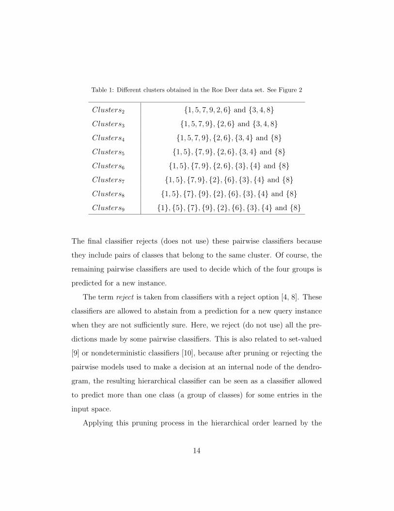
Table 1: Different clusters obtained in the Roe Deer data set. See Figure 2

Clusters2 {1, 5, 7, 9, 2, 6} and {3, 4, 8}

Clusters3 {1, 5, 7, 9}, {2, 6} and {3, 4, 8}

Clusters4 {1, 5, 7, 9}, {2, 6}, {3, 4} and {8}

Clusters5 {1, 5}, {7, 9}, {2, 6}, {3, 4} and {8}

Clusters6 {1, 5}, {7, 9}, {2, 6}, {3}, {4} and {8}

Clusters7 {1, 5}, {7, 9}, {2}, {6}, {3}, {4} and {8}

Clusters8 {1, 5}, {7}, {9}, {2}, {6}, {3}, {4} and {8}

Clusters9 {1}, {5}, {7}, {9}, {2}, {6}, {3}, {4} and {8}

The final classifier rejects (does not use) these pairwise classifiers because

they include pairs of classes that belong to the same cluster. Of course, the

remaining pairwise classifiers are used to decide which of the four groups is

predicted for a new instance.

The term reject is taken from classifiers with a reject option [4, 8]. These

classifiers are allowed to abstain from a prediction for a new query instance

when they are not sufficiently sure. Here, we reject (do not use) all the pre-

dictions made by some pairwise classifiers. This is also related to set-valued

[9] or nondeterministic classifiers [10], because after pruning or rejecting the

pairwise models used to make a decision at an internal node of the dendro-

gram, the resulting hierarchical classifier can be seen as a classifier allowed

to predict more than one class (a group of classes) for some entries in the

input space.

Applying this pruning process in the hierarchical order learned by the

14

hierarchical clustering, we have a bunch of classifiers, hk : X → Clustersk,

one for each partition of k clusters (see Table 1). In this case, we consider

an example to be classified correctly if the cluster thus predicted contains its

true class. We can accordingly obtain classification errors not only for the

original set of N classes, but also for k = N − 1, . . . , 2 number of clusters,

without learning any new model. Figure 3 shows the classification errors of

the hierarchical classifier learned from the hierarchical clustering depicted

in Figure 2 for every possible number of clusters. Obviously, if we consider

the 0/1 loss function, the classification error will decrease as we prune the

original hierarchical classifier (as k decreases).

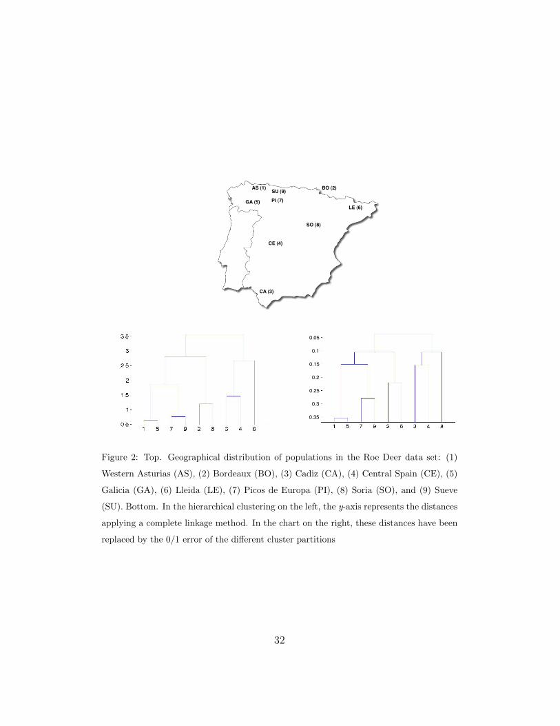
This set of 0/1 loss values obtained for each number of clusters can show

very useful information and can be a good replacement for the y-axis dis-

tances of the hierarchical clustering, which are sometimes difficult to inter-

pret. In a hierarchical clustering, the y-axis usually represents the distance

between clusters (see Figure 2, bottom-left). However, these distances are

often not very informative, as they can depend on the linkage method em-

ployed. In PSMT, these distances can be replaced by the 0/1 loss or the

accuracy obtained by the set of hk classifiers (see Figure 2, bottom-right).

The hierarchical clustering chart thus shows the user not only all the parti-

tions that can be made, but also how easy it is to discriminate between these

groups.

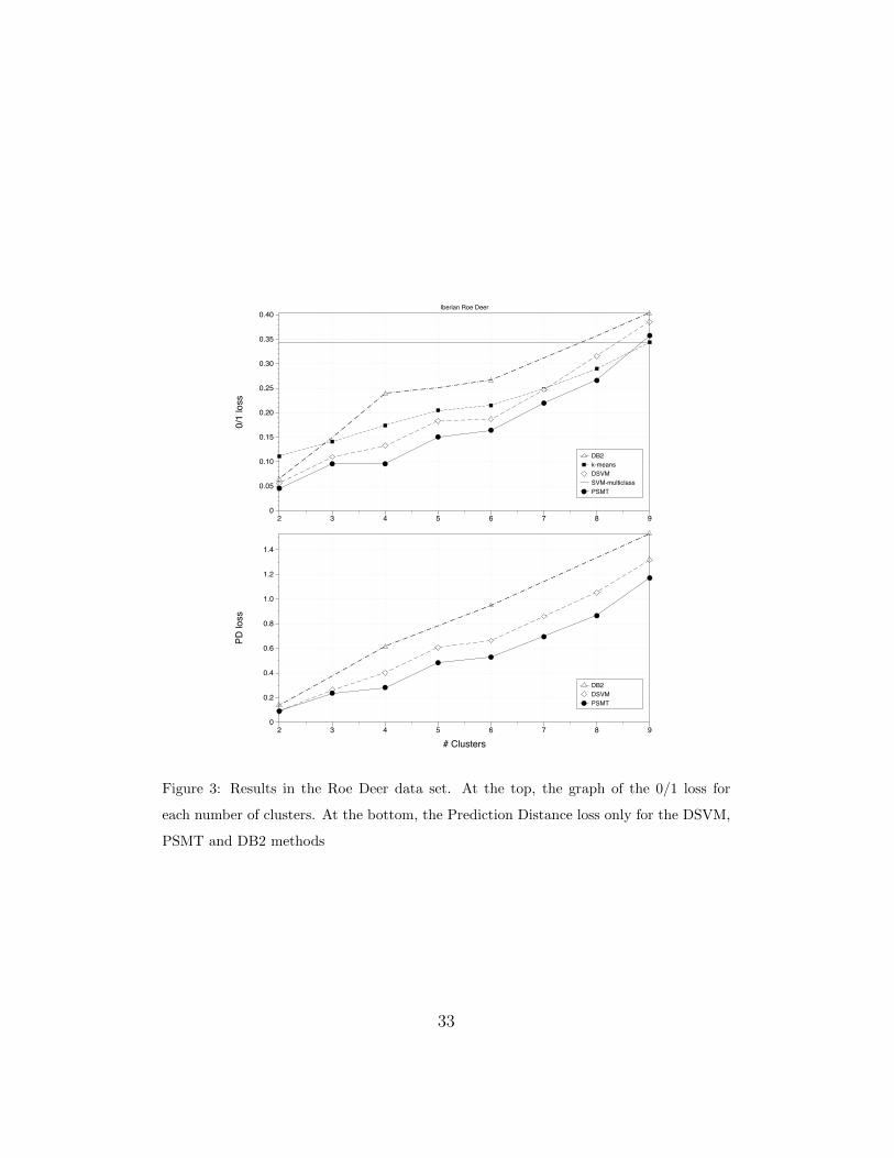
Analyzing the results of PSMT over the Roe Deer data set, also depicted

in Figure 3 (top), the 0/1 loss for 4 clusters is quite small (less than 10%)

and even for 6 clusters, the error is acceptable (around 15%). In fact, there is

only a small increase in the 0/1 error between 5 and 6 clusters. This means

15

that classes 3 and 4 are easy to distinguish. For more than 6 clusters, the

0/1 error increases almost linearly with the number of clusters. This means

that classes 1 and 5, 7 and 9, and 2 and 6 are very difficult to distinguish.

As they were sampled in close geographical or environmental areas, it is not

surprising that our hierarchical clustering (see Figure 2) identifies them as

those populations with the highest genetic identity.

Another kind of information that can be useful to study is what happens

when a hierarchical classifier fails. A hierarchical clustering of classes must

somehow represent the similarity between these classes. When the hierarchi-

cal classifier with k classes (hk) misclassifies an example ~xi, if the hierarchy is

good, the predicted group of classes hk(~xi) must be near (in the hierarchy) to

the node containing the true class yi. Therefore, we can compute the distance

in the hierarchy between predictions and true classes; i.e., the number of arcs

along the path between the nodes labeled by those classes in the dendrogram

T . This measure was originally presented in the Hieron method of Dekel et

al. [14] under the name of γ. In order to be more informative, we rename it

as the Prediction Distance (PD):

PD(hk(~xi), yi, T ) = #arcs(hk(~xi), yi, T ). (7)

For instance, considering the h8 classifier in Figure 1 and Figure 2, the PD

of an example from class 7 (see Figure 2) classified as the group of classes

{1, 5} is 3, but if the prediction were class 2, the PD would increase to 5.

The furthest classes from class 7 are 3 and 4, both a distance of 7. Note that

the maximum distance between two classes in a dendrogram of N classes is

N and the minimum is 2. Averaging this metric over the total number of

test examples, we shall measure the goodness of a hierarchy T .

16

4. Experimental results

This section has two main objectives. The first (see Section 4.1) is to

demonstrate that the PSMT algorithm is able to build meaningful hierarchi-

cal clusters of classes while improving the predictive power of SMT, thereby

producing more accurate results comparable to those obtained with one-vs-

one multi-class SVM. The second objective is to show how clustering-of-

classes algorithms can be used to deal with problems in which the main goal

is to discover relationships between the classes involved (see Section 4.2).

In order to test our method, we employed six different learning algo-

rithms in the experiments. Three of these represent classes by means of their

centroids, i.e.:

~µm =1

nm

∑∀~xi∈Cm

~xi, (8)

where nm is the number of data points in class Cm. We then tested different

methods able to solve multi-class tasks with or without a hierarchy:

• SVM. A multi-class support vector machine based on one-vs-one models

and the Max Wins [19] method to combine the output of binary models

in the classification stage.

• DSVM [5]. Dendrogram-based Support Vector Machines build a den-

drogram employing the distance between the different classes, which is

computed by means of the Euclidean distance between the centroids of

each pair of classes.

• k-means. We run the k-means algorithm with k = 2, . . . , N−1, employ-

ing the centroids of the classes. A multi-class SVM classifier is then

17

learned for each different group of clusters. We obtain classification

results from 2 to N − 1 clusters of populations.

• Divide-by-2 (DB2) [32]. This method recursively applies a k-means

algorithm (with k = 2) using the centroids of the classes to build a

binary tree with the set of classes at its leaves. In this case, we cannot

obtain N −1 different classifiers because this method does not produce

a hierarchical clustering. The learned binary tree can only be broken

up using the depth of its leaves. In line with the idea discussed in

Section 3, we thus obtain a variable number of classifiers that depends

on the topology of the tree.

• Soft Margin Trees (SMT) [16]. The hierarchy of classes is constructed

from the distance matrix computed by applying Equations 5 and 6. A

binary model is then learnt at each internal node of the hierarchy to

separate examples belonging to the two descending branches.

• Pairwise Soft Margin Trees (PSMT). The difference with respect to

SMT is that it is not necessary to learn a new model at each internal

node because the pairwise models learned to construct the hierarchy

are also used to build the hierarchical classifier (see Section 2.1).

All the reported scores were estimated by means of a five-fold cross vali-

dation repeated twice. We did not use the ten-fold procedure, as in certain

data sets there are too few examples in some classes. The SVM implemen-

tation used was libsvm [33], with the linear kernel for all methods. For each

hierarchical classifier, DSVM, DB2 and SMT, we used the same regulariza-

tion parameter C in all models learned at each node in the tree. In the case

18

of k-means classifiers, we used a different value of C for each of them. In

all cases, we employed a two-fold cross validation (using only training data)

repeated five times, searching within C ∈ [10−2, . . . , 102] to select this param-

eter. The aim in this grid search was to optimize the 0/1 loss of the original

multi-class task. We report the error rate of these classifiers in addition to

the prediction distance (PD) (Equation 7). Although the quality of the trees

can be measured only by means of the Prediction Distance, we include the

0/1 los so as to compare their performance as classifiers with the multi-class

SVM.

4.1. Comparison with other algorithms

We conducted a battery of experiments to analyze the improvement that

the pairwise methodology (see Section 2.1) contributes to the idea presented

in the SMT algorithm. The aim was to show that the PSMT algorithm is

able to produce accurate results comparable to those obtained with SVM

employing only the pairwise models learned in the construction of the hier-

archy.

The data sets used in the experiments are described in Table 2. There are

data sets with a greater number of examples than features, and vice versa.

The first group is formed by data sets obtained from the UCI repository [2].

We selected those data sets that fulfill the following rules: continuous or

ordinal attribute values, no more than 40 attributes, no more than 10000

examples, while excluding data sets with missing values and with less than

4 classes. The second group is composed of the data sets used in [30]. These

comprise 7 data sets whose goal is to classify cancer patients from gene

expressions captured by microarrays.

19

No results of k-means are shown as in this experiment we try to learn to

distinguish all the classes (multi-class task) without grouping any of them.

Following [15], a two-step statistical test procedure was carried out. The

first step consists of a Friedman test of the null hypothesis that all approaches

perform equally. In the case of this hypothesis being rejected, a Nemenyi

test is then conducted to compare the methods in a pairwise way. Both tests

are based on the average of the ranks. The 0/1 loss comparison includes 5

algorithms over 18 data sets; so the critical difference (CD) at a significance

level of 10% in the Nemenyi test is 1.2960. In the PD comparison, only 4

algorithms were tested over the same data sets; in this case, the CD at the

same significance level is 0.9859.

Table 3 shows the 0/1 loss results obtained in the experiments. As can be

seen, SVM is the best method and DB2 is the worst, whereas PSMT produces

error rates comparable to those obtained by SVM. DSVM and SMT provide

similar results. To analyze the results in more depth, the Friedman test

suggests that there are significant differences between the methods, while

the Nemenyi test indicates that SVM is significantly better than the other

algorithms, except for PSMT (see Figure 4, top). No significant differences

can be observed, however, between DB2, DVSM and SMT.

As mentioned previously, the quality of the hierarchies can be measured

by the PD. We can see from Table 4 that PSMT achieves the best results,

followed by SMT. DB2 and DSVM perform worse, so the distance in the

hierarchy between predictions and the true class is bigger. In this case, the

Nemenyi test shows us that PSMT is significantly better than DSVM and

DB2 (see Figure 4, bottom).

20

4.2. Population Genetics Applications

The aim of this section is to show that our approach (PSMT) is able

to build meaningful hierarchical clusters of classes which are better than

those obtained by other approaches and that it can be very useful to solve

population genetics applications. We devote one section to each of the three

applications addressed in this paper. We shall describe the main results and

draw some useful conclusions for these applications.

In this experiment, we used all the clustering algorithms presented pre-

viously except SMT, because, as was shown in the previous section, PSMT

obtains the same hierarchical clusterings, but better classifiers. The goal is to

compare very different approaches: a clustering method without any struc-

ture (k-means), a top-down binary tree (DB2), a centroids-based hierarchical

clustering (DSVM) and a pairwise-based hierarchical clustering (PSMT).

As we wish to explain the results obtained by the hierarchical classifiers

learned by PSMT using concrete dendrograms of classes, first of all the clus-

tering of classes is obtained for all the methods considered using the complete

data set of examples. We then estimate the different classification errors (0/1

loss and PD, except for k-means, as it is not applicable) by means of a five-

fold cross-validation repeated twice. If we had included the construction of

the clustering in the cross-validation process, the clusterings could be dif-

ferent in each execution. Therefore, the classification errors thus obtained

would not correspond to a particular clustering. Although this could be seen

as an optimistic estimation, other experiments carried out showed that both

methods produced almost identical results. In any case, all the algorithms

considered use the same procedure.

21

4.2.1. Iberian Roe Deer (Capreolus capreolus)

Royo et al., see [29], studied 109 Iberian roe deer individuals correspond-

ing to 9 Spanish populations. Individuals were sampled at locations that

were expected to have acted as refugia for the species during the decrease

in population size in the 20th century. Samples were analyzed by means

of 10 microsatellites. Using these microsatellites, correspondence analysis

and molecular coancestry information revealed high molecular differentiation

among Northwestern ({1, 5, 7, 9}) and Central-Southern ({3, 4, 8}) Spanish

roe deer populations, with two Pyrenean populations ({2, 6}) being charac-

terized as non-local, reintroduced populations.

Analyzing the hierarchical clustering obtained by PSMT (Figure 2) it

seems clear that there are two main groups corresponding to the two main

regions described in [29]. The left cluster {1, 5, 7, 9, 2, 6} corresponds to

Northwestern populations (with a further subdivision including the Pyre-

nean populations: 2 and 6), while the right cluster {3, 4, 8} is formed by

Central-Southern populations. In this case, the clustering obtained is almost

geographical, but well explained according to the between-populations ge-

netic identities found in the original genetic study cited previously. In fact,

the classifier for these two groups has a low 0/1 loss, considering that the

original task is quite difficult.

Figure 3 shows the performance of the different algorithms when the

number of clusters increases. It can be seen that with 4 clusters, PSMT

obtains acceptable results: less than 11% in 0/1 loss and less than 0.3 in PD.

The clusters are the following: i) {1, 5, 7, 9} includes Northwestern roe deer,

ii) {2, 6} animals from the Pyrenees area, iii) {3, 4} Southern populations,

22

and iv) {8} animals from the Iberian branch.

4.2.2. Eurasian Otter (Lutra lutra) in Britain

In [13], the authors assessed the effects of gene flow and population frag-

mentation on the genetic structure in British populations of the Eurasian

otter. The analysis was based on genotypes consisting of 12 microsatellites

from 618 individuals belonging to 17 different populations. The main goal of

the paper was to compare the genetic makeup of the continuous otter pop-

ulation in Scotland with respect those in Wales and South West England.

Otters in southern Britain contained significantly lower levels of microsatel-

lite polymorphism than otters in Scotland, and the population in the western

peninsula of SW England was genetically distinct. Interestingly, the Scot-

tish otter population showed a significant genetic structure (Northern Isles,

North Scotland and South Scotland), which was more likely due to restricted

contemporary gene flow than to historical fluctuations in the size of subpop-

ulations.

Figure 5 shows the hierarchical clustering obtained by PSMT and the

geographical layout of the different populations. It can be seen that the al-

gorithm obtains a geographically coherent hierarchy, creating groups with

otters from the Northern Isles, North Scotland, South Scotland, Wales and

SW England. At first sight, it may seem strange that ORK, a Northern Isles

population, appears close to Welsh populations, but this is not so strange

given that [13] showed that there are no significant differences in levels of

microsatellite polymorphism between these populations. Although the con-

nection between this pair of breeds is supported by the bibliography, we can

appreciate that this connection is produced at a high distance. A similar sit-

23

uation occurs with STR, a North Scotland population, which is placed close

to South Scotland populations; once again, significant differences were not

found between these populations in [13]. However, in this case our method

assesses a lower distance to the node separating the STR and the South

Scotland otter populations. The lack of differences between STR and the

other members of its cluster may be explained by a continuous between-

populations gene flow in the area of the source of the rivers flowing to these

areas. Once more, our method automatically obtains a hierarchical clustering

that is supported by previous studies in the field of population genetics.

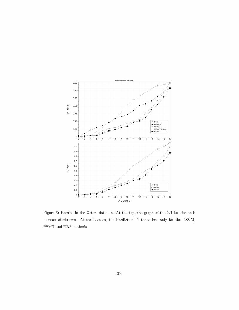
An analysis of how the algorithms perform when the number of clus-

ters is increased can be seen in Figure 6. With 5 clusters, we obtain 1% in

0/1 loss and 0.03 in PD. The clusters are the following: i) {1, 2, 3} Shet-

land populations; ii) {4} Orkney otters; iii) {14, 15} Wales populations; iv)

{5, 6, 7, 8, 9, 10, 11, 12, 13} Scotland populations; and v) {16, 17} SW Eng-

land otters. If we wish to descend one step in the hierarchy, we will have to

split the fourth cluster in two: {5, 6, 7, 8, 9} North Scotland populations, and

{10, 11, 12, 13} South Scotland population plus STR. With these 6 clusters,

the 0/1 loss increases to 2.5% and the PD to 0.07.

4.2.3. African Cattle Structure

Hanotte et al., see [20], genotyped 15 microsatellite loci on 50 local African

cattle breeds fully representative of present-day African cattle stock (mainly

populations with a different admixture of B. taurus and B. indicus, known

as ’sanga’), and on 5 European B. taurus and 3 Asian B. indicus cattle

breeds, used as outgroups, in order to ascertain the genetic signatures of

their origins, spread and differentiation. The hypotheses tested were: a) an

24

expansion of the ’original’ West African cattle southwards (which occurred

during the pastoralist migrations of the Middle Ages that eventually invaded

present-day South Africa); b) an intense B. indicus introgression into the

’original’ African taurine cattle from the Horn and the East Coast of Africa

to Sub-Saharan West Africa and to South Africa via Tanzania and Malawi;

and c) a recent genetic influence of European B. taurus cattle.

The hierarchy obtained by the PSMT algorithm is presented in Figure 7.

To analyze the hierarchy, we break up the hierarchical clustering to obtain

5 groups of populations. From left to right, the first group is composed of

{56, 57, 58} Asian breeds, all of which are B. indicus. The second group

contains 27 breeds: 17 B. indicus and 10 B. taurus. This coincides with

the findings by [20], as these 10 B. taurus breeds have the highest estimated

proportion of Asian zebu admixture (see Supplementary Data in [20]). The

third group has 2 B. indicus and 16 B. taurus breeds. According to the

Supplementary Data in [20], the two B. indicus breeds have the lowest esti-

mated proportion of Asian zebu admixture. The fourth group is composed

of {11, 46, 36, 22, 35} breeds, all of which are B. taurus. Finally, the last

group contains {13, 53, 52, 54, 55} breeds, namely four European breeds and

the Moroccan Blonde breed (highly influenced by European cattle), all of

which are B. taurus.

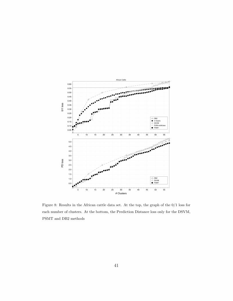
Figure 8 shows the performance of the algorithms when the number of

clusters increases. It can be seen that, for 5 clusters, the PSMT obtains 12.6%

of 0/1 loss and 0.53 of PD. The higher the number of clusters assumed, the

higher the between-algorithms differences in performance.

25

5. Conclusions

We have developed a new methodology to deal with data in the field of

population genetics. Starting from the genetic description of a set of individ-

uals belonging to a limited number of populations (e.g. different species or

breeds), our system, PSMT, is able to produce: 1) a hierarchical clustering

of populations; and 2) a model for a hierarchical classification of individu-

als. Both the hierarchical clustering and the classifier can be broken up at

different levels to yield different clusterings of the set of classes and different

classifiers. We have shown the usefulness of PSMT, presenting the exper-

imental results achieved with three interesting applications in the field of

population genetics.

The paper also presents a new method for the classification stage of the

hierarchical model in a multi-class learning task. This method is faster than

the previous one and obtains better results in the data sets used in the

experiments: 11 UCI data sets and 7 data sets whose goal is to classify

cancer patients from gene expressions captured by microarrays. We compare

our algorithm with 5 other algorithms, concluding that PSMT performs well

both as a multi-class classifier and as a clustering algorithm. Moreover, the

proposed method is computationally as efficient as the well-known one-vs-one

multi-class SVM.

Acknowledgements

The authors are indebted to Dr. Olivier Hanotte for kindly providing

the African cattle genetic dataset used in this work. This research has been

26

partially supported by Spanish Ministerio de Ciencia e Innovacion (MICINN)

grants TIN2008-06247 and TIN2011-23558.

References

[1] A. Ahmadi, S. Omatu, T. Fujinaka, T. Kosaka, Improvement of relia-

bility in banknote classification using reject option and local pca, Infor-

mation Sciences 168 (2004) 277 – 293.

[2] A. Asuncion, D. Newman, UCI machine learning repository, School of

Information and Computer Sciences. University of California, Irvine,

California, USA (2007).

[3] R.C. Barros, D.D. Ruiz, M.P. Basgalupp, Evolutionary model trees for

handling continuous classes in machine learning, Information Sciences

181 (2011) 954–971.

[4] P. Bartlett, M. Wegkamp, Classification with a reject option using a

hinge loss, Journal of Machine Learning Research 9 (2008) 1823–1840.

[5] K. Benabdeslem, Y. Bennani, Dendogram based svm for multi-class clas-

sification, Journal of Computing and Information Technology 14 (2006)

283–289.

[6] B.E. Boser, I. Guyon, V. Vapnik, A training algorithm for optimal mar-

gin classifiers, in: Computational Learing Theory, pp. 144–152.

[7] N. Cesa-Bianchi, C. Gentile, L. Zaniboni, Incremental algorithms for hi-

erarchical classification, Journal of Machine Learning Research 7 (2006)

31–54.

27

[8] C. Chow, On optimum recognition error and reject tradeoff, IEEE Trans-

actions on Information Theory 16 (1970) 41–46.

[9] G. Corani, M. Zaffalon, Learning reliable classifiers from small or in-

complete data sets: the naıve credal classifier 2, Journal of Machine

Learning Research 9 (2008) 581–621.

[10] J.J. del Coz, J. Dıez, A. Bahamonde, Learning nondeterministic classi-

fiers, Journal of Machine Learning Research 10 (2009) 2273–2293.

[11] K. Crammer, Y. Singer, On the algorithmic implementation of multiclass

kernel-based vector machines, Journal of Machine Learning Research 2

(2001) 265–292.

[12] N. Cristianini, J. Shawe-Taylor, An Introduction to Support Vector Ma-

chines and other kernel-based learning methods, Cambridge University

Press, 2000.

[13] J. Dallas, F. Marshall, S. Piertney, P. Bacon, P. Racey, Spatially

restricted gene flow and reduced microsatellite polymorphism in the

eurasian otter lutra lutra in britain, Conservation Genetics 3 (2002)

15–29.

[14] O. Dekel, J. Keshet, Y. Singer, Large margin hierarchical classification,

in: Proceedings of the 21st International Conference on Machine learn-

ing, pp. 209–216.

[15] J. Demsar, Statistical Comparisons of Classifiers over Multiple Data

Sets, Journal of Machine Learning Research 7 (2006) 1–30.

28

[16] J. Dıez, J. Coz, A. Bahamonde, O. Luaces, Soft margin trees, in: Eu-

ropean Conference on Machine Learning and Principles and Practice of

Knowledge Discovery in Databases (ECML PKDD ’09), Springer-Verlag,

2009, pp. 302–314.

[17] J. Dıez, J.J. del Coz, A. Bahamonde, A semi-dependent decomposition

approach to learn hierarchical classifiers, Pattern Recognition 43 (2010)

3795–3804.

[18] A.A. Freitas, D.C. Wieser, R. Apweiler, On the importance of

comprehensible classification models for protein function prediction,

IEEE/ACM Trans. Comput. Biol. Bioinformatics 7 (2010) 172–182.

[19] J. Friedman, Another approach to polychotomous classification, Tech-

nical Report, Department of Statistics, Stanford University, 1996.

[20] O. Hanotte, D.G. Bradley, J.W. Ochieng, Y. Verjee, E.W. Hill, J.E.O.

Rege, African Pastoralism: Genetic Imprints of Origins and Migrations,

Science 296 (2002) 336–339.

[21] J.A. Hartigan, Clustering Algorithms, John Wiley & Sons, Inc., New

York, NY, USA, 1975.

[22] C.C. Hsu, C.L. Chen, Y.W. Su, Hierarchical clustering of mixed data

based on distance hierarchy, Information Sciences 177 (2007) 4474 –

4492.

[23] J. Huysmans, K. Dejaeger, C. Mues, J. Vanthienen, B. Baesens, An

empirical evaluation of the comprehensibility of decision table, tree and

29

rule based predictive models, Decision Support Systems 51 (2011) 141–

154.

[24] U. Kreßel, Pairwise classification and support vector machines, in:

B. Scholkopf, C.J.C. Burges, A.J. Smola (Eds.), Advances in Kernel

Methods – Support Vector Learning, MIT Press, Cambridge, MA, 1999,

pp. 255–268.

[25] J.Z. Lai, T.J. Huang, An agglomerative clustering algorithm using a

dynamic k-nearest-neighbor list, Information Sciences 181 (2011) 1722

– 1734.

[26] H. Lei, V. Govindaraju, Half-against-half multi-class support vector ma-

chines, in: 6th International Workshop on Multiple Classifier Systems,

Springer, 2005, pp. 156–164.

[27] J.K. Pritchard, M. Stephens, P. Donnelly, Inference of population struc-

ture using multilocus genotype data, Genetics 155 (2000) 945–959.

[28] J. Rousu, C. Saunders, S. Szedmak, J. Shawe-Taylor, Kernel-based

learning of hierarchical multilabel classification models, Journal of Ma-

chine Learning Research 7 (2006) 1601–1626.

[29] L.J. Royo, G. Pajares, I. Alvarez, I. Fernandez, F. Goyache, Genetic vari-

ability and differentiation in spanish roe deer (capreolus capreolus): A

phylogeographic reassessment within the european framenwork, Molec-

ular Phylogenetics and Evolution 42 (2007) 47–61.

[30] R. Tibshirani, T. Hastie, Margin Trees for High-dimensional Classifica-

tion, Journal of Machine Learning Research 8 (2007) 637–652.

30

[31] V. Vapnik, Statistical Learning Theory, John Wiley, New York, NY,

1998.

[32] V. Vural, J.G. Dy, A hierarchical method for multi-class support vector

machines, in: ICML ’04: Proceedings of the twenty-first international

conference on Machine learning, ACM, New York, NY, USA, 2004, pp.

105–112.

[33] T. Wu, C. Lin, R. Weng, Probability Estimates for Multi-class Classi-

fication by Pairwise Coupling, Journal of Machine Learning Research 5

(2004) 975–1005.

[34] C. Zhong, D. Miao, P. Franti, Minimum spanning tree based split-

and-merge: A hierarchical clustering method, Information Sciences 181

(2011) 3397 – 3410.

31

AS (1) SU (9)

GA (5) PI (7)

CE (4)

CA (3)

SO (8)

LE (6)

BO (2)

0.05

0.1

0.15

0.2

0.25

0.3

0.35

Figure 2: Top. Geographical distribution of populations in the Roe Deer data set: (1)

Western Asturias (AS), (2) Bordeaux (BO), (3) Cadiz (CA), (4) Central Spain (CE), (5)

Galicia (GA), (6) Lleida (LE), (7) Picos de Europa (PI), (8) Soria (SO), and (9) Sueve

(SU). Bottom. In the hierarchical clustering on the left, the y-axis represents the distances

applying a complete linkage method. In the chart on the right, these distances have been

replaced by the 0/1 error of the different cluster partitions

32

0/1

loss

0

0.05

0.10

0.15

0.20

0.25

0.30

0.35

0.40

2 3 4 5 6 7 8 9

Iberian Roe Deer

DB2k-meansDSVMSVM-multiclassPSMT

PD lo

ss

0

0.2

0.4

0.6

0.8

1.0

1.2

1.4

# Clusters2 3 4 5 6 7 8 9

DB2DSVMPSMT

Figure 3: Results in the Roe Deer data set. At the top, the graph of the 0/1 loss for

each number of clusters. At the bottom, the Prediction Distance loss only for the DSVM,

PSMT and DB2 methods

33

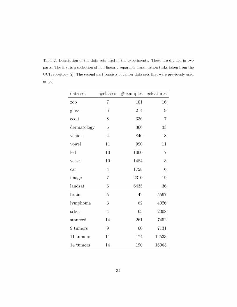
Table 2: Description of the data sets used in the experiments. These are divided in two

parts. The first is a collection of non-linearly separable classification tasks taken from the

UCI repository [2]. The second part consists of cancer data sets that were previously used

in [30]

data set #classes #examples #features

zoo 7 101 16

glass 6 214 9

ecoli 8 336 7

dermatology 6 366 33

vehicle 4 846 18

vowel 11 990 11

led 10 1000 7

yeast 10 1484 8

car 4 1728 6

image 7 2310 19

landsat 6 6435 36

brain 5 42 5597

lymphoma 3 62 4026

srbct 4 63 2308

stanford 14 261 7452

9 tumors 9 60 7131

11 tumors 11 174 12533

14 tumors 14 190 16063

34

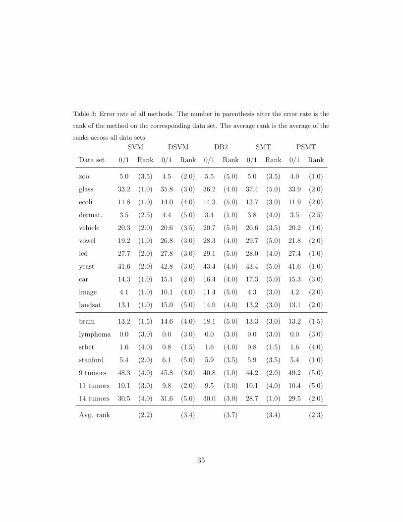
Table 3: Error rate of all methods. The number in parenthesis after the error rate is the

rank of the method on the corresponding data set. The average rank is the average of the

ranks across all data sets

SVM DSVM DB2 SMT PSMT

Data set 0/1 Rank 0/1 Rank 0/1 Rank 0/1 Rank 0/1 Rank

zoo 5.0 (3.5) 4.5 (2.0) 5.5 (5.0) 5.0 (3.5) 4.0 (1.0)

glass 33.2 (1.0) 35.8 (3.0) 36.2 (4.0) 37.4 (5.0) 33.9 (2.0)

ecoli 11.8 (1.0) 14.0 (4.0) 14.3 (5.0) 13.7 (3.0) 11.9 (2.0)

dermat. 3.5 (2.5) 4.4 (5.0) 3.4 (1.0) 3.8 (4.0) 3.5 (2.5)

vehicle 20.3 (2.0) 20.6 (3.5) 20.7 (5.0) 20.6 (3.5) 20.2 (1.0)

vowel 19.2 (1.0) 26.8 (3.0) 28.3 (4.0) 29.7 (5.0) 21.8 (2.0)

led 27.7 (2.0) 27.8 (3.0) 29.1 (5.0) 28.0 (4.0) 27.4 (1.0)

yeast 41.6 (2.0) 42.8 (3.0) 43.4 (4.0) 43.4 (5.0) 41.6 (1.0)

car 14.3 (1.0) 15.1 (2.0) 16.4 (4.0) 17.3 (5.0) 15.3 (3.0)

image 4.1 (1.0) 10.1 (4.0) 11.4 (5.0) 4.3 (3.0) 4.2 (2.0)

landsat 13.1 (1.0) 15.0 (5.0) 14.9 (4.0) 13.2 (3.0) 13.1 (2.0)

brain 13.2 (1.5) 14.6 (4.0) 18.1 (5.0) 13.3 (3.0) 13.2 (1.5)

lymphoma 0.0 (3.0) 0.0 (3.0) 0.0 (3.0) 0.0 (3.0) 0.0 (3.0)

srbct 1.6 (4.0) 0.8 (1.5) 1.6 (4.0) 0.8 (1.5) 1.6 (4.0)

stanford 5.4 (2.0) 6.1 (5.0) 5.9 (3.5) 5.9 (3.5) 5.4 (1.0)

9 tumors 48.3 (4.0) 45.8 (3.0) 40.8 (1.0) 44.2 (2.0) 49.2 (5.0)

11 tumors 10.1 (3.0) 9.8 (2.0) 9.5 (1.0) 10.1 (4.0) 10.4 (5.0)

14 tumors 30.5 (4.0) 31.6 (5.0) 30.0 (3.0) 28.7 (1.0) 29.5 (2.0)

Avg. rank (2.2) (3.4) (3.7) (3.4) (2.3)

35

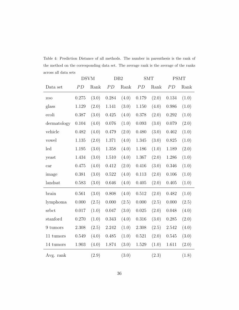
Table 4: Prediction Distance of all methods. The number in parenthesis is the rank of

the method on the corresponding data set. The average rank is the average of the ranks

across all data sets

DSVM DB2 SMT PSMT

Data set PD Rank PD Rank PD Rank PD Rank

zoo 0.275 (3.0) 0.284 (4.0) 0.179 (2.0) 0.134 (1.0)

glass 1.129 (2.0) 1.141 (3.0) 1.150 (4.0) 0.986 (1.0)

ecoli 0.387 (3.0) 0.425 (4.0) 0.378 (2.0) 0.292 (1.0)

dermatology 0.104 (4.0) 0.076 (1.0) 0.093 (3.0) 0.079 (2.0)

vehicle 0.482 (4.0) 0.479 (2.0) 0.480 (3.0) 0.462 (1.0)

vowel 1.135 (2.0) 1.371 (4.0) 1.345 (3.0) 0.825 (1.0)

led 1.195 (3.0) 1.358 (4.0) 1.186 (1.0) 1.189 (2.0)

yeast 1.434 (3.0) 1.510 (4.0) 1.367 (2.0) 1.286 (1.0)

car 0.475 (4.0) 0.412 (2.0) 0.416 (3.0) 0.346 (1.0)

image 0.381 (3.0) 0.522 (4.0) 0.113 (2.0) 0.106 (1.0)

landsat 0.583 (3.0) 0.646 (4.0) 0.405 (2.0) 0.405 (1.0)

brain 0.561 (3.0) 0.808 (4.0) 0.512 (2.0) 0.482 (1.0)

lymphoma 0.000 (2.5) 0.000 (2.5) 0.000 (2.5) 0.000 (2.5)

srbct 0.017 (1.0) 0.047 (3.0) 0.025 (2.0) 0.048 (4.0)

stanford 0.270 (1.0) 0.343 (4.0) 0.316 (3.0) 0.285 (2.0)

9 tumors 2.308 (2.5) 2.242 (1.0) 2.308 (2.5) 2.542 (4.0)

11 tumors 0.549 (4.0) 0.485 (1.0) 0.521 (2.0) 0.545 (3.0)

14 tumors 1.903 (4.0) 1.874 (3.0) 1.529 (1.0) 1.611 (2.0)

Avg. rank (2.9) (3.0) (2.3) (1.8)

36

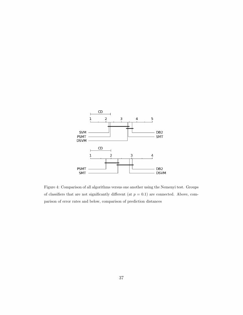
Figure 4: Comparison of all algorithms versus one another using the Nemenyi test. Groups

of classifiers that are not significantly different (at p = 0.1) are connected. Above, com-

parison of error rates and below, comparison of prediction distances

37

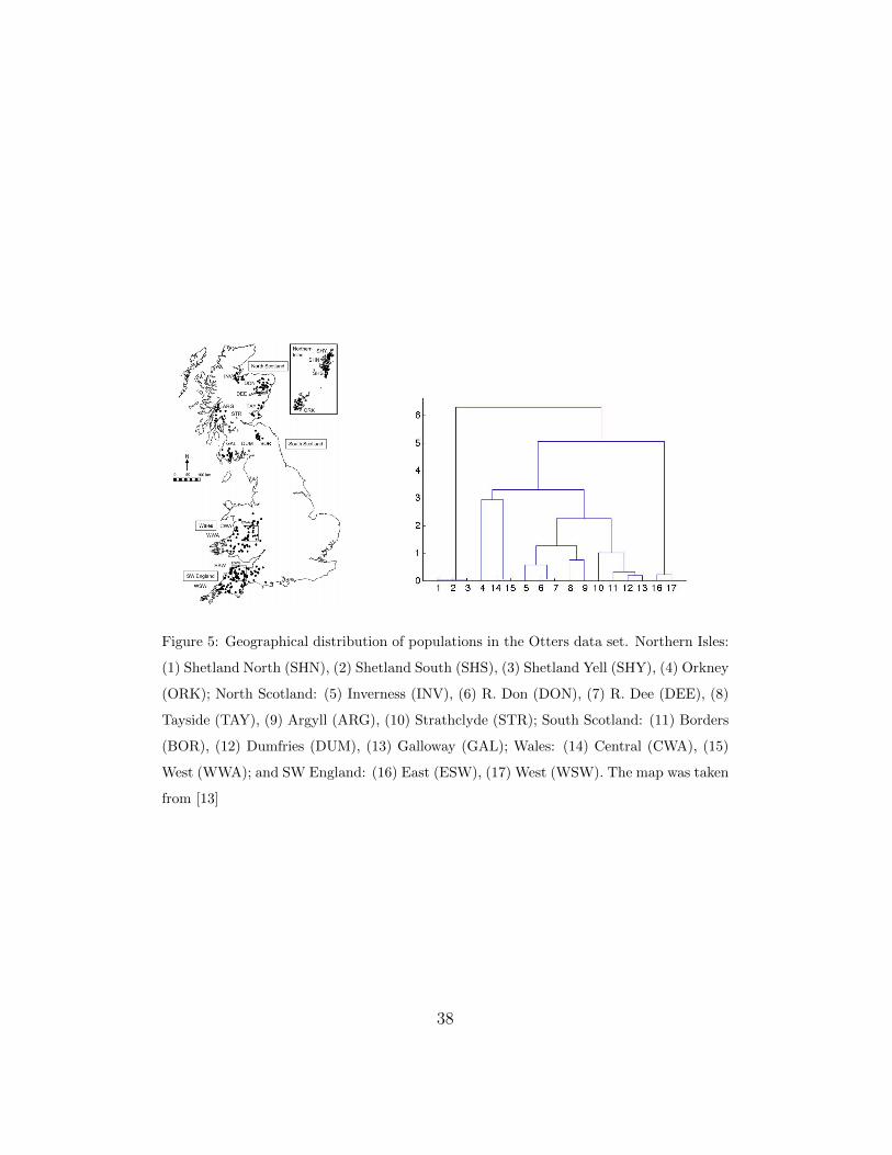
Figure 5: Geographical distribution of populations in the Otters data set. Northern Isles:

(1) Shetland North (SHN), (2) Shetland South (SHS), (3) Shetland Yell (SHY), (4) Orkney

(ORK); North Scotland: (5) Inverness (INV), (6) R. Don (DON), (7) R. Dee (DEE), (8)

Tayside (TAY), (9) Argyll (ARG), (10) Strathclyde (STR); South Scotland: (11) Borders

(BOR), (12) Dumfries (DUM), (13) Galloway (GAL); Wales: (14) Central (CWA), (15)

West (WWA); and SW England: (16) East (ESW), (17) West (WSW). The map was taken

from [13]

38

0/1

loss

0

0.05

0.10

0.15

0.20

0.25

0.30

0.35

2 3 4 5 6 7 8 9 10 11 12 13 14 15 16 17

Eurasian Otter in Britain

DB2k-meansDSVMSVM-multiclassPSMT

PD lo

ss

0

0.1

0.2

0.3

0.4

0.5

0.6

0.7

0.8

0.9

1.0

# Clusters2 3 4 5 6 7 8 9 10 11 12 13 14 15 16 17

DB2DSVMPSMT

Figure 6: Results in the Otters data set. At the top, the graph of the 0/1 loss for each

number of clusters. At the bottom, the Prediction Distance loss only for the DSVM,

PSMT and DB2 methods

39

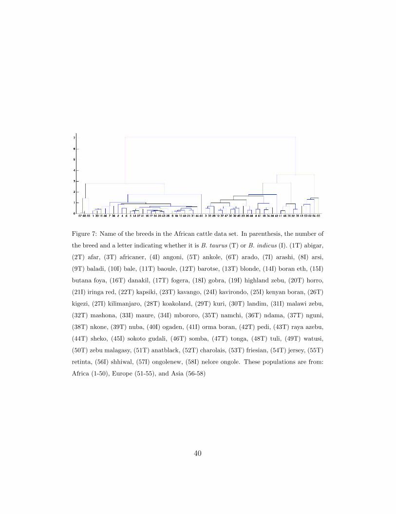
Figure 7: Name of the breeds in the African cattle data set. In parenthesis, the number of

the breed and a letter indicating whether it is B. taurus (T) or B. indicus (I). (1T) abigar,

(2T) afar, (3T) africaner, (4I) angoni, (5T) ankole, (6T) arado, (7I) arashi, (8I) arsi,

(9T) baladi, (10I) bale, (11T) baoule, (12T) barotse, (13T) blonde, (14I) boran eth, (15I)

butana foya, (16T) danakil, (17T) fogera, (18I) gobra, (19I) highland zebu, (20T) horro,

(21I) iringa red, (22T) kapsiki, (23T) kavango, (24I) kavirondo, (25I) kenyan boran, (26T)

kigezi, (27I) kilimanjaro, (28T) koakoland, (29T) kuri, (30T) landim, (31I) malawi zebu,

(32T) mashona, (33I) maure, (34I) mbororo, (35T) namchi, (36T) ndama, (37T) nguni,

(38T) nkone, (39T) nuba, (40I) ogaden, (41I) orma boran, (42T) pedi, (43T) raya azebu,

(44T) sheko, (45I) sokoto gudali, (46T) somba, (47T) tonga, (48T) tuli, (49T) watusi,

(50T) zebu malagasy, (51T) anatblack, (52T) charolais, (53T) friesian, (54T) jersey, (55T)

retinta, (56I) shhiwal, (57I) ongolenew, (58I) nelore ongole. These populations are from:

Africa (1-50), Europe (51-55), and Asia (56-58)

40

0/1

loss

0.05

0.10

0.15

0.20

0.25

0.30

0.35

0.40

0.45

0.50

0.55

0.60

5 10 15 20 25 30 35 40 45 50 55

African Cattle

DB2k-meansDSVMSVM-multiclassPSMT

PD lo

ss

0.5

1.0

1.5

2.0

2.5

3.0

3.5

4.0

4.5

5.0

# Clusters5 10 15 20 25 30 35 40 45 50 55

DB2DSVMPSMT

Figure 8: Results in the African cattle data set. At the top, the graph of the 0/1 loss for

each number of clusters. At the bottom, the Prediction Distance loss only for the DSVM,

PSMT and DB2 methods

41