Learning Deep Architectures via Generalized Whitened Neural Networks

Ping Luo 1 2

Abstract

Whitened Neural Network (WNN) is a recentadvanced deep architecture, which improves con-vergence and generalization of canonical neuralnetworks by whitening their internal hidden rep-resentation. However, the whitening transforma-tion increases computation time. Unlike WNNthat reduced runtime by performing whiteningevery thousand iterations, which degeneratesconvergence due to the ill conditioning, wepresent generalized WNN (GWNN), which hasthree appealing properties. First, GWNN isable to learn compact representation to reducecomputations. Second, it enables whiteningtransformation to be performed in a short period,preserving good conditioning. Third, we proposea data-independent estimation of the covariancematrix to further improve computational efficien-cy. Extensive experiments on various datasetsdemonstrate the benefits of GWNN.

1. IntroductionDeep neural networks (DNNs) have improved perfor-mances of many applications, as the non-linearity of DNNsprovides expressive modeling capacity, but it also makesDNNs difficult to train and easy to overfit the training data.

Whitened neural network (WNN) (Desjardins et al., 2015),a recent advanced deep architecture, is ideally to solve theabove difficulties. WNN extends batch normalization (BN)(Ioffe & Szegedy, 2015) by normalizing the internal hiddenrepresentation using whitening transformation instead ofstandardization. Whitening helps regularize each diagonalblock of the Fisher Information Matrix (FIM) to be an

1Guangdong Provincial Key Laboratory of Computer Vi-sion and Virtual Reality Technology, Shenzhen Institutes ofAdvanced Technology, Chinese Academy of Sciences, Shen-zhen, China 2Multimedia Laboratory, The Chinese Universityof Hong Kong, Hong Kong. Correspondence to: Ping Luo<pluo@ie.cuhk.edu.hk>.

Proceedings of the 34 th International Conference on MachineLearning, Sydney, Australia, PMLR 70, 2017. Copyright 2017by the author(s).

approximation of the identity matrix. This is an appeal-ing property, as training WNN using stochastic gradientdescent (SGD) mimics the fast convergence of naturalgradient descent (NGD) (Amari & Nagaoka, 2000). Thewhitening transformation also improves generalization. Asdemonstrated in (Desjardins et al., 2015), WNN exhib-ited superiority when being applied to various networkarchitectures, such as autoencoder and convolutional neuralnetwork, outperforming many previous works includingSGD, RMSprop (Tieleman & Hinton, 2012), and BN.

Although WNN is able to reduce the number of trainingiterations and improve generalization, it comes with a priceof increasing training time, because eigen-decompositionoccupies large computations. The runtime scales up whenthe number of hidden layers that require whitening trans-formation increases. We revisit WNN by breaking downits performance and show that its main runtime comesfrom two aspects, 1) computing full covariance matrixfor whitening and 2) solving singular value decomposition(SVD). Previous work (Desjardins et al., 2015) suggests toovercome these problems by a) using a subset of trainingdata to estimate the full covariance matrix and b) solvingthe SVD every hundreds or thousands of training iterations.Both of them rely on the assumption that the SVD holds inthis period, but it is generally not true. When this periodbecomes large, WNN degenerates to canonical SGD due toill conditioning of FIM.

We propose generalized WNN (GWNN), which possessesthe beneficial properties of WNN, but significantly reducesits runtime and improves its generalization. We introducetwo variants of GWNN, including pre-whitening and post-whitening GWNNs. The former one whitens a hiddenlayer’s input values, whilst the latter one whitens the pre-activation values (hidden features). GWNN has three ap-pealing characteristics. First, compared to WNN, GWNNis capable of learning more compact hidden representa-tion, such that the SVD can be approximated by a fewtop eigenvectors to reduce computation. This compactrepresentation also improves generalization. Second, itenables the whitening transformation to be performed ina short period, maintaining conditioning of FIM. Third,by exploiting knowledge of the distribution of the hiddenfeatures, we calculate the covariance matrix in an analyticalform to further improve computational efficiency.

Generalized Whitened Neural Network

oi-1 oiWi oi-1 Pi-1

hi

oi-1 Pioi-1 Pi-1

hi

(a) fully-connected layer (fc) (b) whitened fc layer of WNN (c) pre-whitening GWNN (d) post-whitening GWNN

Wi WiWi

relu

bn

ϕi

oioi oioioioiˆ ˆ

ϕiϕi

ϕiϕi

ϕiϕioi-1～oi-1～

oi-1～oi-1～

ˆ ˆhi

weight matrix

whitening

matrix

hihiˆ

ˆ

hihi

d d

d

d d

d d

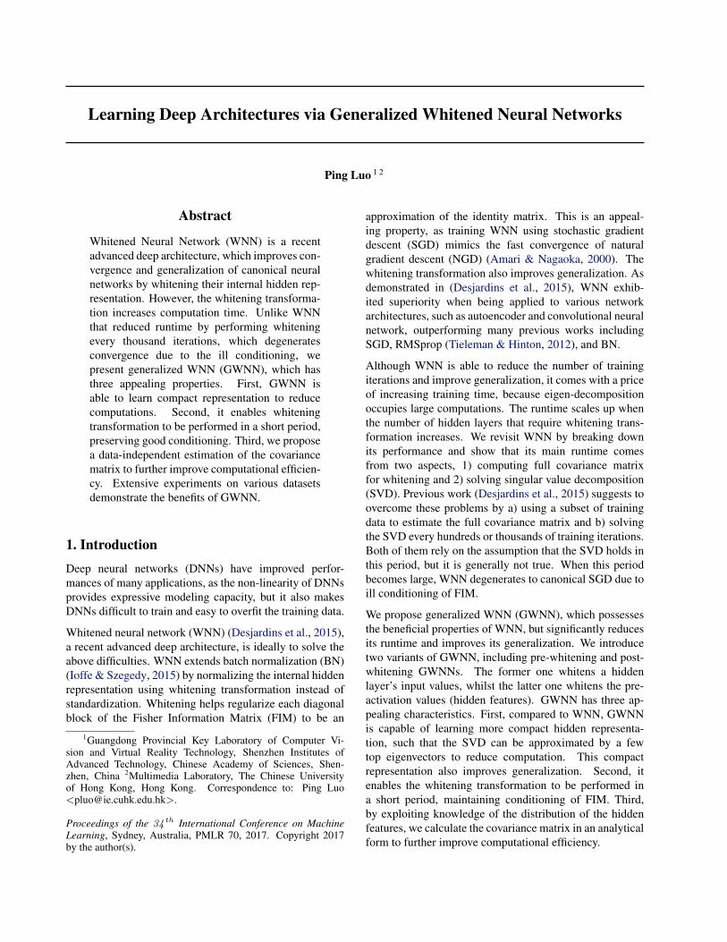
Figure 1. Comparisons of differnet architectures. An ordinary fully-connected (fc) layer can be adapted into (b) a whitened fc layer, (c)a pre-GWNN layer, and (d) a post-GWNN layer. (c) and (d) learn more compact representation than (b) does.

2. Notation and BackgroundWe begin by defining the basic notation for feed-forwardneural network. A neural network transforms an inputvector o0 to an output vector o` through a series of `hidden layers {oi}`i=1. We assume each layer has identicaldimension for the simplicity of notation i.e. ∀oi ∈ Rd×1.In this case, all vectors and matrixes in the followingshould have d rows unless otherwise stated. As shownin Fig.1 (a), each fully-connected (fc) layer consists ofa weight matrix, W i, and a set of hidden neurons, hi,each of which receives as input a weighted sum of outputsfrom the previous layer. We have hi = W ioi−1. Inthis work, we take fully-connected network as an example.Note that the above computation can be also applied to aconvolutional network, where an image patch is vectorizedas a column vector and represented by oi−1 and each rowof W i represents a filter.

As the recent deep architectures typically stack a batchnormalization (BN) layer before the pre-activation values,we do not explicitly include a bias term when computinghi, because it is normalized in BN, such that φi =hi−E[hi]√

Var[hi], where the expectation and variance are computed

over a minibatch of samples. LeCun et al. (2002) showedthat such normalization speeds up convergence even whenthe hidden features are not decorrelated. Furthermore,output of each layer is calculated by a nonlinear activationfunction. A popular choice is the rectified linear unit,relu(x) = max(0, x). The precise computation for anoutput is oi = max(0,diag(αi)φi + βi), where diag(x)represents a matrix whose diagonal entries are x. αi and βi

are two vectors that scale and shift the normalized features,in order to maintain the network’s representation capacity.

2.1. Whitened Neural Networks

This section revisits whitened neural networks (WNN).Any neural architecture can be adapted to a WNN bystacking a whitening transformation layer after the layer’sinput. For example, Fig.1 (b) adapts a fc layer as shown in

(a) into a whitened fc layer. Its information flow becomes

oi−1 = P i−1(oi−1 − µi−1), hi = W ioi−1, (1)

φi = hi√Var[hi]

, oi = max(0,diag(αi)φi + βi),

where µi−1 represents a centering variable, µi−1 =E[oi−1]. P i−1 is a whitening matrix whose rows areobtained from eigen-decomposition of Σi−1, which isthe covariance matrix of the input, Σi−1 = E[(oi−1 −µi−1)(oi−1 − µi−1)T]. The input is decorrelated by P i−1

in the sense that its covariance matrix becomes an identitymatrix, i.e. E[oi−1oi−1

T

] = I . To avoid ambiguity, we use‘ˆ’ to distinguish the variables in WNN and the canonicalfc layer whenever necessary. For instance, W i represents awhitened weight matrix. In Eqn.(1), computation of theBN layer has been simplified because we have E[hi] =W iP i−1(E[oi−1]− µi−1) = 0.

We define θ to be a vector consisting of all thewhitened weight matrixes concatenated together, θ ={vec(W 1)T, vec(W 2)T, ..., vec(W `)T}, where vec(·) is anoperator that vectorizes a matrix by stacking its columns.Let L(o`, y; θ) denote a loss function of WNN, whichmeasures the disagreement between a prediction o` madeby the network, and a target y. WNN is trained byminimizing the loss function with respect to the parametervector θ and two constraints

minθ

L(o`, y; θ) (2)

s.t. E[oi−1oi−1T

] = I, hi − E[hi] = hi, i = 1...`.

To satisfy the first constraint, P i−1 is obtained by decom-posing the covariance matrix, Σi−1 = U i−1Si−1U i−1

T.We choose P i−1 = (Si−1)−

12U i−1

T, where Si−1 is adiagonal matrix whose diagonal elements are eigenvaluesand U i−1 is an orthogonal matrix of eigenvectors. Thefirst constraint holds under the construction of eigen-decomposition.

The second constraint, hi − E[hi] = hi, enforces thatthe centered hidden features are the same, before and after

Generalized Whitened Neural Network

adapting a fc layer to WNN, as shown in Fig.1 (a) and (b).In other words, it ensures that their representation powersare identical. By combing the computations in Fig.1 (a) andEqn.(1), the second constraint implies that ‖(hi−E[hi])−hi‖22 = ‖(W ioi−1 − W iµi−1) − W ioi−1‖22 = 0, whichhas a closed-form solution, W i = W i(P i−1)−1. To seethis, we have hi = W i(P i−1)−1P i−1(oi−1 − µi−1) =W i(oi−1−µi−1) = hi−E[hi]. The representation capacitycan be preserved by mapping the whitened weight matrixfrom the ordinary weight matrix.

Conditioning of the FIM. Here we show that WNNimproves training efficiency by conditioning the Fisherinformation matrix (FIM) (Amari & Nagaoka, 2000). AFIM, denoted as F , consists of `× ` blocks. Each block isindexed by Fij , representing the covariance (co-adaptation)between the whitened weight matrixes of the i-th and j-thlayers. We have Fij = E[vec(δW i)vec(δW j)T], whereδW i indicates the gradient of the i-th whitened weightmatrix. For example, the gradient of W i is achieved byoi−1(δhi)T, as illustrated in Eqn.(1). We have vec(δW i) =

vec(oi−1(δhi)T) = δhi ⊗ oi−1, where ⊗ denotes theKronecker product. In this case, Fij can be rewrittenas E[(δhi ⊗ oi−1)(δhj ⊗ oj−1)T] = E[δhi(δhj)T ⊗oi−1(oj−1)T]. By assuming δh and o are independent asdemonstrated in (Raiko et al., 2012), Fij can be approx-imated by E[δhi(δhj)T] ⊗ E[oi−1(oj−1)T]. As a result,when i = j, each diagonal block of F , Fii, has a blockdiagonal structure because we have E[oi−1(oi−1)T] = I asshown in Eqn.(2), which improves conditioning of FIM andthus speeds up training. In general, WNN regularizes thediagonal blocks of FIM and achieves stronger conditioningthan those methods (LeCun et al., 2002; Tieleman &Hinton, 2012) that regularized the diagonal entries.

Training WNN. Alg.1 summarizes training of WNN. Atthe 1st line, the whitened weight matrix W i

0 is initializedby W i of the ordinary fc layer, which can be pretrainedor sampled from a Gaussian distribution. The 4th lineshows that W i

t is updated in each iteration t using SGD.The first and second constraints are achieved in the 7th and8th lines respectively. For example, the 8th line ensuresthat the hidden features are the same before and afterupdating the whitening matrix. As the distribution of thehidden representation changes after every update of thewhitened weight matrix, to maintain good conditioning ofFIM, the whitening matrix, P i−1, needs to be reconstructedfrequently by performing eigen-decomposition on Σi−1,which is estimated using N samples. N is typically104 in experiments. However, this raw strategy increasescomputation time. Desjardins et al. (2015) performedwhitening in every τ iterations as shown in the 5th line ofAlg.1 to reduce computations, e.g. τ = 103.

How good is the conditioning of the FIM by using Al-

Algorithm 1 Training WNN1: Init: initial network parameters θ, αi, βi; whitening matrixP i−1 = I; iteration t = 0; W i

t = W i; ∀i ∈ {1...`}.2: repeat3: for i = 1 to ` do4: update whitened weight matrix W i

t and parametersαit, β

it using SGD.

5: if mod(t, τ) = 0 then6: store old whitening matrix P i−1

o = P i−1.7: construct new matrix P i−1 by eigen-decomposition

on Σi−1, which is estimated using N samples.8: transform weight matrix W i

t = W itP

i−1o (P i−1)−1.

9: end if10: end for11: t = t+ 1.12: until convergence

0.5

0

1.0

(a) (b) (c) (d)

0.34

0.35 0.65 0.95

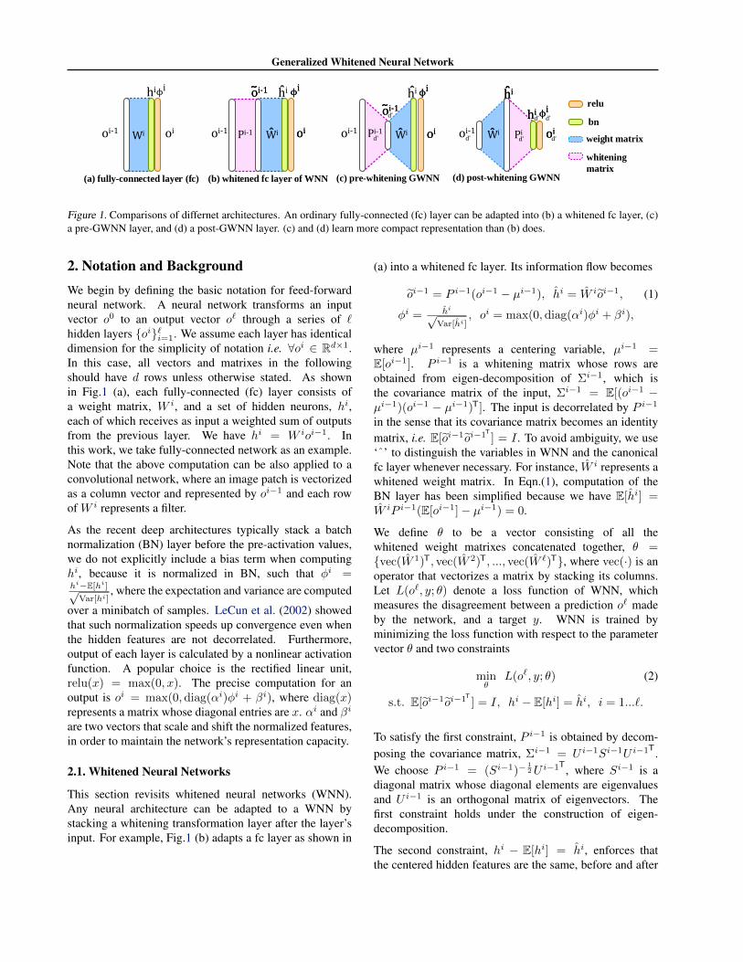
Figure 2. Visualizations of different covariance matrixes (a)-(d),which have different Pearson’s correlations (top) with respect toan identity matrix. Larger Pearson’s correlation indicates higherorthogonality. (a,b) are sampled from a uniform distributionbetween 0 and 1. (c,d) are generated by truncating a randomorthogonal matrix with different numbers of columns. Thecolorbar (right) indicates the value of each entry in these matrixes.

g.1? We measure the similarity of the covariance matrix,E[oi−1(oi−1)T], with the identity matrix I . This is calledthe orthogonality. We employ Pearson’s correlation1 as thesimilarity between two matrixes. Intuitively, this measurehas a value between −1 and +1, representing negativeand positive correlations. Larger values indicate higherorthogonality. Fig.2 visualizes four randomly generatedcovariance matrixes, where (a,b) are sampled from auniform distribution between 0 and 1. Fig.2 (c,d) aregenerated by truncating different numbers of columns of arandomly generated orthogonal matrix. For instance, (a,b)have small similarity with respect to the identity matrix.In contrast, when the correlation equals 0.65 as shown in(c), all entries in the diagonal are larger than 0.9 and morethan 80% off-diagonal entries have values smaller than 0.1.Furthermore, Pearson’s correlation is insensitive to the sizeof matrix, such that orthogonality of different layers canbe compared together. For example, although matrixes in

1Given an identity matrix, I , and a covariance matrix, Σ, thePearson’s correlation between them is defined as corr(Σ, I) =

vec(Σ)Tvec(I)√vec(Σ)Tvec(Σ)·vec(I)Tvec(I)

, where vec(Σ) is a normalized vec-

tor by subtracting mean of all entries.

Generalized Whitened Neural Network

0

0.1

0.2

0.3

0.4

0.5

0.6

0.7

0.8

0.9

1

1.1

0 1 2 3 4

orth

ogon

ality

iterations (1e3)

conv1conv4conv7

0

0.1

0.2

0.3

0.4

0.5

0.6

0.7

0.8

0.9

1

1.1

0 1 2 3 4

orth

ogon

ality

iterations (1e3)

conv1conv4conv7

5 5

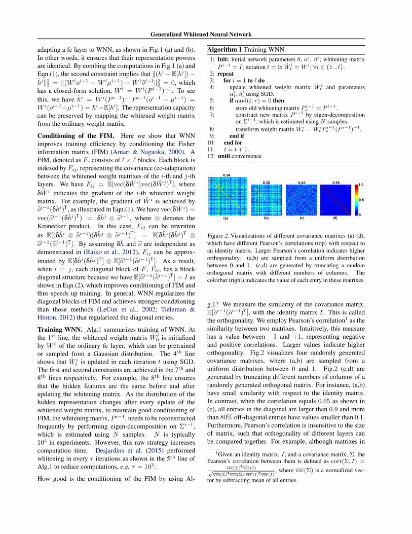
（a）WNN （b）pre-GWNN

Figure 3. Comparisons of conditioning when training a network-in-network (Lin et al., 2014) on CIFAR-10 (Krizhevsky, 2009)by using (a) WNN and (b) pre-GWNN. Compared to (b),the orthogonalities of three different layers in (a) have largefluctuations due to the ill conditioning of whitening, which isperformed in a large period τ . As a result, when τ increases,WNN will degenerate to the canonical SGD.

(a) and (b) have different sizes, they have similar valueof orthogonality when they are sampled from the samedistribution.

As shown in Fig.3 (a), we adopt network-in-network(NIN) (Lin et al., 2014) that is trained on CIFAR-10(Krizhevsky, 2009), and plot the orthogonalities of threedifferent convolutional layers, which are whitened everyτ = 103 iterations by using Alg.1. We see that or-thogonality values during training have large fluctuationsexcept those of the first convolutional layer, abbreviated as‘conv1’. This is because the distributions of deeper layers’inputs change after the whitened weight matrixes havebeen updated, leading to ill-conditions of the whiteningmatrixes, which are estimated in a large interval. In fact,large τ will degenerate WNN to canonical SGD. However,‘conv1’ uses image data as inputs, whose distribution istypically stable during training. Its whitening matrix canbe estimated once at the beginning and fixed in the entiretraining stage.

In the section below, we present generalized whitenedneural networks to improve conditioning of FIM whilereducing computation time.

3. Generalized Whitened Neural NetworksWe present two types of generalized WNN (GWNN), in-cluding pre-whitening and post-whitening GWNNs. Bothmodels share beneficial properties of WNN, but have lowercomputation time.

3.1. Pre-whitening GWNN

This section introduces pre-whitening GWNN, abbreviatedas pre-GWNN, which performs whitening transformationbefore applying the weight matrix (i.e. whiten the input),

as illustrated in Fig.1 (c). When adapting a fc layer topre-GWNN, the whitening matrix is truncated by removingthose eigenvectors that have small eigenvalues, in order tolearn compact representation. This allows the input vectorto vary its length, so as to gradually adapt the learnedrepresentation to informative patterns with high variations,but not noises. Learning pre-GWNN is formulated analo-gously to learning WNN in Eqn.(2), but with one additionalconstraint truncated the rank of the whitening matrix,

minθ

L(o`, y; θ) (3)

s.t. rank(P i−1) ≤ d′, E[oi−1d′ oi−1T

d′ ] = I,

hi − E[hi] = hi, i = 1...`.

Let d be the dimension of the original fc layer. By combin-ing Eqn.(2), we have P i−1 = (Si−1)−

12U i−1

T ∈ Rd×d,which is truncated by using P i−1d′ = (Si−1d′ )−

12U i−1d′

T ∈Rd′×d, where Si−1d′ is achieved by keeping rows andcolumns associated with the first d′ large eigenvalues,whilst U i−1d′ contains the corresponding d′ eigenvectors.The value of d′ can be tuned using a validation set.For simplicity, we choose d′ = d

2 , which works wellthroughout our experiments. This is inspired by the findingin (Zhang et al., 2015), who disclosed that the first 50%eigenvectors contribute over 95% energy in a deep model.

More specifically, pre-GWNN first projects an input vectorto a d′ low-dimensional space, oi−1d′ = P i−1d′ (oi−1 −µi−1) ∈ Rd′×1. The whitened weight matrix thenproduces a hidden feature vector of d dimensions, whichhas the same length as the ordinary fc layer, i.e. hi =W ioi−1d′ ∈ Rd×1, where W i = W i(P i−1d′ )−1 ∈ Rd×d′ .The computations of BN and the nonlinear activation areidentical to Eqn.(1).

Training pre-GWNN is similar to Alg.1. The mainmodification is produced at the 7th line in order to reduceruntime. Although Alg.1 decreases number of iterationswhen training converged, each iteration has additionalcomputation time for eigen-decomposition. For example,in WNN, the required computation of full singular valuedecomposition (SVD) is typically O(Nd2), where Nrepresents the number of samples employed to estimatethe covariance matrix. In particular, when we have `whitened layers and T is the number of iterations, allwhitening transformations occupy O(Nd

2T`τ ) runtime in

the entire training stage. In contrast, pre-GWNN performsthe popular online estimation for the top d′ eigenvectorsin P i−1d′ such as online SVD (Shamir, 2015; Povey et al.,2015), instead of using full SVD as WNN did. Thisdifference reduces runtime to O( (N+M)d′T`

τ ′ ), where τ ′

represents the whitening interval in GWNN and M is thenumber of samples used to estimate the top eigenvectors.We have M = N as employed in previous works.

Generalized Whitened Neural Network

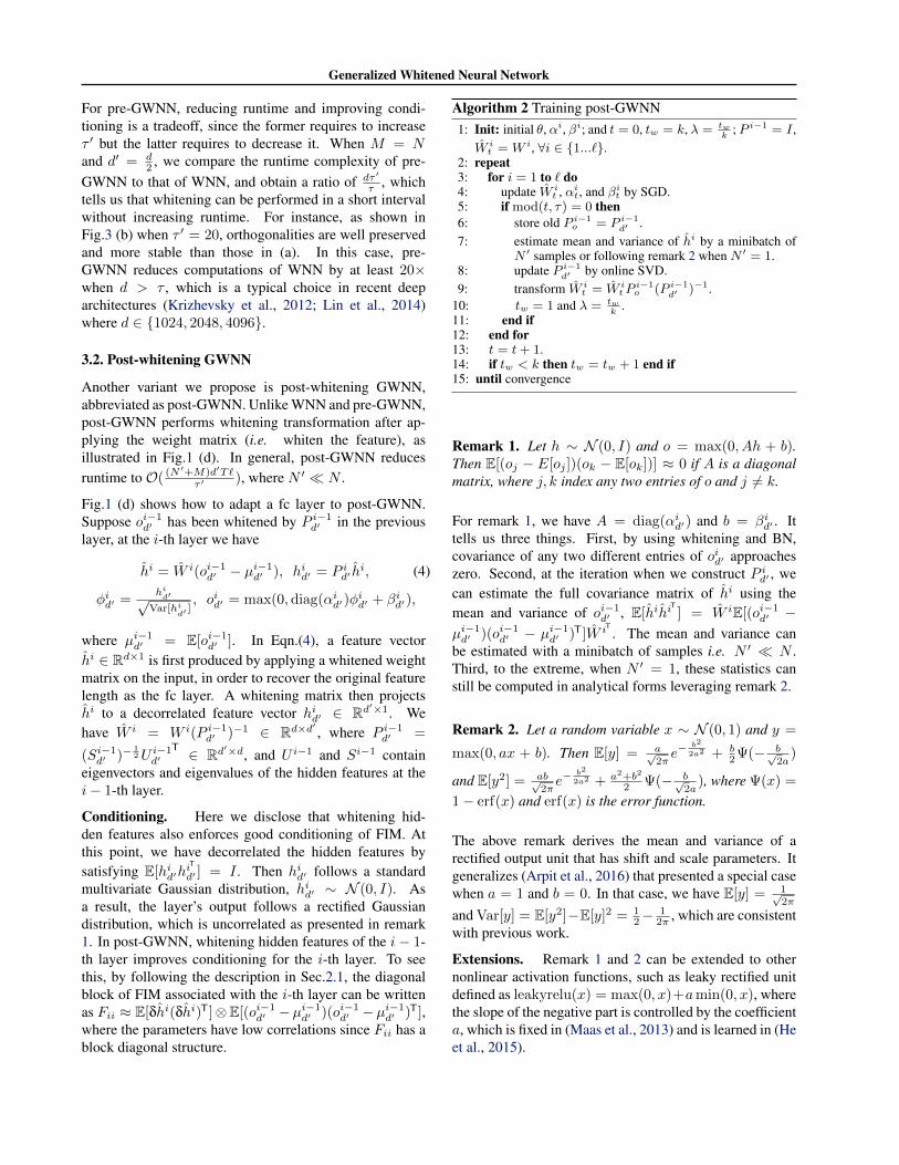
For pre-GWNN, reducing runtime and improving condi-tioning is a tradeoff, since the former requires to increaseτ ′ but the latter requires to decrease it. When M = Nand d′ = d

2 , we compare the runtime complexity of pre-GWNN to that of WNN, and obtain a ratio of dτ ′

τ , whichtells us that whitening can be performed in a short intervalwithout increasing runtime. For instance, as shown inFig.3 (b) when τ ′ = 20, orthogonalities are well preservedand more stable than those in (a). In this case, pre-GWNN reduces computations of WNN by at least 20×when d > τ , which is a typical choice in recent deeparchitectures (Krizhevsky et al., 2012; Lin et al., 2014)where d ∈ {1024, 2048, 4096}.

3.2. Post-whitening GWNN

Another variant we propose is post-whitening GWNN,abbreviated as post-GWNN. Unlike WNN and pre-GWNN,post-GWNN performs whitening transformation after ap-plying the weight matrix (i.e. whiten the feature), asillustrated in Fig.1 (d). In general, post-GWNN reducesruntime to O( (N ′+M)d′T`

τ ′ ), where N ′ � N .

Fig.1 (d) shows how to adapt a fc layer to post-GWNN.Suppose oi−1d′ has been whitened by P i−1d′ in the previouslayer, at the i-th layer we have

hi = W i(oi−1d′ − µi−1d′ ), hid′ = P id′ h

i, (4)

φid′ =hid′√

Var[hid′ ], oid′ = max(0,diag(αid′)φ

id′ + βid′),

where µi−1d′ = E[oi−1d′ ]. In Eqn.(4), a feature vectorhi ∈ Rd×1 is first produced by applying a whitened weightmatrix on the input, in order to recover the original featurelength as the fc layer. A whitening matrix then projectshi to a decorrelated feature vector hid′ ∈ Rd′×1. Wehave W i = W i(P i−1d′ )−1 ∈ Rd×d′ , where P i−1d′ =

(Si−1d′ )−12U i−1d′

T ∈ Rd′×d, and U i−1 and Si−1 containeigenvectors and eigenvalues of the hidden features at thei− 1-th layer.

Conditioning. Here we disclose that whitening hid-den features also enforces good conditioning of FIM. Atthis point, we have decorrelated the hidden features bysatisfying E[hid′h

iT

d′ ] = I . Then hid′ follows a standardmultivariate Gaussian distribution, hid′ ∼ N (0, I). Asa result, the layer’s output follows a rectified Gaussiandistribution, which is uncorrelated as presented in remark1. In post-GWNN, whitening hidden features of the i− 1-th layer improves conditioning for the i-th layer. To seethis, by following the description in Sec.2.1, the diagonalblock of FIM associated with the i-th layer can be writtenas Fii ≈ E[δhi(δhi)T]⊗E[(oi−1d′ −µ

i−1d′ )(oi−1d′ −µ

i−1d′ )T],

where the parameters have low correlations since Fii has ablock diagonal structure.

Algorithm 2 Training post-GWNN1: Init: initial θ, αi, βi; and t = 0, tw = k, λ = tw

k; P i−1 = I ,

W it = W i, ∀i ∈ {1...`}.

2: repeat3: for i = 1 to ` do4: update W i

t , αit, and βi

t by SGD.5: if mod(t, τ) = 0 then6: store old P i−1

o = P i−1d′ .

7: estimate mean and variance of hi by a minibatch ofN ′ samples or following remark 2 when N ′ = 1.

8: update P i−1d′ by online SVD.

9: transform W it = W i

tPi−1o (P i−1

d′ )−1.10: tw = 1 and λ = tw

k.

11: end if12: end for13: t = t+ 1.14: if tw < k then tw = tw + 1 end if15: until convergence

Remark 1. Let h ∼ N (0, I) and o = max(0, Ah + b).Then E[(oj − E[oj ])(ok − E[ok])] ≈ 0 if A is a diagonalmatrix, where j, k index any two entries of o and j 6= k.

For remark 1, we have A = diag(αid′) and b = βid′ . Ittells us three things. First, by using whitening and BN,covariance of any two different entries of oid′ approacheszero. Second, at the iteration when we construct P id′ , wecan estimate the full covariance matrix of hi using themean and variance of oi−1d′ , E[hihi

T

] = W iE[(oi−1d′ −µi−1d′ )(oi−1d′ − µi−1d′ )T]W iT . The mean and variance canbe estimated with a minibatch of samples i.e. N ′ � N .Third, to the extreme, when N ′ = 1, these statistics canstill be computed in analytical forms leveraging remark 2.

Remark 2. Let a random variable x ∼ N (0, 1) and y =

max(0, ax + b). Then E[y] = a√2πe−

b2

2a2 + b2Ψ(− b√

2a)

and E[y2] = ab√2πe−

b2

2a2 + a2+b2

2 Ψ(− b√2a

), where Ψ(x) =

1− erf(x) and erf(x) is the error function.

The above remark derives the mean and variance of arectified output unit that has shift and scale parameters. Itgeneralizes (Arpit et al., 2016) that presented a special casewhen a = 1 and b = 0. In that case, we have E[y] = 1√

2π

and Var[y] = E[y2]−E[y]2 = 12−

12π , which are consistent

with previous work.

Extensions. Remark 1 and 2 can be extended to othernonlinear activation functions, such as leaky rectified unitdefined as leakyrelu(x) = max(0, x)+amin(0, x), wherethe slope of the negative part is controlled by the coefficienta, which is fixed in (Maas et al., 2013) and is learned in (Heet al., 2015).

Generalized Whitened Neural Network

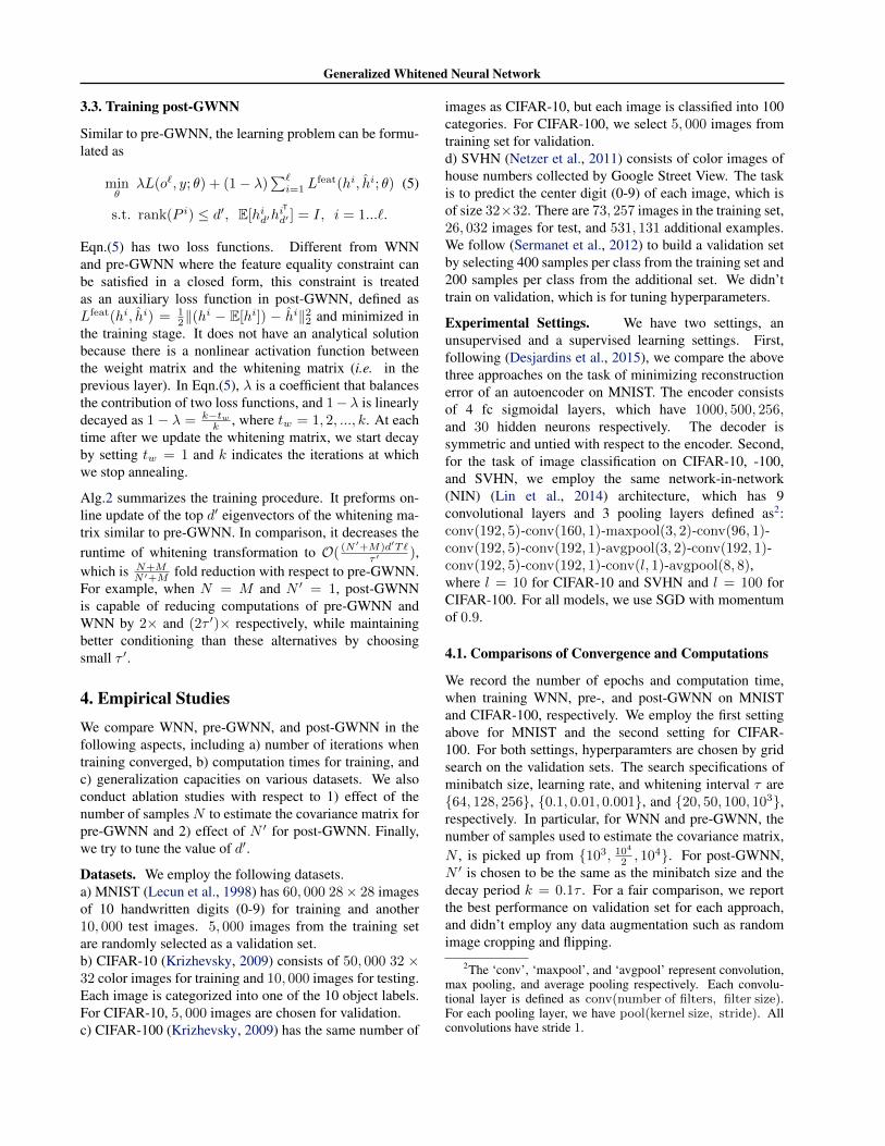
3.3. Training post-GWNN

Similar to pre-GWNN, the learning problem can be formu-lated as

minθ

λL(o`, y; θ) + (1− λ)∑`i=1 L

feat(hi, hi; θ) (5)

s.t. rank(P i) ≤ d′, E[hid′hiT

d′ ] = I, i = 1...`.

Eqn.(5) has two loss functions. Different from WNNand pre-GWNN where the feature equality constraint canbe satisfied in a closed form, this constraint is treatedas an auxiliary loss function in post-GWNN, defined asLfeat(hi, hi) = 1

2‖(hi − E[hi]) − hi‖22 and minimized in

the training stage. It does not have an analytical solutionbecause there is a nonlinear activation function betweenthe weight matrix and the whitening matrix (i.e. in theprevious layer). In Eqn.(5), λ is a coefficient that balancesthe contribution of two loss functions, and 1− λ is linearlydecayed as 1− λ = k−tw

k , where tw = 1, 2, ..., k. At eachtime after we update the whitening matrix, we start decayby setting tw = 1 and k indicates the iterations at whichwe stop annealing.

Alg.2 summarizes the training procedure. It preforms on-line update of the top d′ eigenvectors of the whitening ma-trix similar to pre-GWNN. In comparison, it decreases theruntime of whitening transformation to O( (N ′+M)d′T`

τ ′ ),which is N+M

N ′+M fold reduction with respect to pre-GWNN.For example, when N = M and N ′ = 1, post-GWNNis capable of reducing computations of pre-GWNN andWNN by 2× and (2τ ′)× respectively, while maintainingbetter conditioning than these alternatives by choosingsmall τ ′.

4. Empirical StudiesWe compare WNN, pre-GWNN, and post-GWNN in thefollowing aspects, including a) number of iterations whentraining converged, b) computation times for training, andc) generalization capacities on various datasets. We alsoconduct ablation studies with respect to 1) effect of thenumber of samples N to estimate the covariance matrix forpre-GWNN and 2) effect of N ′ for post-GWNN. Finally,we try to tune the value of d′.

Datasets. We employ the following datasets.a) MNIST (Lecun et al., 1998) has 60, 000 28× 28 imagesof 10 handwritten digits (0-9) for training and another10, 000 test images. 5, 000 images from the training setare randomly selected as a validation set.b) CIFAR-10 (Krizhevsky, 2009) consists of 50, 000 32 ×32 color images for training and 10, 000 images for testing.Each image is categorized into one of the 10 object labels.For CIFAR-10, 5, 000 images are chosen for validation.c) CIFAR-100 (Krizhevsky, 2009) has the same number of

images as CIFAR-10, but each image is classified into 100categories. For CIFAR-100, we select 5, 000 images fromtraining set for validation.d) SVHN (Netzer et al., 2011) consists of color images ofhouse numbers collected by Google Street View. The taskis to predict the center digit (0-9) of each image, which isof size 32×32. There are 73, 257 images in the training set,26, 032 images for test, and 531, 131 additional examples.We follow (Sermanet et al., 2012) to build a validation setby selecting 400 samples per class from the training set and200 samples per class from the additional set. We didn’ttrain on validation, which is for tuning hyperparameters.

Experimental Settings. We have two settings, anunsupervised and a supervised learning settings. First,following (Desjardins et al., 2015), we compare the abovethree approaches on the task of minimizing reconstructionerror of an autoencoder on MNIST. The encoder consistsof 4 fc sigmoidal layers, which have 1000, 500, 256,and 30 hidden neurons respectively. The decoder issymmetric and untied with respect to the encoder. Second,for the task of image classification on CIFAR-10, -100,and SVHN, we employ the same network-in-network(NIN) (Lin et al., 2014) architecture, which has 9convolutional layers and 3 pooling layers defined as2:conv(192, 5)-conv(160, 1)-maxpool(3, 2)-conv(96, 1)-conv(192, 5)-conv(192, 1)-avgpool(3, 2)-conv(192, 1)-conv(192, 5)-conv(192, 1)-conv(l, 1)-avgpool(8, 8),where l = 10 for CIFAR-10 and SVHN and l = 100 forCIFAR-100. For all models, we use SGD with momentumof 0.9.

4.1. Comparisons of Convergence and Computations

We record the number of epochs and computation time,when training WNN, pre-, and post-GWNN on MNISTand CIFAR-100, respectively. We employ the first settingabove for MNIST and the second setting for CIFAR-100. For both settings, hyperparamters are chosen by gridsearch on the validation sets. The search specifications ofminibatch size, learning rate, and whitening interval τ are{64, 128, 256}, {0.1, 0.01, 0.001}, and {20, 50, 100, 103},respectively. In particular, for WNN and pre-GWNN, thenumber of samples used to estimate the covariance matrix,N , is picked up from {103, 10

4

2 , 104}. For post-GWNN,N ′ is chosen to be the same as the minibatch size and thedecay period k = 0.1τ . For a fair comparison, we reportthe best performance on validation set for each approach,and didn’t employ any data augmentation such as randomimage cropping and flipping.

2The ‘conv’, ‘maxpool’, and ‘avgpool’ represent convolution,max pooling, and average pooling respectively. Each convolu-tional layer is defined as conv(number of filters, filter size).For each pooling layer, we have pool(kernel size, stride). Allconvolutions have stride 1.

Generalized Whitened Neural Network

0

0.1

0.2

0.3

0.4

0.5

0.6

0.7

0.8

0 5 10 15 20 25 30 35

testerror

minutes

SGDpost‐GWNNpre‐GWNNWNN

0

0.1

0.2

0.3

0.4

0.5

0.6

0.7

0.8

0 2 4 6 8 10 12 14 16 18

validationerror

epochs

SGDpost‐GWNNpre‐GWNNWNN

0.4

0.5

0.6

0.7

0.8

0.9

1

0 0.2 0.4 0.6 0.8 1 1.2 1.4

testerror

hour

SGDpost‐GWNNpre‐GWNNWNN

0.4

0.5

0.6

0.7

0.8

0.9

1

0 3 6 9 12 15 18 21 24

validationerror

epochs

SGDpost‐GWNNpre‐GWNNWNN

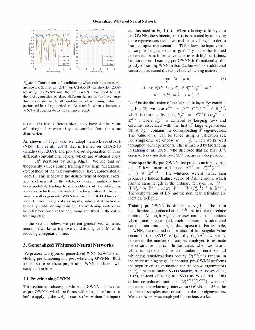
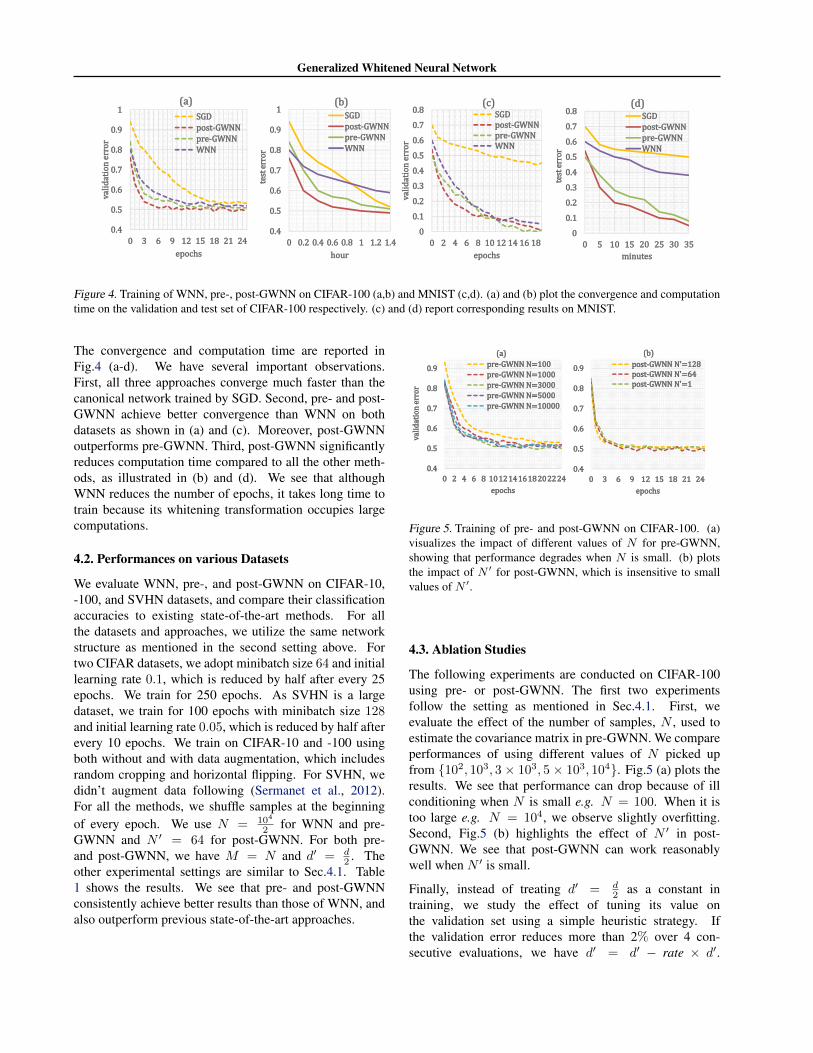
(a) (b) (c) (d)

Figure 4. Training of WNN, pre-, post-GWNN on CIFAR-100 (a,b) and MNIST (c,d). (a) and (b) plot the convergence and computationtime on the validation and test set of CIFAR-100 respectively. (c) and (d) report corresponding results on MNIST.

The convergence and computation time are reported inFig.4 (a-d). We have several important observations.First, all three approaches converge much faster than thecanonical network trained by SGD. Second, pre- and post-GWNN achieve better convergence than WNN on bothdatasets as shown in (a) and (c). Moreover, post-GWNNoutperforms pre-GWNN. Third, post-GWNN significantlyreduces computation time compared to all the other meth-ods, as illustrated in (b) and (d). We see that althoughWNN reduces the number of epochs, it takes long time totrain because its whitening transformation occupies largecomputations.

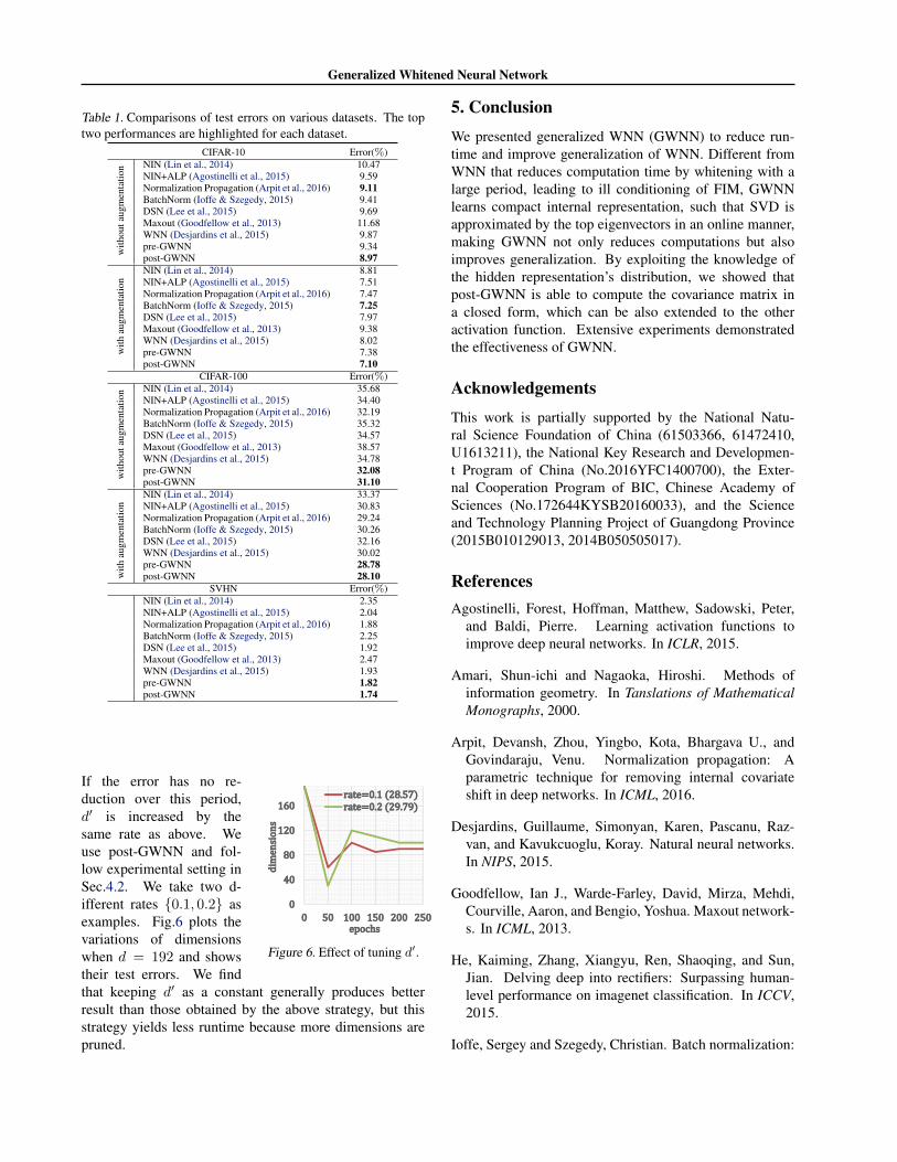
4.2. Performances on various Datasets

We evaluate WNN, pre-, and post-GWNN on CIFAR-10,-100, and SVHN datasets, and compare their classificationaccuracies to existing state-of-the-art methods. For allthe datasets and approaches, we utilize the same networkstructure as mentioned in the second setting above. Fortwo CIFAR datasets, we adopt minibatch size 64 and initiallearning rate 0.1, which is reduced by half after every 25epochs. We train for 250 epochs. As SVHN is a largedataset, we train for 100 epochs with minibatch size 128and initial learning rate 0.05, which is reduced by half afterevery 10 epochs. We train on CIFAR-10 and -100 usingboth without and with data augmentation, which includesrandom cropping and horizontal flipping. For SVHN, wedidn’t augment data following (Sermanet et al., 2012).For all the methods, we shuffle samples at the beginningof every epoch. We use N = 104

2 for WNN and pre-GWNN and N ′ = 64 for post-GWNN. For both pre-and post-GWNN, we have M = N and d′ = d

2 . Theother experimental settings are similar to Sec.4.1. Table1 shows the results. We see that pre- and post-GWNNconsistently achieve better results than those of WNN, andalso outperform previous state-of-the-art approaches.

0.4

0.5

0.6

0.7

0.8

0.9

0 3 6 9 12 15 18 21 24epochs

post‐GWNNN' 128post‐GWNNN' 64post‐GWNNN' 1

0.4

0.5

0.6

0.7

0.8

0.9

0 2 4 6 8 1012141618202224

validationerror

epochs

pre‐GWNNN 100pre‐GWNNN 1000pre‐GWNNN 3000pre‐GWNNN 5000pre‐GWNNN 10000

(a) (b)

Figure 5. Training of pre- and post-GWNN on CIFAR-100. (a)visualizes the impact of different values of N for pre-GWNN,showing that performance degrades when N is small. (b) plotsthe impact of N ′ for post-GWNN, which is insensitive to smallvalues of N ′.

4.3. Ablation Studies

The following experiments are conducted on CIFAR-100using pre- or post-GWNN. The first two experimentsfollow the setting as mentioned in Sec.4.1. First, weevaluate the effect of the number of samples, N , used toestimate the covariance matrix in pre-GWNN. We compareperformances of using different values of N picked upfrom {102, 103, 3 × 103, 5 × 103, 104}. Fig.5 (a) plots theresults. We see that performance can drop because of illconditioning when N is small e.g. N = 100. When it istoo large e.g. N = 104, we observe slightly overfitting.Second, Fig.5 (b) highlights the effect of N ′ in post-GWNN. We see that post-GWNN can work reasonablywell when N ′ is small.

Finally, instead of treating d′ = d2 as a constant in

training, we study the effect of tuning its value onthe validation set using a simple heuristic strategy. Ifthe validation error reduces more than 2% over 4 con-secutive evaluations, we have d′ = d′ − rate × d′.

Generalized Whitened Neural Network

Table 1. Comparisons of test errors on various datasets. The toptwo performances are highlighted for each dataset.

CIFAR-10 Error(%)

with

outa

ugm

enta

tion NIN (Lin et al., 2014) 10.47

NIN+ALP (Agostinelli et al., 2015) 9.59Normalization Propagation (Arpit et al., 2016) 9.11BatchNorm (Ioffe & Szegedy, 2015) 9.41DSN (Lee et al., 2015) 9.69Maxout (Goodfellow et al., 2013) 11.68WNN (Desjardins et al., 2015) 9.87pre-GWNN 9.34post-GWNN 8.97

with

augm

enta

tion

NIN (Lin et al., 2014) 8.81NIN+ALP (Agostinelli et al., 2015) 7.51Normalization Propagation (Arpit et al., 2016) 7.47BatchNorm (Ioffe & Szegedy, 2015) 7.25DSN (Lee et al., 2015) 7.97Maxout (Goodfellow et al., 2013) 9.38WNN (Desjardins et al., 2015) 8.02pre-GWNN 7.38post-GWNN 7.10

CIFAR-100 Error(%)

with

outa

ugm

enta

tion NIN (Lin et al., 2014) 35.68

NIN+ALP (Agostinelli et al., 2015) 34.40Normalization Propagation (Arpit et al., 2016) 32.19BatchNorm (Ioffe & Szegedy, 2015) 35.32DSN (Lee et al., 2015) 34.57Maxout (Goodfellow et al., 2013) 38.57WNN (Desjardins et al., 2015) 34.78pre-GWNN 32.08post-GWNN 31.10

with

augm

enta

tion

NIN (Lin et al., 2014) 33.37NIN+ALP (Agostinelli et al., 2015) 30.83Normalization Propagation (Arpit et al., 2016) 29.24BatchNorm (Ioffe & Szegedy, 2015) 30.26DSN (Lee et al., 2015) 32.16WNN (Desjardins et al., 2015) 30.02pre-GWNN 28.78post-GWNN 28.10

SVHN Error(%)NIN (Lin et al., 2014) 2.35NIN+ALP (Agostinelli et al., 2015) 2.04Normalization Propagation (Arpit et al., 2016) 1.88BatchNorm (Ioffe & Szegedy, 2015) 2.25DSN (Lee et al., 2015) 1.92Maxout (Goodfellow et al., 2013) 2.47WNN (Desjardins et al., 2015) 1.93pre-GWNN 1.82post-GWNN 1.74

0

40

80

120

160

0 50 100 150 200 250

dimensions

epochs

rate 0.1 28.57rate 0.2 29.79

Figure 6. Effect of tuning d′.

If the error has no re-duction over this period,d′ is increased by thesame rate as above. Weuse post-GWNN and fol-low experimental setting inSec.4.2. We take two d-ifferent rates {0.1, 0.2} asexamples. Fig.6 plots thevariations of dimensionswhen d = 192 and showstheir test errors. We findthat keeping d′ as a constant generally produces betterresult than those obtained by the above strategy, but thisstrategy yields less runtime because more dimensions arepruned.

5. ConclusionWe presented generalized WNN (GWNN) to reduce run-time and improve generalization of WNN. Different fromWNN that reduces computation time by whitening with alarge period, leading to ill conditioning of FIM, GWNNlearns compact internal representation, such that SVD isapproximated by the top eigenvectors in an online manner,making GWNN not only reduces computations but alsoimproves generalization. By exploiting the knowledge ofthe hidden representation’s distribution, we showed thatpost-GWNN is able to compute the covariance matrix ina closed form, which can be also extended to the otheractivation function. Extensive experiments demonstratedthe effectiveness of GWNN.

AcknowledgementsThis work is partially supported by the National Natu-ral Science Foundation of China (61503366, 61472410,U1613211), the National Key Research and Developmen-t Program of China (No.2016YFC1400700), the Exter-nal Cooperation Program of BIC, Chinese Academy ofSciences (No.172644KYSB20160033), and the Scienceand Technology Planning Project of Guangdong Province(2015B010129013, 2014B050505017).

ReferencesAgostinelli, Forest, Hoffman, Matthew, Sadowski, Peter,

and Baldi, Pierre. Learning activation functions toimprove deep neural networks. In ICLR, 2015.

Amari, Shun-ichi and Nagaoka, Hiroshi. Methods ofinformation geometry. In Tanslations of MathematicalMonographs, 2000.

Arpit, Devansh, Zhou, Yingbo, Kota, Bhargava U., andGovindaraju, Venu. Normalization propagation: Aparametric technique for removing internal covariateshift in deep networks. In ICML, 2016.

Desjardins, Guillaume, Simonyan, Karen, Pascanu, Raz-van, and Kavukcuoglu, Koray. Natural neural networks.In NIPS, 2015.

Goodfellow, Ian J., Warde-Farley, David, Mirza, Mehdi,Courville, Aaron, and Bengio, Yoshua. Maxout network-s. In ICML, 2013.

He, Kaiming, Zhang, Xiangyu, Ren, Shaoqing, and Sun,Jian. Delving deep into rectifiers: Surpassing human-level performance on imagenet classification. In ICCV,2015.

Ioffe, Sergey and Szegedy, Christian. Batch normalization:

Generalized Whitened Neural Network

Accelerating deep network training by reducing internalcovariate shift. In ICML, 2015.

Krizhevsky, Alex. Learning multiple layers of featuresfrom tiny images. In Technical Report, 2009.

Krizhevsky, Alex, Sutskever, Ilya, and Hinton, Geoffrey E.Imagenet classification with deep convolutional neuralnetworks. In NIPS, 2012.

Lecun, Y., Bottou, L., Bengio, Y., and Haffner, P. Gradient-based learning applied to document recognition. InProceeding of IEEE, 1998.

LeCun, Yann, Bottou, Leon, Orr, Genevieve B., and Mller,Klaus Robert. Efficient backprop. In Neural Networks:Tricks of the Trade, 2002.

Lee, Chen-Yu, Xie, Saining, Gallagher, Patrick, Zhang,Zhengyou, and Tu, Zhuowen. Deeply-supervised nets.In AISTATS, 2015.

Lin, Min, Chen, Qiang, and Yan, Shuicheng. Network innetwork. In ICLR, 2014.

Maas, Andrew L., Hannun, Awni Y., , and Ng, Andrew Y.Rectifier nonlinearities improve neural network acousticmodels. In ICML, 2013.

Netzer, Y., Wang, T., Coates, A., Bissacco, A., Wu, B.,and Ng, A. Y. Reading digits in natural images withunsupervised feature learning. In NIPS Workshop onDeep Learning and Unsupervised Feature Learning,2011.

Povey, Daniel, Zhang, Xiaohui, and Khudanpur, Sanjeev.Parallel training of dnns with natural gradient and pa-rameter averaging. In ICLR workshop, 2015.

Raiko, Tapani, Valpola, Harri, and LeCun, Yann. Deeplearning made easier by linear transformations in per-ceptrons. In AISTATS, 2012.

Sermanet, Pierre, Chintala, Soumith, and LeCun, Yann.Convolutional neural networks applied to house numbersdigit classification. In arXiv:1204.3968, 2012.

Shamir, Ohad. A stochastic pca and svd algorithm with anexponential convergence rate. In ICML, 2015.

Tieleman, Tijmen and Hinton, Geoffrey. Rmsprop: Dividethe gradient by a running average of its recent magni-tude. In Neural Networks for Machine Learning (Lecture6.5), 2012.

Zhang, Xiangyu, Zou, Jianhua, He, Kaiming, and Sun,Jian. Accelerating very deep convolutional networks forclassification and detection. In IEEE Transactions onPattern Analysis and Machine Intelligence, 2015.