learning deep embeddings with histogram loss (nips2016)
TRANSCRIPT


l
l
l
l

Figure 4: (Left) Eight ILSVRC-2010 test images and the five labels considered most probable by our model.The correct label is written under each image, and the probability assigned to the correct label is also shownwith a red bar (if it happens to be in the top 5). (Right) Five ILSVRC-2010 test images in the first column. Theremaining columns show the six training images that produce feature vectors in the last hidden layer with thesmallest Euclidean distance from the feature vector for the test image.
In the left panel of Figure 4 we qualitatively assess what the network has learned by computing itstop-5 predictions on eight test images. Notice that even off-center objects, such as the mite in thetop-left, can be recognized by the net. Most of the top-5 labels appear reasonable. For example,only other types of cat are considered plausible labels for the leopard. In some cases (grille, cherry)there is genuine ambiguity about the intended focus of the photograph.
Another way to probe the network’s visual knowledge is to consider the feature activations inducedby an image at the last, 4096-dimensional hidden layer. If two images produce feature activationvectors with a small Euclidean separation, we can say that the higher levels of the neural networkconsider them to be similar. Figure 4 shows five images from the test set and the six images fromthe training set that are most similar to each of them according to this measure. Notice that at thepixel level, the retrieved training images are generally not close in L2 to the query images in the firstcolumn. For example, the retrieved dogs and elephants appear in a variety of poses. We present theresults for many more test images in the supplementary material.
Computing similarity by using Euclidean distance between two 4096-dimensional, real-valued vec-tors is inefficient, but it could be made efficient by training an auto-encoder to compress these vectorsto short binary codes. This should produce a much better image retrieval method than applying auto-encoders to the raw pixels [14], which does not make use of image labels and hence has a tendencyto retrieve images with similar patterns of edges, whether or not they are semantically similar.
7 Discussion
Our results show that a large, deep convolutional neural network is capable of achieving record-breaking results on a highly challenging dataset using purely supervised learning. It is notablethat our network’s performance degrades if a single convolutional layer is removed. For example,removing any of the middle layers results in a loss of about 2% for the top-1 performance of thenetwork. So the depth really is important for achieving our results.
To simplify our experiments, we did not use any unsupervised pre-training even though we expectthat it will help, especially if we obtain enough computational power to significantly increase thesize of the network without obtaining a corresponding increase in the amount of labeled data. Thusfar, our results have improved as we have made our network larger and trained it longer but we stillhave many orders of magnitude to go in order to match the infero-temporal pathway of the humanvisual system. Ultimately we would like to use very large and deep convolutional nets on videosequences where the temporal structure provides very helpful information that is missing or far lessobvious in static images.
8

l l

l
l l

l
l l

l
l l
l l

+
- input batch embedded batch similarity histograms
deep net aggregation
Figure 1: The histogram loss computation for a batch of examples (color-coded; same color indicates matchingsamples). After the batch (left) is embedded into a high-dimensional space by a deep network (middle), wecompute the histograms of similarities of positive (top-right) and negative pairs (bottom-right). We then evaluatethe integral of the product between the negative distribution and the cumulative density function for the positivedistribution (shown with a dashed line), which corresponds to a probability that a randomly sampled positivepair has smaller similarity than a randomly sampled negative pair. Such histogram loss can be minimized bybackpropagation. The only associated parameter of such loss is the number of histogram bins, to which theresults have very low sensitivity.
(as histograms with linearly-interpolated values-to-bins assignments). In the second stage, theoverlap between the two distributions is computed by estimating the probability that the two pointssampled from the two distribution are in a wrong order, i.e. that a random negative pair has a highersimilarity than a random positive pair. The two stages are implemented in a piecewise-differentiablemanner, thus allowing to minimize the loss (i.e. the overlap between distributions) using standardbackpropagation.
The number of bins in the histograms is the only tunable parameter associated with our loss, and itcan be set according to the batch size independently of the data itself. In the experiments, we fixthis parameter (and the batch size) and demonstrate the versatility of the loss by applying it to fourdifferent image datasets of varying complexity and nature. Comparing the new loss to state-of-the-artreveals its favourable performance. Overall, we hope that the proposed loss will be used as an“out-of-the-box” solution for learning deep embeddings that requires little tuning and leads to close tothe state-of-the-art results.
2 Related work
Recent works on learning embeddings use deep architectures (typically ConvNets [10; 8]) andstochastic optimization. Below we review the loss functions that have been used in recent works.
Classification losses. It has been observed in [8] and confirmed later in multiple works (e.g. [15])that deep networks trained for classification can be used for deep embedding. In particular, it issufficient to consider an intermediate representation arising in one of the last layers of the deepnetwork. The normalization is added post-hoc. Many of the works mentioned below pre-train theirembeddings as a part of the classification networks.
Pairwise losses. Methods that use pairwise losses sample pairs of training points and score themindependently. The pioneering work on deep embeddings [3] penalizes the deviation from the unitcosine similarity for positive pairs and the deviation from �1 or �0.9 for negative pairs. Perhaps,the most popular of pairwise losses is the contrastive loss [5; 20], which minimizes the distances inthe positive pairs and tries to maximize the distances in the negative pairs as long as these distancesare smaller than some margin M . Several works pointed to the fact that attempting to collapse allpositive pairs may lead to excessive overfitting and therefore suggested losses that mitigate thiseffect, e.g. a double-margin contrastive loss [12], which drops to zero for positive pairs as long astheir distances fall beyond the second (smaller) margin. Finally, several works use non-hinge basedpairwise losses such as log-sum-exp and cross-entropy on the similarity values that softly encouragethe similarity to be high for positive values and low for negative values (e.g. [27; 24]). The mainproblem with pairwise losses is that the margin parameters might be hard to tune, especially sincethe distributions of distances or similarities can be changing dramatically as the learning progresses.While most works “skip” the burn-in period by initializing the embedding to a network pre-trained
2


l
l
l
l

l l l
l l l
10
15
20
25
Embedding size
F1 s
core
(%
)
64 128 256 512
1024
GoogLeNet pool5
Contrastive
Triplet
LiftedStruct
83
84
85
86
87
88
Embedding size
NM
I sc
ore
(%
)
64 128 256 512
1024
GoogLeNet pool5
Contrastive
Triplet
LiftedStruct
1 10 100 1000
50
60
70
80
90
100
K
Rec
all@
K s
core
(%
)
GoogLeNet pool5
Contrastive
Triplet
LiftedStruct
Figure 9: F1, NMI, and Recall@K score metrics on the test split of Stanford Online Products with GoogLeNet [33].
Figure 10: Examples of successful queries on our StanfordOnline Products dataset using our embedding (size 512).Images in the first column are query images and the rest arefive nearest neighbors.
show some example queries and nearest neighbors on thedataset for both successful and failure cases. Despite thehuge changes in the viewpoint, configuration, and illumi-nation, our method can successfully retrieve examples fromthe same class and most retrieval failures come from finegrained subtle differences among similar products. Pleaserefer to the supplementary material for the t-SNE visual-
Figure 11: Examples of failure queries on Stanford OnlineProducts dataset. Most failures are fine grained subtle dif-ferences among similar products. Images in the first columnare query images and the rest are five nearest neighbors.
ization of the learned embedding on our Stanford OnlineProducts dataset.
8. ConclusionWe described a deep feature embedding and metric
learning algorithm which defines a novel structured predic-tion objective on the lifted pairwise distance matrix withinthe batch during the neural network training. The experi-mental results on CUB-200-2011 [37], CARS196 [19], andStanford Online Products datasets show state of the art per-formance on all the experimented embedding dimensions.
AcknowledgmentsWe acknowledge the support of ONR grant #N00014-13-
1-0761 and grant #122282 from the Stanford AI Lab-ToyotaCenter for Artificial Intelligence Research.
4011
Deep Metric Learning via Lifted Structured Feature Embedding
Hyun Oh SongStanford University
Yu XiangStanford University
Stefanie JegelkaMIT
Silvio SavareseStanford University
Abstract
Learning the distance metric between pairs of examplesis of great importance for learning and visual recognition.With the remarkable success from the state of the art convo-lutional neural networks, recent works [1, 31] have shownpromising results on discriminatively training the networksto learn semantic feature embeddings where similar exam-ples are mapped close to each other and dissimilar exam-ples are mapped farther apart. In this paper, we describe analgorithm for taking full advantage of the training batchesin the neural network training by lifting the vector of pair-wise distances within the batch to the matrix of pairwisedistances. This step enables the algorithm to learn the stateof the art feature embedding by optimizing a novel struc-tured prediction objective on the lifted problem. Addition-ally, we collected Stanford Online Products dataset: 120kimages of 23k classes of online products for metric learn-ing. Our experiments on the CUB-200-2011 [37], CARS196[19], and Stanford Online Products datasets demonstratesignificant improvement over existing deep feature embed-ding methods on all experimented embedding sizes with theGoogLeNet [33] network. The source code and the datasetare available at: https://github.com/rksltnl/Deep-Metric-Learning-CVPR16.
1. IntroductionComparing and measuring similarities between pairs of
examples is a core requirement for learning and visual com-petence. Being able to first measure how similar a given pairof examples are makes the following learning problems alot simpler. Given such a similarity function, classificationtasks could be simply reduced to the nearest neighbor prob-lem with the given similarity measure, and clustering taskswould be made easier given the similarity matrix. In thisregard, metric learning [13, 39, 34] and dimensionality re-duction [18, 7, 29, 2] techniques aim at learning semanticdistance measures and embeddings such that similar inputobjects are mapped to nearby points on a manifold and dis-similar objects are mapped apart from each other.
Query Retrieval
Figure 1: Example retrieval results on our Stanford OnlineProducts dataset using the proposed embedding. The im-ages in the first column are the query images.
Furthermore, the problem of extreme classification [6,26] with enormous number of categories has recently at-tracted a lot of attention in the learning community. In thissetting, two major problems arise which renders conven-tional classification approaches practically obsolete. First,algorithms with the learning and inference complexity lin-ear in the number of classes become impractical. Sec-ond, the availability of training data per class becomesvery scarce. In contrast to conventional classification ap-proaches, metric learning becomes a very appealing tech-nique in this regime because of its ability to learn the gen-eral concept of distance metrics (as opposed to categoryspecific concepts) and its compatibility with efficient near-est neighbor inference on the learned metric space.
With the remarkable success from the state of the art con-volutional neural networks [20, 33], recent works [1, 31]discriminatively train neural network to directly learn thethe non-linear mapping function from the input image to alower dimensional embedding given the input label annota-tions. In high level, these embeddings are optimized to pullexamples with different class labels apart from each otherand push examples from the same classes closer to eachother. One of the main advantages of these discriminatively
2016 IEEE Conference on Computer Vision and Pattern Recognition
1063-6919/16 $31.00 © 2016 IEEEDOI 10.1109/CVPR.2016.434
4004

l l l

l l l

l
l l
•A
linear
layer
with
softm
axlo
ssas
the
classifier
(pre-
dictin
gth
esam
e1
00
0classes
asth
em
ainclassifi
er,but
removed
atin
ference
time).
Asch
ematic
view
of
the
resultin
gn
etwo
rkis
dep
ictedin
Fig
ure
3.
6.
Tra
inin
gM
etho
do
log
y
Go
og
LeN
etn
etwo
rks
were
trained
usin
gth
eD
istBe-
lief[4
]d
istributed
mach
ine
learnin
gsy
stemu
sing
mo
d-
estam
ou
nt
of
mo
del
and
data-p
arallelism.
Alth
ou
gh
we
used
aC
PU
based
imp
lemen
tation
on
ly,a
rou
gh
estimate
sug
gests
that
the
Go
og
LeN
etn
etwo
rkco
uld
be
trained
toco
nvergen
ceu
sing
fewh
igh
-end
GP
Us
with
ina
week
,th
em
ainlim
itation
bein
gth
em
emo
ryu
sage.
Ou
rtrain
ing
used
asyn
chro
no
us
stoch
asticg
radien
td
escent
with
0.9
mo
men
-tu
m[1
7],fi
xedlearn
ing
ratesch
edu
le(d
ecreasing
the
learn-
ing
rateb
y4
%every
8ep
och
s).P
oly
akaverag
ing
[13
]w
asu
sedto
createth
efi
nal
mo
del
used
atin
ference
time.
Imag
esam
plin
gm
etho
ds
have
chan
ged
sub
stantially
overth
em
on
ths
leadin
gto
the
com
petitio
n,
and
already
converg
edm
od
elsw
eretrain
edo
nw
itho
ther
op
tion
s,som
e-tim
esin
con
jun
ction
with
chan
ged
hy
perp
arameters,
such
asd
rop
ou
tan
dth
elearn
ing
rate.T
herefo
re,it
ish
ardto
give
ad
efin
itiveg
uid
ance
toth
em
ost
effectivesin
gle
way
totrain
these
netw
ork
s.T
oco
mp
licatem
attersfu
rther,so
me
of
the
mo
dels
were
main
lytrain
edo
nsm
allerrelative
crop
s,o
thers
on
larger
on
es,in
spired
by
[8].
Still,
on
ep
rescrip-
tion
that
was
verified
tow
ork
veryw
ellafter
the
com
peti-
tion
,in
clud
essam
plin
go
fvario
us
sizedp
atches
of
the
im-
age
wh
ose
sizeis
distribu
tedeven
lyb
etween
8%
and
10
0%
of
the
imag
earea
with
aspect
ratioco
nstrain
edto
the
inter-
val[34,
43 ].A
lso,
we
fou
nd
that
the
ph
oto
metric
disto
rtion
so
fA
nd
rewH
oward
[8]
were
usefu
lto
com
bat
overfittin
gto
the
imag
ing
con
ditio
ns
of
trainin
gd
ata.
7.
ILS
VR
C2
01
4C
lassifi
catio
nC
ha
lleng
eS
etup
an
dR
esults
Th
eIL
SV
RC
20
14
classificatio
nch
alleng
einvo
lvesth
etask
of
classifyin
gth
eim
age
into
on
eo
f1
00
0leaf-n
od
ecat-
ego
riesin
the
Imag
enet
hierarch
y.T
here
areab
ou
t1
.2m
il-lio
nim
ages
for
trainin
g,
50
,00
0fo
rvalid
ation
and
10
0,0
00
imag
esfo
rtestin
g.
Each
imag
eis
associated
with
on
eg
rou
nd
truth
catego
ry,an
dp
erform
ance
ism
easured
based
on
the
hig
hest
scorin
gclassifi
erp
redictio
ns.
Tw
on
um
-b
ersare
usu
allyrep
orted
:th
eto
p-1
accuracy
rate,w
hich
com
pares
the
gro
un
dtru
thag
ainst
the
first
pred
ictedclass,
and
the
top
-5erro
rrate,
wh
ichco
mp
aresth
eg
rou
nd
truth
again
stth
efi
rst5
pred
ictedclasses:
anim
age
isd
eemed
correctly
classified
ifth
eg
rou
nd
truth
isam
on
gth
eto
p-5
,reg
ardless
of
itsran
kin
them
.T
he
challen
ge
uses
the
top
-5erro
rrate
for
rank
ing
pu
rpo
ses.
input
Conv7x7+
2(S)
MaxPool
3x3+2(S)
LocalRespNorm
Conv1x1+
1(V)
Conv3x3+
1(S)
LocalRespNorm
MaxPool
3x3+2(S)
Conv1x1+
1(S)
Conv1x1+
1(S)Conv
1x1+1(S)
MaxPool
3x3+1(S)
DepthConcat
Conv3x3+
1(S)Conv
5x5+1(S)
Conv1x1+
1(S)
Conv1x1+
1(S)
Conv1x1+
1(S)Conv
1x1+1(S)
MaxPool
3x3+1(S)
DepthConcat
Conv3x3+
1(S)Conv
5x5+1(S)
Conv1x1+
1(S)
MaxPool
3x3+2(S)
Conv1x1+
1(S)
Conv1x1+
1(S)Conv
1x1+1(S)
MaxPool
3x3+1(S)
DepthConcat
Conv3x3+
1(S)Conv
5x5+1(S)
Conv1x1+
1(S)
Conv1x1+
1(S)
Conv1x1+
1(S)Conv
1x1+1(S)
MaxPool
3x3+1(S)
AveragePool5x5+
3(V)
DepthConcat
Conv3x3+
1(S)Conv
5x5+1(S)
Conv1x1+
1(S)
Conv1x1+
1(S)
Conv1x1+
1(S)Conv
1x1+1(S)
MaxPool
3x3+1(S)
DepthConcat
Conv3x3+
1(S)Conv
5x5+1(S)
Conv1x1+
1(S)
Conv1x1+
1(S)
Conv1x1+
1(S)Conv
1x1+1(S)
MaxPool
3x3+1(S)
DepthConcat
Conv3x3+
1(S)Conv
5x5+1(S)
Conv1x1+
1(S)
Conv1x1+
1(S)
Conv1x1+
1(S)Conv
1x1+1(S)
MaxPool
3x3+1(S)
AveragePool5x5+
3(V)
DepthConcat
Conv3x3+
1(S)Conv
5x5+1(S)
Conv1x1+
1(S)
MaxPool
3x3+2(S)
Conv1x1+
1(S)
Conv1x1+
1(S)Conv
1x1+1(S)
MaxPool
3x3+1(S)
DepthConcat
Conv3x3+
1(S)Conv
5x5+1(S)
Conv1x1+
1(S)
Conv1x1+
1(S)
Conv1x1+
1(S)Conv
1x1+1(S)
MaxPool
3x3+1(S)
DepthConcat
Conv3x3+
1(S)Conv
5x5+1(S)
Conv1x1+
1(S)
AveragePool7x7+
1(V)
FC
Conv1x1+
1(S)
FC FC
SoftmaxActivation
softmax0
Conv1x1+
1(S)
FC FC
SoftmaxActivation
softmax1
SoftmaxActivation
softmax2
Fig
ure
3:
Go
og
LeN
etn
etwo
rkw
ithall
the
bells
and
wh
istles.
6

l l l
JOURNAL OF LATEX CLASS FILES, VOL. 11, NO. 4, DECEMBER 2012 3
Fig. 1. The structure of the siamese convolutional neural network (SCNN),which is composed by three components: CNN, connection function and costfunction.
in the source domain only and its performance is tested in thetarget domain.
III. DEEP METRIC LEARNING
Under the joint influence of resolution, illumination andpose changes, the ideal metric for person re-identification maybe highly nonlinear. Deep learning is exact one of the mosteffective tools to learn the nonlinear metric function. Thissection introduces the architecture, parameters, cost functionand implementation details of the proposed convolutionalnetwork for deep metric learning.
A. Architecture
For most of pattern recognition problems, neural networkworks in a standalone mode. The input of neural network is asample and the output is a predicted label. This mode workswell for handwritten digit recognition, object recognition andother classification problems when the labels of the trainingset are the same as the test set. For person re-identificationproblem, the subjects in the training set are generally differentfrom those in the test set, therefore the “sample ! label” styleneural network cannot apply to it. To deal with this problem,we construct a siamese neural network, which includes twosub-networks working in a “sample pair ! label” mode.
The flowchart of our method is shown in Figure 1. Giventwo person images, they are sent to siamese convolutionalneural network (SCNN). For two images x and y, SCNN canpredict a label l = ±1 to denote whether the image pair comesfrom the same subject or not. Because many applications needrank the images in the gallery based on their similarities to aprobe image, our SCNN outputs a similarity score instead.The structure of the SCNN is shown in Figure 1, which iscomposed by two convolutional neural networks (CNN). Andthe two CNNs are connected by a connection function.
Existing siamese neural networks have a constraint that theirtwo sub-networks share the same parameters, i.e., weights andbiases. As studied in our previous work [21], this constraintcould be removed in some conditions. Without parameterssharing, the network can deal with the view specific matchingtasks more naturally. With parameters sharing, the network ismore appropriate for general task, e.g., cross dataset personre-identification. We call these two modes as “General” and
Input3@128x48
C164@48x48
S264@24x24
C364@24x24
S464@12x12
F5500
Convolution
Normalization &Max pooling
Convolution
Normalization &Max pooling
Full connection
Parameters Sharing
Fig. 2. The structure of the 5-layer CNN used in our method.
“View Specific” SCNN. Because cross dataset problem is themain concern of this paper, we focus on General SCNN.
B. Convolutional Neural Network
The CNN in this paper (see Figure 2) is composed by 2convolutional layers, 2 max pooling layers and a full connectedlayer. As shown in Figure 2, the number of channels of convo-lutional and pooling layers are both 64. The output of the CNNis a vector of 500 dimensions. Every pooling layer includes across-channel normalization unit. Before convolution the inputdata are padded by zero values, therefore the output has thesame size with input. The filter size of C1 layer is 7⇥ 7 andthe filter size of C2 layer is 5⇥ 5. ReLU neuron [22] is usedas activation function for each layer.
To capture the different statistical properties of body parts,we train the CNN in part based way. In our previous work [21],person images are cropped into three overlapped parts andthree networks are trained independently. Differently, we usea faster scheme in this paper that the three parts are trainedjointly. First, the three parts share C1 layer. Second, each parthas its own C3 layer, which can help to learn part-specificfilters. Third, the high level features of all parts are fused atF5 layer by sum rule. Then, the similarity of fused features areevaluated by the connection function. Driven by a commoncost function, the three parts can contribute to the trainingprocess jointly.
Overall, there are two main differences between the pro-posed network in Figure 2 and the network in [21]: 1) C1 layerare shared by three parts or not; 2) the contribution of the threeparts are fused in feature level or score level. Parameter sharingin low level can reduce the complexity of the network. Fusionin feature level make the three parts can train jointly, whichwill improve the performance slightly. Moreover, training andtest a single network is more convenient and efficient thanusing three independent networks.
C. Cost Function and Learning
Before learning the parameters of SCNN, we revisit itsstructure again. As shown in Figure 1, the structure of SCNN

第4章 実験
提案する外れ値検定の有効性を検証するために,ベンチマークデータセットと工場デー
タを用いて実験を行った.
4.1 ベンチマークデータセット
データ名 セット数 データ数 外れ値の数 次元数
Arrhythmia 10 256 12 259
Glass 1 214 9 7
HeartDisease 10 157 7 13
Hepatitis 10 70 3 19
1 148 6 47
Lymphography 1 148 6 3
1 148 6 18
Parkinson 10 50 2 22
Pima 10 526 26 8
Stamps 10 325 16 9
WBC 10 223 10 9
WDBC 10 367 10 30
Precision =TP
TP + FP
Recall =TP
TP + FN
F1 =2TP
2TP + FN + FP
F2 =5TP
5TP + 4FN + FP
MCC =TP ⇥ TN � FP ⇥ FNp
(TP + FP )(TP + FN)(TN + FP )(TN + FN)
7
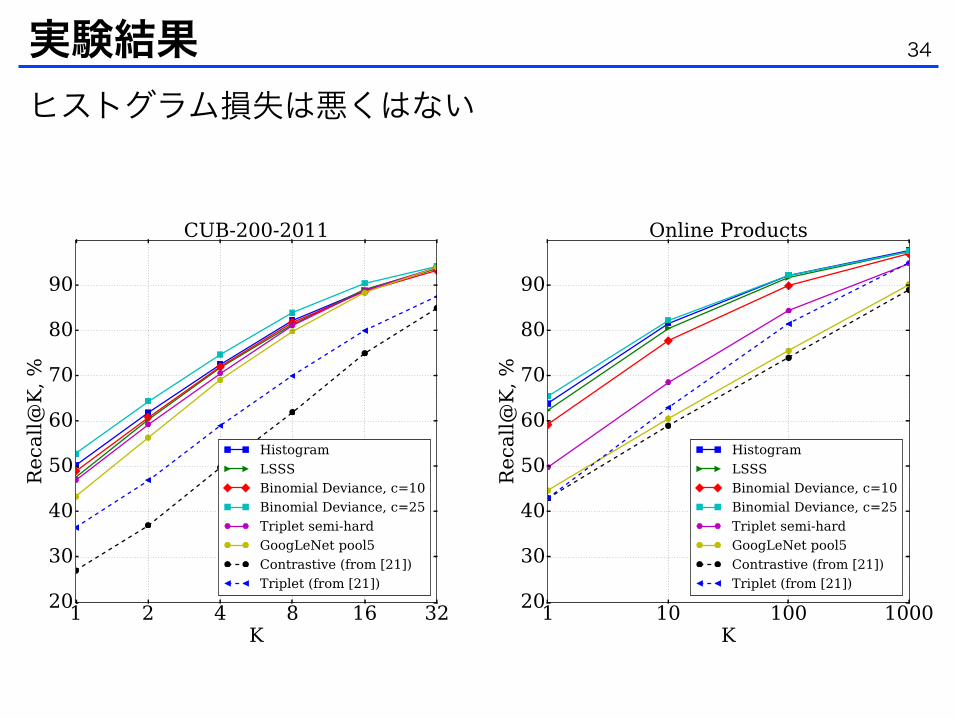
Figure 3: Recall@K for (left) - CUB-200-2011 and (right) - Online Products datasets for different methods.Results for the Histogram loss (4), Binomial Deviance (7), LSSS [21] and Triplet [18] losses are present.Binomial Deviance loss for C = 25 outperforms all other methods. The best-performing method is Histogramloss. We also include results for contrastive and triplet losses from [21].
Datasets and evaluation metrics. We have evaluated the above mentioned loss functions on thefour datasets : CUB200-2011 [25], CUHK03 [11], Market-1501 [29] and Online Products [21]. Allthese datasets have been used for evaluating methods of solving embedding learning tasks.
The CUB-200-2011 dataset includes 11,788 images of 200 classes corresponding to different birdsspecies. As in [21] we use the first 100 classes for training (5,864 images) and the remaining classesfor testing (5,924 images). The Online Products dataset includes 120,053 images of 22,634 classes.Classes correspond to a number of online products from eBay.com. There are approximately 5.3images for each product. We used the standard split from [21]: 11,318 classes (59,551 images) areused for training and 11,316 classes (60,502 images) are used for testing. The images from theCUB-200-2011 and the Online Products datasets are resized to 256 by 256, keeping the originalaspect ratio (padding is done when needed).
The CUHK03 dataset is commonly used for the person re-identification task. It includes 13,164images of 1,360 pedestrians captured from 3 pairs of cameras. Each identity is observed by twocameras and has 4.8 images in each camera on average. Following most of the previous works we usethe “CUHK03-labeled” version of the dataset with manually-annotated bounding boxes. Accordingto the CUHK03 evaluation protocol, 1,360 identities are split into 1,160 identities for training, 100for validation and 100 for testing. We use the first split from the CUHK03 standard split set which isprovided with the dataset. The Market-1501 dataset includes 32,643 images of 1,501 pedestrians,each pedestrian is captured by several cameras (from two to six). The dataset is divided randomlyinto the test set of 750 identities and the train set of 751 identities.
Following [21; 27; 29], we report Recall@K1 metric for all the datasets. For CUB-200-2011 andOnline products, every test image is used as the query in turn and remaining images are used as thegallery correspondingly. In contrast, for CUHK03 single-shot results are reported. This means thatone image for each identity from the test set is chosen randomly in each of its two camera views.Recall@K values for 100 random query-gallery sets are averaged to compute the final result for agiven split. For the Market-1501 dataset, we use the multi-shot protocol (as is done in most otherworks), as there are many images of the same person in the gallery set.
Architectures used. For training on the CUB-200-2011 and the Online Products datasets we usedthe same architecture as in [21], which conincides with the GoogleNet architecture [23] up to the‘pool5’ and the inner product layers, while the last layer is used to compute the embedding vectors.The GoogleNet part is pretrained on ImageNet ILSVRC [16] and the last layer is trained from scratch.As in [21], all GoogLeNet layers are fine-tuned with the learning rate that is ten times less than
1Recall@K is the probability of getting the right match among first K gallery candidates sorted by similarity.
6

Figure 4: Recall@K for (left) - CUHK03 and (right) - Market-1501 datasets. The Histogram loss (4) outperformsBinomial Deviance, LSSS and Triplet losses.
the learning rate of the last layer. We set the embedding size to 512 for all the experiments withthis architecture. We reproduced the results for the LSSS loss [21] for these two datasets. For thearchitectures that use the Binomial Deviance loss, Histogram loss and Triplet loss the iteration numberand the parameters value (for the former) are chosen using the validation set.
For training on CUHK03 and Market-1501 we used the Deep Metric Learning (DML) architectureintroduced in [27]. It has three CNN streams for the three parts of the pedestrian image (head andupper torso, torso, lower torso and legs). Each of the streams consists of 2 convolution layers followedby the ReLU non-linearity and max-pooling. The first convolution layers for the three streams haveshared weights. Descriptors are produced by the last 500-dimensional inner product layer that has theconcatenated outputs of the three streams as an input.
Table 1: Final results for CUHK03-labeled and Market-1501. ForCUHK03-labeled results for 5 random splits were averaged. Batchof size 256 was used for both experiments.
Dataset r = 1 r = 5 r = 10 r = 15 r = 20
CUHK03 65.77 92.85 97.62 98.94 99.43Market-1501 59.47 80.73 86.94 89.28 91.09
Implementation details. For all theexperiments with loss functions (4)and (7) we used quadratic numberof pairs in each batch (all the pairsthat can be sampled from batch). Fortriplet loss “semi-hard” triplets cho-sen from all the possible triplets in thebatch are used. For comparison withother methods the batch size was setto 128. We sample batches randomlyin such a way that there are several
images for each sampled class in the batch. We iterate over all the classes and all the imagescorresponding to the classes, sampling images in turn. The sequences of the classes and of thecorresponding images are shuffled for every new epoch. CUB-200-2011 and Market-1501 includemore than ten images per class on average, so we limit the number of images of the same class in thebatch to ten for the experiments on these datasets. We used ADAM [7] for stochastic optimizationin all of the experiments. For all losses the learning rate is set to 1e � 4 for all the experimentsexcept ones on the CUB-200-2011 datasets, for which we have found the learning rate of 1e � 5
more effective. For the re-identification datasets the learning rate was decreased by 10 after the 100Kiterations, for the other experiments learning rate was fixed. The iterations number for each methodwas chosen using the validation set.
Results. The Recall@K values for the experiments on CUB-200-2011, Online Products, CUHK03and Market-1501 are shown in Figure 3 and Figure 4. The Binomial Deviance loss (7) gives thebest results for CUB-200-2011 and Online Products with the C parameter set to 25. We previouslychecked several values of C on the CUB-200-2011 dataset and found the value C = 25 to be theoptimal one. We also observed that with smaller values of C the results are significantly worse than
7

l
l


Quadruplet-wise Image Similarity Learning
Marc T. Law Nicolas Thome Matthieu Cord
LIP6, UPMC - Sorbonne University, Paris, France{Marc.Law, Nicolas.Thome, Matthieu.Cord}@lip6.fr
Abstract
This paper introduces a novel similarity learning frame-work. Working with inequality constraints involvingquadruplets of images, our approach aims at efficientlymodeling similarity from rich or complex semantic labelrelationships. From these quadruplet-wise constraints, wepropose a similarity learning framework relying on a con-vex optimization scheme. We then study how our metriclearning scheme can exploit specific class relationships,such as class ranking (relative attributes), and class tax-onomy. We show that classification using the learned met-rics gets improved performance over state-of-the-art meth-ods on several datasets. We also evaluate our approachin a new application to learn similarities between webpagescreenshots in a fully unsupervised way.
1. IntroductionSimilarity learning is useful in many Computer Vision
applications, such as image classification [6, 10, 17], imageretrieval [6], face verification or person re-identification [12,18]. The key ingredients of similarity learning frameworkare (i) the data representation including both the featurespace and the similarity function, (ii) the learning frame-work which includes: training data, type of labels and rela-tions, the optimization formulation and solvers.
The usual way to learn similarities is to consider binarylabels on image pairs [29]. For instance, in the context offace verification [12], binary labels establish whether twoimages should be considered equivalent or not. Metrics arelearned with training data to minimize dissimilarities be-tween similar pairs while separating dissimilar ones. Manydifferent metrics have been considered in Euclidean spaceor using kernel embedding [18].
Recently, some attempts have been made to go be-yond learning metrics with pairwise constraints generatedfrom binary class membership labels. On the one hand,triplet-wise constraints have been considered to learn met-rics [6, 15, 28]. Triplet constraints may be generated from
Presence of smile− +
Least smiling≺ ? ∼ ? ≺Most smiling
Class (e) Class (f ) Class (g) Class (h)! "# $
⇓Learn dissimilarity D such that:
D( , ) < D( , )
D( , ) < D( , )
Figure 1. Quadruplet-wise (Qwise) strategy on 4 face classesranked according to the degree of presence of smile. Instead ofworking on pairwise relations that present some flaws (see text),Qwise strategy defines quadruplet-wise constraints to express thatdissimilarities between examples from (f ) and (g) should besmaller than dissimilarities between examples from (e) and (h).
class labels or they can be inferred from richer relationships.For example, Verma et al. [26] learn a similarity that de-pends on a class hierarchy: an image should be closer toanother image from a sibling class than to any image from adistant class in the hierarchy. Other methods exploit spe-cific rankings between classes. For instance, relative at-tributes have been introduced in [20]: different classes (e.g.”celebrity”) are ranked with respect to different concepts orattributes (e.g. ”smile”), see Fig. 1 (top). Pairwise relationsare extracted: e.g. face images from class (x) smile morethan (or as much as) face images from class (y). In [20],it is shown that learning relative features can help signifi-cantly boost classification performances.
In this paper, we focus on these rich contexts for learningsimilarity metrics. Instead of pairwise or triplet-wise tech-niques, we propose to investigate relations between quadru-plets of images. We claim that, in many contexts, consider-
2013 IEEE International Conference on Computer Vision
1550-5499/13 $31.00 © 2013 IEEEDOI 10.1109/ICCV.2013.38
249
2013 IEEE International Conference on Computer Vision
1550-5499/13 $31.00 © 2013 IEEEDOI 10.1109/ICCV.2013.38
249