learning goal-directed behaviour
TRANSCRIPT

IN DEGREE PROJECT COMPUTER SCIENCE AND ENGINEERING,SECOND CYCLE, 30 CREDITS
, STOCKHOLM SWEDEN 2017
Learning Goal-Directed Behaviour
MARCEL BINZ
KTH ROYAL INSTITUTE OF TECHNOLOGYSCHOOL OF COMPUTER SCIENCE AND COMMUNICATION

Learning Goal-Directed Behaviour
MARCEL BINZ
Master in Machine Learning
Date: June 14, 2017
Supervisor: Florian Pokorny
Examiner: Danica Kragic
School of Computer Science and Communication
i
Abstract
Learning behaviour of artificial agents is commonly studied in the framework of Rein-
forcement Learning. Reinforcement Learning gained increasing popularity in the past
years. This is partially due to developments that enabled the possibility to employ com-
plex function approximators, such as deep networks, in combination with the frame-
work. Two of the core challenges in Reinforcement Learning are the correct assignment
of credits over long periods of time and dealing with sparse rewards. In this thesis we
propose a framework based on the notions of goals to tackle these problems. This work
implements several components required to obtain a form of goal-directed behaviour,
similar to how it is observed in human reasoning. This includes the representation of a
goal space, learning how to set goals and finally how to reach them. The framework it-
self is build upon the options model, which is a common approach for representing tem-
porally extended actions in Reinforcement Learning. All components of the proposed
method can be implemented as deep networks and the complete system can be learned
in an end-to-end fashion using standard optimization techniques. We evaluate the ap-
proach on a set of continuous control problems of increasing difficulty. We show, that we
are able to solve a difficult gathering task, which poses a challenge to state-of-the-art Re-
inforcement Learning algorithms. The presented approach is furthermore able to scale to
complex kinematic agents of the MuJoCo benchmark.
ii
Sammanfattning
Inlärning av beteende för artificiella agenter studeras vanligen inom Reinforcement Le-
arning. Reinforcement Learning har på senare tid fått ökad uppmärksamhet, detta beror
delvis på utvecklingen som gjort det möjligt att använda komplexa funktionsapproxi-
merare, såsom djupa nätverk, i kombination med Reinforcement Learning. Två av kär-
nutmaningarna inom reinforcement learning är credit assignment-problemet över långa
perioder samt hantering av glesa belöningar. I denna uppsats föreslår vi ett ramverk ba-
serat på delvisa mål för att hantera dessa problem. Detta arbete undersöker de kompo-
nenter som krävs för att få en form av målinriktat beteende, som liknar det som obser-
veras i mänskligt resonemang. Detta inkluderar representation av en målrymd, inlärning
av målsättning, och till sist inlärning av beteende för att nå målen. Ramverket bygger
på options-modellen, som är ett gemensamt tillvägagångssätt för att representera tempo-
ralt utsträckta åtgärder inom Reinforcement Learning. Alla komponenter i den föreslagna
metoden kan implementeras med djupa nätverk och det kompletta systemet kan tränas
end-to-end med hjälp av vanliga optimeringstekniker. Vi utvärderar tillvägagångssättet
på en rad kontinuerliga kontrollproblem med varierande svårighetsgrad. Vi visar att vi
kan lösa en utmanande samlingsuppgift, som tidigare state-of-the-art algoritmer har upp-
visat svårigheter för att hitta lösningar. Den presenterade metoden kan vidare skalas upp
till komplexa kinematiska agenter i MuJoCo-simuleringar.
Contents
Contents iii
1 Introduction 2
2 Related Work 4
2.1 Feudal Reinforcement Learning . . . . . . . . . . . . . . . . . . . . . . . . . . . 4
2.2 Option Discovery . . . . . . . . . . . . . . . . . . . . . . . . . . . . . . . . . . . 5
2.3 Universal Value Function Approximators . . . . . . . . . . . . . . . . . . . . . 5
2.4 Alternative Hierarchical Approaches . . . . . . . . . . . . . . . . . . . . . . . . 6
2.5 Intrinsic Motivation . . . . . . . . . . . . . . . . . . . . . . . . . . . . . . . . . . 6
3 Preliminaries 7
3.1 Reinforcement Learning . . . . . . . . . . . . . . . . . . . . . . . . . . . . . . . 8
3.1.1 Markov Decision Processes . . . . . . . . . . . . . . . . . . . . . . . . . 8
3.1.2 Monte-Carlo Methods . . . . . . . . . . . . . . . . . . . . . . . . . . . . 10
3.1.3 Temporal-Difference Learning . . . . . . . . . . . . . . . . . . . . . . . 10
3.1.4 Policy Gradients Theorem . . . . . . . . . . . . . . . . . . . . . . . . . . 11
3.1.5 Asynchronous Advantage Actor-Critic (A3C) . . . . . . . . . . . . . . 12
3.2 Function Approximation with Neural Networks . . . . . . . . . . . . . . . . . 14
3.2.1 Feed-forward Neural Networks . . . . . . . . . . . . . . . . . . . . . . 14
3.2.2 Recurrent Neural Networks . . . . . . . . . . . . . . . . . . . . . . . . 15
3.2.3 Gradient-Based Learning . . . . . . . . . . . . . . . . . . . . . . . . . . 16
3.2.4 Attention Mechanisms . . . . . . . . . . . . . . . . . . . . . . . . . . . . 17
3.3 Hierarchical Reinforcement Learning . . . . . . . . . . . . . . . . . . . . . . . 19
3.3.1 Options Framework . . . . . . . . . . . . . . . . . . . . . . . . . . . . . 19
3.3.2 Universal Value Function Approximators . . . . . . . . . . . . . . . . 19
4 Methods 21
4.1 Hierarchical Reinforcement Learning with Goals . . . . . . . . . . . . . . . . 21
4.1.1 Motivation . . . . . . . . . . . . . . . . . . . . . . . . . . . . . . . . . . . 22
4.1.2 Goal-Setting Policy . . . . . . . . . . . . . . . . . . . . . . . . . . . . . . 23
4.1.3 Goal-Reaching Policy . . . . . . . . . . . . . . . . . . . . . . . . . . . . 24
4.1.4 Interpretation as Options . . . . . . . . . . . . . . . . . . . . . . . . . . 25
4.2 Connections to Related Approaches . . . . . . . . . . . . . . . . . . . . . . . . 25
iii
iv CONTENTS
5 Experiments 26
5.1 Randomized Goals with Fixed Embeddings . . . . . . . . . . . . . . . . . . . 28
5.1.1 Task . . . . . . . . . . . . . . . . . . . . . . . . . . . . . . . . . . . . . . 28
5.1.2 Experimental Details . . . . . . . . . . . . . . . . . . . . . . . . . . . . . 28
5.1.3 Results . . . . . . . . . . . . . . . . . . . . . . . . . . . . . . . . . . . . . 29
5.1.4 Discussion . . . . . . . . . . . . . . . . . . . . . . . . . . . . . . . . . . . 30
5.2 Learned Goals with Fixed Embeddings . . . . . . . . . . . . . . . . . . . . . . 32
5.2.1 Task . . . . . . . . . . . . . . . . . . . . . . . . . . . . . . . . . . . . . . 32
5.2.2 Experimental Details . . . . . . . . . . . . . . . . . . . . . . . . . . . . . 33
5.2.3 Results . . . . . . . . . . . . . . . . . . . . . . . . . . . . . . . . . . . . . 35
5.2.4 Discussion . . . . . . . . . . . . . . . . . . . . . . . . . . . . . . . . . . . 35
5.3 Learned Goals with Learned Embeddings . . . . . . . . . . . . . . . . . . . . 38
5.3.1 Task . . . . . . . . . . . . . . . . . . . . . . . . . . . . . . . . . . . . . . 38
5.3.2 Experimental Details . . . . . . . . . . . . . . . . . . . . . . . . . . . . . 38
5.3.3 Results . . . . . . . . . . . . . . . . . . . . . . . . . . . . . . . . . . . . . 39
5.3.4 Discussion . . . . . . . . . . . . . . . . . . . . . . . . . . . . . . . . . . . 40
6 Conclusion and Future Work 42
Bibliography 44
Notation
We provide a short summary of the notation used in this thesis. In general vectors are
denoted with small, bold and matrices with large, bold letters.
st Observation at time step t
at Action at time step t
zt Activation in goal space at time step t
gt Goal at time step t
ht Hidden state of a neural network at time step t
S Observation space
A Action space
G Goal space
p(st+1|st,at) Transition probability
rt Reward at time step t
Rt Return following time step t
V π(s) State value function of state s when following policy π
Qπ(s,a) Action value function of state s and action a when following policy π
Aπ(s,a) Advantage function of state s and action a when following policy π
π Policy
φ Goal embedding
Ω Set of all available options
ω Single option from Ω
α Learning rate
β Entropy scaling factor
γ Discount factor
θ Set of parameters being learned
τ Trajectory of states and actions
W Weight matrix of neural network layer
b Bias vector of neural network layer
y Targets from supervised learning
y Predictions corresponding to y
E[•] Expectation of a random variable
(•)S Subscript referring to goal-setting policy
(•)R Subscript referring to goal-reaching policy
1
Chapter 1
Introduction
Being able to build computational agents, that can perform complex tasks in unknown
environments, is of enormous value for our society. In general we would like to enable
such systems to learn their behaviour from experience, as defining them explicitly is of-
ten impossible. Reinforcement Learning (RL) provides a general mathematical framework
to model such agents. Recent advances in RL, in particular its combination with methods
from Deep Learning, allowed these methods to scale to much more challenging problems.
These problem include, amongst others, playing ATARI 2600 games [1], robotic manipu-
lation [2] and mastering the game of Go [3].
Two of the key challenges in Reinforcement Learning are proper credit assignment
over long periods of time and dealing with sparse rewards. To highlight these prob-
lems, let us inspect the results reported for different games of the well-established ATARI
2600 benchmark [4]. Here we notice that state-of-the-art methods [1, 5] are able to solve
most reactive games, such as Ping-Pong or Breakout, easily. However games, that require
long term planning and abstract reasoning, such as Montezuma’s Revenge, pose a much
harder challenge for these algorithms.
Hierarchical Reinforcement Learning attempts to deal with these challenges by de-
composing the problem into smaller sub-tasks, which are then solved independently.
There are different ways how this decomposition is realized and we will review some of
these in the later parts of this thesis. In this work we will focus on a form of hierarchical
RL, that is based on the notion of goals.
For this we will describe a framework, that exhibits a form of goal-directed behaviour.
In our approach we strive for as much generality as possible, meaning that all compo-
nents should be learned from interaction with the world. These components include:
1. Learning the structure of a goal space
2. Setting goals on given space
3. Reaching those goals through atomic actions
During the stages of this thesis we will relax some of the generality assumptions in order
to build up an incremental solution, that tackles all three components, required to attain
goal-directed behaviour.
2
CHAPTER 1. INTRODUCTION 3
It may not be directly obvious, how to define goals in mathematical terms. It is how-
ever important to provide such a definition in order to implement the described mechan-
ics. For our purposes goals are elements of an abstract goal space, such as vector spaces.
These representations may be specified by the human designer or correspond to hidden
states of deep network. In general it is required, that the agent can interfere its current
position in goal space, decide where it would like to be and is able perform actions to
minimize the discrepancy between current position and goal.
Let us consider a few examples to be more concrete about this concept and highlight
its potential advantages. In the first scenario our task is to maneuver an ant-like robot
through a maze, and we are only rewarded for reaching the exit. While we have to learn
about complex behaviour sequences to control the robot, the reward structure of the task
depends only on its location in the maze. Therefore it is natural to consider a decom-
position based on goals. Here the goal space could correspond to locations in the maze,
which the robot would like to reach. For other tasks it may be desirable to exhibit more
complex structures. In an ego-shooter game goals could, in addition to moving to cer-
tain locations, correspond to high-level events, such as a kill on an opponent or collect-
ing new weapons.
Reasoning about goals could provide means for more structured exploration in com-
plex problems. This is especially important in tasks with sparse or even non-existing re-
wards. Such settings are challenging for the current RL approaches, as these only per-
form exploration through sampling from stochastic policies, such as a Boltzmann distri-
bution, for discrete actions, or Gaussian distributions in the continuous case. However in
many tasks adding this kind of noise will never lead to meaningful action sequences.
Both, Reinforcement and Deep Learning, are to some extent inspired by how humans
learn to represent and solve problems. In similar fashion we also observe forms of goal-
directed reasoning in human behaviour. Indeed psychologists and cognitive scientist of-
ten distinguish between two types of behaviour – habitual and goal-directed [6, 7]. There
are also links to neuroscience, where for example the neurotransmitter Dopamine is be-
lieved to regulate goal-directed behavior [8] in the human brain. For a recent overview of
connections between hierarchical RL, psychology and neuroscience we refer the reader to
[9].
The main contributions in the presented work are the proposal and implementation
of a framework for end-to-end learning of goal-directed behaviour, its application to con-
tinuous control problems and investigation of different properties through experiments.
The remainder of this thesis is structured as follows. First we provide a broad overview
of related work in Chapter 2. This is followed in Chapter 3 by presenting important pre-
supposed techniques. Chapter 4 outlines the proposed framework and motivates its spe-
cific design choices. It also places the suggested technique in the context of similar ap-
proaches. We validate the approach in Chapter 5 through a set of experiments with in-
creasing difficulty. This chapter also includes an analysis of the obtained results. We con-
clude this thesis in Chapter 6.
Chapter 2
Related Work
A major part of the work presented in this thesis is based on the ability to apply Rein-
forcement Learning techniques in high-dimensional, continuous observation and action
spaces. In these cases it is natural to employ complex function approximators such as
deep networks. Combining these two methods proves however challenging due to sta-
bility problems during the learning process. Recent work in Deep Q-Networks (DQN) [1]
showed how to overcome these issues when dealing with discrete actions. Since then
these methods have been extended to the case of continuous control. Here we make ex-
tensive use of A3C [5], which is an on-policy actor-critic algorithm. There is however a
wide range of other algorithms that could be applied instead, such as continuous DQN
variants [10], Trust Region Policy Optimization [11], off-policy actor-critics [12, 13] or meth-
ods with deterministic policies [14, 15].
A3C itself has been extended in several ways. Generalized Advantage Estimation [16]
can be employed as a technique to control bias and variance in the estimation of the ad-
vantage function. [12] proposes a fast and flexible trust region update method, which
was tested empirically in combination with A3C. UNREAL [17] adds a set of unsuper-
vised auxiliary tasks on top of A3C and show significant improvement in stability, speed
and performance.
The tasks we consider in this report are based on the MuJoCo physics simulator [18]
and have been proposed in [19]. Since they have been used in several research papers.
2.1 Feudal Reinforcement Learning
Hierarchical Reinforcement Learning is an area of diverse approaches. Out of all these
Feudal Reinforcement Learning (FRL) [20] resembles the model proposed in this thesis the
most. FRL is based on the metaphor of the hierarchical aspects of feudal fiefdom. It de-
fines a framework consisting of a hierarchy of managers, in which higher ones are able
to set sub-tasks for lower ones. Recently two models have been proposed, which com-
bine FRL with deep networks [21, 22]. The former [21] has been applied to the chal-
lenging ATARI 2600 game Montezuma’s Revenge. It uses a two-level DQN hierarchy,
in which the higher one operates over a hand-designed space of entities and relations.
[22] design an end-to-end trainable model, that fits the FRL framework and learns its
high-level goal space jointly with the task. Their model is evaluated on a set of challeng-
ing ATARI 2600 games, where it performs favorable against rivaling approaches. Also
4
CHAPTER 2. RELATED WORK 5
in this line of work is the HASSLE [23] algorithm, in which a high level policy selects a
sub-goal from a set of abstract high-level observations, which is obtained through an un-
supervised vector quantization technique. Low-level polices are governed with reaching
these goals. In their case a limited set of low-level polices learns to associate itself auto-
matically with the most-suitable high-level observations. Recently a related model has
been applied to continuous action spaces, where a simulated biped robot learns to drib-
ble a soccer ball and to navigate through static as well as dynamic obstacles [24].
2.2 Option Discovery
The options framework [25] is a popular choice for modelling temporal abstractions in
RL. An option is defined as a temporally extended sequence of actions with a termina-
tion criterion. As the framework itself does not describe how options arise, there is large
amount of additional methods for learning them from experience. Identifying suitable
sub-goals is often the first step when constructing options. Given this connection to goal-
directed behaviour, we will briefly review some methods for option discovery in the fol-
lowing.
In the given setting Machado et al. propose to identify purposes, that are just out of
reach [26]. This is archived through the use of singular value decomposition on changes
in consecutive observations of the environment. The result is then transformed into sub-
goals, which are learned through an intrinsic reward function. A related approach is
taken in [27], where PCCA+ is used to perform a spectral clustering of the MDP.
A similar concept was proposed by the authors of [28]. Their approach relies on iden-
tifying bottlenecks in the observation space. In their case a bottleneck is defined as a
state, that is visited on many successful paths (such as a doorway). Discovered states are
than turned into options through a learned policy based on an intrinsic reward function.
The optic-critic architecture [29] extends the policy gradient theorem to options. This
allows to jointly learn internal policies along with policies over options. The approach is
appealing as it only requires to specify the number of options, but no intrinsic rewards
or sub-goals.
2.3 Universal Value Function Approximators
How do we provide the agent with information about which sub-goal it currently tries
to reach? Most of the outlined approaches in this section learn an independent policy for
each possible sub-goal. Universal Value Function Approximators (UVFA) [30] on the other
hand provide the ability to treat sub-goals as a part of the observation. This enables to
generalize between different sub-goals and allows, in theory, to employ infinite sets of
them.
UVFAs have been applied to several settings, that include hand-designed, high-level
goals. This includes visual navigation of robots [31, 32], where goals are locations on a
map and first-person shooter games [33], where goals correspond to maximization of dif-
ferent game measurements (such as health, ammunition or kill score).
6 CHAPTER 2. RELATED WORK
2.4 Alternative Hierarchical Approaches
There is also a large set of alternative approaches to hierarchical Reinforcement Learning
besides those, that are based on sub-goals and options. The MAXQ value function de-
composition [34] decomposes the original MDP into a set of smaller MDPs in a way, that
the original value function is transformed into an additive combination of the new ones.
For this the programmer has to identify and define useful sub-tasks in advance.
The Hierarchy of Abstract Machines [35] model is build upon a set of non-deterministic
finite state machines, whose transition can trigger machines at lower levels. This setup
constrains the actions, that the agent can take in each state, allowing to incorporate prior
knowledge into the task at hand.
Macro-actions are simpler instance of options, where whole action sequences are de-
cided at the point of their initiation. They have been proposed in [36], and since then
been investigated in other works such as [37]. STRAW [38] consists of a deep network,
that maintains a plan in form of macro-actions. This plan can be adjusted on certain
re-planning points. The whole model is trainable end-to-end and does not require any
pseudo-rewards or additional hand-crafted information.
The Horde architecture [39] shows many similarities to the approach presented in this
work. It consists of a large number of sub-agents, called demons. Each of the demons
has its own policy and is responsible for answering a single goal-oriented question. These
questions are posed in form of different value functions. The whole system runs many
demons in parallel, similar to how A3C is used in this thesis.
2.5 Intrinsic Motivation
Employing goal-based methods provides a mechanism for structured exploration of the
environment. This objective however can also be realized through other means. It is of-
ten investigated through the lens of intrinsic motivation. Here one strategy is to place a
bonus reward, based on visitation statistics of states [40]. This bonus then encourages to
visit states, which have not been seen before. Recently techniques have been proposed,
that are based on hashing [41] or density models [42, 43] to keep track of the visitation
counter in continuous state spaces.
Yet another approach to obtain intrinsic motivation is via uncertainties in predic-
tions. For example we can model uncertainties with a Bayesian model [44] and than use
Thompson sampling [45] to exploit them for exploration. Another alternative is to max-
imize the reduction in uncertainty of a dynamics models via the mutual information be-
tween the next state distribution and the model parameters [46] or to use surprise-based
mechanisms [47, 48].
Chapter 3
Preliminaries
To allow computational agents to adapt their behaviour based on experience, we first
need to establish the mathematical foundations of interacting within an environment.
Different aspects of this process will be presented within this chapter.
The first part provides an overview over the theory of Reinforcement Learning (RL)
as it is employed in later parts of this report. First the framework will be outlined and
several of its properties will be highlighted. We then continue to describe how decisions
can be modelled within the framework as Markov Decision Processes (MDP). This section
will also define the quantities, which should be optimized in order to learn desired be-
haviour. Most Reinforcement Learning methods alternate in some way between estimat-
ing the quality of the current behaviour in terms of value functions, followed by improv-
ing given behaviour. We present the two major techniques for learning to estimate value
functions, namely Monte-Carlo methods and Temporal-Difference learning. Finally we
will show how the obtained estimates can be used to update the agents actions via the
policy gradient theorem.
Traditional RL methods rely on table-based methods to keep track of their prior ex-
perience. These methods are however not applicable in high-dimensional, continuous
spaces. Here one can instead resort to (parametrized) function approximators. In this
setting neural networks1 are a popular choice due their ability to learn arbitrary func-
tions under mild assumptions [49, 50]. As part of this chapter we will define both feed-
forward and recurrent neural network models and show how these can learn from data
using gradient-based updates.
We will conclude this chapter with a section on hierarchical Reinforcement Learning.
For this we will outline the options framework [25], which allows to incorporate high-
level primitives into the traditional RL framework. We will also highlight a connection
between options and semi-Markov Decision Processes, which allows to transfer some
theoretical guarantees for traditional RL to its hierarchical counterpart. Finally we will
present Universal Value Function Approximators (UVFA), which enable generalization be-
tween a – possibly infinite – set of options.
1In this thesis we use the terms neural network and deep network interchangeably.
7
8 CHAPTER 3. PRELIMINARIES
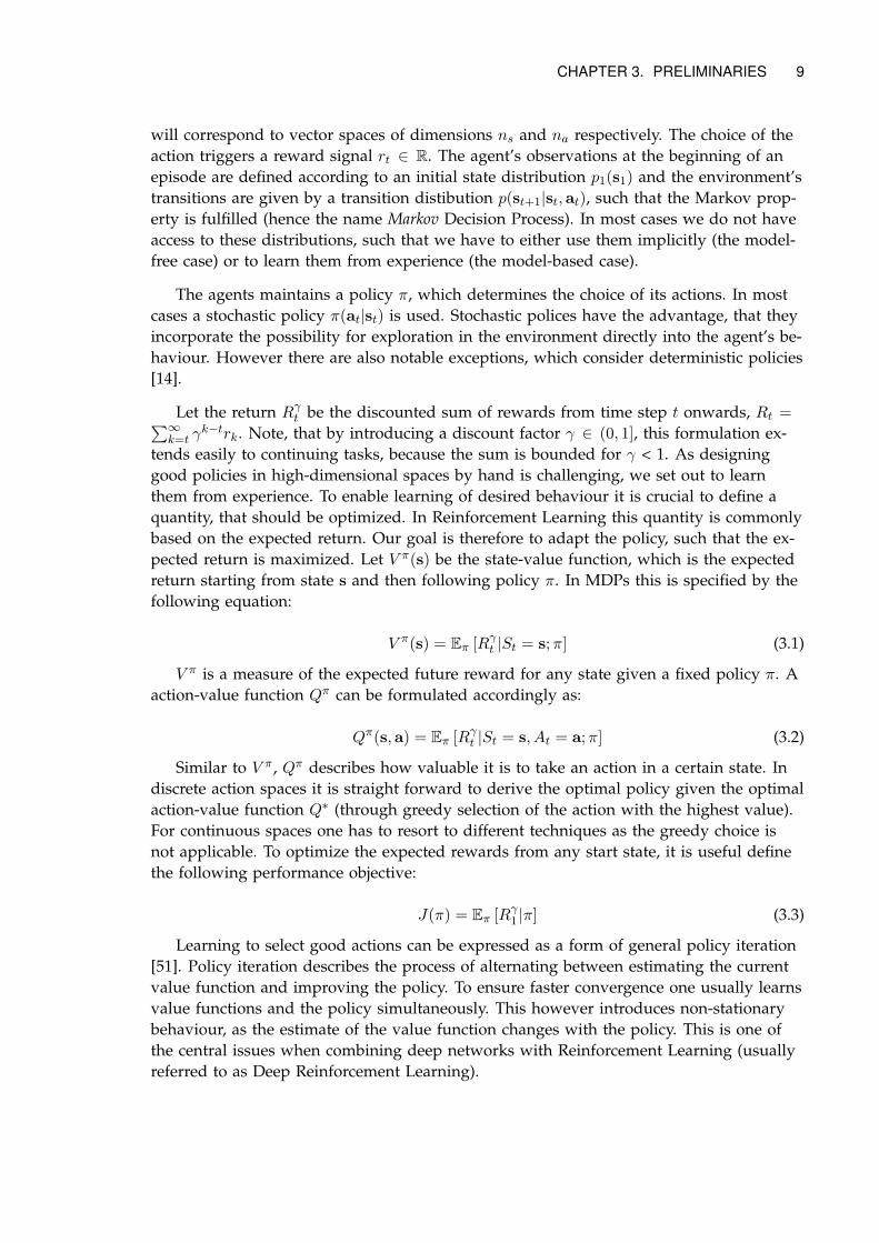
Agent Environment
action
observation, reward
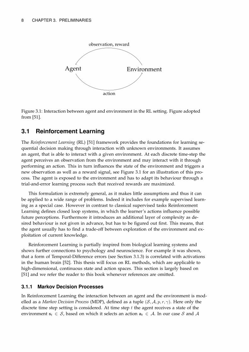
Figure 3.1: Interaction between agent and environment in the RL setting. Figure adopted
from [51].
3.1 Reinforcement Learning
The Reinforcement Learning (RL) [51] framework provides the foundations for learning se-
quential decision making through interaction with unknown environments. It assumes
an agent, that is able to interact with a given environment. At each discrete time-step the
agent perceives an observation from the environment and may interact with it through
performing an action. This in turn influences the state of the environment and triggers a
new observation as well as a reward signal, see Figure 3.1 for an illustration of this pro-
cess. The agent is exposed to the environment and has to adapt its behaviour through a
trial-and-error learning process such that received rewards are maximized.
This formulation is extremely general, as it makes little assumptions and thus it can
be applied to a wide range of problems. Indeed it includes for example supervised learn-
ing as a special case. However in contrast to classical supervised tasks Reinforcement
Learning defines closed loop systems, in which the learner’s actions influence possible
future perceptions. Furthermore it introduces an additional layer of complexity as de-
sired behaviour is not given in advance, but has to be figured out first. This means, that
the agent usually has to find a trade-off between exploration of the environment and ex-
ploitation of current knowledge.
Reinforcement Learning is partially inspired from biological learning systems and
shows further connections to psychology and neuroscience. For example it was shown,
that a form of Temporal-Difference errors (see Section 3.1.3) is correlated with activations
in the human brain [52]. This thesis will focus on RL methods, which are applicable to
high-dimensional, continuous state and action spaces. This section is largely based on
[51] and we refer the reader to this book whenever references are omitted.
3.1.1 Markov Decision Processes
In Reinforcement Learning the interaction between an agent and the environment is mod-
elled as a Markov Decision Process (MDP), defined as a tuple (S,A, p, r, γ). Here only the
discrete time step setting is considered. At time step t the agent receives a state of the
environment st ∈ S , based on which it selects an action at ∈ A. In our case S and A
CHAPTER 3. PRELIMINARIES 9
will correspond to vector spaces of dimensions ns and na respectively. The choice of the
action triggers a reward signal rt ∈ R. The agent’s observations at the beginning of an
episode are defined according to an initial state distribution p1(s1) and the environment’s
transitions are given by a transition distibution p(st+1|st,at), such that the Markov prop-
erty is fulfilled (hence the name Markov Decision Process). In most cases we do not have
access to these distributions, such that we have to either use them implicitly (the model-
free case) or to learn them from experience (the model-based case).
The agents maintains a policy π, which determines the choice of its actions. In most
cases a stochastic policy π(at|st) is used. Stochastic polices have the advantage, that they
incorporate the possibility for exploration in the environment directly into the agent’s be-
haviour. However there are also notable exceptions, which consider deterministic policies
[14].
Let the return Rγt be the discounted sum of rewards from time step t onwards, Rt =
∑
∞
k=t γk−trk. Note, that by introducing a discount factor γ ∈ (0, 1], this formulation ex-
tends easily to continuing tasks, because the sum is bounded for γ < 1. As designing
good policies in high-dimensional spaces by hand is challenging, we set out to learn
them from experience. To enable learning of desired behaviour it is crucial to define a
quantity, that should be optimized. In Reinforcement Learning this quantity is commonly
based on the expected return. Our goal is therefore to adapt the policy, such that the ex-
pected return is maximized. Let V π(s) be the state-value function, which is the expected
return starting from state s and then following policy π. In MDPs this is specified by the
following equation:
V π(s) = Eπ [Rγt |St = s;π] (3.1)
V π is a measure of the expected future reward for any state given a fixed policy π. A
action-value function Qπ can be formulated accordingly as:
Qπ(s,a) = Eπ [Rγt |St = s, At = a;π] (3.2)
Similar to V π, Qπ describes how valuable it is to take an action in a certain state. In
discrete action spaces it is straight forward to derive the optimal policy given the optimal
action-value function Q∗ (through greedy selection of the action with the highest value).
For continuous spaces one has to resort to different techniques as the greedy choice is
not applicable. To optimize the expected rewards from any start state, it is useful define
the following performance objective:
J(π) = Eπ [Rγ1 |π] (3.3)
Learning to select good actions can be expressed as a form of general policy iteration
[51]. Policy iteration describes the process of alternating between estimating the current
value function and improving the policy. To ensure faster convergence one usually learns
value functions and the policy simultaneously. This however introduces non-stationary
behaviour, as the estimate of the value function changes with the policy. This is one of
the central issues when combining deep networks with Reinforcement Learning (usually
referred to as Deep Reinforcement Learning).
10 CHAPTER 3. PRELIMINARIES
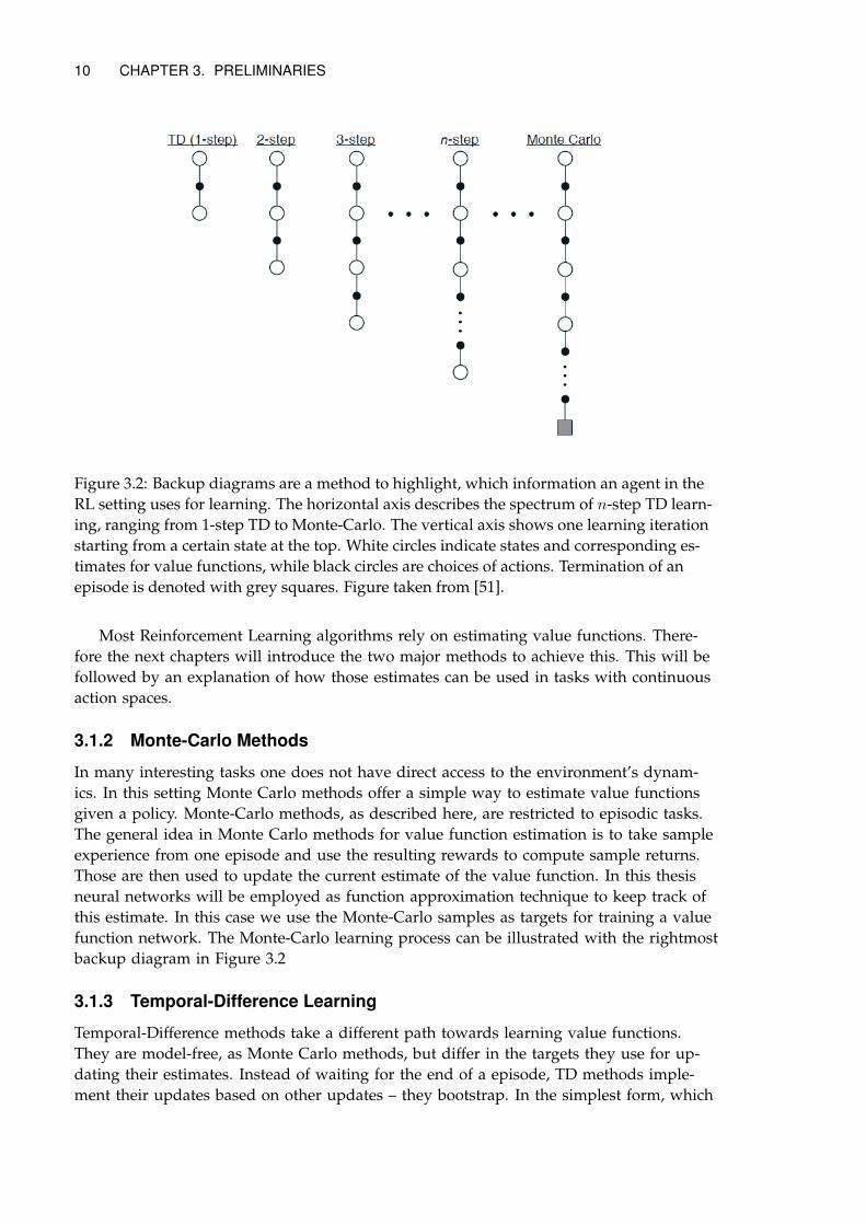
Figure 3.2: Backup diagrams are a method to highlight, which information an agent in the
RL setting uses for learning. The horizontal axis describes the spectrum of n-step TD learn-
ing, ranging from 1-step TD to Monte-Carlo. The vertical axis shows one learning iteration
starting from a certain state at the top. White circles indicate states and corresponding es-
timates for value functions, while black circles are choices of actions. Termination of an
episode is denoted with grey squares. Figure taken from [51].
Most Reinforcement Learning algorithms rely on estimating value functions. There-
fore the next chapters will introduce the two major methods to achieve this. This will be
followed by an explanation of how those estimates can be used in tasks with continuous
action spaces.
3.1.2 Monte-Carlo Methods
In many interesting tasks one does not have direct access to the environment’s dynam-
ics. In this setting Monte Carlo methods offer a simple way to estimate value functions
given a policy. Monte-Carlo methods, as described here, are restricted to episodic tasks.
The general idea in Monte Carlo methods for value function estimation is to take sample
experience from one episode and use the resulting rewards to compute sample returns.
Those are then used to update the current estimate of the value function. In this thesis
neural networks will be employed as function approximation technique to keep track of
this estimate. In this case we use the Monte-Carlo samples as targets for training a value
function network. The Monte-Carlo learning process can be illustrated with the rightmost
backup diagram in Figure 3.2
3.1.3 Temporal-Difference Learning
Temporal-Difference methods take a different path towards learning value functions.
They are model-free, as Monte Carlo methods, but differ in the targets they use for up-
dating their estimates. Instead of waiting for the end of a episode, TD methods imple-
ment their updates based on other updates – they bootstrap. In the simplest form, which
CHAPTER 3. PRELIMINARIES 11
is known TD(0), the estimates for value functions are adjusted based on the TD error de-
fined as:
δt = rt+1 + γV π(st+1)− V π(st) (3.4)
Using bootstrapping can be advantageous, because updates do not have to wait un-
til the end of an episode. This enables faster learning, which can turn out to be crucial
in many cases, as episodes often span over long periods. However it comes at the cost
of using potentially noisier estimates. When employing neural networks for function ap-
proximation we use rt+1 + γV π(st+1) as targets.
It is also possible to interpolate between TD and Monte-Carlo methods, leading to
n-step TD learning. Here the idea is to bootstrap the estimate after observing n sample
rewards. Figure 3.2 illustrates the spectrum of n-step TD learning, ranging from TD(0) to
Monte-Carlo methods.
3.1.4 Policy Gradients Theorem
The policy gradient theorem [53] provides a gradient-based updated rule for stochastic
policies. It is a special case of Score Function Estimators [54] and is sometimes also re-
ferred to as log-derivative trick. The theorem allows to derive the gradients for J(πθ), as
defined in Equation 3.3, as follows:
∇θJ(πθ) = ∇θEπ [Rγ1 |πθ]
= ∇θ
∑
τ
p(τ ; θ)r(τ)
=∑
τ
∇θ p(τ ; θ)r(τ)
=∑
τ
p(τ ; θ)
p(τ ; θ)∇θ p(τ ; θ)r(τ)
=∑
τ
p(τ ; θ)∇θ p(τ ; θ)
p(τ ; θ)r(τ)
=∑
τ
p(τ ; θ)∇θ log p(τ ; θ)r(τ)
≈1
m
m∑
i=1
∇θ log p(τ(i); θ)r(τ (i)) (3.5)
where in the last line the expectation is approximated with a m sample trajectories,
and τ (i) represents the ith sample. Here we denote πθ as a policy parametrized through
θ ∈ Rnθ . For convenience, we define τ to be a state-action sequence ((s1,a1), . . . , (sT ,aT ))
and r(τ) =∑T
t=1 γt−1rt. What remains to be specified is how to obtain ∇θ log p(τ
(i); θ):
12 CHAPTER 3. PRELIMINARIES
∇θ log p(τ(i); θ) = ∇θ log
[
T∑
t=1
p(s(i)t+1|s
(i)t ,a
(i)t )πθ(a
(i)t |s
(i)t )
]
= ∇θ
[
T∑
t=1
log p(s(i)t+1|s
(i)t ,a
(i)t ) +
T∑
t=1
log πθ(a(i)t |s
(i)t )
]
= ∇θ
T∑
t=1
log πθ(a(i)t |s
(i)t ) (3.6)
After combining Equations 3.5 and 3.6 we obtain the full version of the policy gradi-
ent theorem. The fact, that the gradient of the objective, does not depend on the gradient
of the state distribution allows for a wide range of applications. A straight forward ap-
plication of the theorem is the REINFORCE [55] algorithm, which uses sample returns
Rγt as an estimate for expected future rewards. While using the sample return is an un-
biased estimator, it exhibits high variance [16]. Several methods have been proposed to
reduce its variance. One of these is the actor-critic architecture [53], which maintains a
second model – the critic – to estimate Qπ. The critic learns to predict value functions us-
ing for example Temporal Difference learning or Monte Carlo methods (as described in
the previous two sections). Yet another approach to reduce variance is to subtract a base-
line. We will see an example of this in the following section.
The theorem comes with an intuitive explanation. The higher the estimate of the fu-
ture rewards, the more we increase the probability for the actions, that led to the out-
come. For negative values, the probability is decreased.
3.1.5 Asynchronous Advantage Actor-Critic (A3C)
Combining neural networks with Reinforcement Learning is known to be notoriously
difficult [1]. This is due the fact, that learning algorithms for neural networks in general
assume data samples, that are independent and identically distributed – an assumption
that usually does not hold in RL. Another reason are non-stationary targets, to which the
network has to adapt. Deep Q-Networks (DQN) [1] constitute one of the first systems to
overcome these issues through use of experience replay [56] and target networks [1].
Another approach, that was shown to be effective is to run multiple agents in an
asynchronous manner. The asynchronous advantage actor-critic (A3C) [5] fits in this frame-
work. It is a policy gradient method, which launches multiple threads on CPU, in or-
der to enable using updates in the fashion of Hogwild! [57]. This means, that experience
from local models is used to update a shared model. Local models are then synchronized
with the shared one from time to time. It was shown that this method can stabilize train-
ing and has furthermore the advantage to be applicable in the on-policy setting.
A3C uses an estimate of the advantage function:
Aπ(s,a) = Qπ(s,a)− V π(s) (3.7)
for the return in Equation 3.5, where subtracting V π(s) can be interpreted as estab-
lishing baseline. The algorithm maintains two networks. One to approximate the policy
π and one to learn about the state-value function V π. Both networks are updated from
CHAPTER 3. PRELIMINARIES 13
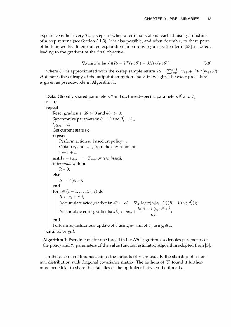
experience either every Tmax steps or when a terminal state is reached, using a mixture
of n-step returns (see Section 3.1.3). It is also possible, and often desirable, to share parts
of both networks. To encourage exploration an entropy regularization term [58] is added,
leading to the gradient of the final objective:
∇θ log π(at|st; θ)(Rt − V π(st; θ)) + βH(π(st; θ)) (3.8)
where Qπ is approximated with the k-step sample return Rt =∑k−1
i=0 γirt+i+γkV π(st+k; θ).
H denotes the entropy of the output distribution and β its weight. The exact procedure
is given as pseudo-code in Algorithm 1.
Data: Globally shared parameters θ and θv; thread-specific parameters θ′
and θ′
v
t = 1;
repeat
Reset gradients: dθ ← 0 and dθv ← 0;
Synchronize parameters: θ′
= θ and θ′
v = θv;
tstart = t;
Get current state st;
repeat
Perform action at based on policy π;
Obtain rt and st+1 from the environment;
t← t+ 1;
until t− tstart == Tmax or terminated;
if terminated then
R = 0;
else
R = V (st; θ);
end
for i ∈ t− 1, . . . , tstart do
R← ri + γR;
Accumulate actor gradients: dθ ← dθ +∇θ′ log π(ai|si; θ
′
)(R− V (si; θ′
v));
Accumulate critic gradients: dθv ← dθv +∂(R− V (si; θ
′
v))2
∂θ′
v
;
end
Perform asynchronous update of θ using dθ and of θv using dθv;
until converged;
Algorithm 1: Pseudo-code for one thread in the A3C algorithm. θ denotes parameters of
the policy and θv parameters of the value function estimator. Algorithm adopted from [5].
In the case of continuous actions the outputs of π are usually the statistics of a nor-
mal distribution with diagonal covariance matrix. The authors of [5] found it further-
more beneficial to share the statistics of the optimizer between the threads.
14 CHAPTER 3. PRELIMINARIES
3.2 Function Approximation with Neural Networks
The classical method to keep track of value functions is to store experienced outcomes
of visited states in a table. This approach has at least two major shortcomings. It does
not allow to generalize between similar states, and it is not directly applicable in continu-
ous state spaces. In scenarios where the table-based setting can not be employed, we can
resort to function approximation techniques instead. The core concept behind function
approximation in RL is to use a statistical model, which is successively adjusted to fit the
value function of the current policy.
There are several options when selecting the model class. Linear function approxima-
tors [59], as the traditional choice, are appealing, because they enjoy theoretical guaran-
tees. However linear models are limited in the set of functions they can represent. Exam-
ples for more flexible models, that have received attention within RL include Gaussian
Processes [60, 61] and neural networks [1, 56].
This thesis focuses on the use of deep networks, which are outlined in the following
subsections. We will start by defining feed-forward and recurrent networks. This is fol-
lowed by explaining the principles behind backpropagation, which is the most common
method for training deep networks. This section is largely based on [62], to which we
refer the reader whenever references are omitted.
3.2.1 Feed-forward Neural Networks
We often find ourselves in the scenario, where we want to determine a function y =
f∗(x), but we do not have any access to f∗ directly. We however can observe correspond-
ing inputs x and outputs y. One approach to solve this problem is to set up a model
f(x; θ), that is parametrized by θ. Once the model is specified, we want to adjust its pa-
rameters θ, such that it becomes the best fit to a given set of samples. Ideally we aim for
models, that generalize well to unseen examples. Feed-forward neural networks are one
class of models, that can be used in such a setting.
Feed-forward neural networks are composed of a set of simple transformations, that
are chained together to obtain the final output. Each of these transformation is referred
to as a layer. Intermediate transformations are called hidden layers. We denote the out-
puts of the lth layer as h(l) and the depth, i.e. the total number of layers, of the network
with L. The standard definition of one layer l is given by:
h(l) = g(l)(W(l)h(l−1) + b(l)) (3.9)
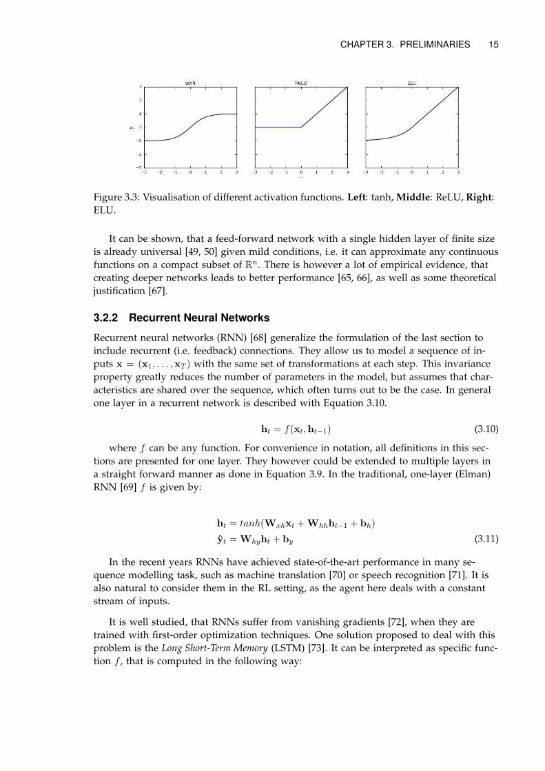
where g(l) is a non-linear activation function. Here common choice include tanh, ReLU
[63] and ELU [64], see Figure 3.3 for a visualisation of their properties. W(l) and b(l) rep-
resent the parameters of a linear transformation. We denote the set of all of these as θ.
h(0) corresponds to the input x and h(L) corresponds to the predicted output y. The out-
put size of the hidden layers can be adjusted and it is commonly selected based on the
difficulty of the task at hand.
The computations of a feed-forward network form a directed acyclic graph, meaning
that no feedback connections are allowed. Extensions to include feedback connections are
presented in the following section.
CHAPTER 3. PRELIMINARIES 15
Figure 3.3: Visualisation of different activation functions. Left: tanh, Middle: ReLU, Right:
ELU.
It can be shown, that a feed-forward network with a single hidden layer of finite size
is already universal [49, 50] given mild conditions, i.e. it can approximate any continuous
functions on a compact subset of Rn. There is however a lot of empirical evidence, that
creating deeper networks leads to better performance [65, 66], as well as some theoretical
justification [67].
3.2.2 Recurrent Neural Networks
Recurrent neural networks (RNN) [68] generalize the formulation of the last section to
include recurrent (i.e. feedback) connections. They allow us to model a sequence of in-
puts x = (x1, . . . ,xT ) with the same set of transformations at each step. This invariance
property greatly reduces the number of parameters in the model, but assumes that char-
acteristics are shared over the sequence, which often turns out to be the case. In general
one layer in a recurrent network is described with Equation 3.10.
ht = f(xt,ht−1) (3.10)
where f can be any function. For convenience in notation, all definitions in this sec-
tions are presented for one layer. They however could be extended to multiple layers in
a straight forward manner as done in Equation 3.9. In the traditional, one-layer (Elman)
RNN [69] f is given by:
ht = tanh(Wxhxt +Whhht−1 + bh)
yt = Whyht + by (3.11)
In the recent years RNNs have achieved state-of-the-art performance in many se-
quence modelling task, such as machine translation [70] or speech recognition [71]. It is
also natural to consider them in the RL setting, as the agent here deals with a constant
stream of inputs.
It is well studied, that RNNs suffer from vanishing gradients [72], when they are
trained with first-order optimization techniques. One solution proposed to deal with this
problem is the Long Short-Term Memory (LSTM) [73]. It can be interpreted as specific func-
tion f , that is computed in the following way:
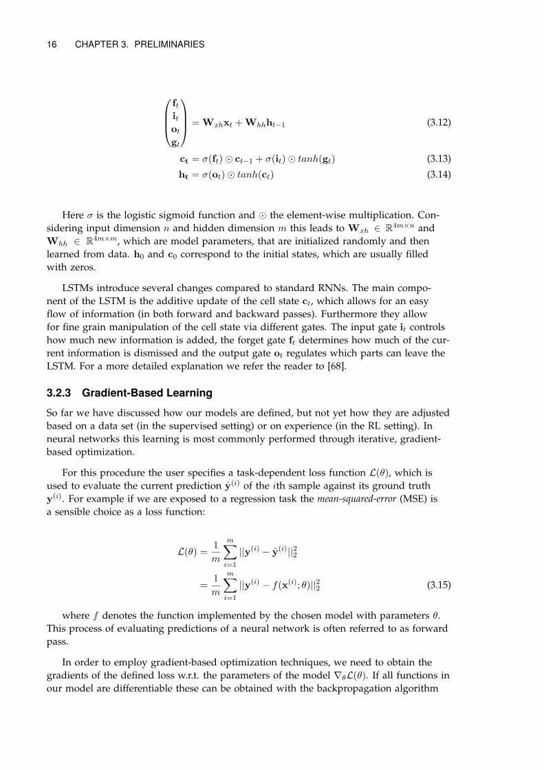
16 CHAPTER 3. PRELIMINARIES
ft
it
ot
gt
= Wxhxt +Whhht−1 (3.12)
ct = σ(ft)⊙ ct−1 + σ(it)⊙ tanh(gt) (3.13)
ht = σ(ot)⊙ tanh(ct) (3.14)
Here σ is the logistic sigmoid function and ⊙ the element-wise multiplication. Con-
sidering input dimension n and hidden dimension m this leads to Wxh ∈ R4m×n and
Whh ∈ R4m×m, which are model parameters, that are initialized randomly and then
learned from data. h0 and c0 correspond to the initial states, which are usually filled
with zeros.
LSTMs introduce several changes compared to standard RNNs. The main compo-
nent of the LSTM is the additive update of the cell state ct, which allows for an easy
flow of information (in both forward and backward passes). Furthermore they allow
for fine grain manipulation of the cell state via different gates. The input gate it controls
how much new information is added, the forget gate ft determines how much of the cur-
rent information is dismissed and the output gate ot regulates which parts can leave the
LSTM. For a more detailed explanation we refer the reader to [68].
3.2.3 Gradient-Based Learning
So far we have discussed how our models are defined, but not yet how they are adjusted
based on a data set (in the supervised setting) or on experience (in the RL setting). In
neural networks this learning is most commonly performed through iterative, gradient-
based optimization.
For this procedure the user specifies a task-dependent loss function L(θ), which is
used to evaluate the current prediction y(i) of the ith sample against its ground truth
y(i). For example if we are exposed to a regression task the mean-squared-error (MSE) is
a sensible choice as a loss function:
L(θ) =1
m
m∑
i=1
||y(i) − y(i)||22
=1
m
m∑
i=1
||y(i) − f(x(i); θ)||22 (3.15)
where f denotes the function implemented by the chosen model with parameters θ.
This process of evaluating predictions of a neural network is often referred to as forward
pass.
In order to employ gradient-based optimization techniques, we need to obtain the
gradients of the defined loss w.r.t. the parameters of the model ∇θL(θ). If all functions in
our model are differentiable these can be obtained with the backpropagation algorithm
CHAPTER 3. PRELIMINARIES 17
f f f f. . .
xt x1 x2 xT
yt y1 y2 yT
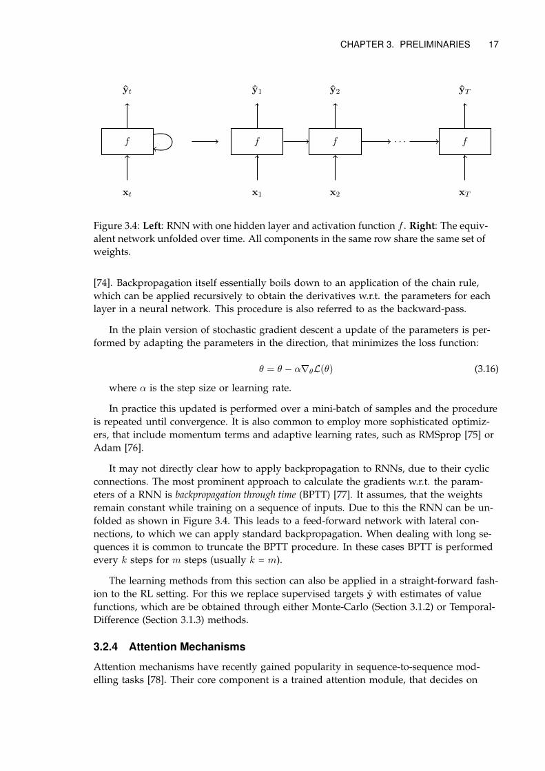
Figure 3.4: Left: RNN with one hidden layer and activation function f . Right: The equiv-
alent network unfolded over time. All components in the same row share the same set of
weights.
[74]. Backpropagation itself essentially boils down to an application of the chain rule,
which can be applied recursively to obtain the derivatives w.r.t. the parameters for each
layer in a neural network. This procedure is also referred to as the backward-pass.
In the plain version of stochastic gradient descent a update of the parameters is per-
formed by adapting the parameters in the direction, that minimizes the loss function:
θ = θ − α∇θL(θ) (3.16)
where α is the step size or learning rate.
In practice this updated is performed over a mini-batch of samples and the procedure
is repeated until convergence. It is also common to employ more sophisticated optimiz-
ers, that include momentum terms and adaptive learning rates, such as RMSprop [75] or
Adam [76].
It may not directly clear how to apply backpropagation to RNNs, due to their cyclic
connections. The most prominent approach to calculate the gradients w.r.t. the param-
eters of a RNN is backpropagation through time (BPTT) [77]. It assumes, that the weights
remain constant while training on a sequence of inputs. Due to this the RNN can be un-
folded as shown in Figure 3.4. This leads to a feed-forward network with lateral con-
nections, to which we can apply standard backpropagation. When dealing with long se-
quences it is common to truncate the BPTT procedure. In these cases BPTT is performed
every k steps for m steps (usually k = m).
The learning methods from this section can also be applied in a straight-forward fash-
ion to the RL setting. For this we replace supervised targets y with estimates of value
functions, which are be obtained through either Monte-Carlo (Section 3.1.2) or Temporal-
Difference (Section 3.1.3) methods.
3.2.4 Attention Mechanisms
Attention mechanisms have recently gained popularity in sequence-to-sequence mod-
elling tasks [78]. Their core component is a trained attention module, that decides on
18 CHAPTER 3. PRELIMINARIES
which part of the representation it wants to focus. In the context of thesis we will em-
ploy an attention mechanism to define suitable goal spaces. Therefore we will briefly re-
view the fundamental concepts in this section.
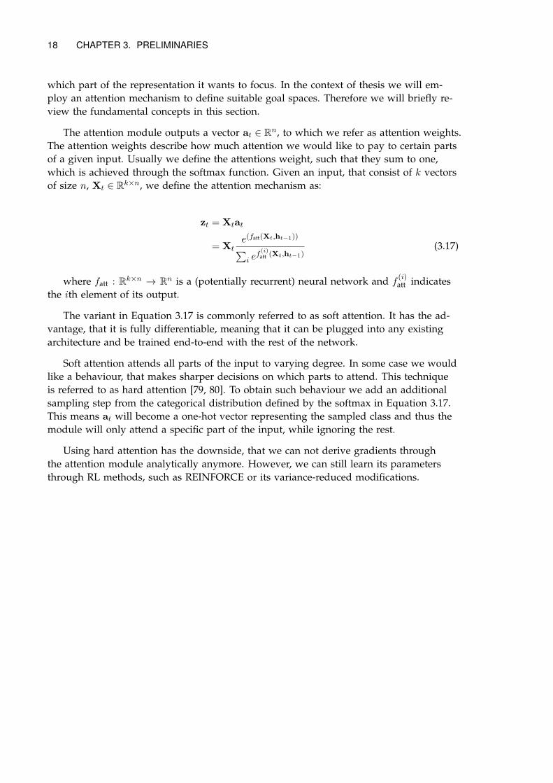
The attention module outputs a vector at ∈ Rn, to which we refer as attention weights.
The attention weights describe how much attention we would like to pay to certain parts
of a given input. Usually we define the attentions weight, such that they sum to one,
which is achieved through the softmax function. Given an input, that consist of k vectors
of size n, Xt ∈ Rk×n, we define the attention mechanism as:
zt = Xtat
= Xte(fatt(Xt,ht−1))
∑
i ef(i)att (Xt,ht−1)
(3.17)
where fatt : Rk×n → R
n is a (potentially recurrent) neural network and f(i)att indicates
the ith element of its output.
The variant in Equation 3.17 is commonly referred to as soft attention. It has the ad-
vantage, that it is fully differentiable, meaning that it can be plugged into any existing
architecture and be trained end-to-end with the rest of the network.
Soft attention attends all parts of the input to varying degree. In some case we would
like a behaviour, that makes sharper decisions on which parts to attend. This technique
is referred to as hard attention [79, 80]. To obtain such behaviour we add an additional
sampling step from the categorical distribution defined by the softmax in Equation 3.17.
This means at will become a one-hot vector representing the sampled class and thus the
module will only attend a specific part of the input, while ignoring the rest.
Using hard attention has the downside, that we can not derive gradients through
the attention module analytically anymore. However, we can still learn its parameters
through RL methods, such as REINFORCE or its variance-reduced modifications.
CHAPTER 3. PRELIMINARIES 19
3.3 Hierarchical Reinforcement Learning
Hierarchical Reinforcement Learning describes a set of methods, that attempt to extend
standard RL agents with some form of hierarchical structure. We have already mentioned
some of these techniques in Chapter 2.
Learning good temporal abstractions is one of the key challenges in RL. It does not
only allow to decompose the task in sub-components, that are easier to solve, but also
enables to reuse already learned solutions, potentially speeding up the training process
by orders of magnitude.
In this section we will review the options [25] framework, which is a popular choices
for incorporating temporal abstractions in existing RL methods. Furthermore we outline
Universal Value Function Approximators (UVFA) [30], which allow to transfer knowledge
between different options. Together these techniques form the core of the approach pro-
posed in the following chapter.
3.3.1 Options Framework
Options [25] extend the agent’s available behaviour through a set of temporally extended
actions. Instead of choosing a primitive action, the agents is allowed to select an option
from a set Ω, which is then followed until a termination criterion is met. Examples for
options include grasping an object, opening a door and also the agent’s primitive actions.
Mathematically an option ω is defined as a triple (Iω, πω, βω), where Iω ⊆ S is the
initiation set, βω : S → [0, 1] the termination condition and πω : S → A the intra-option
policy. For simplicity it is often assumed, that all options are available everywhere, i.e.
Iω = S for all ω.
A set of options defined over a MDP constitutes a semi-MDP [25]. As the theory of
semi-MDPs is closely related to that of MDPs, we can carry other many theoretical guar-
antees when dealing with options. The framework itself does however not define, how
suitable options arise. We have already reviewed several extensions, that strive to dis-
cover options from experience, in Chapter 2.
It is intuitive to think of options as a procedure for archiving a sub-goal, but it may
also be not immediately clear how such a behaviour emerges. Given, that we know the
set of suitable sub-goals, we can assign an option to each these, along with an intrinsic
reward function. The intrinsic reward should assign high values for archiving the sub-
goal and low values otherwise. If we now learn the intra-option policies based on the
intrinsic reward functions we already obtain a type of goal-directed behaviour.
3.3.2 Universal Value Function Approximators
The interpretation of options as sub-goals provided in the last paragraph, would require
to learn separate values functions Vg(s) for each possible sub-goal g. Learning many, in-
dependent values functions can be slow and does not scale well to settings with a large
number of possible sub-goals.
To circumvent these issues Universal Value Function Approximators (UVFA) [30]

20 CHAPTER 3. PRELIMINARIES
approximate the union of value functions for all goals with V (s,g; θ). In practice this
means, that the goal is provide as part of the input to the value function approximator.
In the simplest case this is realized through concatenation of state and goal. UVFAs are
able to exploit additional structure in the goal space and thus enable faster learning and
better generalization. Furthermore they scale easily to large or even uncountable sets of
goals.
Chapter 4
Methods
4.1 Hierarchical Reinforcement Learning with Goals
In this section we extend the RL framework to include an explicit goal-directed mecha-
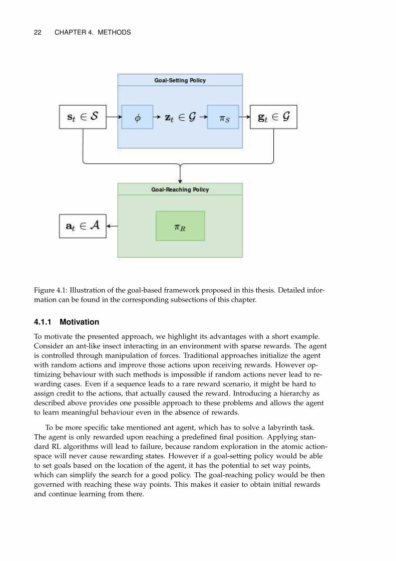
nism. For this the agent’s internals are separated in two parts – a goal-setting policy πS ,
which is responsible to set goals and a goal-reaching policy πR, which has to reach the
goals given by the goal-setting policy1. An illustration describing the concept is given in
Figure 4.1. The model is constructed in a way, that both parts can be learned simultane-
ously through arbitrary RL methods. We will however argue later in this chapter, that
certain choices are more sensible than others. Note, that similar architecture have been
applied in prior work [21, 22, 81]. The relation to these methods will be further discussed
in Section 4.2.
The goal-setting agents operates on some continuous goal space G ⊆ Rk. In the most
general case it learns a function φ : S → Rk, that maps from the current state st to the
current activation in goal space zt. We will also refer to φ(st) as goal embedding in the
following. In the initial state and whenever the current goal was reached a new goal
is selected. We interpret setting goals as actions of the goal-setting policy represented
through πS : G → Rk. This allows to apply standard RL techniques for the goal-setting
policy. The goal-setting agent’s actions last over multiple time steps and its rewards are
defined as the sum of external rewards from the environment along the path towards the
goal. The goal-reaching policy πR on the other hand acts through the agent’s atomic ac-
tions at each time-step and gets rewarded for reaching the goal set from the goal-setting
policy. The complete method is outlined in Algorithm 2.
In the following we will first highlight possible advantages compared to standard RL
approaches, explained on an idealized example. We describe specific design choices – for
both goal-setting and goal-reaching policies – used during the experiments in this report.
We then provide a connection to the options framework, which provides some theoretical
grounding for the approach. Finally we highlight connections and differences to related
approaches.
1Other works also refer to these two policies as high- and low-level policy or as manager and worker.
21
22 CHAPTER 4. METHODS
Figure 4.1: Illustration of the goal-based framework proposed in this thesis. Detailed infor-
mation can be found in the corresponding subsections of this chapter.
4.1.1 Motivation
To motivate the presented approach, we highlight its advantages with a short example.
Consider an ant-like insect interacting in an environment with sparse rewards. The agent
is controlled through manipulation of forces. Traditional approaches initialize the agent
with random actions and improve those actions upon receiving rewards. However op-
timizing behaviour with such methods is impossible if random actions never lead to re-
warding cases. Even if a sequence leads to a rare reward scenario, it might be hard to
assign credit to the actions, that actually caused the reward. Introducing a hierarchy as
described above provides one possible approach to these problems and allows the agent
to learn meaningful behaviour even in the absence of rewards.
To be more specific take mentioned ant agent, which has to solve a labyrinth task.
The agent is only rewarded upon reaching a predefined final position. Applying stan-
dard RL algorithms will lead to failure, because random exploration in the atomic action-
space will never cause rewarding states. However if a goal-setting policy would be able
to set goals based on the location of the agent, it has the potential to set way points,
which can simplify the search for a good policy. The goal-reaching policy would be then
governed with reaching these way points. This makes it easier to obtain initial rewards
and continue learning from there.
CHAPTER 4. METHODS 23
Ideally we learn the desired goal space from experience, however in some domains
we can also consider the simpler case of using pre-designed embeddings and only learn
transitions in the given space. Learning goal embedding greatly increases the generality
of the procedure, at the cost of introducing additional complexity. We will investigate
both cases during later sections in this report.
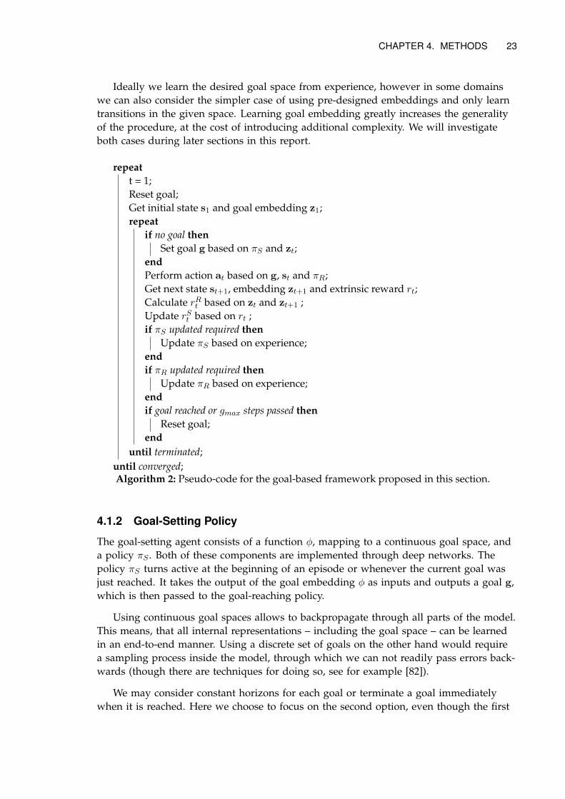
repeat
t = 1;
Reset goal;
Get initial state s1 and goal embedding z1;
repeat
if no goal then
Set goal g based on πS and zt;
end
Perform action at based on g, st and πR;
Get next state st+1, embedding zt+1 and extrinsic reward rt;
Calculate rRt based on zt and zt+1 ;
Update rSt based on rt ;
if πS updated required then
Update πS based on experience;
end
if πR updated required then
Update πR based on experience;
end
if goal reached or gmax steps passed then
Reset goal;
end
until terminated;
until converged;Algorithm 2: Pseudo-code for the goal-based framework proposed in this section.
4.1.2 Goal-Setting Policy
The goal-setting agent consists of a function φ, mapping to a continuous goal space, and
a policy πS . Both of these components are implemented through deep networks. The
policy πS turns active at the beginning of an episode or whenever the current goal was
just reached. It takes the output of the goal embedding φ as inputs and outputs a goal g,
which is then passed to the goal-reaching policy.
Using continuous goal spaces allows to backpropagate through all parts of the model.
This means, that all internal representations – including the goal space – can be learned
in an end-to-end manner. Using a discrete set of goals on the other hand would require
a sampling process inside the model, through which we can not readily pass errors back-
wards (though there are techniques for doing so, see for example [82]).
We may consider constant horizons for each goal or terminate a goal immediately
when it is reached. Here we choose to focus on the second option, even though the first
24 CHAPTER 4. METHODS
one might have its own advantages. We denote the maximum time-span a goal is active
in the following as gmax. The reward of the goal-setting policy is based in the extrinsic
reward of the environment along the taken path towards the goal, defined as:
rSt =k
∑
n=1
rt+n (4.1)
where k is bounded from above through gmax.
We now have defined all components of the goal-setting MDP, that are required to
learn about its policy. This means we can directly apply any RL algorithm to this prob-
lem. Here we decide to employ A3C (Section 3.1.5) as the method of choice.
It is worth mentioning, that the state-transition distribution of the goal-setting MDP
pS is dependent on the behaviour of the goal-reaching policy. This means, that there
might be cases in which goals are not reached. In order to encourage learning, based on
transition of the goal-reaching policy, we propose a modified version of the update rule
from Equation 3.8:
∇θS log πS(zt+k|st; θS)(Rt − V πS (st; θS)) (4.2)
where gt is replaced with the reached location in goal space zt+k.
The goal-setting policy is, by definition, exposed to less data then the goal-reaching
policy, as it operates at a slower time-scale. This could make learning challenging. We
will later discuss methods, that could enable more data-efficient learning.
4.1.3 Goal-Reaching Policy
The goal-reaching policy πR is, in contrast to the goal-setting policy, active at every time-
step and responsible for selecting the agents primitive actions. Let n be the nth step, af-
ter a new goal was set at time-step t. At each time-step t + n the agent receives infor-
mation about the currently active goal (for example as relative or absolute values). In
practice we just pass this information as an additional input to the policy and value net-
works. This process is a form of UVFA, as described in Section 3.3.2, where the set of
possible goals is a continuous vector space. Therefore the agent is able to generalize be-
tween all possible goals.
The goal-reaching polices in this report will learned with the A3C algorithm as de-
scribed in Section 3.1.5, where policies are represented through deep networks. Network
architectures will be described in more detail during the later parts of this report. The
goal-reaching policy adapts its behaviour to maximize an intrinsic reward rRt+n, which is
based on some distance measure d between the current position in goal space zt+n and
the active goal gt:
rRt+n = −d(zt+n,gt) (4.3)
where the choice of d can be adapted to the given scenario. In practice we can also
combine this reward with the extrinsic reward rt+n from the environment. A similar
technique, based on a linear combination of both terms, was shown to be beneficial in
[22]. Here we will simply add all control-based rewards (if available) from rt+n to rRt+n.
CHAPTER 4. METHODS 25
Name Domain Actions Goals Learning UVFA
HASSLE [23] Navigation discrete ARAVQ Advantage
Learning
Horde [39] Mobile Robots discrete Demons GQ(λ)
h-DQN [21] ATARI discrete Entities & Relations DQN
FuN [22] ATARI discrete Learned A3C*
DeepLab
DeepLoco [24] Bullet continuous Footsteps Actor-Critic
ours MuJoCo continuous Learned A3C
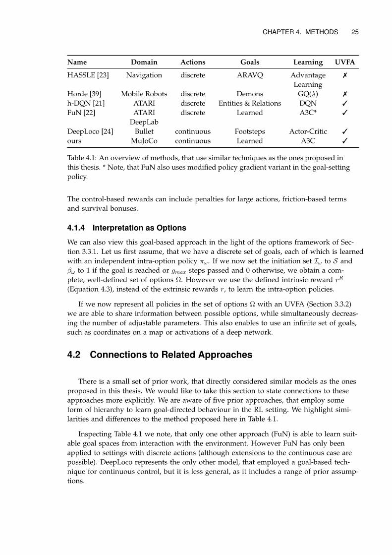
Table 4.1: An overview of methods, that use similar techniques as the ones proposed in
this thesis. * Note, that FuN also uses modified policy gradient variant in the goal-setting
policy.
The control-based rewards can include penalties for large actions, friction-based terms
and survival bonuses.
4.1.4 Interpretation as Options
We can also view this goal-based approach in the light of the options framework of Sec-
tion 3.3.1. Let us first assume, that we have a discrete set of goals, each of which is learned
with an independent intra-option policy πω. If we now set the initiation set Iω to S and
βω to 1 if the goal is reached or gmax steps passed and 0 otherwise, we obtain a com-
plete, well-defined set of options Ω. However we use the defined intrinsic reward rR
(Equation 4.3), instead of the extrinsic rewards r, to learn the intra-option policies.
If we now represent all policies in the set of options Ω with an UVFA (Section 3.3.2)
we are able to share information between possible options, while simultaneously decreas-
ing the number of adjustable parameters. This also enables to use an infinite set of goals,
such as coordinates on a map or activations of a deep network.
4.2 Connections to Related Approaches
There is a small set of prior work, that directly considered similar models as the ones
proposed in this thesis. We would like to take this section to state connections to these
approaches more explicitly. We are aware of five prior approaches, that employ some
form of hierarchy to learn goal-directed behaviour in the RL setting. We highlight simi-
larities and differences to the method proposed here in Table 4.1.
Inspecting Table 4.1 we note, that only one other approach (FuN) is able to learn suit-
able goal spaces from interaction with the environment. However FuN has only been
applied to settings with discrete actions (although extensions to the continuous case are
possible). DeepLoco represents the only other model, that employed a goal-based tech-
nique for continuous control, but it is less general, as it includes a range of prior assump-
tions.
Chapter 5
Experiments
Next we will examine the methods proposed in the last chapter on a set of continuous
control problems of increasing difficulty. For this we will consider a simple point-mass
model and several challenging tasks based on the MuJoCo physics simulator [18]. More
specifically we aim to control the following agents:
• Point-Mass: Here we control the acceleration of a simple point-mass model. The
4 dimensional observation space consists of the current position and velocity. We
restrict both the acceleration and velocity to be within a fixed range.
• Half-Cheetah [83]: A planar biped robot with 9 rigid links. Its 20 dimensional ob-
servation space includes information about the center of mass, joint angles and joint
velocities. It is controlled through the manipulation of 6 actuated joints.
• Ant [16]: A ant-like insect with 13 rigid links. The 125 dimensional observation
space contains the center of mass joint angles, joint velocities, a (usually sparse)
vector of contact forces and the rotation matrix for the body. Control is performed
via 8 actuated joints. Further it is possible for the robot to die, i.e. to fall over and
get into a configuration from which it can not recover.
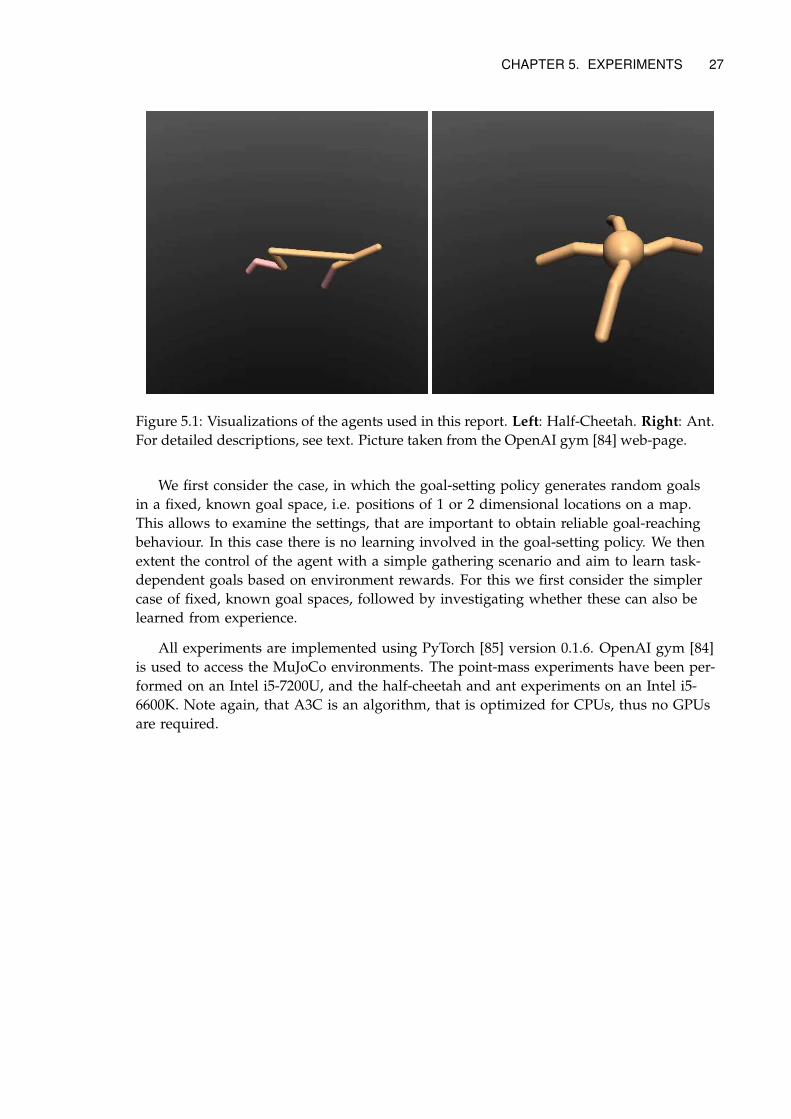
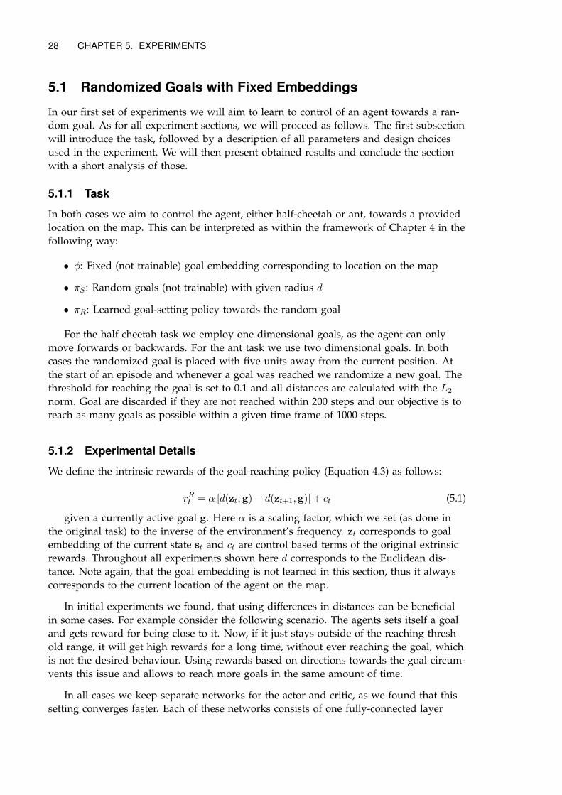
The latter two of these descriptions have been partially adopted from [19]. Figure 5.1
includes visualizations of the described agents. These tasks are appealing, because con-
trolling the agent’s actions is challenging even if we only consider the simple scenario of
moving in one direction, as it is done in common benchmarks [19]. Yet it is easy to in-
corporate these agents into scenarios with sparse rewards, such as navigation through
a labyrinth or gathering objects. Employing such a setup allows to stretch the capabili-
ties of both goal-setting and goal-reaching polices. On the other hand we can often rea-
son about the structure of a suitable goal space and thus incorporate prior knowledge
into the problem. This comes in handy because it allows to first attempt the easier task,
where the goal space is known, and then continue to cases where it is learned end-to-
end. Additionally we have included the point-mass model, as it is allows for a faster
evaluation of the given methods.
The experiments in this section are structured based on the three components of goal-
directed behaviour outlined in Chapters 1 and 4. We aim to build an incremental solu-
tion to the full problem, starting with easier settings.
26
CHAPTER 5. EXPERIMENTS 27
Figure 5.1: Visualizations of the agents used in this report. Left: Half-Cheetah. Right: Ant.
For detailed descriptions, see text. Picture taken from the OpenAI gym [84] web-page.
We first consider the case, in which the goal-setting policy generates random goals
in a fixed, known goal space, i.e. positions of 1 or 2 dimensional locations on a map.
This allows to examine the settings, that are important to obtain reliable goal-reaching
behaviour. In this case there is no learning involved in the goal-setting policy. We then
extent the control of the agent with a simple gathering scenario and aim to learn task-
dependent goals based on environment rewards. For this we first consider the simpler
case of fixed, known goal spaces, followed by investigating whether these can also be
learned from experience.
All experiments are implemented using PyTorch [85] version 0.1.6. OpenAI gym [84]
is used to access the MuJoCo environments. The point-mass experiments have been per-
formed on an Intel i5-7200U, and the half-cheetah and ant experiments on an Intel i5-
6600K. Note again, that A3C is an algorithm, that is optimized for CPUs, thus no GPUs
are required.
28 CHAPTER 5. EXPERIMENTS
5.1 Randomized Goals with Fixed Embeddings
In our first set of experiments we will aim to learn to control of an agent towards a ran-
dom goal. As for all experiment sections, we will proceed as follows. The first subsection
will introduce the task, followed by a description of all parameters and design choices
used in the experiment. We will then present obtained results and conclude the section
with a short analysis of those.
5.1.1 Task
In both cases we aim to control the agent, either half-cheetah or ant, towards a provided
location on the map. This can be interpreted as within the framework of Chapter 4 in the
following way:
• φ: Fixed (not trainable) goal embedding corresponding to location on the map
• πS : Random goals (not trainable) with given radius d
• πR: Learned goal-setting policy towards the random goal
For the half-cheetah task we employ one dimensional goals, as the agent can only
move forwards or backwards. For the ant task we use two dimensional goals. In both
cases the randomized goal is placed with five units away from the current position. At
the start of an episode and whenever a goal was reached we randomize a new goal. The
threshold for reaching the goal is set to 0.1 and all distances are calculated with the L2
norm. Goal are discarded if they are not reached within 200 steps and our objective is to
reach as many goals as possible within a given time frame of 1000 steps.
5.1.2 Experimental Details
We define the intrinsic rewards of the goal-reaching policy (Equation 4.3) as follows:
rRt = α [d(zt,g)− d(zt+1,g)] + ct (5.1)
given a currently active goal g. Here α is a scaling factor, which we set (as done in
the original task) to the inverse of the environment’s frequency. zt corresponds to goal
embedding of the current state st and ct are control based terms of the original extrinsic
rewards. Throughout all experiments shown here d corresponds to the Euclidean dis-
tance. Note again, that the goal embedding is not learned in this section, thus it always
corresponds to the current location of the agent on the map.
In initial experiments we found, that using differences in distances can be beneficial
in some cases. For example consider the following scenario. The agents sets itself a goal
and gets reward for being close to it. Now, if it just stays outside of the reaching thresh-
old range, it will get high rewards for a long time, without ever reaching the goal, which
is not the desired behaviour. Using rewards based on directions towards the goal circum-
vents this issue and allows to reach more goals in the same amount of time.
In all cases we keep separate networks for the actor and critic, as we found that this
setting converges faster. Each of these networks consists of one fully-connected layer
CHAPTER 5. EXPERIMENTS 29
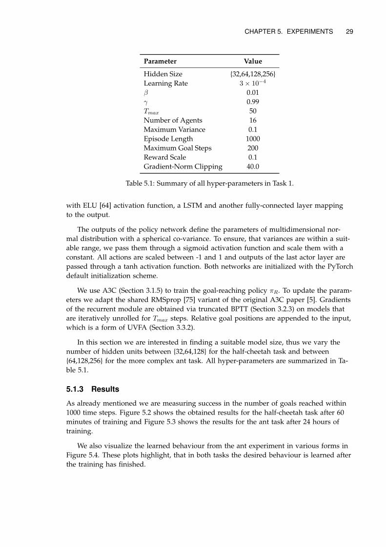
Parameter Value
Hidden Size 32,64,128,256
Learning Rate 3× 10⁻⁴
β 0.01
γ 0.99
Tmax 50
Number of Agents 16
Maximum Variance 0.1
Episode Length 1000
Maximum Goal Steps 200
Reward Scale 0.1
Gradient-Norm Clipping 40.0
Table 5.1: Summary of all hyper-parameters in Task 1.
with ELU [64] activation function, a LSTM and another fully-connected layer mapping
to the output.
The outputs of the policy network define the parameters of multidimensional nor-
mal distribution with a spherical co-variance. To ensure, that variances are within a suit-
able range, we pass them through a sigmoid activation function and scale them with a
constant. All actions are scaled between -1 and 1 and outputs of the last actor layer are
passed through a tanh activation function. Both networks are initialized with the PyTorch
default initialization scheme.
We use A3C (Section 3.1.5) to train the goal-reaching policy πR. To update the param-
eters we adapt the shared RMSprop [75] variant of the original A3C paper [5]. Gradients
of the recurrent module are obtained via truncated BPTT (Section 3.2.3) on models that
are iteratively unrolled for Tmax steps. Relative goal positions are appended to the input,
which is a form of UVFA (Section 3.3.2).
In this section we are interested in finding a suitable model size, thus we vary the
number of hidden units between 32,64,128 for the half-cheetah task and between
64,128,256 for the more complex ant task. All hyper-parameters are summarized in Ta-
ble 5.1.
5.1.3 Results
As already mentioned we are measuring success in the number of goals reached within
1000 time steps. Figure 5.2 shows the obtained results for the half-cheetah task after 60
minutes of training and Figure 5.3 shows the results for the ant task after 24 hours of
training.
We also visualize the learned behaviour from the ant experiment in various forms in
Figure 5.4. These plots highlight, that in both tasks the desired behaviour is learned after
the training has finished.
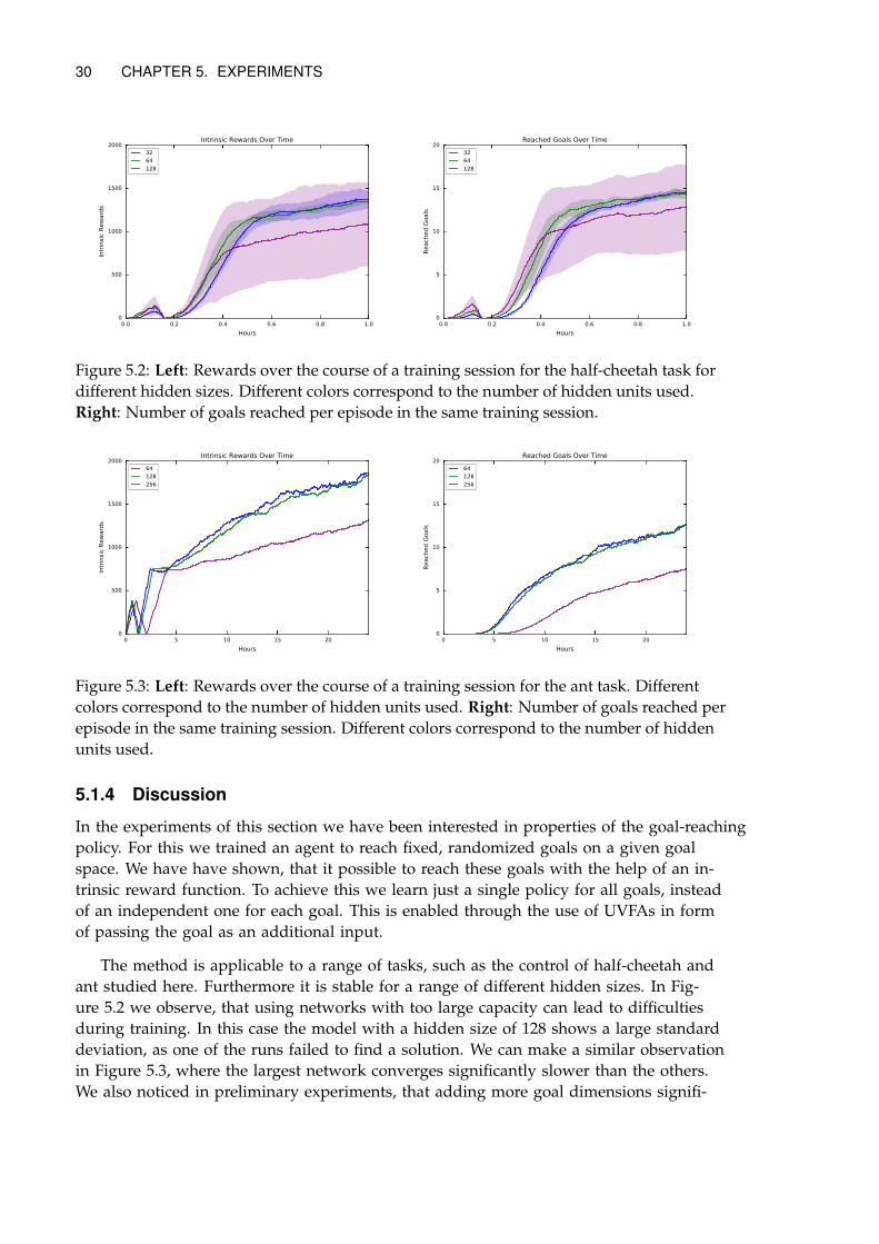
30 CHAPTER 5. EXPERIMENTS
0.0 0.2 0.4 0.6 0.8 1.0
Hours
0
500
1000
1500
2000
Intr
insi
c R
ew
ard
s
Intrinsic Rewards Over Time
32
64
128
0.0 0.2 0.4 0.6 0.8 1.0
Hours
0
5
10
15
20
Reach
ed G
oals
Reached Goals Over Time
32
64
128
Figure 5.2: Left: Rewards over the course of a training session for the half-cheetah task for
different hidden sizes. Different colors correspond to the number of hidden units used.
Right: Number of goals reached per episode in the same training session.
0 5 10 15 20
Hours
0
500
1000
1500
2000
Intr
insi
c R
ew
ard
s
Intrinsic Rewards Over Time
64
128
256
0 5 10 15 20
Hours
0
5
10
15
20
Reach
ed G
oals
Reached Goals Over Time
64
128
256
Figure 5.3: Left: Rewards over the course of a training session for the ant task. Different
colors correspond to the number of hidden units used. Right: Number of goals reached per
episode in the same training session. Different colors correspond to the number of hidden
units used.
5.1.4 Discussion
In the experiments of this section we have been interested in properties of the goal-reaching
policy. For this we trained an agent to reach fixed, randomized goals on a given goal
space. We have have shown, that it possible to reach these goals with the help of an in-
trinsic reward function. To achieve this we learn just a single policy for all goals, instead
of an independent one for each goal. This is enabled through the use of UVFAs in form
of passing the goal as an additional input.
The method is applicable to a range of tasks, such as the control of half-cheetah and
ant studied here. Furthermore it is stable for a range of different hidden sizes. In Fig-
ure 5.2 we observe, that using networks with too large capacity can lead to difficulties
during training. In this case the model with a hidden size of 128 shows a large standard
deviation, as one of the runs failed to find a solution. We can make a similar observation
in Figure 5.3, where the largest network converges significantly slower than the others.
We also noticed in preliminary experiments, that adding more goal dimensions signifi-
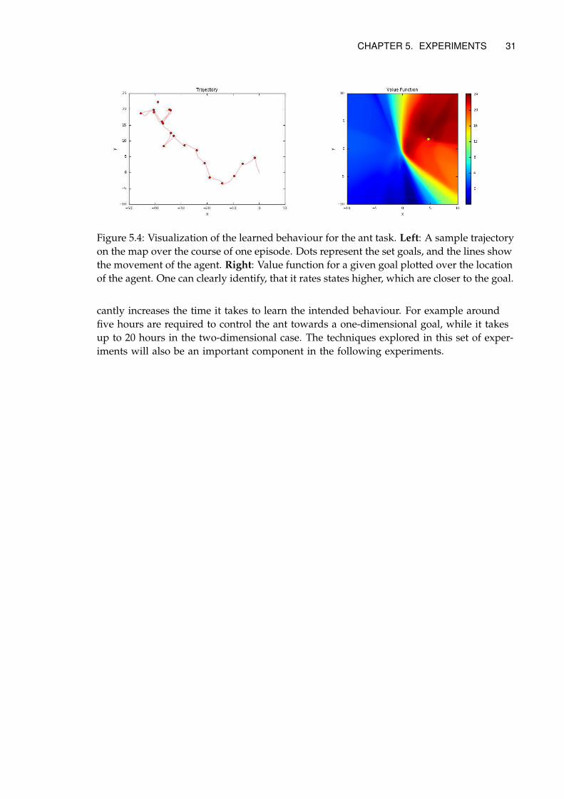
CHAPTER 5. EXPERIMENTS 31
Figure 5.4: Visualization of the learned behaviour for the ant task. Left: A sample trajectory
on the map over the course of one episode. Dots represent the set goals, and the lines show
the movement of the agent. Right: Value function for a given goal plotted over the location
of the agent. One can clearly identify, that it rates states higher, which are closer to the goal.
cantly increases the time it takes to learn the intended behaviour. For example around
five hours are required to control the ant towards a one-dimensional goal, while it takes
up to 20 hours in the two-dimensional case. The techniques explored in this set of exper-
iments will also be an important component in the following experiments.
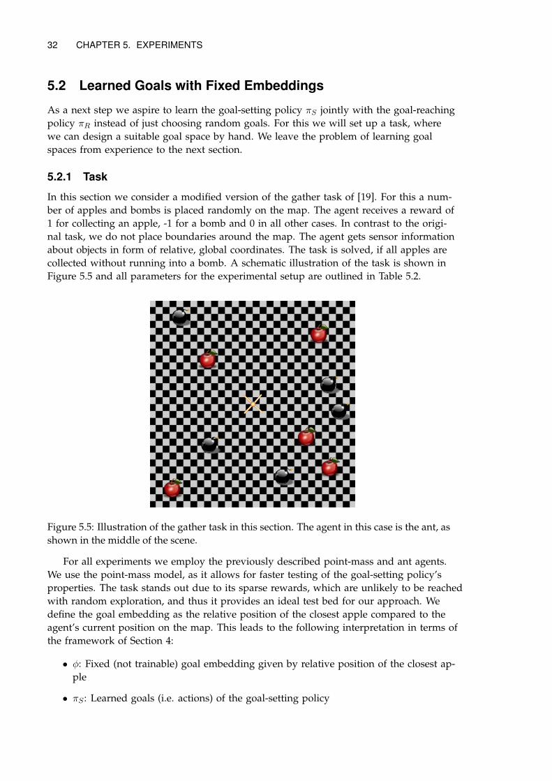
32 CHAPTER 5. EXPERIMENTS
5.2 Learned Goals with Fixed Embeddings
As a next step we aspire to learn the goal-setting policy πS jointly with the goal-reaching
policy πR instead of just choosing random goals. For this we will set up a task, where
we can design a suitable goal space by hand. We leave the problem of learning goal
spaces from experience to the next section.
5.2.1 Task
In this section we consider a modified version of the gather task of [19]. For this a num-
ber of apples and bombs is placed randomly on the map. The agent receives a reward of
1 for collecting an apple, -1 for a bomb and 0 in all other cases. In contrast to the origi-
nal task, we do not place boundaries around the map. The agent gets sensor information
about objects in form of relative, global coordinates. The task is solved, if all apples are
collected without running into a bomb. A schematic illustration of the task is shown in
Figure 5.5 and all parameters for the experimental setup are outlined in Table 5.2.
Figure 5.5: Illustration of the gather task in this section. The agent in this case is the ant, as
shown in the middle of the scene.
For all experiments we employ the previously described point-mass and ant agents.
We use the point-mass model, as it allows for faster testing of the goal-setting policy’s
properties. The task stands out due to its sparse rewards, which are unlikely to be reached
with random exploration, and thus it provides an ideal test bed for our approach. We
define the goal embedding as the relative position of the closest apple compared to the
agent’s current position on the map. This leads to the following interpretation in terms of
the framework of Section 4:
• φ: Fixed (not trainable) goal embedding given by relative position of the closest ap-
ple
• πS : Learned goals (i.e. actions) of the goal-setting policy
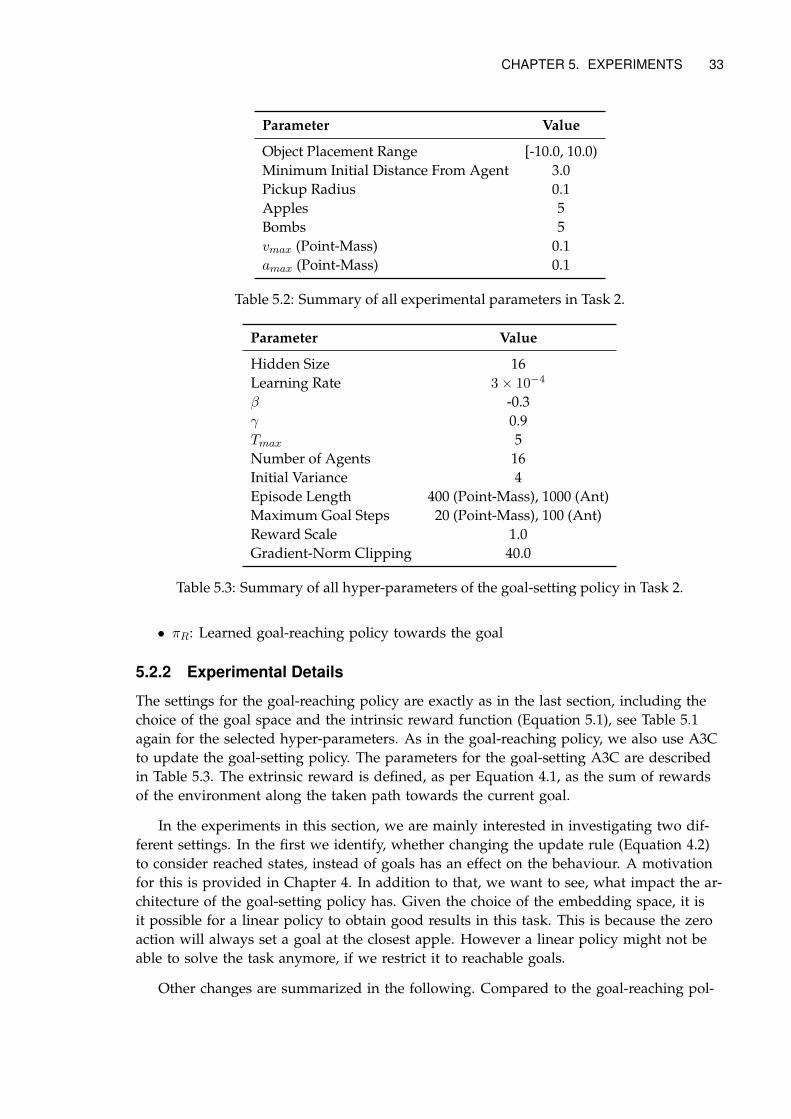
CHAPTER 5. EXPERIMENTS 33
Parameter Value
Object Placement Range [-10.0, 10.0)
Minimum Initial Distance From Agent 3.0
Pickup Radius 0.1
Apples 5
Bombs 5
vmax (Point-Mass) 0.1
amax (Point-Mass) 0.1
Table 5.2: Summary of all experimental parameters in Task 2.
Parameter Value
Hidden Size 16
Learning Rate 3× 10⁻⁴
β -0.3
γ 0.9
Tmax 5
Number of Agents 16
Initial Variance 4
Episode Length 400 (Point-Mass), 1000 (Ant)
Maximum Goal Steps 20 (Point-Mass), 100 (Ant)
Reward Scale 1.0
Gradient-Norm Clipping 40.0
Table 5.3: Summary of all hyper-parameters of the goal-setting policy in Task 2.
• πR: Learned goal-reaching policy towards the goal
5.2.2 Experimental Details
The settings for the goal-reaching policy are exactly as in the last section, including the
choice of the goal space and the intrinsic reward function (Equation 5.1), see Table 5.1
again for the selected hyper-parameters. As in the goal-reaching policy, we also use A3C
to update the goal-setting policy. The parameters for the goal-setting A3C are described
in Table 5.3. The extrinsic reward is defined, as per Equation 4.1, as the sum of rewards
of the environment along the taken path towards the current goal.
In the experiments in this section, we are mainly interested in investigating two dif-
ferent settings. In the first we identify, whether changing the update rule (Equation 4.2)
to consider reached states, instead of goals has an effect on the behaviour. A motivation
for this is provided in Chapter 4. In addition to that, we want to see, what impact the ar-
chitecture of the goal-setting policy has. Given the choice of the embedding space, it is
it possible for a linear policy to obtain good results in this task. This is because the zero
action will always set a goal at the closest apple. However a linear policy might not be
able to solve the task anymore, if we restrict it to reachable goals.
Other changes are summarized in the following. Compared to the goal-reaching pol-
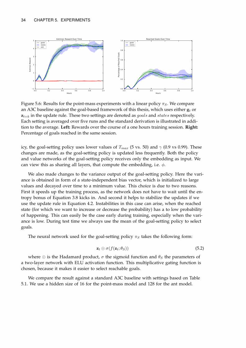
34 CHAPTER 5. EXPERIMENTS
0.0 0.2 0.4 0.6 0.8 1.0
Hours
1
0
1
2
3
4
5
Extr
insi
c R
ew
ard
Extrinsic Reward Over Time
goals
states
A3C
0.0 0.2 0.4 0.6 0.8 1.0
Hours
0.0
0.2
0.4
0.6
0.8
1.0
Perc
enta
ge o
f R
each
ed G
oals
Reached Goals Over Time
goals
states
Figure 5.6: Results for the point-mass experiments with a linear policy πS . We compare
an A3C baseline against the goal-based framework of this thesis, which uses either gt or
zt+k in the update rule. These two settings are denoted as goals and states respectively.
Each setting is averaged over five runs and the standard derivation is illustrated in addi-
tion to the average. Left: Rewards over the course of a one hours training session. Right:
Percentage of goals reached in the same session.
icy, the goal-setting policy uses lower values of Tmax (5 vs. 50) and γ (0.9 vs 0.99). These
changes are made, as the goal-setting policy is updated less frequently. Both the policy
and value networks of the goal-setting policy receives only the embedding as input. We
can view this as sharing all layers, that compute the embedding, i.e. φ.
We also made changes to the variance output of the goal-setting policy. Here the vari-
ance is obtained in form of a state-independent bias vector, which is initialized to large
values and decayed over time to a minimum value. This choice is due to two reasons.
First it speeds up the training process, as the network does not have to wait until the en-
tropy bonus of Equation 3.8 kicks in. And second it helps to stabilize the updates if we
use the update rule in Equation 4.2. Instabilities in this case can arise, when the reached
state (for which we want to increase or decrease the probability) has a to low probability
of happening. This can easily be the case early during training, especially when the vari-
ance is low. During test time we always use the mean of the goal-setting policy to select
goals.
The neural network used for the goal-setting policy πS takes the following form:
zt ⊙ σ(f(zt; θS)) (5.2)
where ⊙ is the Hadamard product, σ the sigmoid function and θS the parameters of
a two-layer network with ELU activation function. This multiplicative gating function is
chosen, because it makes it easier to select reachable goals.
We compare the result against a standard A3C baseline with settings based on Table
5.1. We use a hidden size of 16 for the point-mass model and 128 for the ant model.
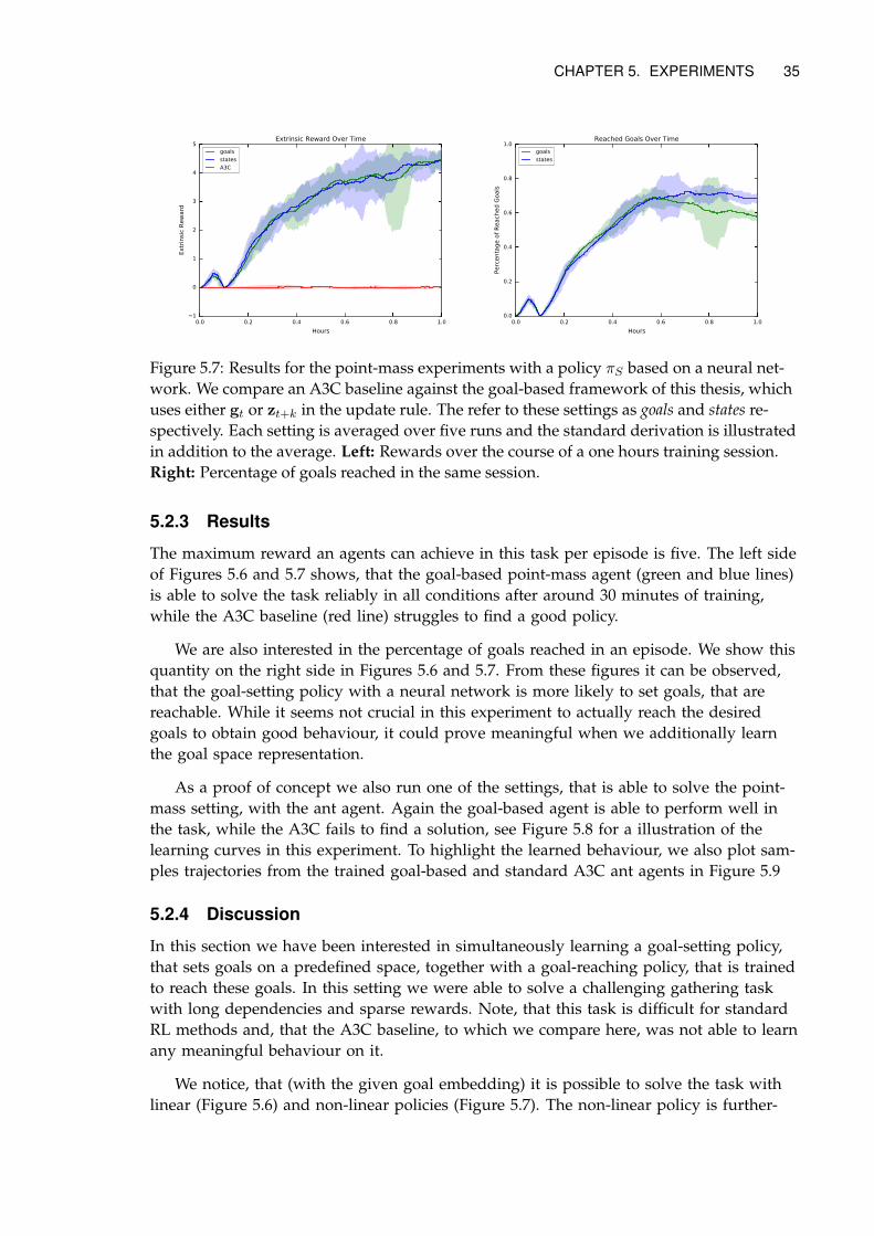
CHAPTER 5. EXPERIMENTS 35
0.0 0.2 0.4 0.6 0.8 1.0
Hours
1
0
1
2
3
4
5
Extr
insi
c R
ew
ard
Extrinsic Reward Over Time
goals
states
A3C
0.0 0.2 0.4 0.6 0.8 1.0
Hours
0.0
0.2
0.4
0.6
0.8
1.0
Perc
enta
ge o
f R
each
ed G
oals
Reached Goals Over Time
goals
states
Figure 5.7: Results for the point-mass experiments with a policy πS based on a neural net-
work. We compare an A3C baseline against the goal-based framework of this thesis, which
uses either gt or zt+k in the update rule. The refer to these settings as goals and states re-
spectively. Each setting is averaged over five runs and the standard derivation is illustrated
in addition to the average. Left: Rewards over the course of a one hours training session.
Right: Percentage of goals reached in the same session.
5.2.3 Results
The maximum reward an agents can achieve in this task per episode is five. The left side
of Figures 5.6 and 5.7 shows, that the goal-based point-mass agent (green and blue lines)
is able to solve the task reliably in all conditions after around 30 minutes of training,
while the A3C baseline (red line) struggles to find a good policy.
We are also interested in the percentage of goals reached in an episode. We show this
quantity on the right side in Figures 5.6 and 5.7. From these figures it can be observed,
that the goal-setting policy with a neural network is more likely to set goals, that are
reachable. While it seems not crucial in this experiment to actually reach the desired
goals to obtain good behaviour, it could prove meaningful when we additionally learn
the goal space representation.
As a proof of concept we also run one of the settings, that is able to solve the point-
mass setting, with the ant agent. Again the goal-based agent is able to perform well in
the task, while the A3C fails to find a solution, see Figure 5.8 for a illustration of the
learning curves in this experiment. To highlight the learned behaviour, we also plot sam-
ples trajectories from the trained goal-based and standard A3C ant agents in Figure 5.9
5.2.4 Discussion
In this section we have been interested in simultaneously learning a goal-setting policy,
that sets goals on a predefined space, together with a goal-reaching policy, that is trained
to reach these goals. In this setting we were able to solve a challenging gathering task
with long dependencies and sparse rewards. Note, that this task is difficult for standard
RL methods and, that the A3C baseline, to which we compare here, was not able to learn
any meaningful behaviour on it.
We notice, that (with the given goal embedding) it is possible to solve the task with
linear (Figure 5.6) and non-linear policies (Figure 5.7). The non-linear policy is further-
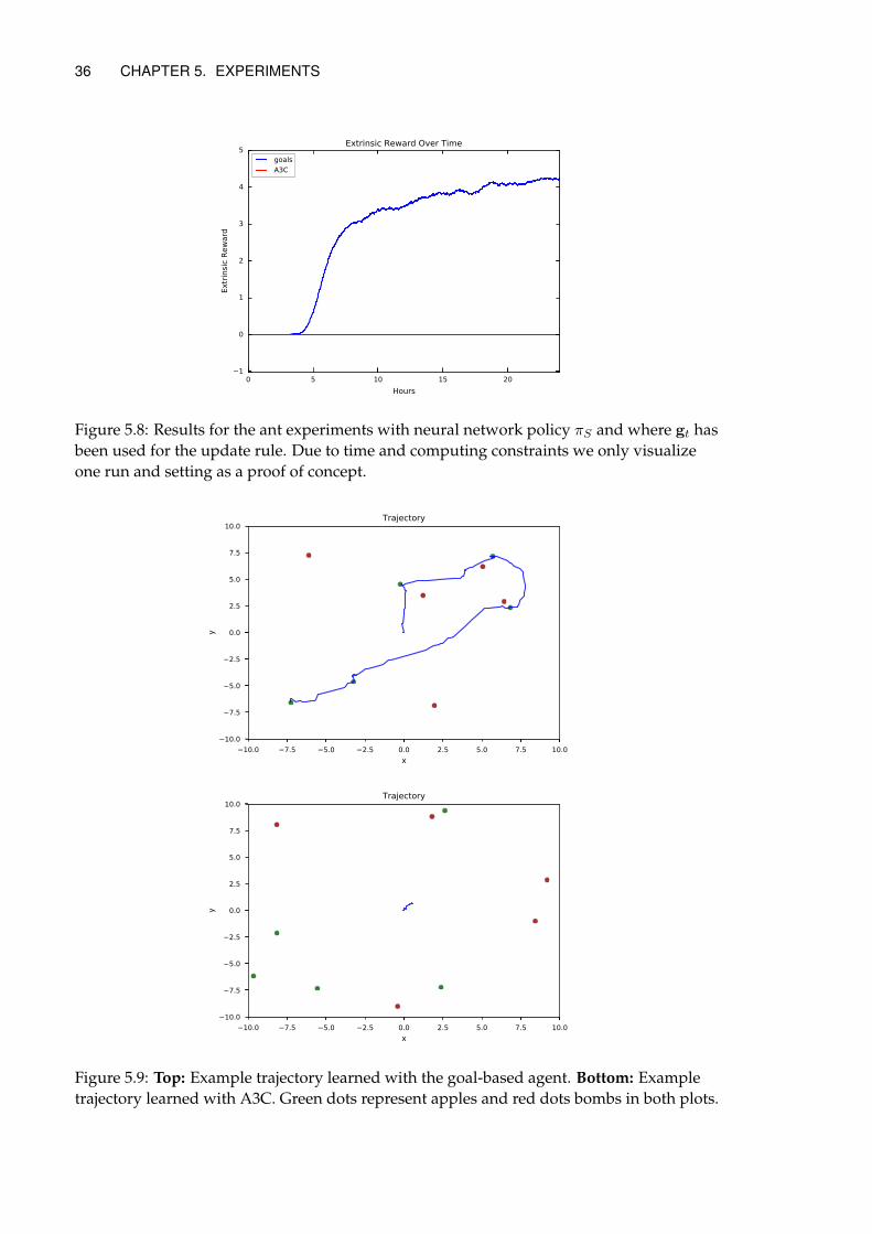
36 CHAPTER 5. EXPERIMENTS
0 5 10 15 20
Hours
1
0
1
2
3
4
5
Extr
insi
c R
ew
ard
Extrinsic Reward Over Time
goals
A3C
Figure 5.8: Results for the ant experiments with neural network policy πS and where gt has
been used for the update rule. Due to time and computing constraints we only visualize
one run and setting as a proof of concept.
10.0 7.5 5.0 2.5 0.0 2.5 5.0 7.5 10.0x
10.0
7.5
5.0
2.5
0.0
2.5
5.0
7.5
10.0
y
Trajectory
10.0 7.5 5.0 2.5 0.0 2.5 5.0 7.5 10.0x
10.0
7.5
5.0
2.5
0.0
2.5
5.0
7.5
10.0
y
Trajectory
Figure 5.9: Top: Example trajectory learned with the goal-based agent. Bottom: Example
trajectory learned with A3C. Green dots represent apples and red dots bombs in both plots.

CHAPTER 5. EXPERIMENTS 37
more able to set reachable goals more reliably. We expected, that using the reached state,
instead of the goal, in the update rule (refer Equation 4.2) would further improve the
ability to set reachable goals. However, as Figures 5.6 and 5.7 show, this was only ob-
served to a small extend. As seen in Figure 5.8 the approach scales readily from the point-
mass model to complex agents, as the ant of the MuJoCo benchmark.
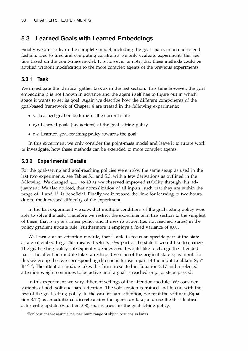
38 CHAPTER 5. EXPERIMENTS
5.3 Learned Goals with Learned Embeddings
Finally we aim to learn the complete model, including the goal space, in an end-to-end
fashion. Due to time and computing constraints we only evaluate experiments this sec-
tion based on the point-mass model. It is however to note, that these methods could be
applied without modification to the more complex agents of the previous experiments
5.3.1 Task
We investigate the identical gather task as in the last section. This time however, the goal
embedding φ is not known in advance and the agent itself has to figure out in which
space it wants to set its goal. Again we describe how the different components of the
goal-based framework of Chapter 4 are treated in the following experiments:
• φ: Learned goal embedding of the current state
• πS : Learned goals (i.e. actions) of the goal-setting policy
• πR: Learned goal-reaching policy towards the goal
In this experiment we only consider the point-mass model and leave it to future work
to investigate, how these methods can be extended to more complex agents.
5.3.2 Experimental Details
For the goal-setting and goal-reaching policies we employ the same setup as used in the
last two experiments, see Tables 5.1 and 5.3, with a few derivations as outlined in the
following. We changed gmax to 40 as we observed improved stability through this ad-
justment. We also noticed, that normalization of all inputs, such that they are within the
range of -1 and 11, is beneficial. Finally we increased the time for learning to two hours
due to the increased difficulty of the experiment.
In the last experiment we saw, that multiple conditions of the goal-setting policy were
able to solve the task. Therefore we restrict the experiments in this section to the simplest
of these, that is πS is a linear policy and it uses its action (i.e. not reached states) in the
policy gradient update rule. Furthermore it employs a fixed variance of 0.01.
We learn φ as an attention module, that is able to focus on specific part of the state
as a goal embedding. This means it selects what part of the state it would like to change.
The goal-setting policy subsequently decides how it would like to change the attended
part. The attention module takes a reshaped version of the original state st as input. For
this we group the two corresponding directions for each part of the input to obtain St ∈
R2×12. The attention module takes the form presented in Equation 3.17 and a selected
attention weight continues to be active until a goal is reached or gmax steps passed.
In this experiment we vary different settings of the attention module. We consider
variants of both soft and hard attention. The soft version is trained end-to-end with the
rest of the goal-setting policy. In the case of hard attention, we treat the softmax (Equa-
tion 3.17) as an additional discrete action the agent can take, and use the the identical
actor-critic update (Equation 3.8), that is used for the goal-setting policy.
1For locations we assume the maximum range of object locations as limits
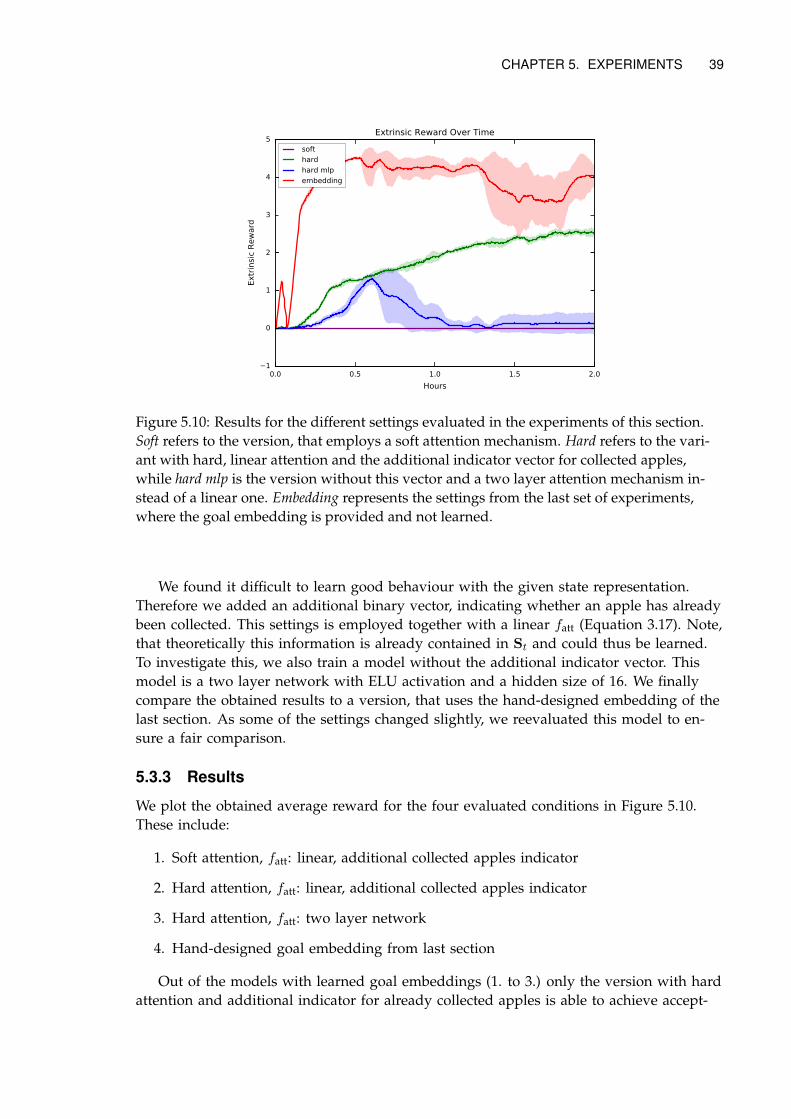
CHAPTER 5. EXPERIMENTS 39
0.0 0.5 1.0 1.5 2.0
Hours
1
0
1
2
3
4
5
Extr
insi
c R
ew
ard
Extrinsic Reward Over Time
soft
hard
hard mlp
embedding
Figure 5.10: Results for the different settings evaluated in the experiments of this section.
Soft refers to the version, that employs a soft attention mechanism. Hard refers to the vari-
ant with hard, linear attention and the additional indicator vector for collected apples,
while hard mlp is the version without this vector and a two layer attention mechanism in-
stead of a linear one. Embedding represents the settings from the last set of experiments,
where the goal embedding is provided and not learned.
We found it difficult to learn good behaviour with the given state representation.
Therefore we added an additional binary vector, indicating whether an apple has already
been collected. This settings is employed together with a linear fatt (Equation 3.17). Note,
that theoretically this information is already contained in St and could thus be learned.
To investigate this, we also train a model without the additional indicator vector. This
model is a two layer network with ELU activation and a hidden size of 16. We finally
compare the obtained results to a version, that uses the hand-designed embedding of the
last section. As some of the settings changed slightly, we reevaluated this model to en-
sure a fair comparison.
5.3.3 Results
We plot the obtained average reward for the four evaluated conditions in Figure 5.10.
These include:
1. Soft attention, fatt: linear, additional collected apples indicator
2. Hard attention, fatt: linear, additional collected apples indicator
3. Hard attention, fatt: two layer network
4. Hand-designed goal embedding from last section
Out of the models with learned goal embeddings (1. to 3.) only the version with hard
attention and additional indicator for already collected apples is able to achieve accept-
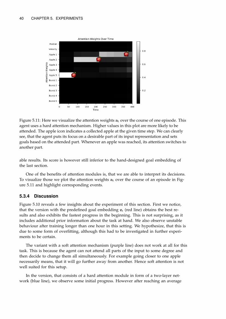
40 CHAPTER 5. EXPERIMENTS
Figure 5.11: Here we visualize the attention weights at over the course of one episode. This
agent uses a hard attention mechanism. Higher values in this plot are more likely to be
attended. The apple icon indicates a collected apple at the given time step. We can clearly
see, that the agent puts its focus on a desirable part of its input representation and sets
goals based on the attended part. Whenever an apple was reached, its attention switches to
another part.
able results. Its score is however still inferior to the hand-designed goal embedding of
the last section.
One of the benefits of attention modules is, that we are able to interpret its decisions.
To visualize those we plot the attention weights at over the course of an episode in Fig-
ure 5.11 and highlight corresponding events.
5.3.4 Discussion
Figure 5.10 reveals a few insights about the experiment of this section. First we notice,
that the version with the predefined goal embedding zt (red line) obtains the best re-
sults and also exhibits the fastest progress in the beginning. This is not surprising, as it
includes additional prior information about the task at hand. We also observe unstable
behaviour after training longer than one hour in this setting. We hypothesize, that this is
due to some form of overfitting, although this had to be investigated in further experi-
ments to be certain.
The variant with a soft attention mechanism (purple line) does not work at all for this
task. This is because the agent can not attend all parts of the input to some degree and
then decide to change them all simultaneously. For example going closer to one apple
necessarily means, that it will go further away from another. Hence soft attention is not
well suited for this setup.
In the version, that consists of a hard attention module in form of a two-layer net-
work (blue line), we observe some initial progress. However after reaching an average
CHAPTER 5. EXPERIMENTS 41
reward of one, the learned policy starts to diverge again. We try to explain this behaviour
with the following reasoning. A good agent is likely to put its attention on closeby ap-
ples. It then learns to get closer to one of these and eventually collects it. After this the
values of the corresponding entry will consist of zeros, indicating that the collected apple
is now carried. Attending already collected apples is something, that the agent should
avoid, if it wants to obtain further rewards. Now the agent is in a misery, it wants to at-
tend apples, with low absolute entries (meaning they are close to its position), but it also
wants to avoid entries, that are exactly zero (meaning it already collected the item). We
believe, that this sharp decision boundary is the reason for observed instabilities.
In order to evaluate this claim, we added an additional binary vector, indicating whether
an apple has already been collected or not, to the input (green line). In this setting we
observe, that the agent is able to learn a representation of its goal space through the hard
attention module. After two hours of training even the linear module achieves an aver-
age reward of around 2.5. It is to note, that this is still slightly less than the setting with
predefined goal representations obtains. While we have known such a representation for
the task at hand, there are many other cases where this form of prior knowledge is not
available. Using attention modules additionally adds potential to interpret the agents ac-
tions as we have illustrated in Figure 5.11.
Chapter 6
Conclusion and Future Work
In thesis we investigated whether Reinforcement Learning agents can be improved through
the addition of an explicit form of goal-directed behaviour. It was hypothesized, that
such a mechanism facilitates long-term credit assignment and provides improved explo-
ration capabilities. Because of that goal-directed behaviour might be especially useful in
environments with sparse reward signals.
We provided an introduction to the areas of Reinforcement Learning and Deep Learn-
ing, which are the core components of this work. Furthermore we summarized existing
literature on hierarchical Reinforcement Learning. We proposed a framework, based on
multiple deep networks, which learns to set goals on spaces, that are either specified by
the user or learned in an end-to-end manner. We have furthermore related the proposed
approach to existing literature through a connection with the options framework.
We evaluated the presented approach on a set of experiments of increasing difficulty.
This allowed to investigate all components of goal-directed learning in isolation, leading
to an incremental solution. While we focused on agents with continuous action spaces
and a gather scenario, the framework itself is not restricted to these settings and can be
applied in a wide range of other tasks.
Experimental analysis highlights, that all components of goal-based reasoning, includ-
ing identifying a suitable goal space, setting goals and finally reaching them, can be ob-
tained through a combination of RL with deep neural networks. Furthermore we show,
that the framework is able to solve challenging tasks, on which state-of-the-art RL algo-
rithms struggle to find good solutions.
Developing methods, that are able to act autonomously in complex tasks, is likely
to become of commercial importance in the upcoming years. It does not only enable to
solve problems more efficiently [86], but might also be the safer option in some scenarios
[87]. It is possible to view many use cases in industrial applications as sequential deci-
sion making problems. In this context it is often convenient to express success in a given
task through sparse reward functions. It is therefore crucial, that employed algorithms
are able to work well in this setting. The model proposed here directly relates to this, as
it has the potential to handle very sparse reward signals.
The lack of interpretability is often a concern when using neural networks. However,
due to the modularity of the approach proposed here, we can always replace indepen-
42
CHAPTER 6. CONCLUSION AND FUTURE WORK 43
dent components of the model, if we require additional safety guarantees. Additionally
we have shown, that it is possible to use an attention mechanism for learning the goal
representation, which allows us to inspect some of the decisions within the model.
There are many possible ways to improve the approach presented here. Some of the
challenges are related to the goal-setting policy. This includes for example the update
rule when learning with a policy gradient-based algorithm. Additionally it is an open
question if random Gaussian exploration is a suitable choice when dealing with high-
level goals or if alternatives should be considered. It would be also desirable to have an
adaptive step-size gmax for different goals.
Ideally we would like to have more data-efficient algorithms, especially when apply-
ing these methods on real robots. This might turn out to be crucial for the goal-setting
policy, as it is, by design, exposed to less data. Model-based approaches are inherently
data-efficient [88] and thus might provide one solution to overcome this issue. Note, that
it very natural to learn a model for the goal-setting agent based on transitions in goal
space. This is because we are likely to know, where will end up after setting a goal (un-
der the assumption, that the goal-reaching policy actually implements behaviour that
leads to the chosen goal).
It will also be interesting to see how the results of the end-to-end trainable models
from Section 5.3 transfer to more challenging agents. Furthermore it is desirable to ap-
ply these methods to a set of different tasks, such as maze navigation or game playing,
including cases where only raw visual observations are provided. It remains to be seen,
whether we should strive to design such a system by hand or if we can discover meth-
ods, that are able to automate this process.
Bibliography
[1] Volodymyr Mnih, Koray Kavukcuoglu, David Silver, Andrei A Rusu, Joel Veness,
Marc G Bellemare, Alex Graves, Martin Riedmiller, Andreas K Fidjeland, Georg Os-
trovski, et al. Human-level control through deep reinforcement learning. Nature, 518
(7540):529–533, 2015.
[2] Shixiang Gu, Ethan Holly, Timothy P. Lillicrap, and Sergey Levine. Deep rein-
forcement learning for robotic manipulation. CoRR, abs/1610.00633, 2016. URL
http://arxiv.org/abs/1610.00633.
[3] David Silver, Aja Huang, Chris J Maddison, Arthur Guez, Laurent Sifre, George
Van Den Driessche, Julian Schrittwieser, Ioannis Antonoglou, Veda Panneershelvam,
Marc Lanctot, et al. Mastering the game of go with deep neural networks and tree
search. Nature, 529(7587):484–489, 2016.
[4] Marc Bellemare, Yavar Naddaf, Joel Veness, and Michael Bowling. The arcade learn-
ing environment: An evaluation platform for general agents. In Twenty-Fourth Inter-
national Joint Conference on Artificial Intelligence, 2015.
[5] Volodymyr Mnih, Adria Puigdomenech Badia, Mehdi Mirza, Alex Graves, Timo-
thy P Lillicrap, Tim Harley, David Silver, and Koray Kavukcuoglu. Asynchronous
methods for deep reinforcement learning. arXiv preprint arXiv:1602.01783, 2016.
[6] Paul FMJ Verschure, Cyriel MA Pennartz, and Giovanni Pezzulo. The why, what,
where, when and how of goal-directed choice: neuronal and computational princi-
ples. Phil. Trans. R. Soc. B, 369(1655):20130483, 2014.
[7] Henk Aarts and Andrew Elliot. Goal-directed behavior. Taylor & Francis, 2012.
[8] Yukiori Goto and Anthony A Grace. Dopaminergic modulation of limbic and corti-
cal drive of nucleus accumbens in goal-directed behavior. Nature neuroscience, 8(6):
805–812, 2005.
[9] Matthew M Botvinick, Yael Niv, and Andrew C Barto. Hierarchically organized be-
havior and its neural foundations: A reinforcement learning perspective. Cognition,
113(3):262–280, 2009.
[10] Shixiang Gu, Timothy P. Lillicrap, Ilya Sutskever, and Sergey Levine. Continuous
deep q-learning with model-based acceleration. CoRR, abs/1603.00748, 2016. URL
http://arxiv.org/abs/1603.00748.
44
BIBLIOGRAPHY 45
[11] John Schulman, Sergey Levine, Philipp Moritz, Michael I. Jordan, and Pieter
Abbeel. Trust region policy optimization. CoRR, abs/1502.05477, 2015. URL
http://arxiv.org/abs/1502.05477.
[12] Ziyu Wang, Victor Bapst, Nicolas Heess, Volodymyr Mnih, Remi Munos, Koray
Kavukcuoglu, and Nando de Freitas. Sample efficient actor-critic with experience
replay. arXiv preprint arXiv:1611.01224, 2016.
[13] Shixiang Gu, Timothy P. Lillicrap, Zoubin Ghahramani, Richard E. Turner, and
Sergey Levine. Q-prop: Sample-efficient policy gradient with an off-policy critic.
CoRR, abs/1611.02247, 2016. URL http://arxiv.org/abs/1611.02247.
[14] Guy Lever. Deterministic policy gradient algorithms. 2014.
[15] Timothy P Lillicrap, Jonathan J Hunt, Alexander Pritzel, Nicolas Heess, Tom Erez,
Yuval Tassa, David Silver, and Daan Wierstra. Continuous control with deep rein-
forcement learning. arXiv preprint arXiv:1509.02971, 2015.
[16] John Schulman, Philipp Moritz, Sergey Levine, Michael Jordan, and Pieter Abbeel.
High-dimensional continuous control using generalized advantage estimation. arXiv
preprint arXiv:1506.02438, 2015.
[17] Max Jaderberg, Volodymyr Mnih, Wojciech Marian Czarnecki, Tom Schaul, Joel Z
Leibo, David Silver, and Koray Kavukcuoglu. Reinforcement learning with unsuper-
vised auxiliary tasks. arXiv preprint arXiv:1611.05397, 2016.
[18] Emanuel Todorov, Tom Erez, and Yuval Tassa. Mujoco: A physics engine for model-
based control. In Intelligent Robots and Systems (IROS), 2012 IEEE/RSJ International
Conference on, pages 5026–5033. IEEE, 2012.
[19] Yan Duan, Xi Chen, Rein Houthooft, John Schulman, and Pieter Abbeel. Benchmark-
ing deep reinforcement learning for continuous control. CoRR, abs/1604.06778, 2016.
URL http://arxiv.org/abs/1604.06778.
[20] Peter Dayan and Geoffrey E Hinton. Feudal reinforcement learning. In Advances in
neural information processing systems, pages 271–271. Morgan Kaufmann Publishers,
1993.
[21] Tejas D. Kulkarni, Karthik Narasimhan, Ardavan Saeedi, and Joshua B. Tenen-
baum. Hierarchical deep reinforcement learning: Integrating temporal ab-
straction and intrinsic motivation. CoRR, abs/1604.06057, 2016. URL
http://arxiv.org/abs/1604.06057.
[22] A. Sasha Vezhnevets, S. Osindero, T. Schaul, N. Heess, M. Jaderberg, D. Silver, and
K. Kavukcuoglu. FeUdal Networks for Hierarchical Reinforcement Learning. ArXiv
e-prints, March 2017.
[23] Bram Bakker and Jürgen Schmidhuber. Hierarchical reinforcement learning based on
subgoal discovery and subpolicy specialization. In Proc. of the 8-th Conf. on Intelligent
Autonomous Systems, pages 438–445, 2004.
46 BIBLIOGRAPHY
[24] Xue Bin Peng, Glen Berseth, KangKang Yin, and Michiel van de Panne. Deeploco:
Dynamic locomotion skills using hierarchical deep reinforcement learning. ACM
Transactions on Graphics (Proc. SIGGRAPH 2017), 36(4), 2017.
[25] Richard S Sutton, Doina Precup, and Satinder Singh. Between mdps and semi-mdps:
A framework for temporal abstraction in reinforcement learning. Artificial intelligence,
112(1):181–211, 1999.
[26] Marlos C. Machado and Michael H. Bowling. Learning purposeful be-
haviour in the absence of rewards. CoRR, abs/1605.07700, 2016. URL
http://arxiv.org/abs/1605.07700.
[27] Aravind S Lakshminarayanan, Ramnandan Krishnamurthy, Peeyush Kumar, and
Balaraman Ravindran. Option discovery in hierarchical reinforcement learning using
spatio-temporal clustering. arXiv preprint arXiv:1605.05359, 2016.
[28] Amy McGovern and Andrew G Barto. Automatic discovery of subgoals in reinforce-
ment learning using diverse density. 2001.
[29] Pierre-Luc Bacon, Jean Harb, and Doina Precup. The option-critic architecture. arXiv
preprint arXiv:1609.05140, 2016.
[30] Tom Schaul, Daniel Horgan, Karol Gregor, and David Silver. Universal value func-
tion approximators. In Proceedings of the 32nd International Conference on Machine Learn-
ing (ICML-15), pages 1312–1320, 2015.
[31] Yuke Zhu, Roozbeh Mottaghi, Eric Kolve, Joseph J Lim, Abhinav Gupta, Li Fei-Fei,
and Ali Farhadi. Target-driven visual navigation in indoor scenes using deep rein-
forcement learning. arXiv preprint arXiv:1609.05143, 2016.
[32] Jingwei Zhang, Jost Tobias Springenberg, Joschka Boedecker, and Wolfram Burgard.
Deep reinforcement learning with successor features for navigation across similar
environments. arXiv preprint arXiv:1612.05533, 2016.
[33] Alexey Dosovitskiy and Vladlen Koltun. Learning to act by predicting the future.
arXiv preprint arXiv:1611.01779, 2016.
[34] Thomas G Dietterich. Hierarchical reinforcement learning with the maxq value func-
tion decomposition. J. Artif. Intell. Res.(JAIR), 13:227–303, 2000.
[35] Ronald Parr and Stuart Russell. Reinforcement learning with hierarchies of ma-
chines.
[36] Doina Precup, Richard S Sutton, and Satinder P Singh. Planning with closed-loop
macro actions. In Working notes of the 1997 AAAI Fall Symposium on Model-directed Au-
tonomous Systems, pages 70–76, 1997.
[37] Amy McGovern, Richard S Sutton, and Andrew H Fagg. Roles of macro-actions in
accelerating reinforcement learning. In Grace Hopper celebration of women in computing,
volume 1317, 1997.
BIBLIOGRAPHY 47
[38] Alexander Vezhnevets, Volodymyr Mnih, Simon Osindero, Alex Graves, Oriol
Vinyals, John Agapiou, et al. Strategic attentive writer for learning macro-actions.
In Advances in Neural Information Processing Systems, pages 3486–3494, 2016.
[39] Richard S Sutton, Joseph Modayil, Michael Delp, Thomas Degris, Patrick M Pilarski,
Adam White, and Doina Precup. Horde: A scalable real-time architecture for learn-
ing knowledge from unsupervised sensorimotor interaction. In The 10th International
Conference on Autonomous Agents and Multiagent Systems-Volume 2, pages 761–768. In-
ternational Foundation for Autonomous Agents and Multiagent Systems, 2011.
[40] Alexander L Strehl and Michael L Littman. An analysis of model-based interval
estimation for markov decision processes. Journal of Computer and System Sciences, 74
(8):1309–1331, 2008.
[41] Haoran Tang, Rein Houthooft, Davis Foote, Adam Stooke, Xi Chen, Yan Duan, John
Schulman, Filip De Turck, and Pieter Abbeel. #exploration: A study of count-based
exploration for deep reinforcement learning. CoRR, abs/1611.04717, 2016. URL
http://arxiv.org/abs/1611.04717.
[42] Marc Bellemare, Sriram Srinivasan, Georg Ostrovski, Tom Schaul, David Saxton, and
Remi Munos. Unifying count-based exploration and intrinsic motivation. In Ad-
vances in Neural Information Processing Systems, pages 1471–1479, 2016.
[43] Georg Ostrovski, Marc G Bellemare, Aaron van den Oord, and Remi Munos. Count-
based exploration with neural density models. arXiv preprint arXiv:1703.01310, 2017.
[44] Yarin Gal. Uncertainty in Deep Learning. PhD thesis, University of Cambridge, 2016.
[45] William R Thompson. On the likelihood that one unknown probability exceeds an-
other in view of the evidence of two samples. Biometrika, 25(3/4):285–294, 1933.
[46] Rein Houthooft, Xi Chen, Yan Duan, John Schulman, Filip De Turck, and
Pieter Abbeel. Curiosity-driven exploration in deep reinforcement learn-
ing via bayesian neural networks. CoRR, abs/1605.09674, 2016. URL
http://arxiv.org/abs/1605.09674.
[47] Yi Sun, Faustino Gomez, and Jürgen Schmidhuber. Planning to be surprised: Op-
timal bayesian exploration in dynamic environments. In International Conference on
Artificial General Intelligence, pages 41–51. Springer, 2011.
[48] J. Achiam and S. Sastry. Surprise-Based Intrinsic Motivation for Deep Reinforcement
Learning. ArXiv e-prints, March 2017.
[49] George Cybenko. Approximation by superpositions of a sigmoidal function. Mathe-
matics of Control, Signals, and Systems (MCSS), 2(4):303–314, 1989.
[50] Kurt Hornik. Approximation capabilities of multilayer feedforward networks. Neural
networks, 4(2):251–257, 1991.
[51] Richard S Sutton and Andrew G Barto. Reinforcement learning: An introduction, vol-
ume 1. MIT press Cambridge, 1998.
48 BIBLIOGRAPHY
[52] John P O’Doherty, Peter Dayan, Karl Friston, Hugo Critchley, and Raymond J Dolan.
Temporal difference models and reward-related learning in the human brain. Neu-
ron, 38(2):329–337, 2003.
[53] Richard S Sutton, David A McAllester, Satinder P Singh, Yishay Mansour, et al. Pol-
icy gradient methods for reinforcement learning with function approximation. In
NIPS, volume 99, pages 1057–1063, 1999.
[54] Jack PC Kleijnen and Reuven Y Rubinstein. Optimization and sensitivity analysis
of computer simulation models by the score function method. European Journal of
Operational Research, 88(3):413–427, 1996.
[55] Ronald J Williams. Simple statistical gradient-following algorithms for connectionist
reinforcement learning. Machine learning, 8(3-4):229–256, 1992.
[56] Long-Ji Lin. Reinforcement learning for robots using neural networks. Technical
report, DTIC Document, 1993.
[57] F. Niu, B. Recht, C. Re, and S. J. Wright. HOGWILD!: A Lock-Free Approach to Par-
allelizing Stochastic Gradient Descent. ArXiv e-prints, June 2011.
[58] Ronald J Williams and Jing Peng. Function optimization using connectionist rein-
forcement learning algorithms. Connection Science, 3(3):241–268, 1991.
[59] John N Tsitsiklis, Benjamin Van Roy, et al. An analysis of temporal-difference learn-
ing with function approximation. IEEE transactions on automatic control, 42(5):674–690,
1997.
[60] Yaakov Engel, Shie Mannor, and Ron Meir. Reinforcement learning with gaussian
processes. In Proceedings of the 22nd international conference on Machine learning, pages
201–208. ACM, 2005.
[61] Carl Edward Rasmussen, Malte Kuss, et al. Gaussian processes in reinforcement
learning. In NIPS, volume 4, page 1, 2003.
[62] Ian Goodfellow, Yoshua Bengio, and Aaron Courville. Deep Learning. MIT Press,
2016. http://www.deeplearningbook.org.
[63] Richard HR Hahnloser, Rahul Sarpeshkar, Misha A Mahowald, Rodney J Douglas,
and H Sebastian Seung. Digital selection and analogue amplification coexist in a
cortex-inspired silicon circuit. Nature, 405(6789):947–951, 2000.
[64] Djork-Arné Clevert, Thomas Unterthiner, and Sepp Hochreiter. Fast and ac-
curate deep network learning by exponential linear units (elus). arXiv preprint
arXiv:1511.07289, 2015.
[65] Kaiming He, Xiangyu Zhang, Shaoqing Ren, and Jian Sun. Deep resid-
ual learning for image recognition. CoRR, abs/1512.03385, 2015. URL
http://arxiv.org/abs/1512.03385.
[66] Rupesh Kumar Srivastava, Klaus Greff, and Jürgen Schmidhuber. Highway net-
works. arXiv preprint arXiv:1505.00387, 2015.
BIBLIOGRAPHY 49
[67] Yoshua Bengio et al. Learning deep architectures for ai. Foundations and trends R© in
Machine Learning, 2(1):1–127, 2009.
[68] Alex Graves. Supervised sequence labelling. In Supervised Sequence Labelling with
Recurrent Neural Networks, pages 5–13. Springer, 2012.
[69] Jeffrey L Elman. Finding structure in time. Cognitive science, 14(2):179–211, 1990.
[70] Yonghui Wu, Mike Schuster, Zhifeng Chen, Quoc V. Le, Mohammad Norouzi, Wolf-
gang Macherey, Maxim Krikun, Yuan Cao, Qin Gao, Klaus Macherey, Jeff Klingner,
Apurva Shah, Melvin Johnson, Xiaobing Liu, Lukasz Kaiser, Stephan Gouws,
Yoshikiyo Kato, Taku Kudo, Hideto Kazawa, Keith Stevens, George Kurian, Nishant
Patil, Wei Wang, Cliff Young, Jason Smith, Jason Riesa, Alex Rudnick, Oriol Vinyals,
Greg Corrado, Macduff Hughes, and Jeffrey Dean. Google’s neural machine trans-
lation system: Bridging the gap between human and machine translation. CoRR,
abs/1609.08144, 2016. URL http://arxiv.org/abs/1609.08144.
[71] Dario Amodei, Rishita Anubhai, Eric Battenberg, Carl Case, Jared Casper, Bryan
Catanzaro, Jingdong Chen, Mike Chrzanowski, Adam Coates, Greg Diamos,
Erich Elsen, Jesse Engel, Linxi Fan, Christopher Fougner, Tony Han, Awni Y.
Hannun, Billy Jun, Patrick LeGresley, Libby Lin, Sharan Narang, Andrew Y. Ng,
Sherjil Ozair, Ryan Prenger, Jonathan Raiman, Sanjeev Satheesh, David Seeta-
pun, Shubho Sengupta, Yi Wang, Zhiqian Wang, Chong Wang, Bo Xiao, Dani
Yogatama, Jun Zhan, and Zhenyao Zhu. Deep speech 2: End-to-end speech
recognition in english and mandarin. CoRR, abs/1512.02595, 2015. URL
http://arxiv.org/abs/1512.02595.
[72] Sepp Hochreiter, Yoshua Bengio, Paolo Frasconi, and Jürgen Schmidhuber. Gradient
flow in recurrent nets: the difficulty of learning long-term dependencies, 2001.
[73] Sepp Hochreiter and Jürgen Schmidhuber. Long short-term memory. Neural computa-
tion, 9(8):1735–1780, 1997.
[74] David E Rumelhart, Geoffrey E Hinton, and Ronald J Williams. Learning representa-
tions by back-propagating errors. Cognitive modeling, 5(3):1, 1988.
[75] T. Tieleman and G. Hinton. RMSprop Gradient Optimization. URL
http://www.cs.toronto.edu/˜tijmen/csc321/slides/lecture_slides_lec6.pdf.
[76] Diederik P. Kingma and Jimmy Ba. Adam: A method for stochastic optimization.
CoRR, abs/1412.6980, 2014. URL http://arxiv.org/abs/1412.6980.
[77] Paul J Werbos. Generalization of backpropagation with application to a recurrent
gas market model. Neural networks, 1(4):339–356, 1988.
[78] Dzmitry Bahdanau, Kyunghyun Cho, and Yoshua Bengio. Neural machine transla-
tion by jointly learning to align and translate. arXiv preprint arXiv:1409.0473, 2014.
[79] Kyunghyun Cho, Aaron Courville, and Yoshua Bengio. Describing multimedia con-
tent using attention-based encoder-decoder networks. IEEE Transactions on Multime-
dia, 17(11):1875–1886, 2015.
50 BIBLIOGRAPHY
[80] Kelvin Xu, Jimmy Ba, Ryan Kiros, Kyunghyun Cho, Aaron Courville, Ruslan
Salakhudinov, Rich Zemel, and Yoshua Bengio. Show, attend and tell: Neural im-
age caption generation with visual attention. In International Conference on Machine
Learning, pages 2048–2057, 2015.
[81] Bram Bakker and Jürgen Schmidhuber. Hierarchical reinforcement learning based on
subgoal discovery and subpolicy specialization. In Proceedings of the 8-th Conference on
Intelligent Autonomous Systems, IAS-8, pages 438–445, 2004.
[82] E. Jang, S. Gu, and B. Poole. Categorical Reparameterization with Gumbel-Softmax.
ArXiv e-prints, November 2016.
[83] Pawel Wawrzynski. Learning to control a 6-degree-of-freedom walking robot. In
EUROCON, 2007. The International Conference on" Computer as a Tool", pages 698–705.
IEEE, 2007.
[84] Greg Brockman, Vicki Cheung, Ludwig Pettersson, Jonas Schneider, John Schulman,
Jie Tang, and Wojciech Zaremba. Openai gym, 2016.
[85] PyTorch. http://pytorch.org/. Accessed: 2017-04-16.
[86] Jim Gao and Ratnesh Jamidar. Machine learning applications for data center opti-
mization. Google White Paper, 2014.
[87] A Hussain, A Malik, MU Halim, and AM Ali. The use of robotics in surgery: a re-
view. International journal of clinical practice, 68(11):1376–1382, 2014.
[88] Marc Deisenroth and Carl E Rasmussen. Pilco: A model-based and data-efficient
approach to policy search. In Proceedings of the 28th International Conference on machine
learning (ICML-11), pages 465–472, 2011.

www.kth.se
Powered by TCPDF (www.tcpdf.org)Powered by TCPDF (www.tcpdf.org)Powered by TCPDF (www.tcpdf.org)Powered by TCPDF (www.tcpdf.org)Powered by TCPDF (www.tcpdf.org)Powered by TCPDF (www.tcpdf.org)Powered by TCPDF (www.tcpdf.org)Powered by TCPDF (www.tcpdf.org)Powered by TCPDF (www.tcpdf.org)Powered by TCPDF (www.tcpdf.org)Powered by TCPDF (www.tcpdf.org)