learning hierarchical sparse features for rgb-(d) object recognition

Article

Learning hierarchical sparse features forRGB-(D) object recognition

The International Journal ofRobotics Research2014, Vol. 33(4) 581–599© The Author(s) 2014Reprints and permissions:sagepub.co.uk/journalsPermissions.navDOI: 10.1177/0278364913514283ijr.sagepub.com

Liefeng Bo1,2, Xiaofeng Ren1 and Dieter Fox2

AbstractRecently introduced RGB-D cameras are capable of providing high quality synchronized videos of both color and depth.With its advanced sensing capabilities, this technology represents an opportunity to significantly increase the capabilitiesof object recognition. It also raises the problem of developing expressive features for the color and depth channels ofthese sensors. In this paper we introduce hierarchical matching pursuit (HMP) for RGB-D data. As a multi-layer sparsecoding network, HMP builds feature hierarchies layer by layer with an increasing receptive field size to capture abstractrepresentations from raw RGB-D data. HMP uses sparse coding to learn codebooks at each layer in an unsupervisedway and builds hierarchical feature representations from the learned codebooks in conjunction with orthogonal matchingpursuit, spatial pooling and contrast normalization. Extensive experiments on various datasets indicate that the featureslearned with our approach enable superior object recognition results using linear support vector machines.

KeywordsObject recognition, feature learning, sparse coding, hierarchical segmentation, RGB-D cameras

1. Introduction

Recognizing object instances and categories is a crucialcapability for an autonomous robot to understand and inter-act with the physical world. Only by recognizing objects cana robot reason about their affordances, manipulate them ina purposeful way, and understand commands given in nat-ural language, such as “Put the dirty cereal bowl into thedish washer”. Because of its importance, object recognitionhas recently received substantial attention in the roboticscommunity. Humans are able to recognize objects despitelarge variation in their appearance due to changing view-points, scales, lighting conditions and deformations. Thisability fundamentally relies on robust visual representationsof the physical world. However, most state-of-the-art objectrecognition systems are still based on manually designedrepresentations (features), such as SIFT (Lowe, 2004),HOG (Dalal and Triggs, 2005), Spin Images (Johnson andHebert, 1999), SURF (Bay et al., 2008), Fast Point Fea-ture Histogram (Morisset et al., 2009), LINE-MOD (Hin-terstoisser et al., 2011), or feature combinations (Lai et al.,2011a). Such approaches suffer from at least two key lim-itations. Firstly, these features usually only capture a smallset of recognition cues from raw data; other useful cues areignored during feature design. For instance, the well-knownSIFT features capture edge information from RGB imagesusing a pair of horizontal and vertical gradient filters while

completely ignoring color information. Secondly, the fea-tures have to be re-designed for new data types, or even newtasks, making object recognition systems heavily dependenton expert experience. It is desirable to develop efficientand effective machine learning algorithms to automaticallyextract robust representations from raw sensor data.

Instead of manually designing features, feature learn-ing aims to transform raw data to expressive features withwhich tasks such as classification can be solved more accu-rately. This approach is attractive as it exploits the availabil-ity of a large amount of unlabeled data and avoids the needof feature engineering, and recently it has become increas-ingly popular and effective for object recognition. In thelast few years, a variety of feature learning techniques havebeen developed (Hinton et al., 2006; Lee et al., 2009; Wanget al., 2010; Bo et al., 2011c). Algorithms such as deepbelief nets, convolutional deep belief networks, convolu-tional neural networks, deep autoencoders, recursive neuralnetworks, k-means based feature learning, and sparse cod-ing have been proposed to this end. Such approaches build

1ISTC-Pervasive Computing Intel Labs, Seattle, USA2University of Washington, Seattle, USA

Corresponding author:Liefeng Bo, Box 352350, 101 Paul G. Allen Center for CSE446 Seattle,Washington 98105, USA.Email: [email protected]

at TEXAS SOUTHERN UNIVERSITY on December 16, 2014ijr.sagepub.comDownloaded from

http://ijr.sagepub.com/

582 The International Journal of Robotics Research 33(4)

feature hierarchies from scratch, and have exhibited veryimpressive performance on many types of recognition tasksincluding handwritten digit recognition, face recognition,tiny image recognition, object recognition, and scene recog-nition. Though very successful, the current vision appli-cations are somewhat limited to 2D images, typically ingrayscale.

Recently introduced low-cost RGB-D cameras are capa-ble of providing high quality synchronized videos of bothcolor and depth. The registered color and depth have poten-tial to boost a wide range of robotics applications. Forinstance, the Microsoft Kinect sensor, developed by Prime-Sense, provides 640 × 480 color and depth images at 30frames per second and has been successfully used for com-puter gaming (Shotton et al., 2011) and 3D reconstruc-tion (Henry et al., 2010; Newcombe et al., 2011). Withits advanced sensing capabilities, this technology repre-sents an opportunity to dramatically increase the capabil-ities of object recognition and manipulation as well. Overthe past few years, the robotics community has made sub-stantial progress in recognizing pre-segmented objects (Boet al., 2011b; Lai et al., 2011a; Tang et al., 2012), detectingobjects from cluttered scenes (Hinterstoisser et al., 2011;Lai et al., 2011a), and labeling objects in 3D point-cloudsfrom RGB-D video sequences (Anand et al., 2012; Laiet al., 2012a; Jiang et al., 2012). Though very promising,these approaches are still built on designed feature sets thatcould bound the overall performance of the whole system.This raises the problem of developing expressive featuresfor the color and depth channels of RGB-D sensors.

In this paper, we propose hierarchical matching pursuit(HMP) to learn features from scratch for color and depthimages captured by RGB-D cameras. HMP is a multi-layersparse coding network that builds feature hierarchies fromraw RGB-D data layer by layer with an increasing recep-tive field size. In particular, HMP learns codebooks at eachlayer via K-SVD (Aharon et al., 2006) in order to rep-resent patches or pooled sparse codes as a sparse, linearcombination of codebook entries (codewords). With thelearned dictionary, feature hierarchies are built, layer bylayer, using three components: orthogonal matching pursuit,spatial pooling, and contrast normalization. We discuss thearchitecture of HMP, and show that all three componentsand hierarchical structure are critical for learning good fea-tures for object recognition. We further present batch treeorthogonal matching pursuit to speed up the computation ofsparse codes by pre-computing quantities shared by a largenumber of image patches.

Extensive evaluations on several publicly availablebenchmark datasets enable us to gain various experimentalinsights: features learned from raw data can yield recog-nition accuracy that is superior to state-of-the-art objectrecognition algorithms, even to ones specifically designedand tuned for textured objects (Tang et al., 2012); HMPcan take full advantage of the additional information con-tained in color and depth channels and significantly boosts

the performance of RGB-D based object recognition. Wealso present results showing that HMP can be combinedwith a state-of-the-art segmentation technique to achievevery good performance on object detection, which is closerto realistic robotics applications.

This paper is organized as follows. Section 2 reviewsrelated work. Our feature learning approach, HMP, is pre-sented in Section 3, followed by an extensive experimentalevaluation in Section 4. We conclude in Section 5.

2. Related work

This research focuses on hierarchical feature learning forRGB-D object recognition and detection. In the past fewyears, a growing amount of research on object recognitionhas focused on learning rich features using unsupervisedlearning, supervised learning, hierarchical architectures,and their combination.

2.1. RGB-D object recognition and detection

Low-cost RGB-D cameras have dramatically increased thecapabilities of object recognition and detection. Kinectmakes the human body a controller by enabling accuratereal-time human pose estimation (Shotton et al., 2011). Laiet al. (2011a) collected an RGB-D Object Dataset usinga Kinect style camera, and investigated classical bag-of-words based object recognition and sliding window basedobject detection using designed shape and color featuresextracted from a single RGB-D frame. Tang et al. (2012)combine SIFT feature matching and geometric verificationto recognize highly textured object instances, and won theICRA 2011 Solutions in Perception instance recognitionchallenge. Hinterstoisser et al. (2011) proposed a templatebased approach for real-time object detection by quantiz-ing gradient orientations computed on a grayscale imageand surface normals computed on a depth image into inte-ger values. Object recognition and detection can be fur-ther improved by leveraging the geometric information ofthe reconstructed 3D scene, i.e. 3D point clouds. Anandet al. (2012) detect commonly found objects in the 3Dpoint cloud of indoor scenes obtained from RGB-D cam-eras. The approach exploits a graphical model to capturevarious features and contextual relations, including localvisual appearance and shape cues, object co-occurence rela-tionships and geometric relationships, and achieves goodaccuracy in labeling office and home scenes. Lai et al.(2012a) utilize sliding window detectors trained from RGB-D frames to assign probabilities to voxels in a reconstructed3D scene. A Markov Random Field is then applied to labelvoxels by combining cues from view-based detection and3D shape. Jiang et al. (2012) proposed a supervised learn-ing approach for detecting good placements from the givenpoint clouds of an object and the placing area. The approachlearns to combine the features that capture support, stability,and preferred placements using a shared sparsity structure



Bo et al. 583

in the parameters, and enables a robot to stably place severalnew objects in several new placing areas.

2.2. Deep networks

Since a 2006 breakthrough by Hinton et al. (2006), deeplearning has evolved as a popular machine learning tool forimage recognition. Deep belief nets (Hinton et al., 2006)build a hierarchy of features layer by layer using the unsu-pervised restricted Boltzmann machine. The procedure iscalled pre-training and very helpful for avoiding shallowlocal minima. The found weights are then fed to multi-layerfeed-forward neural networks and further adjusted to thecurrent task using supervised information. To make deepbelief nets applicable to full-size images, Lee et al. (2009)proposed convolutional deep belief nets that use a smallreceptive field and share the weights between the hiddenand visible layers among all locations in an image by adapt-ing the idea of convolutional neural networks (LeCun andHaffner, 1998). Deconvolutional networks (Zeiler et al.,2011) convolutionally decompose images in an unsuper-vised way under a sparsity constraint. By building a hier-archy of such decompositions, robust representations canbe built from raw images for image recognition. Tiled con-volutional neural networks (Le et al., 2011) are a typeof sparse deep architecture with three important ingredi-ents: local receptive fields, pooling, and local contrast nor-malization that enjoy the benefit of significantly reducingthe number of learnable parameters while giving the algo-rithm flexibility to learn invariant features. Recent work (Leet al., 2012) has shown that such deep networks can buildhigh-level, class-specific feature detectors from a large col-lection of unlabeled images, for instance human and catface detectors. Very recently, deep convolutional neuralnetworks have achieved impressive results on the latestImageNet challenge and demonstrated its potential for rec-ognizing images (Krizhevsky et al., 2012). In addition toimage recognition, recursive neural networks (Socher et al.,2011) have shown promising results for semantical scenelabeling by leveraging recursive structure in natural sceneimages. The key idea is to compute a score for mergingneighboring regions into a larger region, a new semanticfeature representation for this larger region, and its classlabel.

2.3. Sparse coding

For many years, sparse coding (Olshausen and Field, 1996)has been a popular tool for modeling images. Sparse cod-ing on top of raw image patches has been applied not onlyfor image processing including image denoising (Elad andAharon, 2006a), image compression (Donoho, 2006), andsuper-resolution (Yang et al., 2008), but also for imagerecognition including face recognition (Wright et al., 2009),digit recognition (Mairal et al., 2008b), and texture seg-mentation (Mairal et al., 2008a). More recently, it has

been shown that combining sparse coding with successfulimage features dramatically boosts image recognition. Forinstance, sparse coding on top of SIFT features achievesstate-of-the-art performance on challenging object recogni-tion benchmarks (Yang et al., 2009). Yang et al. (2009) firstproposed sparse coding over SIFT features rather than rawimage patches for image recognition, and demonstrated thatit significantly outperforms popular bag-of-visual-wordsmodels. Wang et al. (2010) presented a fast local coordinatecoding scheme for recognizing images, and the approachcomputes sparse codes of SIFT features by performing locallinear embedding on several nearest codewords in a code-book learned by k-means. Boureau et al. (2010) comparedmany types of object recognition algorithms, and foundthat SIFT based sparse coding followed by spatial pyra-mid max pooling are the best-performing approaches, andmacrofeatures can increase recognition accuracy even fur-ther. Coates and Ng (2011b) evaluated many sparse codingapproaches by decomposing them into training and encod-ing phases, and suggested that the choice of architecture andencoder is the key to a feature learning system. Sparse cod-ing requires a computationally expensive optimization stagefor computing sparse codes, which makes it infeasible forreal-time applications. Invariant predictive sparse decom-position (Jarrett et al., 2009; Kavukcuoglu et al., 2010)approximates sparse codes using multi-layer feed-forwardneural networks and avoids solving expensive optimiza-tions at runtime. Bo et al. (2011c) proposed a batch treeorthogonal matching pursuit to speed up the computationof sparse codes. The approach can handle full-size imagesefficiently, and is particularly suitable for encoding a largenumber of observations that share the same large dictionary.Inspired by deep networks, multi-layer sparse coding net-works including hierarchical sparse coding (Yu et al., 2011)and HMP (Bo et al., 2011c, 2013) have been proposed forbuilding hierarchical features from raw sensor data. Suchnetworks learn codebooks at each layer in an unsupervisedway so that image patches or pooled sparse codes can berepresented by a sparse, linear combination of codebookentries.

2.4. RGB-D features learning

Motivated by the success of feature learning, researchers inthe robotics community started to investigate their use forRGB-D object recognition. Kernel descriptors (Bo et al.,2010) learn patch level feature descriptors based on ker-nels comparing manually designed pixel descriptors suchas gradients, local binary patterns or colors. By adaptingthe kernel view to depth maps and 3D points, Bo et al.proposed RGB-D kernel descriptors (2011a; 2011b), andshowed that they achieve much higher recognition accu-racy than designed feature sets on the RGB-D ObjectDataset (Lai et al., 2011a). Blum et al. (2012) adaptedk-means based feature learning proposed by Coates andNg (2011b) to the RGB-D setting, and demonstrated that




the learned RGB-D descriptors from raw data are competi-tive with RGB-D kernel descriptors on the RGB-D ObjectDataset. These approaches are built on either designed fil-ters (Bo et al., 2011b) or single-layer architectures (Coatesand Ng, 2011b), and thus have difficulty learning highlyabstract representations.

3. Hierarchical matching pursuit

State-of-the-art object recognition and detection sys-tems (Yang et al., 2009; Felzenszwalb et al., 2010; Hinter-stoisser et al., 2011) are built on designed features, suchas SIFT (Lowe, 2004), HOG (Dalal and Triggs, 2005), andLINE-MOD (Hinterstoisser et al., 2011). Though very suc-cessful, such features heavily depend on the knowledge ofthe domain experts and might throw away useful informa-tion. A typical feature design pipeline is to first define aset of filters, quantize their responses on input data andthen apply local spatial pooling to the quantized vectors.The procedure has at least two limitations. First, it is time-consuming for the domain experts to find good filters forobject recognition. Second, the designed filter set might failto capture important recognition cues. For instance, bothSIFT and HOG use a pair of horizontal and vertical gradi-ent filters to generate features from RGB images. Gradientfilters are strong for capturing edge-type cues while totallyignore color-type cues: color blocks, color textures, colorgradients and so on that are very important for recognizingobjects. We aim to alleviate these limitations by propos-ing a hierarchical sparse feature learning framework. Ourapproach learns large filter sets from raw RGB-D images,and provides an efficient and effective way to capture richrecognition cues.

This section provides an overview of our feature learningalgorithms. We discuss the key ideas behind sparse coding,and propose our dual-layer architecture for unsupervisedfeature learning and fast orthogonal matching pursuit forcomputing sparse codes. Our approach learns codebooksand encodes features using full RGB-D data: gray, RGB,depth, and surface normal channels. The extensive experi-ments show that these features encode rich information andimprove both category and instance recognition.

3.1. Orthogonal matching pursuit

Sparse coding has become a popular tool in manyfields including signal processing and image recogni-tion (Olshausen and Field, 1996; Donoho, 2006; Wrightet al., 2009; Yang et al., 2009). It models data as sparse lin-ear combinations of codewords selected from a codebook.The key idea is to learn a codebook, which is a set of vec-tors, or codes, such that the data can be represented by asparse, linear combination of codebook entries. In our case,the data are patches of pixel values in RGB-D frames. Forinstance, a codebook for 5×5 RGB-D patches would con-tain vectors of size 5 × 5 × 8, where the last component is

Algorithm 1: Orthogonal matching pursuit (OMP)

1. Input: Codebook D, observation y, and the desired sparsitylevel K

2. Output: Sparse code x such that y ≈ Dx

3. Initialization: I = ∅, r = y, and x = 0

4. For k = 1 : K

5. Selecting the new codeword: m = argmaxm |d�m r|

6. I = I ∪ m

7. Computing the sparse code: xI = ( D�I DI )−1 D�

I y

8. Computing the residual: r = y − DI xI

9. End

due to grayscale intensity(1), RGB(3), depth(1), and surfacenormal values(3). Grayscale intensity values are computedfrom the associate RGB values and surface normal valuesare computed from the associated depth values and theircoordinates.

For now, assume a known codebook, D =[d1, . . . , dm, . . . , dM ] ∈ RH×M , containing M code-words of size H each. The size of the codewords is identicalto the size of the image patches to be encoded. Given animage patch, y, the encoding problem in sparse coding is tofind the sparse code x of y

minx

‖y − Dx‖2 s.t. ‖x‖0 ≤ K (1)

where the zero-norm ‖ · ‖0 counts the non-zero entries inthe sparse codes x, and K is the sparsity level controllingthe number of the non-zero entries. This problem is alsoknown as compressed sensing in the signal processing com-munity (Candès et al., 2006; Donoho, 2006). Computing theoptimal solution involves searching over all the

(MK

)possible

combinations and thus is NP-hard. Approximation algo-rithms are often considered. One such approach is convexrelaxation: basis pursuit (Chen et al., 1998) or LASSO (Tib-shirani, 1996), which replaces the zero-norm ‖ · ‖0 by theone-norm ‖ · ‖1.

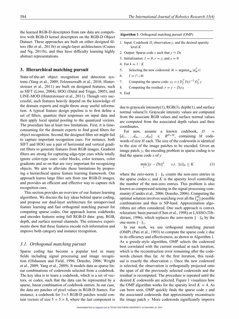
In our work, we use orthogonal matching pursuit(OMP) (Pati et al., 1993) to compute the sparse code x dueto its efficiency and effectiveness, as shown in Algorithm 1.As a greedy-style algorithm, OMP selects the codewordbest correlated with the current residual at each iteration,which is the reconstruction error remaining after the code-words chosen thus far. At the first iteration, this resid-ual is exactly the observation y. Once the new codewordis selected, the observation is orthogonally projected ontothe span of all the previously selected codewords and theresidual is recomputed. The procedure is repeated until thedesired K codewords are selected. Figure 1 visualizes howthe OMP algorithm works for the sparsity level K = 4. Ascan been seen, OMP quickly finds the sparse code x andthe associated codewords that approximately reconstructsthe image patch y. More codewords significantly improve



Bo et al. 585

Fig. 1. Visualization of orthogonal matching pursuit. From the leftmost column to the rightmost column: an image patch, residualfrom zero, one, two and three codewords (from top to bottom), reconstructions from one, two, three and four codewords, the selectedcodewords at the first, second, third and fourth iterations, the learned codebook on the RGB channel and the computed sparse code.

the quality of reconstructions. When four codewords areselected, the reconstructed image patch is almost identicalto the original one.

Figure 2 shows an example of an RGB-D image pairalong with reconstructions achieved for different levels ofsparsity. The shown results are achieved by non-overlapping5×5 reconstructed patches based on the learned codebooksvisualized in Figure 3, below. As can been seen, a sparsitylevel of K = 5 achieves results that are almost indistin-guishable from the input data, indicating that this techniquecould also be used for RGB-D compression (Ruhnke et al.,2013), contrary to Ruhnke et al. (2010). For object recog-nition, the sparse codes become the features representingimages, or patches.

The major advantages of OMP are its speed and its easeof implementation. Despite its simplicity, empirical evi-dence suggests that OMP works well in terms of approxima-tion performance (Tropp, 2004). In the past few years, therehas been significant interest in theoretical analysis of theOMP algorithm (Tropp and Gilbert, 2007; Jain et al., 2011;Zhang, 2011). Tropp and Gilbert (2007) demonstrated the-oretically and empirically that OMP can recover a signalwith K nonzero entries in dimension M with large proba-bility, given O( K ln M) random linear measurements of thatsignal. Zhang (2011) commented that basis pursuit (Chenet al., 1998), i.e. a one-norm based convex optimizationapproach, is slightly more favorable in terms of its depen-dency on the lower strong convexity constant, while OMPis more favorable in terms of its dependency on the upperstrong convexity constant. Since the OMP algorithm isfaster and easier to implement, it is an attractive alterna-tive to convex relaxation approaches for image recoveryproblems.

Recently, more and more attention has been focused onstudying OMP under the restricted isometry property (Dav-enport and Wakin, 2010; Livshitz, 2010; Jain et al., 2011;Mo and Shen, 2012). To see, let δK+1 be the restricted isom-etry constant of the measurement matrix (here codebook).Davenport and Wakin (2010) proved that δK+1 < 1

3√

Kis

sufficient for OMP to uniformly recover any K-sparse signalin K iterations. Mo and Shen (2012) further improved theabove sufficient condition and showed that δK+1 < 1√

K+1is

sufficient for OMP to recover any K-sparse vector in K iter-ations. Both above results require O( K2) measurements forthe recovery of a K-sparse vector. Livshitz (2010) provedthat K-sparse vectors can be recovered via OMP by essen-tially a lesser number of measurements O( K1.6 ln M). Theresults are strong from the theoretical viewpoint and pro-vide an explanation why OMP works well in practice. In ourcase, K is much smaller than the number of measurementsH and OMP is expected to find a good solution.

In our HMP, OMP is used to efficiently compute thesparse codes for image patches at the first layer and pooledsparse codes at the second layer. In our setting, a large num-ber of image patches share the same codebook and the totalcomputational cost of OMP can be reduced by a batch ver-sion that keeps some quantities in memory (Davis et al.,1997; Rubinstein et al., 2008; Bo et al., 2011c). We analyzethe batch versions of OMP in details in Section 3.4. We firstturn out attention to learning codebooks from image data.

3.2. Codebook learning via K-SVD

K-SVD (Aharon et al., 2006) is a popular codebook learn-ing approach that learns an overcomplete codebook from aset of observations with sparsity constraints. The approachhas lead to the state-of-the-art results in various applica-tions such as image denoising (Elad and Aharon, 2006b),face image compression (Bryt and Elad, 2008), texturesegmentation (Mairal et al., 2008a), and contour detec-tion (Ren and Bo, 2012). K-SVD learns codebooks D =[d1, . . . , dm, . . . , dM ] ∈ RH×M and the associated sparsecodes X = [x1, . . . , xn, . . . , xN ] ∈ RM×N from a matrixY = [y1, . . . , yn, . . . , yN ] ∈ RH×N of observed data byminimizing the overall reconstruction error

minD,X

‖Y − DX‖2F s.t. ∀m, ‖dm‖2 = 1 and ∀n, ‖xn‖0 ≤ K

(2)




Fig. 2. Reconstructed images using the learned codebooks. Left: Original RGB and depth images. Middle: Reconstructed RGB anddepth images using only two codewords per 5 × 5 patch. Right: Reconstructions using five codewords.

Algorithm 2: Codebook learning via K-SVD

1. Input: Data matrix Y , and the desired sparsity level K

2. Output: Codebook D

3. Initialize the codebook D with Discrete Cosine Dictionary

4. Alternate between

5. Computing sparse codes using OMP and the current

codebook D

6. Updating codebook D via SVD based on computed

sparse codes

7. End

Here, N is the size of the training data, the notation ‖A‖F

denotes the Frobenius norm, the zero-norm ‖ · ‖0 counts thenon-zero entries in the sparse codes xn, and K is the sparsitylevel controlling the number of non-zero entries. When thesparsity level is set to 1 and the sparse code matrix is forcedto be a binary(0/1) matrix, K-SVD exactly reproduces thek-means algorithm.

K-SVD solves the optimization problem (2) in an alter-nating manner as outlined in Algorithm 2. During eachiteration, the current codebook D is used to encode the dataY by computing the sparse code matrix X . Then, the code-words of the codebook are updated one at a time, resultingin a new codebook. This new codebook is then used in thenext iteration to recompute the sparse code matrix followedby another round of codebook update.

Computing the sparse code matrix via orthogonalmatching pursuit: Given the current codebook D, optimiz-ing the sparse code matrix X is decoupled into N encod-ing problems, i.e. equation (1); one for each data item y.Orthogonal matching pursuit is used to compute the sparsecode x of y, as discussed in Section 3.1.

Updating the codebook via singular value decomposi-tion: Given the sparse code matrix X , the codebook D

Fig. 3. Codebooks learned for different channels. From left toright: Grayscale intensity, RGB, depth, 3D surface normal (threenormal dimensions color coded as RGB). The codeword sizes are5 × 5 × 1 for grayscale intensity and depth values, and 5 × 5 × 3for RGB and surface normal values. Codebook sizes are 75 forgrayscale intensity and depth values, and 150 for RGB and surfacenormal values.

is optimized sequentially via singular value decomposition(SVD). In the mth step, the mth codeword and its sparsecodes can be computed by performing SVD of the residualmatrix corresponding to that codeword

‖Y − DX‖2F = ‖Y −

∑i�=m

dix�i − dmx�

m‖2F = ‖Rm − dmx�

m‖2F

(3)

where x�i are the rows of X , and Rm = Y −∑

i�=m dix�i is the

residual matrix for the mth codeword. This matrix containsthe differences between the observations and their approxi-mations using all other codewords and their sparse codes.To avoid introducing new non-zero entries in the sparsecode matrix X , the update process only considers obser-vations that use the mth codeword. It can be shown thateach iteration of codebook learning followed by codebookupdating decreases the reconstruction error (2). In practice,K-SVD converges to good codebooks for a wide range ofinitializations (Aharon et al., 2006).



Bo et al. 587

In our HMP, K-SVD is used to learn codebooks at twolayers, where the data matrix Y in the first layer consistsof patches sampled from RGB-D images, and Y in thesecond layer are sparse codes pooled from the first layer(details below). Figure 3 visualizes the learned codebooksin the first layer for four channels: grayscale and RGBfor RGB images, and depth and surface normal for depthimages. As can been seen, the learned codebooks have veryrich appearances and include separated red, green, and bluecolors, transition filters between different colors, gray andcolor edges, gray and color texture filters, depth and nor-mal edges, depth center-surround (dot) filters, flat normals,and so on, suggesting many recognition cues of raw data arewell captured.

It is helpful to consider both RGB and grayscale channelssince our codebooks are learned in a hierarchical manner.In the first layer, the codebook learned on the RGB channelcontains the most recognition cues captured by the code-book learned on the grayscale channel. However, in thesecond layer, each codeword learned on the RGB channelincludes both color and non-color recognition cues whilethe one learned on the grayscale channel only includesnon-color recognition cues. This leads to complementaryfeatures and boosts the recognition accuracy significantly,particularly for category recognition, which will be furtherdemonstrated in the experiments.

We treat the sparsity level K, the codebook size N , andthe codeword dimensionality H (uniquely determined bythe patch size given the codebook size) as hyperparametersand search for them by ten-fold cross validation on trainingdata. In the experiments, we show how category recogni-tion changes with the sparsity level and the patch size inFigure 9, below. We found that the recognition accuracy isquite robust to these parameters and a set of fixed valuesseem to work well on different benchmarks.

3.3. Architecture of hierarchical matchingpursuit

In object recognition, images are frequently modeled asunordered collections of local patches, i.e. bag of patches.Such models are flexible, and the image itself can be con-sidered as a special case (bag with one large patch). Tra-ditional bag-of-patches models introduce invariance whilecompletely ignoring spatial information of patches that isgenerally useful for visual recognition. Spatial pyramidbag-of-patches models (Lazebnik et al., 2006) overcomethe above problem by organizing patches into spatial cellsat multiple levels (pyramid) and then concatenating fea-tures from spatial cells into one feature vector. Such mod-els effectively balance the importance of invariance anddiscriminative power, leading to much better performancethan simple bags. Spatial pyramid modeling is a compellingstrategy for unsupervised feature learning, because of anumber of advantages: (1) bag-of-patches virtually generatea large number of training samples (patches) for learning

algorithms and decrease the chance of overfitting; (2) localinvariance and stability of the learned features are increasedby pooling features in spatial cells.

Hierarchical matching pursuit builds feature hierarchiesby applying the orthogonal matching pursuit encoder recur-sively (Figure 4). The encoder consists of three modules:orthogonal matching pursuit, spatial pyramid max pooling,and contrast normalization. To balance invariance and spa-tial information, we aggregate sparse codes at each layerby spatial pyramid max pooling followed by contrast nor-malization. Our approach can be viewed as a dual-layerspatial pyramid bag-of-patches model where patches arerepresented as sparse codes. In the following, we discussa dual-layer HMP network in detail.

First layer: The goal of the first layer is to generate pooledsparse codes (features) for image patches whose size is typ-ically 16 × 16 pixels or larger. Each pixel in such a patchis represented by the sparse codes computed from a smallneighborhood around this pixel (for instance, 5 × 5 pixelregion). Spatial pyramid max pooling is then applied tothese sparse codes to generate patch level features. Spa-tial pyramid max pooling partitions an image patch P intomultiple level spatial cells. The features of each spatial cellC are the max pooled sparse codes, which are simply thecomponent-wise maxima over all sparse codes within a cell:

F( C) =[

maxj∈C

|xj1|, . . . , maxj∈C

|xjm|, . . . , maxj∈C

|xjM |]

(4)

Here, j ranges over all entries in the cell, and xjm is the mthcomponent of the sparse code vector xj of entry j. Note thatF( C) has the same dimensionality as the original sparsecodes but may be less sparse due to the max pooling opera-tion. The feature FP describing a 16×16 image patch P arethe concatenation of aggregated sparse codes in each spatialcell

FP = [F( CP

1 ) , . . . , F( CPs ) , . . . , F( CP

S )]

(5)

where CPs ⊆ P is a spatial cell generated by spatial pyra-

mid partitions over the image patches, and S is the totalnumber of spatial cells. As an example, we visualize spatialcells generated by a three-level spatial pyramid pooling ona 16×16 image patch in Figure 5: 4×4, 2×2, and 1×1 cellsizes. In this example, the dimensionality of the pooled fea-ture vector FP is ( 16 + 4 + 1) M , where M is the size of thecodebook (see also Figure 4). The main idea behind spatialpyramid pooling is to allow the features FP to encode dif-ferent levels of invariance to local deformations (Lee et al.,2009; Yang et al., 2009; Bo et al., 2011c), thereby increas-ing the discrimination of the features. An alternative way tocapture fine-grained cues is to use a multipath architecture,as recently investigated in Bo et al. (2013).

We additionally normalize the feature vectors FP by theirL2 norm

√‖FP‖2 + ε, where ε is a small positive number

to make sure the denominator is larger than zero. Since themagnitude of sparse codes varies over a wide range due to




Fig. 4. Hierarchical matching pursuit for RGB-D object recognition. In the first layer, sparse codes are computed on small patchesaround each pixel. These sparse codes are pooled into feature vectors representing 16 × 16 patches, by spatial pyramid max poolingand contrast normalization. The second layer encodes these feature vectors using orthogonal matching pursuit and codebooks learnedfrom sampled feature vectors. Whole image features are then generated from the resulting sparse codes, again by spatial pyramid maxpooling and contrast normalization.

Fig. 5. Spatial pyramid partitions over a 16 × 16 image patch. Each black dot denotes sparse codes of a pixel that are computed ona 5 × 5 small patch around this pixel using orthogonal matching pursuit. Left: Level 2. The 16 × 16 image patch is partitioned into4 × 4 = 16 spatial cells. Each cell is represented by the component-wise maximum of the sparse codes of pixels within the cell, F( C).Middle: Level 1. The 16 × 16 image patch is partitioned into 2 × 2 = 4 spatial cells. Right: Level 0. The whole 16 × 16 image patch isone spatial cell. The feature vector for the whole 16 × 16 image patch is the concatenation of C1 through C21.

local variations in illumination and occlusion, this opera-tion makes the appearance features robust to such varia-tions, as commonly done in the designed SIFT features.Contrast normalization often improves the recognitionaccuracy by about 2%. Our experiments suggest that asmall but non-negligible ε = 0.1 works best for the firstlayer and leads to about 1% improvement over a negligibleε = 0.0001.

Second layer: The goal of the second layer in HMPis to generate features for a whole image/object. To doso, HMP applies the sparse coding and max poolingsteps to image patch features FP generated in the firstlayer. The codebook for this level is learned by sam-pling patch features FP over RGB-D images. To extractthe feature describing a whole image, HMP first computespatch features via the first layer (usually, these patchescover 16 × 16 pixels and are sampled with a step sizeof 4 × 4 pixels). Then, just as in the first layer, sparsecodes of each image patch are computed using orthog-onal matching pursuit, followed by spatial pyramid maxpooling and contrast normalization (Figure 6). In this layer,however, we perform max pooling over both the sparse

Fig. 6. Spatial pyramid partitions over the whole image. Left:Level 2. The whole image is partitioned into 3 × 3 = 9 spatialcells. Each cell is represented by the component-wise maximumof the sparse codes of 16 × 16 patches within the cell, F( C). Mid-dle: Level 1. The whole image is partitioned into 2×2 = 4 spatialcells. Right: Level 0. The whole image is one spatial cell. Thefeature vector for the whole image is the concatenation of pooledsparse codes over C1 through C14.

codes and the patch level features computed in the firstlayer:

F( C) =[

maxj∈C

|zj1|, . . . , maxj∈C

|zjU |, maxj∈C

|Fj1|, . . . , maxj∈C

|FjV |]

(6)



Bo et al. 589

Here, C is a cell and Fj and zj are the patch features and theirsparse codes, respectively. U and V are the dimensionalityof zj and Fj, where U is given by the size of the layer twocodebook, and V is given by the size of the patch level fea-ture computed via (5). Jointly pooling zj and Fj integratesboth fine-grained cues captured by the codewords in the firstlayer and coarse-grained cues by those in the second layer,increasing the discrimination of the features.

The features of the whole image/object are the concate-nation of the aggregated sparse codes within each spatialcell

FI = [F( CP

1 ) , . . . , F( CPs ) , . . . , F( CP

S )]

(7)

where CPs ⊆ P is a spatial cell generated by spatial pyramid

partitions over the whole image, and S is the total numberof spatial cells. The image feature vector FI is then normal-ized by dividing with its L2 norm

√‖FI‖2 + 0.0001. In the

higher layers, we use a negligible ε = 0.0001: a larger valuedecreases the accuracy but a smaller one works as well asε = 0.0001.

Though we only consider two layers in this paper, itis straightforward to append more layers in a similarway to generate deep representations. The features fromdifferent layers encode different amounts of spatial invari-ance (mainly due to spatial pooling and contrast normaliza-tion), so additional layers could boost the accuracy further,as shown in Bo et al. (2013). It should be noted thatHMP is a fully unsupervised feature learning approach:no supervision (e.g. object class) is required for code-book learning and feature coding. The feature vectors FI

of images/objects and their corresponding labels are thenfed to classifiers to learn recognition models.

3.4. Fast orthogonal matching pursuit

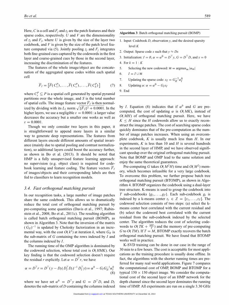
In our recognition tasks, a large number of image patchesshare the same codebook. This allows us to dramaticallyreduce the total cost of orthogonal matching pursuit bypre-computing some quantities (Davis et al., 1997; Rubin-stein et al., 2008; Bo et al., 2011c). The resulting algorithmis called batch orthogonal matching pursuit (BOMP), asshown in Algorithm 3. Note that the inversion of the matrix( GII )−1 is updated by Cholesky factorization in an incre-mental way, with the cost O( k2) at iteration k, where GII isthe sub-matrix of G containing the rows indexed by I andthe columns indexed by I .

The running time of the OMP algorithm is dominated bythe codeword selection, whose total cost is O( HMK). Ourkey finding is that the codeword selection doesn’t requirethe residual r explicitly. Let α = D�r, we have

α = D�r = D�( y − DI ( D�I DI )

−1 D�I y) = α0 − GI G

−1II α0

I(8)

where we have set α0 = D�y and G = D�D, and DI

denotes the sub-matrix of D containing the columns indexed

Algorithm 3: Batch orthogonal matching pursuit (BOMP)

1. Input: Codebook D, observation y, and the desired sparsity

level K


3. Initialization: I = ∅, α = α0 = D�y, G = D�D, and x = 0

4. For k = 1 : K

5. Selecting the new codeword: m = argmaxm |αm|6. I = I ∪ m

7. Updating the sparse code: xI = G−1II α0

I

8. Updating α: α = α0 − GI xI

9. End

by I . Equation (8) indicates that if α0 and G are pre-computed, the cost of updating α is O( MK), instead ofO( MH) of orthogonal matching pursuit. Here, we haveK ≤ H since the H codewords allow us to exactly recon-struct the image patches. The cost of searching sparse codesquickly dominates that of the pre-computation as the num-ber of image patches increases. When using an overcom-plete codebook, K is usually much less than H . In ourexperiments, K is less than 10 and H is several hundredsin the second layer of HMP, and we have observed signifi-cant speedup over the original orthogonal matching pursuit.Note that BOMP and OMP lead to the same solution andenjoy the same theoretical guarantees.

Pre-computing G takes O( M2H) time and O( M2) mem-ory, which becomes infeasible for a very large codebook.To overcome this problem, we further propose batch treeorthogonal matching pursuit (BTOMP), as shown in Algo-rithm 4. BTOMP organizes the codebook using a dual-layertree structure. K-means is used to group the codebook intoT sub-codebooks {g1, . . . , gT }. Each sub-codebook gt isindexed by a k-means center zt ∈ Z = [z1, . . . , zT ]. Thecodeword selection consists of two steps: (a) select the k-means center best correlated with the current residual and(b) select the codeword best correlated with the currentresidual from the sub-codebook indexed by the selectedcenter. The algorithm reduces the cost of selecting code-words to O( TK + MH

T ) and the memory of pre-computingG to O( TM). If T = M , BTOMP exactly recovers the batchorthogonal matching pursuit. We have found that BTOMPworks well in practice.

K-SVD training can be done in our case in the range of30 min to a few hours. The cost is acceptable for most appli-cations as the training procedure is usually done offline. Infact, the algorithms with the shorter running times are pre-ferred for many real world applications. Figure 7 comparesthe computational cost of OMP, BOMP and BTOMP for atypical 150 × 150 object image. We consider the computa-tional cost of the second layer of an HMP network for thedepth channel since the second layer dominates the runningtime of HMP. All experiments are run on a single 3.30 GHz




Algorithm 4: Batch tree orthogonal matching pursuit (BTOMP)

1. Input: Codebook D, Centers Z, observation y, and sparsity

level K


3. Initialization: I = ∅, r = y, α = α0 = Z�y, B = Z�D,

and x = 0

4. For k = 1 : K

5. Choosing the sub-codebook gt: t = argmaxt |αt|6. Selecting the new codeword: m = argmaxm∈gt

|d�m r|

7. I = I ∪ m

8. Updating the sparse code: xI = ( D�I DI )−1 D�

I y

9. Updating α: α = α0 − BI xI

10. Computing the residual: r = y − DI xI

11. End

Fig. 7. Computational cost of OMP, BOMP and BTOMP. Left:1000 codewords are used for comparisons. Right: 10,000 code-words are used for comparisons.

Intel Xeon CPU with a single thread. As can been seen fromthe left of Figure 7, BOMP takes about 0.3 s to computesparse codes and is much faster than the flat OMP. For com-parisons, we also run the efficient feature-sign search algo-rithm (Lee et al., 2006) to compute sparse codes from theL1 based convex optimization. The procedure takes about15 s under the comparable sparsity constraint with K = 10,significantly slower than BOMP. As can been seen from theright of Figure 7, BTOMP is more than three times fasterthan BOMP for larger codebooks. Our experiments suggestthat BTOMP provides virtually the same performance asBOMP.

4. Experiments

We evaluate our RGB-D HMP framework on three publiclyavailable RGB-D object recognition datasets and two RGBobject recognition datasets. We compare HMP to resultsachieved by state-of-the-art algorithms published with thesedatasets. For all five datasets, we follow the same trainingand test procedures used by the corresponding authors ontheir respective data. All images are resized to be no largerthan 300 × 300 pixels with preserved ratio.

In the first layer, we learn dictionaries of size 75 withsparsity level 5 on 1,000,000 sampled 5 × 5 raw patches forgrayscale and depth channels, and codebooks of size 150 on1,000,000 sampled 5 × 5 × 3 raw patches for RGB and nor-mal channels using K-SVD. We remove the zero frequencycomponent from raw patches by subtracting their mean andinitialize K-SVD with overcomplete dictionaries generatedby the Discrete Cosine Transform (Bo et al., 2011c). Ascan be seen from Figure 3, the learned codebooks over fourchannels capture a large variety of distinguishable struc-tures from raw pixels. With the learned codebooks, wecompute sparse codes of each pixel (5 × 5 patch aroundit) using batch OMP with sparsity level 5, and generatepatch level features by max pooling over 16 × 16 imagepatches with 4×4, 2×2, and 1×1 partitions. The resultingpatch level features are 21 × 75 = 1575-dimensional vec-tors or 21 × 150 = 3150-dimensional vectors. Note thatthis architecture leads to fast computation of patch levelfeatures.

In the second layer, we learn codebooks of size 1000with sparsity level 10 on pooled sparse codes sampledover 1,000,000 16 × 16 patches for each of four channelsusing K-SVD. We initialize K-SVD with randomly sampledpooled sparse codes (Bo et al., 2011c). With the learnedcodebooks, we compute sparse codes of image patches thatare densely sampled from the whole image with a step sizeof 4 × 4 pixels. We then pool both patch level features andtheir sparse codes on the whole image with 3×3, 2×2, and1 × 1 partitions to generate the image level features. Thefinal image feature vectors are the concatenation of thosefrom all four channels, resulting in a feature size of 188,300dimensions.

The above hyperparameters are optimized on a subsetof the RGB-D object recognition dataset we collected. Weempirically found that they work well on different datasets.In the following experiments, we will keep these values ofparameters fixed, even though it might further improve theaccuracy via tuning these parameters per dataset using crossvalidation on the associated training data. With the learnedHMP features, linear support vector machines (SVMs) aretrained for recognition. For comparisons, we have experi-mented with linear logistic regression classifiers, and foundthat it is consistently worse than linear SVMs by about2%. Linear SVMs are able to match the performance ofnonlinear SVMs with the popular histogram intersectionkernel (Maji et al., 2008) while being scalable to largedatasets (Bo et al., 2011c).

4.1. RGB-D object dataset

The first dataset, called RGBD, contains 41,877 RGB-Dimages of 300 everyday objects taken from different view-points (Lai et al., 2011a). The objects are organized into51 categories arranged using WordNet hypernym–hyponymrelationships. The objects in the dataset are segmented fromthe background by combining color and depth segmenta-tion cues. The RGBD dataset is challenging since it not



Bo et al. 591

Fig. 8. Category recognition accuracy with different channels anddifferent layers using depth images only. Depth_1 and Depth_2denote single-layer and dual-layer HMP networks for the depthchannel, respectively. Normal_1 and Normal_2 denote single-layer and dual-layer HMP networks for the surface normal chan-nel, respectively. Depth_1+2 and Normal_1+2 denote the combi-nation of the single-layer and the dual-layer HMP networks for thedepth and the surface normal channels, respectively. “All” denotesthe combination of all HMP networks.

Fig. 9. Category recognition accuracy with different sparsity lev-els and different patch sizes. Left: Category recognition accuracyas a function of sparsity level in the second layer of HMP for thedepth and surface normal channels, respectively. Right: Categoryrecognition accuracy as a function of patch size in the second layerof HMP.

only contains textured objects such as food bags, sodacans, and cereal boxes, but also texture-less objects suchas bowls, coffee mugs, fruits, or vegetables. In addition,the data frames in RGBD exhibit large changes in lightingconditions.

We distinguish between two types of object recognitiontasks: category recognition and instance recognition. Cat-egory recognition is to determine the category name of apreviously unseen object. Each object category consists ofa number of different object instances. Instance recognitionis to recognize known object instances. Following the exper-imental setting in Lai et al. (2011a), we randomly leaveone object instance out from each category for testing, andtrain models on the remaining 300 − 51 = 249 objectsat each trial for category recognition. We report the accu-racy averaged over 10 random train/test splits. For instancerecognition, we train models on images captured from 30◦

and 60◦ elevation angles, and test them on the images of the45◦ angle (leave-sequence-out).

4.1.1. Object recognition using depth images. To providea better understanding of our approach, we performed a

detailed analysis of architecture and hyperparameters ofHMP on depth images. We chose the depth channel becauseless attention has been paid to it in the deep learningcommunity. In fact, similar conclusions hold for the colorchannel.

Though the deep learning community emphasized thatmulti-layer architectures are necessary for maximizing theaccuracy, Coates and Ng (2011b) provide counterintuitiveevidence by showing that single-layer networks work aswell as multi-layer networks for object recognition ondatasets they used. However, more recent work (Hintonet al., 2012; Le et al., 2012) shows that deep architec-tures trained on large-scale datasets significantly outper-form single-layer networks and lead to large improvementsover the state-of-the-art. This indicates that a large amountof training data might be the key to the success of deepnetworks.

To demonstrate that multi-layer HMP networks helpRGB-D object recognition, we perform the experiments forcategory recognition with both single-layer and dual-layerHMP networks on the depth and surface normal channels.The results are reported in Figure 8. First of all, we observethat dual-layer HMP networks are always better than single-layer HMP networks: about 9% higher on the depth channeland about 1% higher on the surface normal channel. Thecombination of the single-layer and the dual-layer HMPnetworks outperform either one and further boosts the accu-racy. The combination of all HMP networks achieves thehighest recognition accuracy, significantly better than thebest single HMP network.

These results are very encouraging and provide strongevidence for the importance of architectures of multiplechannels and multiple layers. We believe that features fromdifferent layers provide complementary information that isthe key for their success. Intuitively, features from the firstlayer capture basic structures of patches and are sensitiveto spatial displacement. Features from the second layer arehighly abstract, and robust to local deformations due to theintroduction of spatial max pooling and contrast normaliza-tion in the first layer. These features are strong in their ownright and their combination turns out to be much better thanthe best single one.

The sparsity level K and the patch size should be selectedcarefully to maximize the performance of HMP. A smallK might lead to poor approximation and discard too muchuseful information, while an overly large K increases thecomputational cost and the risk of overfitting to unnecessarydetails. On the other hand, it is difficult to capture sufficientspatial context with a small patch size while an overly largepatch size could incur severe over-smoothing on importantstructures.

To understand the influence of these parameters, wevary the sparsity level and the patch size while fixing allother parameters to default values. We report the results inFigure 9. As can been seen, both small and large K valuesdecrease accuracy, and the best test accuracy is achieved




when K is around 10. The test accuracy becomes saturatedwhen the patch size is larger than a threshold (here 5). Thepatch size of 5 gives the highest test accuracy among allpatch sizes.

Spatial pyramid max pooling enables different levels ofspatial context, and outperforms flat spatial max pooling(3 × 3 partitions) by about 2% in our experiments. Weperformed HMP with and without contrast normalizationand found that contrast normalization improves recognitionaccuracy by about 3%, which indicates the importance ofthis component for learning robust features.

4.1.2. Object recognition using both RGB and depthimages. We compare HMP with the baseline (Lai et al.,2011a), fast point feature histograms (Aldoma et al., 2012),kernel descriptors (Bo et al., 2011b), and convolutionalk-means descriptors (CKM Desc) (Blum et al., 2012) inTable 1. Fast point feature histograms capture the relativeorientation of normals, as well as distances, between pointpairs. Note that these descriptors are standard features for3D point clouds in the 3D point cloud library (Aldomaet al., 2012). Convolutional k-means descriptors adaptthe k-means based feature learning approach proposed byCoates and Ng (2011b) to the RGB-D setting. The recog-nition systems developed in Lai et al. (2011a), Bo et al.(2011b), and Lai et al. (2012b) use a rich set of manu-ally designed features. As can been seen, HMP outperformsall previous approaches for both category and instancerecognition.

We performed additional experiments to shed light ondifferent aspects of our approach for instance recognition.In Figure 10 (left), we show instance recognition accu-racy using features on grayscale images and features oncolor images, and both. As can been seen, features on colorimages work much better than those on grayscale images.This is expected since color information plays an importantrole for instance recognition. Object instances that are dis-tinctive in the color space may have very similar appearancein grayscale space. We investigated the object instancesmisclassified by HMP, and found that most of the mistakesare from fruits and vegetables. Two misclassified tomatoesare shown in Figure 10. As one can see, these two tomatoinstances are so similar that even humans struggle to tellthem apart. If such objects are excluded from the dataset,our approach has more than 95% accuracy for instancerecognition on the RGBD dataset.

4.1.3. Pose estimation. We further evaluated the HMP fea-tures for pose estimation, where the pose of every viewof every object is annotated as the angle about the verti-cal axis. Each object category has a canonical pose that islabeled as 0◦, and every image in the dataset is labeled witha pose in [0, 360◦]. Similar to instance recognition, we usethe 30◦ and 60◦ viewing angle sequences as training dataand the 45◦ sequence as test set. For efficiency, we followan independent tree approach to estimate pose, where each

Fig. 10. Left: Instance recognition accuracy by using features ongrayscale images (Gray), features on color images (RGB), andboth (Gray + RGB). Right: Two tomato instances confused by ourapproach.

level is trained as an independent classier (Lai et al., 2011b).Firstly, one-versus-all category classifiers are trained in thecategory level; secondly, one-versus-all instance classifiersare trained in the instance level within each category; andfinally one-versus-all pose classifiers in the pose level aretrained within each instance. At test time, category, instanceand pose classifiers are run in turn to estimate the pose of aquery object.

Table 2 shows pose estimation errors under three differ-ent scenarios. We report both median pose (MedPose) andmean pose (AvePose) errors because the distribution acrossobjects is skewed (Lai et al., 2011b). For MedPose andAvePose, pose errors are computed on the entire test set,where test images that were assigned an incorrect categoryor instance label have a pose error of 180.0◦. MedPose(C)and AvePose(C) are computed only on test images that wereassigned the correct category by the system, and, Med-Pose(I) and AvePose(I) are computed only on test imagesthat were assigned the correct instance by the system. Wecompare HMP to our previous results (Lai et al., 2011b).As can been seen from Table 2, with our new HMP fea-tures, pose estimation errors are significantly reduced underall scenarios, resulting in only 20◦ median error even whenclassification errors are measured as 180.0◦ offset. We visu-alize test images and the best matched images in Figure 11.The results are very intuitive: estimations are quite accu-rate for non-symmetric objects and sometimes inaccuratefor symmetric objects for which different poses could sharevery similar or the same appearances.

4.1.4. Hierarchical segmentation based object detection.So far, our evaluation focused on object recognition, inwhich the object of interest occupies major portions of animage, or image segment. This setting applies, for instance,to robot manipulation tasks in which objects can easilybe segmented from a scene, such as objects placed suffi-ciently far from each other on a table top. However, in manyrobotics tasks the location, or even presence, of an objectis not known in advance and the object might be partiallyoccluded by other objects. This is the more challengingobject detection problem.



Bo et al. 593

Table 1. Comparisons with the baseline (Lai et al., 2011a), fast point feature histograms (Aldoma et al., 2012), kernel descriptors (Boet al., 2011b), and convolutional k-means descriptor (Blum et al., 2012).

RGBD Category InstanceMethods RGB Depth RGB-D RGB Depth RGB-D

ICRA11 (Lai et al., 2011a) 74.3 ± 3.3 53.1 ± 1.7 81.9 ± 2.8 59.3 32.3 73.9FPFH (Aldoma et al., 2012) / 56.0 ± 1.5 / / / /CKM Desc (Blum et al., 2012) / / 86.4 ± 2.3 82.9 / 90.4Kernel descriptors (Bo et al., 2011b; Lai et al., 2012b) 80.7 ± 2.1 80.3 ± 2.9 86.5 ± 2.1 90.8 54.7 91.2HMP 82.4 ± 3.1 81.2 ± 2.3 87.5 ± 2.9 92.1 51.7 92.8

Table 2. Pose estimation error (in degrees) and running time (in seconds) comparison against several approaches using kernel descrip-tors as features. Indep Tree is a tree of classifiers where each level is trained as independent linear SVMs, NN is nearest neighborregressor, and OPTree is the Object-Pose Tree proposed in Lai et al. (2011b). Median pose accuracies for MedPose, MedPose(C), andMedPose(I) are 88.9%, 89.6%, and 90.0%, respectively. Mean pose accuracies for AvePose, AvePose(C), and AvePose(I) are 70.2%,73.6%, and 75.1%, respectively.

Technique MedPose (◦) MedPose(C) (◦) MedPose(I) (◦) AvePose (◦) AvePose(C) (◦) AvePose(I) (◦) Test time (s)

NN 144.0 105.1 33.5 109.6 98.8 62.6 54.8Indep Tree 73.3 62.1 44.6 89.3 81.4 63.0 0.31OPTree 62.6 51.5 30.2 83.7 77.7 57.1 0.33HMP 20.0 18.7 18.0 53.6 47.5 44.8 0.51

Fig. 11. Test images and the best matched angles in the training data using HMP features.

In this section we demonstrate the applicability of ourhierarchical feature learning approach to object detection.The classical object detection pipeline is based on brute-force, for instance, sliding window approaches. By extract-ing fixed-size image rectangles at multiple locations andscales, sliding window approaches reduce object detectionto a binary classification problem, i.e. “is the image rectan-gle an object or background?” Here, we consider an alter-native segmentation based detection pipeline in order tofully leverage the strengths of depth information. Recentresearch along this line has achieved impressive resultsin the PASCAL VOC detection and segmentation chal-lenge (Van de Sande et al., 2011; Carreira et al., 2012)and RGB-D scene labeling (Ren et al., 2012). Instead of

classifying image rectangles, segmentation based detec-tion approaches classify the segments generated by a seg-mentation algorithm into object or background segments.The pipeline is particularly interesting for us since depthinformation is available and it makes segmentation mucheasier.

To generate segments from an RGB-D scene, we followcontour based segmentation approaches (Arbelaez et al.,2011): first, detect contours of the scene and then con-vert them into a hierarchical segment tree. We use recentlyintroduced sparse code gradients (SCG) for contour detec-tion due to its proven performance and ability to deal withRGB-D images (Ren and Bo, 2012). SCG applies K-SVDto learn dictionaries on RGB and depth channels and then




Fig. 12. Segmentation Results. Top-left: Original RGB image. Top-middle: SCG contours. Both RGB and depth channels are used.Top-right: Ultrametric contour map (UCM) generated from SCG contours. Bottom Segment map generated by thresholding UCM atthree different levels. Different segments are shown in different colors.

uses OMP to encode rich contour cues by computing sparsecodes on oriented local neighborhoods in multiple scalesand pooling them together. SCG provides an elegant wayto measure local contrasts and improves the previous bestcontour detection algorithm, global probability of bound-ary (gPb) (Arbelaez et al., 2011) by a large margin (Renand Bo, 2012).

We extract hierarchical segments from an ultrametriccontour map (UCM) (Arbelaez et al., 2011) converted fromSCG contours. UCM defines a duality between closed,non-self intersecting weighted contours and a hierarchy ofregions, and its values reflect the contrast between neigh-boring regions. The hierarchy is constructed by a greedy,graph-based region merging algorithm, and segments at dif-ferent scales can be retrieved by thresholding the UCM atdifferent levels. Such nested collection of segments allowsobject classifiers to select the object segments from multi-ple levels and dramatically increases the accuracy of objectdetection.

We visualize SCG contours, SCG UCM, and the seg-ments at different levels on an RGB-D frame from theRGB-D Table Scene (Lai et al., 2011a) in Figure 12. Ascan been seen, SCG successfully detects most contours inthe scene, which again demonstrates the effectiveness ofsparse code features. Contour detection is quite challeng-ing in this scene due to complex lighting conditions andobject shadows. Depth information plays an important rolein good performance. SCG UCM are a collection of closedweighted contours, as shown in the middle of Figure 12. Thesegments inferred from SCG UCM are shown in the bot-tom of Figure 12. We observe that different objects preferdifferent scale levels. For instance, the segmentation in themiddle is best for the cereal box while the one in the right isbest for coffee mugs, suggesting the benefits of hierarchicalsegmentation.

For object detection, we compute HMP features overbounding boxes of segments of size at least 40 × 40 pixels.

Segments smaller than 24 × 24 pixels are not considered.All other segments are padded on each side of the segmentby 8 pixels to keep edge information. We then run a linearSVM for each object instance and classify the segments intoobjects or background. In addition to object instance class,we also include a background class consisting of the seg-ments generated from background scenes. Similarly to slid-ing window detection, we apply non-maximum suppressionto eliminate redundancy when multiple object segmentshave large spatial overlaps.

We evaluate our segmentation based object detection onthe RGB-D Table Scene, one of the most challenging scenesin Lai et al. (2011a). The whole video sequence consistsof 125 RGB-D frames and contains seven object instancesfrom five object categories: bowl, cap, cereal box, coffeemug and soda can. Note that flashlight, stapler and spraycan are considered as background for this task. We reportour object instance detection results in Figure 13. As canbeen seen, our approach gives not only the object bound-ing boxes (left) but also the object boundaries (middle).All target object instances are detected, except the highlyoccluded white cap (middle right). In the right of Figure 13,we show the precision-recall curves. Our average preci-sion is about 10 absolute% higher than the previous slidingwindow detectors (Lai et al., 2011a). The missing recall ismostly because the majority of objects are occluded or notcovered by a single segment.

This experiment demonstrates that HMP can be appliedsuccessfully to object detection, which is highly relevant tomany robot manipulation and perception tasks.

4.2. Willow and 2D3D datasets

We additionally evaluated HMP on two other pub-licly available RGB-D recognition datasets, without fur-ther tuning any of its parameters. The first dataset,2D3D, consists of 156 object instances organized into 14



Bo et al. 595

Fig. 13. Detection Results. Left: Detected object bounding boxes and their instance names. Middle: Detected object boundaries andtheir instance names. Note that flashlight, stapler and spray can are background for this task. Right: Precision-recall curves of our HMPdetector and the sliding window detector (Lai et al., 2011a).

categories (Browatzki et al., 2011). The authors of thisdataset use a large set of 2D and 3D manually designedshape and color features. SVMs are trained for each featureand object class, followed by multilayer perceptron learn-ing to combine the different features. The second dataset,Willow, contains objects from the Willow and Challengedatasets for training and testing, respectively (Tang et al.,2012) (Figure 14). Both training and test data contain 35rigid, textured, household objects captured from differentviews by Willow Garage. The authors present a processingpipeline that uses a combination of SIFT feature matchingand geometric verification to perform recognition of highlytextured object instances (Tang et al., 2012). Note that2D3D and Willow only contain highly textured objects.

We report the results of HMP in Table 3. Following theexperimental setting in Browatzki et al. (2011), HMP yields91.0% accuracy for category recognition, much higher thanthe 82.8% reported in Browatzki et al. (2011). Learningmodels on training data from the Willow dataset and testingthem on the training data from the Challenge dataset (Tanget al., 2012), HMP achieves higher precision/recall than thesystem proposed in (Tang et al., 2012), which won the 2011Perception Challenge organized by Willow Garage. Notethat this system is designed for textured objects and has notbeen evaluated on untextured objects such as those found inthe RGBD dataset.

4.3. Machine learning and vision datasets

In this section, we evaluate the HMP features on 2D imagesonly for object recognition and scene recognition tasks fre-quently considered in the machine learning and computervision communities. With the proposed dual-layer archi-tecture, HMP outperforms the state-of-the-art on standardlearning and vision benchmarks.

4.3.1. Object recognition STL-10. introduced by Coateset al. (2011) is a standard dataset for evaluating featurelearning approaches. We used the same architecture forthese datasets as for the RGB-D datasets. The codebooksare learned on both RGB and grayscale channels, and thefinal features are the concatenation of HMP features fromthese two channels. Following the standard setting in Coateset al. (2011), we train linear SVMs on 1000 images and test

on 8000 images using our HMP features and compute theaveraged accuracy over 10 folds pre-defined by the authors.

We report the results in Table 4. As can been seen,HMP achieves much higher accuracy than the receptivefield learning algorithm (Coates and Ng, 2011a) that beatsmany types of deep feature learning approaches as well assingle-layer sparse coding on top of SIFT (Coates and Ng,2011b). In addition, HMP outperforms discriminative sum-product networks (SPNs), a recently introduced deep learn-ing model (Gens and Domingos, 2012) that is trained in asupervised manner using an efficient backpropagation-stylealgorithm.

4.3.2. Scene recognition. Understanding scenes is animportant problem in robotics and has been a fundamentalresearch topic in computer vision for a while. We evaluateHMP on the popular MITScenes-67 dataset (Quattoniand Torralba, 2009). This dataset contains 15,620 imagesfrom 67 indoor scene categories. All images have a min-imum resolution of 200 pixels in each axis. Indoor scenerecognition is very challenging as the intra-class variationsare large and some scene categories are similar to oneanother. We used the same architecture for these datasetsas for RGB-D datasets. The codebooks are learned on bothRGB and grayscale channels and the final features are theconcatenation of HMP features from these two channels.

Following standard experimental setting (Pandey andLazebnik, 2011), we train models on 80 images andtest on 20 images per category on the pre-defined train-ing/test split by the authors. As can been seen in Table 5,HMP achieves higher accuracy than many state-of-the-artalgorithms: GIST (Quattoni and Torralba, 2009), SpatialPyramid Matching (SPM) (Pandey and Lazebnik, 2011),Deformable Parts Models (DPM) (Felzenszwalb et al.,2010), Object Bank (Li et al., 2010), Reconfigurable Mod-els (RBoW) (Parizi et al., 2012), and even the combinationof SPM, DPM, and color GIST (Pandey and Lazebnik,2011). The HMP features on both RGB and grayscale chan-nels achieve higher accuracy than those on either grayscalechannel only (41.8%) or RGB channel only (43.9%).

5. Conclusions

We have proposed HMP for learning multiple level sparsefeatures from raw RGB-D data. HMP learns codebooks




Fig. 14. Ten of the 35 textured household objects from the Willow dataset.

Table 3. Comparisons with the previous results on the two public datasets: Willow and 2D3D.

2D3D Category recognition Willow Instance recognition

Methods RGB Depth RGB-D Methods Precision/recallICCVWorkshop (Browatzki et al., 2011) 66.6 74.6 82.8 ICRA12 (Tang et al., 2012) 96.7/97.4HMP 86.3 87.6 91.0 HMP 97.4/100.0

Table 4. Comparisons with the previous results on STL-10.

MCML (Kiros andSzepesvri, 2012)

54.2 ± 0.4 Sparse Coding (Coatesand Ng, 2011b)

59.0 ± 0.8 SPNs (Gens andDomingos, 2012) 62.3

VQ (Coates et al.,2011)

54.9 ± 0.4 Learned RF (Coatesand Ng, 2011a)

60.1 ± 1.0 HMP 64.5 ± 1.0

Table 5. Comparisons with the previous results on MITScenes-67.

GIST (Quattoni andTorralba, 2009)

22.0 SPM (Pandey andLazebnik, 2011)

34.4 RBoW (Pariziet al., 2012)

37.9

GIST-color (Pandeyand Lazebnik, 2011)

29.7 Sparse Coding(Bo et al., 2011c)

36.9 DPM + Gist-color +SPM (Pandey andLazebnik, 2011)

43.1

DPM (Felzenszwalbet al., 2010)

30.4 Object Bank(Li et al., 2010)

37.6 HMP 47.6

at each layer via sparse coding on a large collection ofimage patches, or pooled sparse codes. With the learnedcodebooks, HMP builds feature hierarchies using orthog-onal matching pursuit, spatial pyramid pooling and con-trast normalization. We have proposed the batch versionsof orthogonal matching pursuit to significantly speed upthe computation of sparse codes at runtime. Our algo-rithms are scalable and can efficiently handle full-sizeRGB-D frames. HMP consistently outperforms state-of-the-art techniques on standard benchmark datasets. Theseresults are extremely encouraging, indicating that currentrecognition systems can be significantly improved with thelearned features.

We believe this work has the potential to significantlyimprove robotics capabilities in object recognition, targetedobject manipulation, and semantic scene understanding. Anextensive evaluation shows that HMP outperforms designedfeatures by a large margin for recognizing pre-segmentedobjects. Our experiments also show that HMP can sig-nificantly improve view-based pose estimation of objects,which has direct applications in robot grasping tasks. Theresults on object detection demonstrate furthermore that

HMP can be applied not only to pre-segmented objects, butalso to more general settings in which objects may occludeeach other and occupy only small fractions of a scene. HMPcan furthermore increase the capabilities of robots to under-stand commands given in natural language, since peopleoften refer to objects by their names and visual attributes,as recently investigated in Sun et al. (2013).

This work opens up many possibilities for learning rich,expressive features from raw RGB-D data. In the currentimplementation, we manually designed the architecture ofHMP. Automatically learning such structure is interestingbut also very challenging and left for future work. Ourcurrent experience is that learning dictionaries separatelyfor each channel works better than learning them jointly.We plan to explore other possibilities of joint dictionarylearning in the future.

Acknowledgments

This submission is an extension of our previous work presented atNIPS 2011 (Bo et al., 2011c) and ISER 2012 (Bo et al., 2012).



Bo et al. 597

Funding

This work was funded in part by the Intel Science and Technol-ogy Center for Pervasive Computing and by ONR MURI (grantnumber N00014-07-1-0749).

References

Aharon M, Elad M and Bruckstein A (2006) K-SVD: An algo-rithm for designing overcomplete dictionaries for sparse rep-resentation. IEEE Transactions on Signal Processing 54(11):4311–4322.

Aldoma A, Marton Z, Tombari F, et al. (2012) Tutorial: Pointcloud library: three-dimensional object recognition and 6 DOFpose estimation. IEEE Robotics and Automation Magazine 19:80–91.

Anand A, Koppula H, Joachims T, et al. (2012) Contextuallyguided semantic labeling and search for 3D point clouds.International Journal of Robotics Research 32(1): 19–34.

Arbelaez P, Maire M, Fowlkes C, et al. (2011) Contour detec-tion and hierarchical image segmentation. IEEE Transactionson Pattern Analysis and Machine Intelligence 33(5): 898–916.

Bay H, Ess A, Tuytelaars T, et al. (2008) Speeded-up robustfeatures (SURF). Computer Vision and Image Understanding110(3): 346–359.

Blum M, Springenberg J, Wülfing J and Riedmiller M (2012)A learned feature descriptor for object recognition in RGB-D data. In: Proceedings of IEEE international conference onrobotics and automation (ICRA), Saint Paul, MN, 14–18 May2012, pp. 1298–1303.

Bo L, Lai K, Ren X, et al. (2011a) Object recognition withhierarchical kernel descriptors. In: Proceedings of IEEE con-ference on computer vision and pattern recognition (CVPR),Providence, RI, 20–25 June 2011, pp. 1729–1736.

Bo L, Ren X and Fox D (2010) Kernel descriptors for visualrecognition. In: Proceedings of annual conference on neuralinformation processing systems (NIPS), Lake Tahoe, NV, 3–6December 2012, pp. 1729–1736.

Bo L, Ren X and Fox D (2011b) Depth kernel descriptorsfor object recognition. In: Proceedings of IEEE/RSJ interna-tional conference on intelligent robots and systems (IROS), SanFrancisco, CA, 25–30 September 2011, pp. 821–826.

Bo L, Ren X and Fox D (2011c) Hierarchical matching pursuit forimage classification: Architecture and fast algorithms. In: Pro-ceedings of annual conference on neural information process-ing systems (NIPS), Granada, Spain, 12–14 December 2011,pp. 2115–2123.

Bo L, Ren X and Fox D (2012) Unsupervised feature learningfor RGB-D based object recognition. In: Proceedings of inter-national symposium on experimental robotics (ISER), Québec,Canada, 17–21 June 2012.

Bo L, Ren X and Fox D (2013) Multipath sparse coding using hier-archical matching pursuit. In: Proceedings of IEEE conferenceon computer vision and pattern recognition (CVPR), Portland,OR, 23–28 June 2013, pp. 660–667.

Boureau Y, Bach F, LeCun Y, et al. (2010) Learning mid-levelfeatures for recognition. In: Proceedings of IEEE conferenceon computer vision and pattern recognition (CVPR), San Fran-cisco, CA, 13–18 June 2010, pp. 2559–2566.

Browatzki B, Fischer J, Graf B, et al. (2011) Going into depth:Evaluating 2D and 3D cues for object classification on a new,

large-scale object dataset. In: 2011 IEEE international confer-ence on computer vision workshops (ICCV), Barcelona, Spain,6–13 November 2011, 1189–1195.

Bryt O and Elad M (2008) Compression of facial images usingthe K-SVD algorithm. Journal of Visual Communication andImage Representation 19(4): 270–282.

Candès E, Romberg J and Tao T (2006) Robust uncertainty prin-ciples: Exact signal reconstruction from highly incomplete fre-quency information. IEEE Transactions on Information Theory52(2): 489–509.

Carreira J, Li F and Sminchisescu C (2012) Object recognitionby sequential figure-ground ranking. International Journal ofComputer Vision 98(3): 243–262.

Chen S, Donoho D and Saunders M (1998) Atomic decompositionby basis pursuit. SIAM Journal on Scientific Computing 20(1):33–61.

Coates A, Lee H and Ng A (2011) An analysis of single-layernetworks in unsupervised feature learning. In: Proceedings ofinternational conference on AI and statistics. Ft. Lauderdale,FL, USA, 11–13 April 2011, pp. 215–223.

Coates A and Ng A (2011a) Selecting receptive fields in deepnetworks. In: Proceedings of annual conference on neuralinformation processing systems (NIPS), Granada, Spain, 12–14December 2011, pp. 2528–2536.

Coates A and Ng A (2011b) The importance of encoding ver-sus training with sparse coding and vector quantization. In:Proceedings of international conference on machine learning(ICML), Bellevue, WA, 28 June–2 July 2011, pp. 921–928.

Dalal N and Triggs B (2005) Histograms of oriented gradientsfor human detection. In: Proceedings of IEEE conference oncomputer vision and pattern recognition (CVPR), San Diego,CA, 25 June 2005, pp. 886–893.

Davenport M and Wakin M (2010) Analysis of orthogonal match-ing pursuit using the restricted isometry property. IEEE Trans-actions on Information Theory 56(9): 4395–4401.

Davis G, Mallat S and Avellaneda M (1997) Adaptive greedyapproximations. Constructive Approximation 13(1): 57–98.

Donoho D (2006) Compressed Sensing. IEEE Transactions onInformation Theory 52(4): 1289–1306.

Elad M and Aharon M (2006a) Image denoising via sparseand redundant representations over learned dictionaries. IEEETransactions on Image Processing 15(12): 3736–3745.

Elad M and Aharon M (2006b) Image denoising via sparseand redundant representations over learned dictionaries. IEEETransactions on Image Processing 15(12): 3736–3745.

Felzenszwalb P, Girshick R, McAllester D, et al. (2010) Objectdetection with discriminatively trained part-based models.IEEE Transactions on Pattern Analysis and Machine Intelli-gence 32: 1627–1645.

Gens R and Domingos P (2012) Discriminative learning of sum-product networks. In: Proceedings of annual conference onneural information processing systems (NIPS), Lake Tahoe,NV, 3–6 December 2012, pp. 3248–3256.

Henry P, Krainin M, Herbst E, et al. (2010) RGB-D Mapping:Using depth cameras for dense 3D modeling of indoor environ-ments. In: Proceedings of the 12th international symposium onexperimental robotics (ISER), 18–21 December 2010, Delhi,India, Vol. 20, pp. 22–25.

Hinterstoisser S, Holzer S, Cagniart C, et al. (2011) Multimodaltemplates for real-time detection of texture-less objects inheavily cluttered scenes. In: Proceedings of IEEE international




conference on computer vision (ICCV), Barcelona, Spain, 6–13November, pp. 858–865.

Hinton G, Osindero S and Teh Y (2006) A fast learning algorithmfor deep belief nets. Neural Computation 18(7): 1527–1554.

Hinton G, Srivastava N, Krizhevsky A, et al. (2012) Improv-ing neural networks by preventing co-adaptation of featuredetectors. arXiv preprint arXiv:1207.0580.

Jain P, Tewari A and Dhillon I (2011) Orthogonal matching pursuitwith replacement. Proceedings of annual conference on neuralinformation processing systems (NIPS), Granada, Spain, 12–14December 2011, pp. 1672–1680.

Jarrett K, Kavukcuoglu K, Ranzato M, et al. (2009) What isthe best multi-stage architecture for object recognition? In:Proceedings of IEEE international conference on computervision (ICCV), Kyoto, Japan, 29 September–2 October 2009,pp. 2146–2153.

Jiang Y, Lim M, Zheng C, et al. (2012) Learning to place newobjects in a scene. International Journal of Robotics Research31(9): 1021–1043.

Johnson A and Hebert M (1999) Using spin images for efficientobject recognition in cluttered 3D scenes. IEEE Transactionson Pattern Analysis and Machine Intelligence 21(5): 433–449.

Kavukcuoglu K, Sermanet P, Boureau Y, et al. (2010) Learn-ing convolutional feature hierarchies for visual recognition. In:Proceedings of annual conference on neural information pro-cessing systems (NIPS), Vancouver, Canada, 6–8 December2010, pp. 1090–1098.

Kiros R and Szepesvári C (2012) On linear embeddings and unsu-pervised feature learning. In: ICML Representation LearningWorkshop, Edinburgh, UK, 26–30 June 2012.

Krizhevsky A, Sutskever I and Hinton G (2012) Imagenet classi-fication with deep convolutional neural networks. In: Proceed-ings of annual conference on neural information processingsystems (NIPS), Lake Tahoe, NV, 3–6 December 2012, pp.1106–1114.

Lai K, Bo L, Ren X, et al. (2011a) A large-scale hierarchicalmulti-view RGB-D object dataset. In: Proceedings of IEEEinternational conference on robotics and automation (ICRA),Shanghai, China, 9–13 May 2013, pp. 1817–1824.

Lai K, Bo L, Ren X, et al. (2011b) A scalable tree-based approachfor joint object and pose recognition. In: Proceedings of AAAIconference on artificial intelligence (AAAI), San Francisco,CA, 7–11 August 2011.

Lai K, Bo L, Ren X, et al. (2012a) Detection-based object labelingin 3D scenes. In: Proceedings of IEEE international conferenceon robotics and automation (ICRA), Saint Paul, MN, 14–18May 2012, pp. 1330–1337.

Lai K, Bo L, Ren X, et al. (2012b) RGB-D object recognition:Features, algorithms, and a large scale benchmark. In: FossatiA, Gall J, Grabner H, et al. (eds) Consumer Depth Cameras forComputer Vision: Research Topics and Applications. London;New York: Springer, pp. 167–192.

Lazebnik S, Schmid C and Ponce J (2006) Beyond bags of fea-tures: Spatial Pyramid matching for recognizing natural scenecategories. In: Proceedings of IEEE conference on computervision and pattern recognition (CVPR), New York, 17–22 June2006, pp. 2169–2178.

Le Q, Karpenko A, Ngiam J, et al. (2011) ICA with reconstructioncost for efficient overcomplete feature learning. In: Proceed-ings of annual conference on neural information processingsystems (NIPS), Granada, Spain, 12–14 December 2011, pp.1017–1025.

Le Q, Ranzato M, Monga R, et al. (2012) Building high-levelfeatures using large scale unsupervised learning. In: Proceed-ings of international conference on machine learning (ICML),Vancouver, Canada, 26–31 May 2013, pp. 8595–8598.

LeCun Y, Bottou YBL and Haffner P (1998) Gradient-basedlearning applied to document recognition. Proceedings of theIEEE 86(11): 2278–2324.

Lee H, Battle A, Raina R, et al. (2006) Efficient sparse codingalgorithms. In: Proceedings of annual conference on neuralinformation processing systems (NIPS), Vancouver, Canada,4–7 December 2006, pp. 801–808.

Lee H, Grosse R, Ranganath R, et al. (2009) Convolutional deepbelief networks for scalable unsupervised learning of hierarchi-cal representations. In: Proceedings of international conferenceon machine learning (ICML), Montreal, Canada, 14–18 June2009, pp. 609–616.

Li L, Su H, Xing E, et al. (2010) Object bank: A high-level imagerepresentation for scene classification and semantic featuresparsification. In: Proceedings of annual conference on neu-ral information processing systems (NIPS), Vancouver, Canada,6–8 December 2010, pp. 1378–1386.

Livshitz E (2010) On efficiency of orthogonal matching pursuit.arXiv preprint arXiv:1004.3946.

Lowe D (2004) Distinctive image features from scale-invariantkeypoints. International Journal of Computer Vision 60:91–110.

Mairal J, Bach F, Ponce J, et al. (2008a) Discriminative learneddictionaries for local image analysis. In: Proceedings ofIEEE conference on computer vision and pattern recognition(CVPR), Anchorage, AK, 24–26 June 2008, pp. 1–8.

Mairal J, Bach F, Ponce J, et al. (2008b) Supervised dictionarylearning. In: Proceedings of annual conference on neural infor-mation processing systems (NIPS), Vancouver, Canada, 8–10December 2008, pp. 1033–1040.

Maji S, Berg A and Malik J (2008) Classification using inter-section kernel support vector machines is efficient. In: Pro-ceedings of IEEE conference on computer vision and patternrecognition (CVPR), Anchorage, AK, 23–28 June 2008, pp.1–8.

Mo Q and Shen Y (2012) A remark on the restricted isometryproperty in orthogonal matching pursuit. IEEE Transactions onInformation Theory 58(6): 3654–3656.

Morisset B, Rusu RB, Sundaresan A, et al. (2009) Leaving flat-land: Toward real-time 3D navigation. In: Proceedings of IEEEinternational conference on robotics and automation (ICRA),Kobe, Japan, 12–17 May 2009, pp. 3786–3793.

Newcombe R, Davison A, Izadi S, et al. (2011) KinectFusion:Real-time dense surface mapping and tracking. In: IEEE inter-national symposium on mixed and augmented reality (ISMAR),Basel, Switzerland, 26–29 October 2011, pp. 127–136.

Olshausen B and Field D (1996) Emergence of simple-cell recep-tive field properties by learning a sparse code for naturalimages. Nature 381: 607–609.

Pandey M and Lazebnik S (2011) Scene recognition and weaklysupervised object localization with deformable part-basedmodels. In: Proceedings of IEEE international conference oncomputer vision (ICCV), Barcelona, Spain, 6–13 November2011, pp. 1307–1314.

Parizi SN, Oberlin J and Felzenszwalb P (2012) Reconfigurablemodels for scene recognition. In: Proceedings of IEEE con-ference on computer vision and pattern recognition (CVPR),Providence, RI, 16–21 June 2012, pp. 2775–2782.



Bo et al. 599

Pati Y, Rezaiifar R and Krishnaprasad P (1993) Orthogo-nal matching pursuit: Recursive function approximation withapplications to wavelet decomposition. In: The twenty-seventhasilomar conference on signals, systems and computers, PacificGrove, CA, 1–3 November 1993, Vol. 1, pp. 40–44.

Quattoni A and Torralba A (2009) Recognizing indoor scenes.In: Proceedings of IEEE conference on computer vision andpattern recognition (CVPR), Miami, FL, 20–25 June 2009, pp.413–420.

Ren X and Bo L (2012) Discriminatively trained sparse codegradients for contour detection. In: Proceedings of annual con-ference on neural information processing systems (NIPS), LakeTahoe, NV, 3–6 December 2012, pp. 593–601.

Ren X, Bo L and Fox D (2012) RGB-(D) scene labeling: Featuresand algorithms. In: Proceedings of IEEE international confer-ence on computer vision (ICCV), Providence, RI, 16–21 June2012, pp. 2759–2766

Rubinstein R, Zibulevsky M and Elad M (2008) Efficient imple-mentation of the K-SVD algorithm using batch orthogonalmatching pursuit. Technical report, CS Technion.

Ruhnke M, Bo L, Fox D, et al. (2013) Compact RGBD surfacemodels based on sparse coding. In: Proceedings of AAAI con-ference on artificial intelligence (AAAI), Bellevue, WD, 14–18July 2013.

Ruhnke M, Steder B, Grisetti G, et al. (2010) Unsupervised learn-ing of compact 3D models based on the detection of recurrentstructures. In: Proceedings of IEEE/RSJ international confer-ence on intelligent robots and systems (IROS), Taipei, Taiwan,18–22 October 2010, pp. 2137–2142.

Shotton J, Fitzgibbon A, Cook M, et al. (2011) Real-time humanpose recognition in parts from a single depth image. In: Pro-ceedings of IEEE conference on computer vision and patternrecognition (CVPR), Providence, RI, 20–25 June 2011, pp.1297–1304.

Socher R, Lin C, Ng A, et al. (2011) Parsing natural scenes andnatural language with recursive neural networks. In: Proceed-ings of international conference on machine learning (ICML),Bellevue, WA, 28 June–2 July 2011, pp. 129–136.

Sun Y, Bo L and Fox D (2013) Attribute based object identifi-cation. In: Proceedings of IEEE international conference onrobotics and automation (ICRA), Karlsruhe, Germany, 6–10May 2013, pp. 2096–2103.

Tang J, Miller S, Singh A, et al. (2012) A textured object recog-nition pipeline for color and depth image data. In: Proceedingsof IEEE international conference on robotics and automation(ICRA), Saint Paul, MN, 14–18 May 2012, pp. 3467–3474.

Tibshirani R (1996) Regression shrinkage and selection viathe lasso. Journal of the Royal Statistical Society—Series B(Methodological) 58: 267–288.

Tropp J (2004) Greed is good: Algorithmic results for sparseapproximation. IEEE Transactions on Information Theory50(10): 2231–2242.

Tropp J and Gilbert A (2007) Signal recovery from random mea-surements via orthogonal matching pursuit. IEEE Transactionson Information Theory 53(12): 4655–4666.

Van de Sande K, Uijlings J, et al. (2011) Segmentation as selectivesearch for object recognition. In: Proceedings of IEEE inter-national conference on computer vision (ICCV), Barcelona,Spain, 6–13 November 2011, pp. 1879–1886.

Wang J, Yang J, Yu K, et al. (2010) Locality-constrained linearcoding for image classification. In: Proceedings of IEEE con-ference on computer vision and pattern recognition (CVPR),San Francisco, CA, 13–18 June 2010, pp. 3360–3367.

Wright J, Yang A, Ganesh A, et al. (2009) Robust face recogni-tion via sparse representation. IEEE Transactions on PatternAnalysis and Machine Intelligence 31(2): 210–227.

Yang J, Wright J, Huang T, et al. (2008) Image super-resolution assparse representation of raw image patches. In: Proceedings ofIEEE conference on computer vision and pattern recognition(CVPR), Anchorage, AK, 23–28 June 2008, pp. 1–8.

Yang J, Yu K, Gong Y and Huang T (2009) Linear spatial pyra-mid matching using sparse coding for image classification. In:Proceedings of IEEE conference on computer vision and pat-tern recognition (CVPR), Miami, FL, 20–25 June 2009, pp.1794–1801.

Yu K, Lin Y and Lafferty J (2011) Learning image representa-tions from the pixel level via hierarchical sparse coding. In:Proceedings of IEEE conference on computer vision and pat-tern recognition (CVPR), Providence, RI, 20–25 June 2011, pp.1713–1720.

Zeiler M, Taylor G and Fergus R (2011) Adaptive deconvolu-tional networks for mid and high level feature learning. In:Proceedings of IEEE international conference on computervision (ICCV), Barcelona, Spain, 6–13 November 2011, pp.2018–2025.

Zhang T (2011) Sparse recovery with orthogonal matching pursuitunder RIP. IEEE Transactions on Information Theory 57(9):6215–6221.



learning hierarchical sparse features for rgb-(d) object recognition

Documents