LEARNING INFLUENCE PROBABILITIES IN SOCIAL NETWORKSAmit Goyal

Francesco Bonchi

Laks V. S. Lakshmanan

University of British Columbia

Yahoo! Research

University of British Columbia

Present by Ning Chen

Content

• Motivation• Contribution• Background• Proposed Framework• Evaluation• Conclusion

2

MOTIVATION

Word of Mouth and Viral Marketing

• We are more influenced by our friends than strangers

• 68% of consumers consult friends and family before purchasing home electronics (Burke 2003)

4

Viral Marketing

• Also known as Target Advertising

• Spread the word of a new product in the community – chain reaction by word of mouth effect

• Low investments, maximum gain

5

Viral Marketing as an Optimization Problem

• How to calculate true influence probabilities?

• Given: Network with influence probabilities

• Problem: Select top-k users such that by targeting them, the spread of influence is maximized

• Domingos et al 2001, Richardson et al 2002, Kempe et al 2003

6

Some Questions• Where do those influence probabilities come from?

• Available real world datasets don’t have prob.!

• Can we learn those probabilities from available data?• Previous Viral Marketing studies ignore the effect of time.

• How can we take time into account?• Do influential probabilities change over time?

• Can we predict time at which user is most likely to perform an action.

• What users/actions are more prone to influence?

7

CONTRIBUTION

Contributions (1/2)• Propose several probabilistic influence models between

users.• Consistent with existing propagation models.

• Develop efficient algorithms to learn the parameters of the models.

• Able to predict whether a user perform an action or not.

• Predict the time at which she will perform it.

9

Contributions (2/2)• Introduce metrics of users and actions influenceability.

• High values => genuine influence.

• Validated our models on Flickr.

10

Overview• Input:

• Social Graph: P and Q become friends at time 4.

• Action log: User P performs actions a1 at time unit 5.

11

User Action Time

P a1 5

Q a1 10

R a1 15

Q a2 12

R a2 14

R a3 6

P a3 14

Influence Models

Q R

P

0.330

0

0.5

0.5

0.2

BACKGROUND

General Threshold (Propagation) Model

• At any point of time, each node is either active or inactive.

• More active neighbors => u more likely to get active.

• Notations:• S = {active neighbors of u}.• pu(S) : Joint influence probability of S on u.

• Θu: Activation threshold of user u.

• When pu(S) >= Θu, u becomes active.

13

General Threshold Model - Example

14

Inactive Node

Active Node

Threshold

Joint Influence Probability

Source: David Kempe’s slides

vw 0.5

0.30.2

0.5

0.10.4

0.3 0.2

0.6

0.2

Stop!

U

x

PROPOSED FRAMEWORK

Solution Framework• Assuming independence, we define

• pv,u : influence probability of user v on user u

• Consistent with the existing propagation models – monotonocity, submodularity.

• It is incremental. i.e. can be updated incrementally using

• Our aim is to learn pv,u for all edges from the training set (social network + action log).

16

)1(1)( ,uvSv

u pSp

}){( wSpu uwu pSp , and )(

Influence Models• Static Models

• Assume that influence probabilities are static and do not change over time.

• Continuous Time (CT) Models• Influence probabilities are continuous functions of time.• Not incremental, hence very expensive to apply on large datasets.

• Discrete Time (DT) Models• Approximation of CT models.• Incremental, hence efficient.

17

Static Models• 4 variants

• Bernoulli as running example.

• Incremental hence most efficient.• We omit details of other static models here

18

Time Conscious Models• Do influence probabilities remain

constant independently of time?

• Study the # of actions propagated between pairs of neighbors in Flickr and plotted it against the time • Influence decays exponentially

• We propose Continuous Time (CT) Model• Based on exponential decay distribution

NO

19

Continuous Time Models• Best model.• Capable of predicting time at which user is most likely to

perform the action.• Not incremental: expensive to compute

• Discrete Time Model • Influence only exist for a certain period• Incremental

20

Evaluation Strategy (1/2)• Split the action log data into training (80%) and testing

(20%). • User “James” have joined “Whistler Mountain” community at time

5.

• In testing phase, we ask the model to predict whether user will become active or not• Given all the neighbors who are active• Binary Classification

21

Evaluation Strategy (2/2)• We ignore all the cases when

none of the user’s friends is active• As then the model is inapplicable.

• We use ROC (Receiver Operating Characteristics) curves• True Positive Rate (TPR) vs

False Positive Rate (FPR).• TPR = TP/P• FPR = FP/N

Reality

Prediction

Active Inactive

Active TP FP

Inactive FN TN

Total P N

22

Operating Point

Ideal Point

Algorithms• Special emphasis on efficiency of applying/testing the

models.• Incremental Property

• In practice, action logs tend to be huge, so we optimize our algorithms to minimize the number of scans over the action log.• Training: 2 scans to learn all models simultaneously.• Testing: 1 scan to test one model at a time.

23

EXPERIMENTAL EVALUATION

Dataset• Yahoo! Flickr dataset• “Joining a group” is considered as action

• User “James” joined “Whistler Mountains” at time 5.

• #users ~ 1.3 million• #edges ~ 40.4 million• Degree: 61.31• #groups/actions ~ 300K• #tuples in action log ~ 35.8 million

25

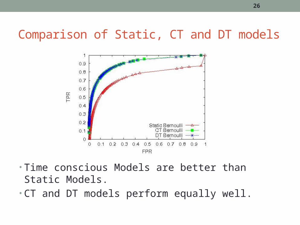
Comparison of Static, CT and DT models

• Time conscious Models are better than Static Models.• CT and DT models perform equally well.

26

Runtime

• Static and DT models are far more efficient compared to CT models because of their incremental nature.

27

Testing

Predicting Time – Distribution of Error

• Operating Point is chosen corresponding to • TPR: 82.5%, FPR: 17.5%.

28

X-axis: error in predicting time (in weeks)

Y-axis: frequency of that error

Most of the time, error in the prediction is very small

Predicting Time – Coverage vs Error

29

Operating Point is chosen corresponding to TPR: 82.5%, FPR: 17.5%.

A point (x,y) here means for y% of cases, the error is within

In particular, for 95% of the cases, the error is within 20 weeks.

x

User Influenceability

• Some users are more prone to influence propagation than others.

• Learn from Training data

30

Users with high influenceability => easier prediction of influence => more prone to viral marketing campaigns.

Action Influenceability

• Some actions are more prone to influence propagation than others.

31

Actions with high action influenceability => easier prediction of influence => more suitable to viral marketing campaigns.

Conclusions (1/2)• Previous works typically assume influence probabilities

are given as input.

• Studied the problem of learning such probabilities from a log of past propagations.

• Proposed both static and time-conscious models of influence.

• Proposed efficient algorithms to learn and apply the models.

32

Conclusions (2/2)• Using CT models, it is possible to predict even the time at

which a user will perform it with a good accuracy.

• Introduce metrics of users and actions influenceability. • High values => easier prediction of influence.• Can be utilized in Viral Marketing decisions.

33

Q&A

Thanks!