learning object location predictors with boosting and … · eads, et al.: location-based,...

EADS, et al.: LOCATION-BASED, GRAMMAR-GUIDED OBJECT DETECTION 1

Learning Object Location Predictors withBoosting and Grammar-Guided FeatureExtraction

Damian Eads1

http://www.cs.ucsc.edu/~eads

Edward Rosten2

http://mi.eng.cam.ac.uk/~er258

David Helmbold1

http://www.cs.ucsc.edu/~dph

1 Department of Computer ScienceUniversity of CaliforniaSanta Cruz, California, USA

2 Department of EngineeringUniversity of CambridgeCambridge, UK

Abstract

We present BEAMER: a new spatially exploitative approach to learning object de-tectors which shows excellent results when applied to the task of detecting objects ingreyscale aerial imagery in the presence of ambiguous and noisy data. There are fourmain contributions used to produce these results. First, we introduce a grammar-guidedfeature extraction system, enabling the exploration of a richer feature space while con-straining the features to a useful subset. This is specified with a rule-based generativegrammar crafted by a human expert. Second, we learn a classifier on this data usinga newly proposed variant of AdaBoost which takes into account the spatially correlatednature of the data. Third, we perform another round of training to optimize the method ofconverting the pixel classifications generated by boosting into a high quality set of (x,y)locations. Lastly, we carefully define three common problems in object detection and de-fine two evaluation criteria that are tightly matched to these problems. Major strengths ofthis approach are: (1) a way of randomly searching a broad feature space, (2) its perfor-mance when evaluated on well-matched evaluation criteria, and (3) its use of the locationprediction domain to learn object detectors as well as to generate detections that performwell on several tasks: object counting, tracking, and target detection. We demonstratethe efficacy of BEAMER with a comprehensive experimental evaluation on a challengingdata set.

1 IntroductionLearning to detect objects is a subfield of computer vision that is broad and useful withmany applications. This paper is concerned with the task of unstructured object detection:the input to the object detector is an image with an unknown number of objects present,and the output is the locations of the objects found in the form of (x,y) pairs, and perhapsdelineating them as well. A typical application is detection of cars in aerial imagery forpurposes such as car counting for traffic analysis, tracking, or target detection. Figure 1shows (a) an example image from the data set used in the experiments, (b) its mark-up, (c)

c© 2009. The copyright of this document resides with its authors.It may be distributed unchanged freely in print or electronic forms.

BMVC 2009 doi:10.5244/C.23.92

2 EADS, et al.: LOCATION-BASED, GRAMMAR-GUIDED OBJECT DETECTION

(d) (e) (f)

(a) (b) (c) (g) (h) (i)

Figure 1: An aerial photo of Phoenix, AZ was divided into 11 slices. An example slice isshown in subfigure (a). Its mark-up is shown in subfigure (b); background pixels are black,object pixels are grey, and confuser pixels, white. Subfigure (c) shows an example of a postprocessing applied to a weak hypothesis, which helps disambiguate between similar car andbuilding patches by abstaining on building pixels. Cars are indicated by red, background byblue and abstention by green. Examples of ambiguous objects include (d) a roof-mountedair-conditioner, (e) an overhead street sign, (f) vegetation, (g) closely packed cars, (h) a darkcar, and (i) a car on a roof carpark in partial shadow.

an example of an initial confidence-rated weak hypothesis learned on it, and subfigures (d-i)show some of the trickier examples in the data set.

Section 2 reviews common approaches to object detection. Section 3.2 describes a newvariant of AdaBoost that takes into account the spatially correlated nature of the data to re-duce the effects of label noise, simplify solutions, and achieve good accuracy with fewerfeatures. Section 3.1 describes our technique for generating features randomly but guidedby a stochastic grammar crafted by a domain expert to make useful features more likely, andunhelpful features, less likely. A second round of training involves learning detectors whichpredict (x,y) locations of objects from pixel classifications, described in Section 3.3. Sincethe quality of detections greatly depends on the problem at hand, two different evaluationcriteria are carefully formulated to closely match three common problems: tracking, targetdetection, and object counting. Lastly, in our evaluation Section 4, each component in thedetection pipeline is isolated and compared against alternatives through an extensive vali-dation step involving a grid search over many parameters on the two different metrics. Theresults are used to gain insights into what leads to a good object detector. We have found ourcontributions give better results.

2 Background

Localizing objects in an image is a prevalent problem in computer vision known as objectdetection. Object recognition, on the other hand, aims to identify the presence or absence ofan object in an image. Many object detection approaches reduce object detection to objectrecognition by employing a sliding window [8, 12, 22], one of the more common designpatterns of an object detector. A fixed sized rectangular or circular window is slid acrossan image, and a classifier is applied to each window. The classifier usually generates areal-valued output representing confidence of detection. Often this method must carefully


arbitrate between nearby detections to achieve adequate performance.Object detection models can be loosely be broken down into several different overlap-

ping categories. Parts-based based models consider the presence of parts and (usually) thepositioning of parts in relation to one another [1, 3, 7]. A special case is the bag of wordsmodel where predictions are made simply on the presence or absence of parts rather thantheir overall structure or relative positions [10, 23]. Some parts-based models model objectsby their characterizing shape during learning and matching shape to detect [2]. Cascadesare commonly used to reduce false positives and improve computational efficiency. Ratherthan applying a single computationally expensive classifier to each window, a sequence ofcheaper classifiers is used. Later classifiers are invoked only if the previous classifiers gen-erate detections. Generative model approaches learn a distribution on object appearances orobject configurations [14]. Segmentation-based approaches fully delineate objects of interestwith polygons or pixel classification [20]. Contour-based approaches identify contours in animage before generating detections [8, 15]. Descriptor vector approaches generate a set offeatures on local image patches. One of the most commonly used descriptors is the Scale In-variant Feature Transform (SIFT), which is invariant to rotation, scaling, and translation androbust to illumination and affine transformations [13]. A large number of object detectorsuse interest point detectors to find salient, repeatable, and discriminative points in the imageas a first step [1, 5]. Feature descriptor vectors are often computed from these interest points.Probabilistic models estimate the probability of an object of interest occurring; generativemodels are often used [7, 19]. Feature Extraction creates higher level representations of theimage that are often easier for algorithms to learn from. Heisele, et al. [10] train a two-levelhierarchy of support vector machines: the first level of SVMs finds the presence of parts,and these outputs are fed into a master SVM to determine the presence of an object. Dorko,et al. [5] use an interest point detector, generate a SIFT description vector on the interestpoints, and then use an SVM to predict the presence or absence of objects.

One of the more popular and highly regarded feature-based object detectors is the slid-ing window detector proposed by Viola and Jones [22], which uses a feature set originallyproposed by Papageorgiou, et al. [16]. Adjacent rectangles of equal size are filled with 1sand −1s and embedded in a kernel filled with zeros. The kernel is convolved with the imageto produce the feature and using an integral image greatly reduces the computation time forthese features. Viola and Jones employ a cascaded sliding window approach where eachcomponent classifier of the cascade is a linear combination of weak classifiers trained withAdaBoost.

3 ApproachThe BEAMER object detector pipeline consists of a feature extraction stage, pixel classifica-tion stage, and a detector stage as Figure 2 shows. First, a set of learned features are com-bined into a pixel classifier using AdaBoost [9]. Then, the detector pipeline (see Section 3.3)transforms the pixel classifications into a set of (x,y) locations representing the predictedlocations of the objects. Our methodology partitions the data set into training, validation,and test image sets. The pixel classifier is learned during the training phase on the trainingimages with the grammar constraints, post-processing parameters, and stopping conditionsremaining fixed. These fixed parameters are later tuned on the validation set along with thedetector’s parameters. The detector generates (x,y) location predictions from the pixel clas-sification. After the training and validation steps, a fully learned object detector results. The


FeatureExtractor

FeatureExtractor

FeatureExtractor

FeatureExtractorFeatureExtractorFeatureExtractor

>= a

< b

>= c

Region Grow [t=500]

Erode [r=2],Dilate [r=3]

Region Grow [t=1000]

WeightedSum

GrammarFeature(X)->...

Detector

(x,y)

(x,y)

(x,y)

ScoringMetric

Hit

Miss

Hit

ROC Curve

Feature Extraction Apply Decision Stumps Postprocessing

Boosting Ensemble

Features Weak Hypotheses

Confidence Image

Selected with AdaBoostScores Final Detections

Parameters Selected through Validation

Figure 2: Object detection is carried out in a pipeline consisting of three stages: featureextraction, pixel classification, and locality predictions in the form of (x,y). At each trainingiteration, a new pool of feature extractors generated by a grammar. BEAMER then choosesthe best feature extractor, decision stump, and post-processing filter combination. Thresh-olding these features yields a weak pixel classification which are combined with AdaBoostto produce a confidence image. The grey arrows show the flow of data to carry out objectdetection from start to finish for a static instance of an object detector.

grey arrows show how data flows through a specific instance of an object detector.Section 3.1 describes the very first step of weak pixel classification, feature extraction,

which is carried out by generating features with a generative grammar. Section 3.2 describesthe learning of an ensemble of weak pixel classifications using boosting. Finally, Section 3.3explains how the pixel classification ensemble is transformed into (x,y) location domainpredictions. A complete list of all the parameters described in the following sections is givenin Table 2.

3.1 Feature ExtractionA single pixel in a greyscale image provides very limited information about its class. Featureextraction is helpful for generating a more informative feature vector for each pixel, ideallyincorporating spatial, shape, and textural information. This paper considers extracting fea-tures with neighborhood image operators such as convolution and morphology. Even goodsets of neighborhood-based features are unlikely to have enough information to perfectlypredict labels, but the hope is that large and diverse sets of features can encode enough in-formation to make adequate predictions. At each boosting iteration, a new set of randomfeatures is generated, but only the best feature of this set is kept.

Generative grammars are common structures used in Computer Science to specify rulesto define a set of strings [11, 21]. Extending our earlier work on time series [6], we use themto specify the space of feature extraction programs, which are represented as directed graphs(a graph representation is preferable because it allows for re-use of sub-computations). Agrammar is made up of nonterminal productions such as P → A|B, which are expanded togenerate a new string. The rules associated with the production are selected at random, soP can be expanded as either A or B. Figure 3 shows an example graph program generated


I

‘ellipse’, π

2 ,8, .3

normDifferode

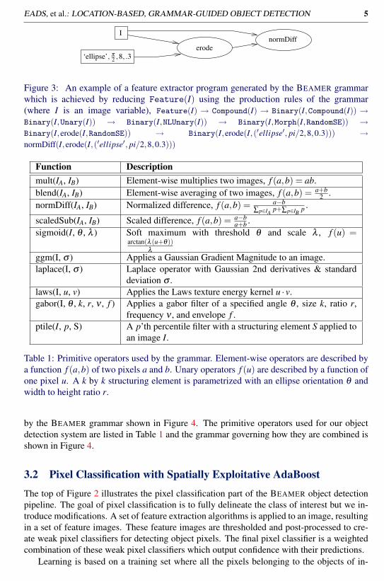
Figure 3: An example of a feature extractor program generated by the BEAMER grammarwhich is achieved by reducing Feature(I) using the production rules of the grammar(where I is an image variable), Feature(I) → Compound(I) → Binary(I,Compound(I)) →Binary(I,Unary(I)) → Binary(I,NLUnary(I)) → Binary(I,Morph(I,RandomSE)) →Binary(I,erode(I,RandomSE)) → Binary(I,erode(I,(′ellipse′, pi/2,8,0.3))) →normDiff(I,erode(I,(′ellipse′, pi/2,8,0.3)))

Function Descriptionmult(IA, IB) Element-wise multiplies two images, f (a,b) = ab.blend(IA, IB) Element-wise averaging of two images, f (a,b) = a+b

2 .normDiff(IA, IB) Normalized difference, f (a,b) = a−b

∑p∈IAp+∑p∈IB p .

scaledSub(IA, IB) Scaled difference, f (a,b) = a−ba+b .

sigmoid(I, θ , λ ) Soft maximum with threshold θ and scale λ , f (u) =arctan(λ (u+θ))

λ

ggm(I, σ ) Applies a Gaussian Gradient Magnitude to an image.laplace(I, σ ) Laplace operator with Gaussian 2nd derivatives & standard

deviation σ .laws(I, u, v) Applies the Laws texture energy kernel u · v.gabor(I, θ , k, r, ν , f ) Applies a gabor filter of a specified angle θ , size k, ratio r,

frequency ν , and envelope f .ptile(I, p, S) A p’th percentile filter with a structuring element S applied to

an image I.

Table 1: Primitive operators used by the grammar. Element-wise operators are described bya function f (a,b) of two pixels a and b. Unary operators f (u) are described by a function ofone pixel u. A k by k structuring element is parametrized with an ellipse orientation θ andwidth to height ratio r.

by the BEAMER grammar shown in Figure 4. The primitive operators used for our objectdetection system are listed in Table 1 and the grammar governing how they are combined isshown in Figure 4.

3.2 Pixel Classification with Spatially Exploitative AdaBoost

The top of Figure 2 illustrates the pixel classification part of the BEAMER object detectionpipeline. The goal of pixel classification is to fully delineate the class of interest but we in-troduce modifications. A set of feature extraction algorithms is applied to an image, resultingin a set of feature images. These feature images are thresholded and post-processed to cre-ate weak pixel classifiers for detecting object pixels. The final pixel classifier is a weightedcombination of these weak pixel classifiers which output confidence with their predictions.

Learning is based on a training set where all the pixels belonging to the objects of in-


Feature(X) → Binary(Unary(X),Unary(X))| NLUnary(Unary(X))| NLBinary(Unary(X),Unary(X))| Compound(X)

Binary(X ,Y ) → mult(X ,Y ) | normDiff(X ,Y ) | scaledSub(X ,Y ) | blend(X ,Y )NLBinary(X ,Y ) → mult(X ,Y ) | normDiff(X ,Y )

Unary(X) → LUnary(X) | NLUnary(X)Compound(X) → Unary(X) | Binary(X ,Compound(X))Morph(X ,S) → erode(X ,S) | dilate(X ,S) | open(X ,S) | close(X ,S)RandomSE() → (θ ∈ [0,2π],{2k +1|k ∈ {1, . . . ,7}},{102s−1|s ∈ [0,1]})NLUnary(X) → sigmoid(X ,a ∈ SNorm(),b ∈ {0.1,0})

| Morph(X ,RandomSE())| ptile(X , p ∈ [0,100],RandomSE())| ggm(X ,3∗SNorm())

LUnary(X) → laws(X ,u ∈ {L5,E5,S5,R5,W5},v ∈ {L5,E5,S5,R5,W5})| laplace(X ,σ ∈ 3∗SNorm())| gabor(X ,θ ∈ [0,π],k ∈ [1,31],{102q−1|q ∈ [0,1]},{10s+2|s ∈ [0,1]},sin|cos|both)| convolve(X ,ViolaJonesKernel())

Figure 4: The grammar used to generate features for the pixel classification stage of theobject detection system. The ViolaJonesKernel() does not sample uniformly from thespace of all kernels. Rather, the kernel type (horizontal-2, vertical-2, horizontal-3, vertical-3, quad) is chosen uniformly at random, followed by the size, then location. RandomSEdefines an elliptical structuring element, where the parameters of the ellipse are respectivelyorientation, major radius in pixels and aspect ratio. The meanings of the other parametersare given in Table 1.

(a) (b) (c) (d) (e)

Figure 5: Subfigures (b)-(e) are five examples of features generated by a grammar and ap-plied to the image shown in subfigure (a).

terest (cars in our case) are hand-labeled. There are several difficulties in identifying goodweak pixel classifiers from the hand-labeled training data. First, in applications like oursthere are many more background pixels than foreground (object) pixels. Providing too muchbackground puts too much emphasis on the background during learning, and can lead to hy-potheses that do not perform well on the foreground. Second, hand-labeling is a subjectiveand error prone activity. Pixels outside the border of the object may be accidentally labeledas car, and pixels inside the border as background. It is well known that label noise causes


difficulties for AdaBoost [4, 17]. This difficulty is compounded when the image data itself isnoisy or there may not be sufficient information in a pixel neighborhood to correctly classifyevery pixel. Third, training a pixel classifier that fully segments is a much harder problemthan localization. For example, if a weak hypothesis correctly labels only a tenth of theobject pixels and these correct predictions are evenly distributed throughout the objects, theweak hypothesis will appear unfavorable. This is unfortunate because the weak hypothesismay be very good at localizing objects, just not fully segmenting them. Similarly, some oth-erwise good features may identify many objects as well as large swaths of background. Interms of localization, the performance is good but these hypotheses will be rejected by thelearning algorithm because of the large number of false positives they produce.

We propose three spatially-motivated modifications to standard AdaBoost to performwell with the difficulties above. First, we weight the initial distribution so the sum of theforeground weight is proportionate with the background class. Second, we use confidence-rated AdaBoost proposed by Schapire and Singer [18] so weak hypotheses can output lowor zero confidence on pixels which may be noisy or labeled incorrectly. In confidence-rated boosting, the weak hypotheses output predictions from the real interval [−1,1] andthe more confident predictions are farther from zero. In the boosting literature, the edge isdefined as the weighted training error. Third, we perform post-processing on the weak pixelclassifications to improve those that produce good partial segmentations of objects.

Weak Classifier Post-processing Four different weak pixel classification post-processingfilters are considered and compared against no filtering at all. The first technique performsregion growing (abbreviated R) with a 4-connected flood fill. Regions larger than k pixelsare identified and converted to abstentions (zero confidence predictions). This is useful fordisambiguating cars from large swaths, such as buildings, which may have similar textureas cars. This simple post-processing filter works very well in practice. The other three post-processing techniques apply either an erosion (E), a dilation (D), or a local median filter(M) using a circular structuring element of radius r. When applying one of these filters, apixel classifier only partially labeling an object will be evaluated more favorably. This im-proves the stability of learning in situations where the object pixels are noisy in the imagesand pixels are mislabeled. Section 4 thoroughly compares the performance of different com-binations of these four post-processing filters, all of which show better performance than nofiltering at all.

3.3 Learning and Predicting in the (x,y) Location Domain

The final stage of object detection turns the confidence-rated pixel classification into a listof locations pointing to the objects in an image. Noisy and ambiguous data often reducethe quality of the pixel classification, but since we use pixel classification as a step alongthe way, we perform an extra round of training to learn to transform a rough labeling ofobject pixels into a high quality list of locality predictions, and to do so in a noise-robust andspatially exploitative manner. Pure pixel-based approaches are hard to optimize for location-based criteria, and often translate mislabeled pixels into false positives. Our algorithms turnthe pixel classifications into a list of object locations, allowing us to operate in and directlyoptimize over the same domain as the output: a list of (x,y) locations.

A confidence-rated pixel classification provides predictive power about which pixels arelikely to belong to an object. The goal is a high quality localization, rather than object


delineation, so we reduce the set of positive pixels to a smaller set of high-quality locations.The first object detector, Connected Components (CC) thresholds the confidence imageat zero, performs binary dilation with a circular structuring element of radius σCC, findsconnected components and marks detections at the centroids of the components.

Large Local Maxima (LLM), is like non-maximal suppression but instead representsthe locations and magnitudes of the maxima in location space as opposed to image space.The approach sparsifies the set of high confidence pixels by including only local maximaas guesses of an object’s location. Next, the LLM detector chooses among the set of localmaxima those pixel locations with confidences exceeding a threshold θLLM . This method ofdetection is attractive because it is very fast, and somewhat reminiscent of decision stumps.The detector outputs these large maxima as its final predictions, ordering them with decreas-ing confidence. A Gaussian smoothing of width σLLM can be applied before finding themaxima to reduce the noise and further refine the solutions.

The LLM detector treats maxima locations independently, which can be quite sensitiveto the presence of outlier pixels and noisy imagery. Noisy imagery often leads to an excessof local maxima, some of which lie outside an object’s boundary, which often results infalse positives. We propose an extension of the LLM detector called the Kernel DensityEstimate (KDE) detector for combining maxima locations into a smaller, higher qualityset of locations based on large numbers of maxima with high confidence clustered spatiallyclose to one another. More specifically, the final detections are the modes of a confidence-weighted Kernel Density Estimate computed over the set of LLM locations. The width of thekernel is denoted σKDE . Our results show the KDE and LLM detectors perform remarkablywell in the presence of noise.

4 Evaluation and Conclusions

Generating a ROC curve for a classifier involves marking each classification as a true nega-tive or false positive. Quantifying the accuracy of unstructured object detection with a ROCcurve is not as straightforward: the criteria for marking a true positive or false positive de-pends on the object detection task at hand. We consider three object detection problems:cueing, tracking, and counting and define two criteria to mark detections that are closelymatched with these problems. Points on the ROC curves are then drawn using predictedlocations above some confidence threshold.

The goal of the cueing task is to output detections within the delineation of the object.False positives away from objects are penalized, but multiple true positives are not. Figure 6,subfigures (a-c) show the results for this metric.

We introduce the nearest neighbors criteria for marking detections for object tracking.Good detectors for tracking localize objects within some small error, and multiple detectionsof a given object are penalized. At each threshold the criteria finds the detection closest toan object. This pair is removed and the process is repeated until either no detections or noobjects remain, or the distance of all remaining pairs exceeds a radius, r. Remaining objectsare false negatives and remaining detections are false positives.

Lastly the task of object counting is concerned less with localization and more withaccurate counts. We employ the nearest neighbors criteria for this purpose but to loosen thedesire for a spatial correlation between detections and object locations, we set the nearestneighbor radius threshold r to a high value.


0.0 0.2 0.4 0.6 0.8 1.0 1.2 1.4Mean FP Per Image/Mean # of Objects Per Image

0.0

0.2

0.4

0.6

0.8

1.0D

ete

ctio

n R

ate

Grammars and Postprocessing [Cueing]

Grammar w/ PPGrammar w/o PPHaar w/ PPHaar w/o PPRandom


0.0

0.2

0.4

0.6

0.8

1.0

Dete

ctio

n R

ate

Comparison of Postprocessors [Cueing]

No FilteringRE,DE,D,MR,E,D,MRandom


0.0

0.2

0.4

0.6

0.8

1.0

Dete

ctio

n R

ate

Comparison of Detectors [Cueing]

Best KDEBest LLMBest CCRandom

(a) (b) (c)


0.0

0.2

0.4

0.6

0.8

1.0

Dete

ctio

n R

ate

Grammars and Postprocessing [NN Metric r=10]

Grammar w/ PPGrammar w/o PPHaar w/ PPHaar w/o PPRandom


0.0

0.2

0.4

0.6

0.8

1.0

Dete

ctio

n R

ate

Comparison of Postprocessors [NN Metric r=10]

No FilteringRE,DE,D,MR,E,D,MRandom


0.0

0.2

0.4

0.6

0.8

1.0

Dete

ctio

n R

ate

Comparison of Detectors [NN Metric r=10]

Best KDEBest LLMBest CCRandom

(d) (e) (f)

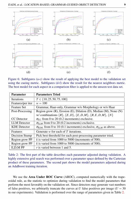
Figure 6: Subfigures (a-c) show the result of applying the best model to the validation setusing the cueing metric. Subfigures (d-f) show the result for the nearest neighbors metric.The best model for each aspect in a comparison filter is applied to the unseen test data set.

Parameter Parameters TriedIterations T ∈ {10,25,50,75,100}Features/per iter w = 100Feature Set Grammar, Haar-only, Grammar w/o Morphology or w/o HaarPost-Processing Region grow (R), Erosion (E), Dilation (D), Median (M), None (N)

w/ combinations {R}, {E,D}, {E,D,M}, {R,E,D,M}, {N}CC Detector σCC from 0 to 20 (0.2 increments) exclusive.LLM Detector σLLM from 0 to 20 (0.2 increments) exclusive.KDE Detector σKDE from 0 to 10 (0.1 increments) exclusive, σLLM as above.Features Generate w for each of T iterations.Decision Stump Pick best threshold for each post-processing parameter tried.Region grow PP k is varied from 1000 to 5000 (increments of 500).Region grow PP k is varied from 1000 to 5000 (increments of 500).E,D,M PP r is varied between 1 and 5.

Table 2: The first part of the table describes each parameter adjusted during validation. Ahighly extensive grid search was performed over a parameter space defined by the Cartesianproduct of these parameters. The second part shows the model parameters adjusted duringan AdaBoost training iteration.

We use the Area Under ROC Curve (AROC), computed numerically with the trape-zoidal rule, as the statistic to optimize during validation to find the model parameters thatperform the most favorably on the validation set. Since detectors may generate vast numbersof false positives, we arbitrarily truncate the curves at U false positives per image (U = 30in our experiments). Validation is performed over the range of parameters given in Table 2.


Figure 6 illustrates the results of applying the most favorable models and parameter vec-tors (determined using the validation data) to the test set. Subfigure (a)–(c) and (d)–(f) illus-trate the performance using the cueing and tracking metrics. Subfigures (a) and (d) show theclear advantage of using post-processing and grammar-guided features over just Haar-likefeatures. Subfigure (b) and (e) show the benefit of post-processing for reducing the effects oflabel and image noise, and clearly highlights the need to properly tune parameters throughvalidation and train all stages for each problem. Region growing performs better on the near-est neighbors metric–unsurprising as it abstains on ambiguous background patches, reducingfalse positives. On the cueing metric, morphology helps in reducing the effects of label noise,which often leads to false positives outside an object delineation. Finally subfigures (c) and(f) show that the spatially exploitative detection algorithms LLM and KDE outperform thepixel-based CC detector.

References[1] Shivani Agarwal, Aatif Awan, and Dan Roth. Learning to Detect Objects in Images

via a Sparse, Part-Based Representation. IEEE Transactions on Pattern Analysis andMachine Intelligence, pages 1475–1490, 2004.

[2] Serge Belongie, Jitendra Malik, and Jan Puzicha. Shape matching and object recogni-tion using shape contexts. IEEE Transactions on Pattern Analysis and Machine Intel-ligence, 24:509–522, 2002.

[3] Ondrej Chum and Andrew Zisserman. An exemplar model for learning object classes.IEEE Conference on Computer Vision and Pattern Recognition, pages 1–8, 2007.

[4] Thomas G. Dietterich. An Experimental Comparison of Three Methods for Construct-ing Ensembles of Decision Trees: Bagging Boosting, and Randomization. MachineLearning, 40(2):139–157, 2000.

[5] Gyuri Dorkó and Cordelia Schmid. Selection of scale-invariant parts for object classrecognition. IEEE International Conference on Computer Vision, 1:634, 2003.

[6] Damian Eads, Karen Glocer, Simon Perkins, and James Theiler. Grammar-guidedfeature extraction for time series classification. Technical Report LA-UR-05-4487,Los Alamos National Laboratory, MS D436, Los Alamos, NM, 87545, June 2005.

[7] Rob Fergus, Pietro Perona, and Andrew Zisserman. Object class recognition by unsu-pervised scale-invariant learning. IEEE Conference on Computer Vision and PatternRecognition, 2:264, 2003.

[8] Vittorio Ferrari, Loic Fevrier, Frédéric Jurie, and Cordelia Schmid. Groups of adjacentcontour segments for object detection. IEEE Transactions on Pattern Analysis andMachine Intelligence, 30(1):36–51, January 2008.

[9] Yoav Freund and Robert E. Schapire. Experiments with a new boosting algorithm. InInternational Conference on Machine Learning, pages 148–156, 1996.

[10] Bernd Heisele, Purdy Ho, Jane Wu, and Tomaso Poggio. Face recognition: component-based versus global approaches. Computer Vision and Image Understanding, 91(1-2):6–21, 2003.


[11] John Hopcroft and Jeffrey Ullman. Introduction To Automata Theory, Languages, AndComputation. Addison-Wesley, 1990.

[12] Ivan Laptev. Improvements of object detection using boosted histograms. British Ma-chine Vision Conference, 3:949–958, 2006.

[13] David G. Lowe. Object recognition from local scale-invariant features. IEEE Interna-tional Conference on Computer Vision, 2:1150, 1999.

[14] Kristian Mikolajczyk, Bastian Leibe, and Bernt Schiele. Multiple Object Class Detec-tion with a Generative Model. Computer Vision and Pattern Recognition, pages 26–36,2006.

[15] Andreas Opelt, Axel Pinz, and Andrew Zisserman. A Boundary-Fragment-Model forObject Detection. Lecture Notes in Computer Science, 3952:575, 2006.

[16] Constantine P. Papageorgiou, Michael Oren, and Tomaso Poggio. A general frameworkfor object detection. IEEE International Conference on Computer Vision, pages 555–562, 1998.

[17] Gunnar Rätsch, Takashi Onoda, and Klaus Müller. Soft margins for AdaBoost. Ma-chine Learning, 42(3):287–320, 2001.

[18] Robert Schapire and Yoram Singer. Improved boosting algorithms using confidence-rated predictions. Machine Learning, 37(3):297–336, 1999.

[19] Henry Schneiderman and Takeo Kanade. A statistical method for 3d object detectionapplied to faces and cars. IEEE Conference on Computer Vision and Pattern Recogni-tion, page 1746, 2000.

[20] Jamie Shotton, Matthew Johnson, and Roberto Cipolla. Semantic Texton Forests forImage Categorization and Segmentation. In IEEE Conference on Computer Vision andPattern Recognition, pages 1–8, 2008.

[21] Michael Sipser. Introduction to the Theory of Computation. International ThomsonPublishing, 2005.

[22] Paul Viola and Michael Jones. Rapid object detection using a boosted cascade of simplefeatures. Computer Vision and Pattern Recognition, IEEE Computer Society Confer-ence on, 1:511, 2001.

[23] Jianguo Zhang, Marcin Marszalek, Svetlana Lazebnik, and Cordelia Schmid. Localfeatures and kernels for classification of texture and object categories: A comprehen-sive study. International Journal of Computer Vision, 73(2):213–238, 2007.

learning object location predictors with boosting and … · eads, et al.: location-based,...

Documents