learning parameters in discrete naive bayes models by computing
TRANSCRIPT
Learning Parameters in Discrete Naive
Bayes models by Computing Fibers of the
Parametrization Map
Vincent Auvray and Louis Wehenkel
EE & CS Dept. and GIGA-R, University of Liège, Belgium
NIPS - AML 2008 - Whistler
1/26

Naive Bayesian networks
A discrete naive Bayesian network (or latent class model) with
m classes is a distribution p over discrete variables X1, . . . , Xn
such that
p(X1 = x1, . . . , Xn = xn) =
m∑
t=1
p(C = t)
n∏
i=1
p(Xi = xi |C = t).
Graphically, the independencies between C, X1, . . . , Xn are
encoded by
C
}}||||
|
!!CC
CCC
X1 · · · Xn
2/26
Problem statement
Given a naive Bayesian network p, compute the parameters
p(C = t), p(Xi = xi |C = t) for i = 1, . . . , n, t = 1, . . . , m, and
xi ∈ Xi mapped to p.
Why?
• better understanding of the model
• estimation of parameters
• model selection
• study of parameter identifiability
3/26

Outline
Mathematical Results
Applications
Extension
4/26

Some notation
Given parameters of a naive Bayesian distribution, we define
new parameters
wt = p(C = t),
Atxi
= p(Xi = xi |C = t) − p(Xi = xi).
Given a distribution p, let
q(xi1 , . . . , xik ) = p(xi1 , . . . , xik )
−∑
{Xj1,...,Xjl
}({Xi1,...,Xik
}
q(xj1 , . . . , xjl )
∏
Xk∈{Xi1,...,Xik
}\{Xj1,...,Xjl
}
p(xk ).
5/26
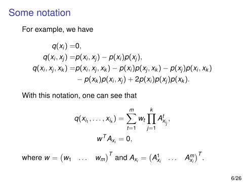
Some notation
For example, we have
q(xi ) =0,
q(xi , xj ) =p(xi , xj) − p(xi)p(xj),
q(xi , xj , xk ) =p(xi , xj , xk ) − p(xi)p(xj , xk ) − p(xj)p(xi , xk )
− p(xk )p(xi , xj) + 2p(xi)p(xj)p(xk ).
With this notation, one can see that
q(xi1 , . . . , xik ) =m∑
t=1
wt
k∏
j=1
Atxij
,
wT Axi= 0,
where w =(
w1 . . . wm
)Tand Axi
=(
A1xi
. . . Amxi
)T.
6/26
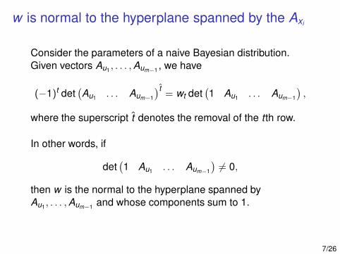
w is normal to the hyperplane spanned by the Axi
Consider the parameters of a naive Bayesian distribution.
Given vectors Au1, . . . , Aum−1
, we have
(−1)t det(
Au1. . . Aum−1
)t= wt det
(
1 Au1. . . Aum−1
)
,
where the superscript t denotes the removal of the t th row.
In other words, if
det(
1 Au1. . . Aum−1
)
6= 0,
then w is the normal to the hyperplane spanned by
Au1, . . . , Aum−1
and whose components sum to 1.
7/26

The components of Axiare the roots
of a degree m polynomial
For m = 2, we have
s2q(u1, v1) + sq(xi , u1, v1) − q(xi , u1)q(xi , v1)
= q(u1, v1)(s + A1xi)(s + A2
xi).
For m = 3, we have
s3 det(
q(u1,v1) q(u1,v2)q(u2,v1) q(u2,v2)
)
+ s2[
det(
q(u1,v1) q(u1,v2)q(xi ,u2,v1) q(xi ,u2,v2)
)
+ det(
q(xi ,u1,v1) q(xi ,u1,v2)q(u2,v1) q(u2,v2)
)]
+s[
− det(
q(u1,v1) q(u1,v2)q(xi ,u2)q(xi ,v1) q(xi ,u2)q(xi ,v2)
)
− det(
q(xi ,u1)q(xi ,v1) q(xi ,u1)q(xi ,v2)q(u2,v1) q(u2,v2)
)
+ det(
q(xi ,u1,v1) q(xi ,u1,v2)q(xi ,u2,v1) q(xi ,u2,v2)
)]
−det(
q(xi ,u1,v1) q(xi ,u1,v2)q(xi ,u2)q(xi ,v1) q(xi ,u2)q(xi ,v2)
)
−det(
q(xi ,u1)q(xi ,v1) q(xi ,u1)q(xi ,v2)q(xi ,u2,v1) q(xi ,u2,v2)
)
= det(
q(u1,v1) q(u1,v2)q(u2,v1) q(u2,v2)
)
(s + A1xi)(s + A2
xi)(s + A3
xi).
8/26

The components of Axiare the roots
of a degree m polynomial
Given u = {u1, . . . , um−1} and v = {v1, . . . , vm−1}, consider
the polynomial of degree m
αx,u,v(s) = sm det
(
q(u1,v1) ··· q(u1,vm−1)
......
q(um−1,v1) ··· q(um−1,vm−1)
)
+ sm−1 · · · + s · · · + . . .
whose coefficients are sums of determinants. We have
αx,u,v(s) = det
(
q(u1,v1) ··· q(u1,vm−1)
......
q(um−1,v1) ··· q(um−1,vm−1)
)
m∏
t=1
(s + Atxi).
9/26

The parameters satisfy simple polynomial equations
Consider values {x1, . . . xk}. The following equation holds
det
∏kj=1 At
xjq(x1, . . . , xk , v1) . . . q(x1, . . . , xk , vm−1)
Atu1
q(u1, v1) . . . q(u1, vm−1)...
......
Atum−1
q(um−1, v1) . . . q(um−1, vm−1)
= q(x1, . . . , xk ) det
q(u1, v1) · · · q(u1, vm−1)...
...
q(um−1, v1) · · · q(um−1, vm−1)
.
10/26

The parameters satisfy simple polynomial equations
For {x1, . . . xk} = {u0}, we have
det
Atu0
q(u0, v1) . . . q(u0, vm−1)
Atu1
q(u1, v1) . . . q(u1, vm−1)...
......
Atum−1
q(um−1, v1) . . . q(um−1, vm−1)
= 0.
For m = 3 and {x1, . . . xk} = {u1, u2}, we have
det
Atu1
Atu2
q(u1, u2, v1) q(u1, u2, v2)
Atu1
q(u1, v1) q(u1, v2)
Atu2
q(u2, v1) q(u2, v2)
= q(u1, u2) det
(
q(u1, v1) q(u1, v2)q(u2, v1) q(u2, v2)
)
.
11/26

Some determinants have an interpretable
decomposition
Consider sets of values s1, . . . sm−1. We have
det
q(s1, v1) . . . q(s1, vm−1)...
...
q(sm−1, v1) . . . q(sm−1, vm−1)
=(
m∏
t=1
wt
)
det(
1 Av1. . . Avm−1
)
det M,
where
M =
1∏
x∈s1A1
x . . .∏
x∈sm−1A1
x
......
...
1∏
x∈s1Am
x . . .∏
x∈sm−1Am
x
12/26

Simple implicit equations follow
Consider a naive Bayesian distribution with m classes and
consider sets of values s1, . . . , sm′−1. If m′ > m, we have
det
q(s1,v1) ... q(s1,vm′−1)
......
q(sm′−1,v1) ... q(sm′
−1,vm′−1)
= 0.
Consider sets of values s1, . . . , sm−1 and r1, . . . , rm−1. We
have
det
(
q(s1,v1) ... q(s1,vm−1)
......
q(sm−1,v1) ... q(sm−1,vm−1)
)
det
(
q(r1,u1) ... q(r1,um−1)
......
q(rm−1,u1) ... q(rm−1,um−1)
)
= det
(
q(s1,u1) ... q(s1,um−1)
......
q(sm−1,u1) ... q(sm−1,um−1)
)
det
(
q(r1,v1) ... q(r1,vm−1)
......
q(rm−1,v1) ... q(rm−1,vm−1)
)
13/26

Outline
Mathematical Results
Applications
Extension
14/26
Potential applications of our results
• Compute the set of parameters mapped to a given naive
Bayesian distribution
• Estimate parameters from data by applying the previous
computation to the distribution of observed frequencies
• Derive sufficient conditions for parameter identifiability
and obtain results on the dimensionality of the model
• Building block in the computation of analytic asymptotic
approximations to the marginal likelihood of the model
• Building block in model selection and learning of hidden
causes
15/26

An important hypothesis to compute the parameters
Suppose that we have a distribution p and sets of values
t = {t1, . . . , tm−1},
u = {u1, . . . , um−1},
v = {v1, . . . , vm−1}
such that
det
(
q(t1,u1) ... q(t1,um−1)
......
q(tm−1,u1) ... q(tm−1 ,um−1)
)
6= 0,
det
(
q(t1,v1) ... q(t1,vm−1)
......
q(tm−1,v1) ... q(tm−1 ,vm−1)
)
6= 0,
det
(
q(u1,v1) ... q(u1,vm−1)
......
q(um−1,v1) ... q(um−1,vm−1)
)
6= 0.
16/26

Computation of w from Au1, . . . , Aum−1
Our hypothesis amounts to
(
m∏
i=1
wi
)
det(
1 At1 . . . Atm−1
)
det(
1 Au1. . . Aum−1
)
det(
1 Av1. . . Avm−1
)
6= 0.
Hence, we have
wi =(−1)i det
(
Au1. . . Aum−1
)i
det(
1 Au1. . . Aum−1
) .
17/26

Computation of Ax from Au1, . . . , Aum−1
Since
det
Atu1
q(u1,v1) ... q(u1,vm−1)
......
...At
um−1q(um−1,v1) ... q(um−1,vm−1)
Atx q(x,v1) ... q(x,vm−1)
= 0,
we have, for all values x distinct of v1, . . . , vm−1,
ATx =
(
q(x , v1) . . . q(x , vm−1))
q(u1, v1) . . . q(u1, vm−1)...
...
q(um−1, v1) . . . q(um−1, vm−1)
−1
(
Au1. . . Aum−1
)T.
18/26

Computation of Au1, . . . , Aum−1
Find the roots of the polynomials νui ,t,vto obtain
{A1u1
, . . . , Amu1},
...
{A1um−1
, . . . , Amum−1
}.
Note that these sets are not ordered: we are not able to
assign each element to its hidden class.
There is some trivial non-identifiability due to the fact that
classes can be permuted freely. To remove this degree of
freedom from the analysis, we order the set {A1u1
, . . . , Amu1}
arbitrarily.
19/26
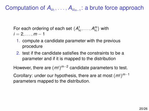
Computation of Au1, . . . , Aum−1
: a brute force approach
For each ordering of each set {A1ui
, . . . , Amui} with
i = 2, . . . , m − 1
1. compute a candidate parameter with the previous
procedure
2. test if the candidate satisfies the constraints to be a
parameter and if it is mapped to the distribution
However, there are (m!)m−2 candidate parameters to test.
Corollary: under our hypothesis, there are at most (m!)m−1
parameters mapped to the distribution.
20/26
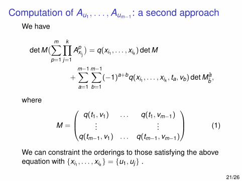
Computation of Au1, . . . , Aum−1
: a second approach
We have
det M(
m∑
p=1
k∏
j=1
Apxij
)
= q(xi1 , . . . , xik ) det M
+
m−1∑
a=1
m−1∑
b=1
(−1)a+bq(xi1 , . . . , xik , ta, vb) det M ab,
where
M =
q(t1, v1) . . . q(t1, vm−1)...
...
q(tm−1, v1) . . . q(tm−1, vm−1)
(1)
We can constraint the orderings to those satisfying the above
equation with {xi1 , . . . , xik } = {u1, uj} .
21/26

Computation of Au1, . . . , Aum−1
The previous algorithm do not make use of all our theoretical
results. For m = 3, recall that we have
det
Atu1
Atu2
q(u1, u2, v1) q(u1, u2, v2)
Atu1
q(u1, v1) q(u1, v2)
Atu2
q(u2, v1) q(u2, v2)
= q(u1, u2) det
(
q(u1, v1) q(u1, v2)q(u2, v1) q(u2, v2)
)
.
We can derive Atu2
from Atu1
by solving the above equation.
We are currently investigating how to make use of all our
results in the general case.
22/26

The inversion algorithms can be adapted to estimate
parameters
• Basic idea: apply the inversion algorithm to the observed
distribution p.
• Instead of testing whether a candidate parameter is
mapped to p, we find the parameter minimizing the
relative entropy to p.
• Suppose that the unknown p is a naive Bayesian
distribution with m classes satisfying our inversion
assumption. As the sample size increases, p converges
to p and, by continuity, our estimate converges to a true
parameter mapped to p.
23/26

Practical issues
The estimation procedure has several issues:
• The computational complexity grows extremely fast with
m, but linearly with n.
• The estimates are numerically unstable and require large
sample sizes. For smaller sample sizes, there may not
even be a single candidate parameter satisfying the
parameter constraints.
• There are many degrees of freedom in the choice of t, u
and v. Asymptotically, any choice is suitable. For small
sample size, it is probably important.
• The results are not competitive with the E.M. algorithm.
24/26

Extension to hierarchical latent class models
C1
vvnnnnnnnnnnn
��((PPPPPPPPPPP
C2
~~}}}}
}
�� BB
BBB
X4 C3
~~}}}}
}
�� BB
BBB
X1 X2 X3 X5 X6 X7
The parameters mapped to a HLC distribution with the above
structure can be derived from the parameters mapped to the
naive Bayesian distributions over
{X1, X2, X3}
{X1, X4, X5}
{X5, X6, X7}
obtained by marginalization.
25/26
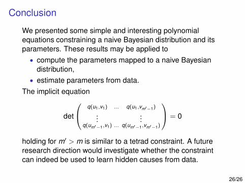
Conclusion
We presented some simple and interesting polynomial
equations constraining a naive Bayesian distribution and its
parameters. These results may be applied to
• compute the parameters mapped to a naive Bayesian
distribution,
• estimate parameters from data.
The implicit equation
det
q(u1,v1) ... q(u1,vm′−1)
......
q(um′−1,v1) ... q(um′
−1,vm′−1)
= 0
holding for m′ > m is similar to a tetrad constraint. A future
research direction would investigate whether the constraint
can indeed be used to learn hidden causes from data.
26/26