Learning Prosodic Sequences Usingthe Fundamental Frequency Variation Spectrum

Kornel Laskowski1, Jens Edlund2, and Mattias Heldner2

1 interACT, Carnegie Mellon University, Pittsburgh PA, USA2 Centre for Speech Technology, KTH, Stockholm, Sweden

kornel@cs.cmu.edu

Abstract

We investigate a recently introduced vector-valued representa-tion of fundamental frequency variation, whose properties ap-pear to be well-suited for statistical sequence modeling. Weshow what the representation looks like, and apply hiddenMarkov models to learn prosodic sequences characteristic ofhigher-level turn-taking phenomena. Our analysis shows thatthe models learn exactly those characteristics which have beenreported for the phenomena in the literature. Further refine-ments to the representation lead to a 12-17% relative improve-ment in speaker change prediction for conversational spoken di-alogue systems.

1. IntroductionWhile speech recognition systems have long ago transitionedfrom formant localization to spectral (vector-valued) formantrepresentations, prosodic processing continues to rely squarelyon a pitch tracker’s ability to identify a single peak, correspond-ing to the fundamental frequency. Unfortunately, peak local-ization in acoustic signals is particularly prone to error, andpitch trackers (cf. [9]) and downstream speech processing ap-plications [10] employ dynamic programming, non-linear filter-ing, and linearization to improve robustness. These long-termconstraints violate the temporal locality of the estimate, whosemeasurement error may be better handled by statistical model-ing than by (linear) rule-based schemes. But even if a robust, lo-cal, continuous, statistical estimate of absolute pitch were avail-able, applications require instead a representation of prosody, orpitch variation, and they go to considerable additional effort toidentify a speaker-dependent quantity for normalization.

In the current work, we revisit a recently-derived represen-tation of fundamental frequency variation [8], which implicitlyaddresses most if not all of the above issues. Its properties makeit particularly suitable to bottom-up, continuous statistical se-quence learning. We evaluate the representation using an im-proved filterbank design, but most importantly we explore, forthe first time, what the representation looks like, visually, andwhat statistical sequence models learn when presented with aspecific higher-level target. Here, as in previous work [3][8],that target is the prediction of speaker change in the context ofa conversational spoken dialogue system with a short (0.3s) re-sponse time [1][4][2].

2. Human-Human Dialogue CorpusIn an effort to endow conversational dialogue systems withhuman-like responsiveness, we study dialogues from theSwedish Map Task Corpus [7], which differ significantly from

Duration Dialogue rolegData Set(mn:ss) speakers # EOTs # SCs

DEVSET 77:40 F4,F5,M2,M3 480 222EVAL SET 60:39 F1,F2,F3,M1 317 149

Table 1: Size, speakers (F=female, M=male), number of end-of-talkspurt (EOT) and speaker change (SC) events for the speakerin role g in our datasets.

less interactive domains such as ATIS (cf. [6]). The data, shownin Table 1, has been divided into a DEVSET and an EVAL SET

which are disjoint in speakers.Here, as in our previous work [3][8], we use the presence of

anobserved speaker change as the gold standard. Vocalizationby speakerg is marshalled into talkspurts, separated by pausesat least 0.3s long, as hypothesized by an automatic speech activ-ity detection component. At each end-of-talkspurt (EOT) eventat timet, we investigate the behavior ofg and of interlocutorf .If g’s next talkspurt begins att + T t

g,N , andf ’s next talkspurtbegins att + T t

f,N , we assign to the EOT the label

Lt =

SC if T tf,N − T t

g,N < 0¬SC, otherwise

(1)

where SC is a speaker change and ¬SC is not a speakerchange. Online estimation of appropriateness to vocalize attimet by the system (attempting to mimicf ’s behavior) consistsof predicting the value ofLt given only a prosodic descriptionof x, the last 500 ms ofg’s speech terminating at timet.

3. Fundamental Frequency VariationIn [8], we derived a spectral representation of near-instantaneous variation in fundamental frequency, which wewill refer to here as the fundamental frequency variation (F0V)spectrum. Every 8 ms, we compute anN≡512-point Fouriertransform over the left and right halves of a 32 ms frame, lead-ing to frequency representationsFL andFR, respectively. Thepeaks of the two windows are 8 ms apart. The F0V spectrum isthen given by

gρ [r]=

8

>

>

<

>

>

:

P

|FL(2−4r/N k)| · |F∗

R[k]|q

P

|FL(2−4r/N k)|2 ·P

|F∗

R[k]|2

, r ≥ 0P

|FL[k]| · |F∗

R(2+4r/N k)|q

P

|FL[k]|2 ·P

|F∗

R(2+4r/N k)|2, r < 0

(2)

where, in each case, summation is fromk = −N/2 + 1 tok = N/2; for convenience,r varies over the same range ask.

The interpolated valuesFL andFR are given by

FL

`

2−ρk´

=˛

˛⌈2−ρk⌉ − 2−ρk˛

˛ FL

ˆ

⌊2−ρk⌋˜

(3)

+`

1 −˛

˛⌈2−ρk⌉ − 2−ρk˛

˛

´

FL

ˆ

⌈2−ρk⌉˜

,

FR

`

2+ρk´

=˛

˛⌈2+ρk⌉ − 2+ρk˛

˛ FR

ˆ

⌊2+ρk⌋˜

(4)

+`

1 −˛

˛⌈2+ρk⌉ − 2+ρk˛

˛

´

FR

ˆ

⌈2+ρk⌉˜

,

and normalization in Equation 2 ensures thatgρ [r] is an energy-independent representation.

−2 −1 0 +1 +20

0.2

0.4

0.6

0.8

1

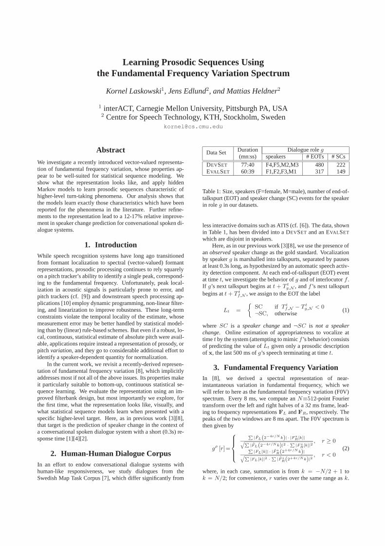
Figure 1: A sample fundamental frequency variation spectrum;thex−axis represents change in octaves per 8 ms.

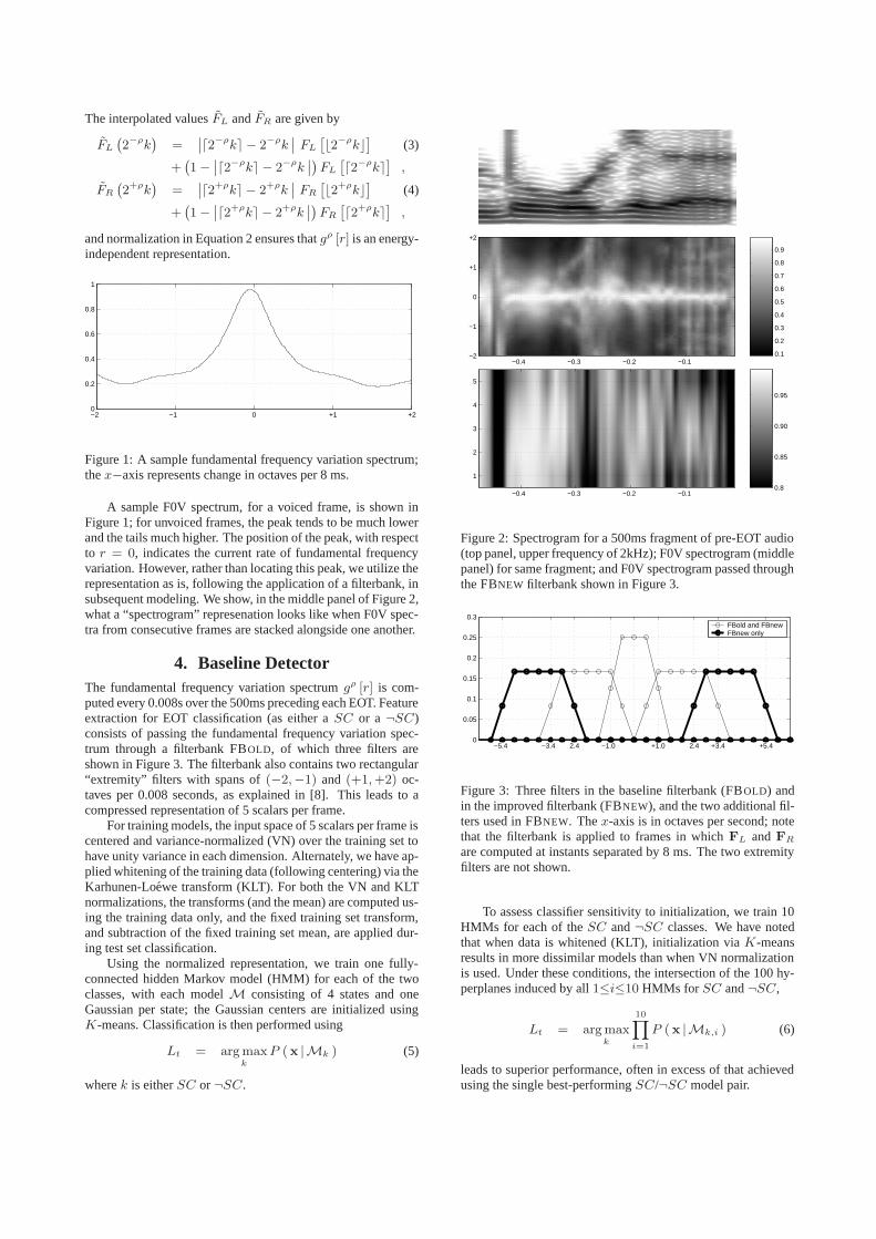
A sample F0V spectrum, for a voiced frame, is shown inFigure 1; for unvoiced frames, the peak tends to be much lowerand the tails much higher. The position of the peak, with respectto r = 0, indicates the current rate of fundamental frequencyvariation. However, rather than locating this peak, we utilize therepresentation as is, following the application of a filterbank, insubsequent modeling. We show, in the middle panel of Figure 2,what a “spectrogram” represenation looks like when F0V spec-tra from consecutive frames are stacked alongside one another.

4. Baseline DetectorThe fundamental frequency variation spectrumgρ [r] is com-puted every 0.008s over the 500ms preceding each EOT. Featureextraction for EOT classification (as either aSC or a ¬SC)consists of passing the fundamental frequency variation spec-trum through a filterbank FBOLD, of which three filters areshown in Figure 3. The filterbank also contains two rectangular“extremity” filters with spans of(−2,−1) and (+1, +2) oc-taves per 0.008 seconds, as explained in [8]. This leads to acompressed representation of 5 scalars per frame.

For training models, the input space of 5 scalars per frame iscentered and variance-normalized (VN) over the training set tohave unity variance in each dimension. Alternately, we have ap-plied whitening of the training data (following centering) via theKarhunen-Loewe transform (KLT). For both the VN and KLTnormalizations, the transforms (and the mean) are computed us-ing the training data only, and the fixed training set transform,and subtraction of the fixed training set mean, are applied dur-ing test set classification.

Using the normalized representation, we train one fully-connected hidden Markov model (HMM) for each of the twoclasses, with each modelM consisting of 4 states and oneGaussian per state; the Gaussian centers are initialized usingK-means. Classification is then performed using

Lt = arg maxk

P (x |Mk ) (5)

wherek is eitherSC or¬SC.

0.1

0.2

0.3

0.4

0.5

0.6

0.7

0.8

0.9

−0.4 −0.3 −0.2 −0.1−2

−1

0

+1

+2

0.8

0.85

0.90

0.95

−0.4 −0.3 −0.2 −0.1

1

2

3

4

5

Figure 2: Spectrogram for a 500ms fragment of pre-EOT audio(top panel, upper frequency of 2kHz); F0V spectrogram (middlepanel) for same fragment; and F0V spectrogram passed throughthe FBNEW filterbank shown in Figure 3.

−5.4 −3.4 2.4 −1.0 +1.0 2.4 +3.4 +5.40

0.05

0.1

0.15

0.2

0.25

0.3FBold and FBnewFBnew only

Figure 3: Three filters in the baseline filterbank (FBOLD) andin the improved filterbank (FBNEW), and the two additional fil-ters used in FBNEW. Thex-axis is in octaves per second; notethat the filterbank is applied to frames in whichFL andFR

are computed at instants separated by 8 ms. The two extremityfilters are not shown.

To assess classifier sensitivity to initialization, we train 10HMMs for each of theSC and¬SC classes. We have notedthat when data is whitened (KLT), initialization viaK-meansresults in more dissimilar models than when VN normalizationis used. Under these conditions, the intersection of the 100 hy-perplanes induced by all1≤i≤10 HMMs for SC and¬SC,

Lt = arg maxk

10Y

i=1

P (x |Mk,i ) (6)

leads to superior performance, often in excess of that achievedusing the single best-performingSC/¬SC model pair.

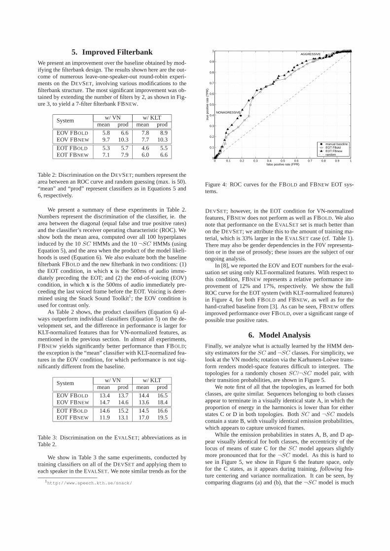
5. Improved FilterbankWe present an improvement over the baseline obtained by mod-ifying the filterbank design. The results shown here are the out-come of numerous leave-one-speaker-out round-robin experi-ments on the DEVSET, involving various modifications to thefilterbank structure. The most significant improvement was ob-tained by extending the number of filters by 2, as shown in Fig-ure 3, to yield a 7-filter filterbank FBNEW.

w/ VN w/ KLTSystemmean prod mean prod

EOV FBOLD 5.8 6.6 7.8 8.9EOV FBNEW 9.7 10.3 7.7 10.3

EOT FBOLD 5.3 5.7 4.6 5.5EOT FBNEW 7.1 7.9 6.0 6.6

Table 2: Discrimination on the DEVSET; numbers represent thearea between an ROC curve and random guessing (max. is 50).“mean” and “prod” represent classifiers as in Equations 5 and6, respectively.

We present a summary of these experiments in Table 2.Numbers represent the discrimination of the classifier, ie. thearea between the diagonal (equal false and true positive rates)and the classifier’s receiver operating characteristic (ROC). Weshow both the mean area, computed over all 100 hyperplanesinduced by the 10SC HMMs and the 10¬SC HMMs (usingEquation 5), and the area when the product of the model likeli-hoods is used (Equation 6). We also evaluate both the baselinefilterbank FBOLD and the new filterbank in two conditions: (1)the EOT condition, in whichx is the 500ms of audio imme-diately preceding the EOT; and (2) the end-of-voicing (EOV)condition, in whichx is the 500ms of audio immediately pre-ceeding the last voiced frame before the EOT. Voicing is deter-mined using the Snack Sound Toolkit1; the EOV condition isused for contrast only.

As Table 2 shows, the product classifiers (Equation 6) al-ways outperform individual classifiers (Equation 5) on the de-velopment set, and the difference in performance is larger forKLT-normalized features than for VN-normalized features, asmentioned in the previous section. In almost all experiments,FBNEW yields significantly better performance than FBOLD;the exception is the “mean” classifier with KLT-normalized fea-tures in the EOV condition, for which performance is not sig-nificantly different from the baseline.

w/ VN w/ KLTSystemmean prod mean prod

EOV FBOLD 13.4 13.7 14.4 16.5EOV FBNEW 14.7 14.6 13.6 18.4

EOT FBOLD 14.6 15.2 14.5 16.6EOT FBNEW 11.9 13.1 17.0 19.5

Table 3: Discrimination on the EVAL SET; abbreviations as inTable 2.

We show in Table 3 the same experiments, conducted bytraining classifiers on all of the DEVSET and applying them toeach speaker in the EVAL SET. We note similar trends as for the

1http://www.speech.kth.se/snack/

0 0.1 0.2 0.3 0.4 0.5 0.6 0.7 0.8 0.9 10

0.1

0.2

0.3

0.4

0.5

0.6

0.7

0.8

0.9

1

NONAGRESSIVE

AGGRESSIVE

false positive rate (FPR)

true

pos

itive

rat

e (T

PR

)

manual baselineEOT FBoldEOT FBnewrandom

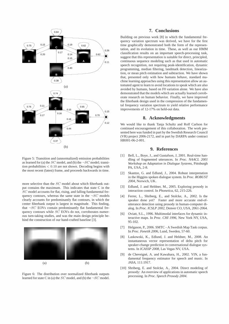
Figure 4: ROC curves for the FBOLD and FBNEW EOT sys-tems.

DEVSET; however, in the EOT condition for VN-normalizedfeatures, FBNEW does not perform as well as FBOLD. We alsonote that performance on the EVAL SET set is much better thanon the DEVSET; we attribute this to the amount of training ma-terial, which is 33% larger in the EVAL SET case (cf. Table 1).There may also be gender dependencies in the F0V representa-tion or in the use of prosody; these issues are the subject of ourongoing analysis.

In [8], we reported the EOV and EOT numbers for the eval-uation set using only KLT-normalized features. With respect tothis condition, FBNEW represents a relative performance im-provement of 12% and 17%, respectively. We show the fullROC curve for the EOT system (with KLT-normalized features)in Figure 4, for both FBOLD and FBNEW, as well as for thehand-crafted baseline from [3]. As can be seen, FBNEW offersimproved performance over FBOLD, over a significant range ofpossible true positive rates.

6. Model AnalysisFinally, we analyze what is actually learned by the HMM den-sity estimators for theSC and¬SC classes. For simplicity, welook at the VN models; rotation via the Karhunen-Loewe trans-form renders model-space features difficult to interpret. Thetopologies for a randomly chosenSC/¬SC model pair, withtheir transition probabilities, are shown in Figure 5.

We note first of all that the topologies, as learned for bothclasses, are quite similar. Sequences belonging to both classesappear to terminate in a visually identical state A, in which theproportion of energy in the harmonics is lower than for eitherstates C or D in both topologies. BothSC and¬SC modelscontain a state B, with visually identical emission probabilities,which appears to capture unvoiced frames.

While the emission probabilities in states A, B, and D ap-pear visually identical for both classes, the eccentricity of thelocus of means of state C for theSC model appears slightlymore pronounced that for the¬SC model. As this is hard tosee in Figure 5, we show in Figure 6 the feature space, onlyfor the C states, as it appears during training,following fea-ture centering and variance normalization. It can be seen, bycomparing diagrams (a) and (b), that the¬SC model is much

0.62

0.26

0.11

0.75

0.20

0.62

0.15

0.190.15

0.14

0.64

0.40

0.17

0.38

1

4

3

2A

C

D

B

(a)

0.11

0.74

0.650.15

0.16

0.17

0.76

0.16

0.44

0.37

0.12

0.15

0.70

A

B

D

C

4

3

1

2

(b)

Figure 5: Transition and (unnormalized) emission probabilitiesas learned for (a) theSC model, and (b) the¬SC model; transi-tion probabilities< 0.10 are not shown. Decoding begins withthe most recent (latest) frame, and proceeds backwards in time.

more selective than theSC model about which filterbank out-put contains the maximum. This indicates that state C in theSC model accounts for flat, rising, and falling fundamental fre-quency contours, whereas the same state in the¬SC modelsclearly accounts for predominantly flat contours, in which thecenter filterbank output is largest in magnitude. This finding,that ¬SC EOVs contain predominantly flat fundamental fre-quency contours whileSC EOVs do not, corroborates numer-ous turn-taking studies, and was the main design principle be-hind the construction of our hand-crafted baseline [3].

(a) (b)

Figure 6: The distribution over normalized filterbank outputslearned for state C in (a) theSC model, and (b) the¬SC model.

7. ConclusionsBuilding on previous work [8] in which the fundamental fre-quency variation spectrum was derived, we have for the firsttime graphically demonstrated both the form of the represen-tation, and its evolution in time. These, as well as our HMMclassification results on an important speech-processing task,suggest that this representation is suitable for direct, principled,continuous sequence modeling such as that used in automaticspeech recognition, not requiring peak-identification, dynamicprogramming, median filtering, landmark detection, lineariza-tion, or mean pitch estimation and subtraction. We have shownthat, presented only with how humans behave, standard ma-chine learning approaches using this representation allow an au-tomated agent to learn to avoid locations to speak which are alsoavoided by humans, based on F0 variation alone. We have alsodemonstrated that the models which are actually learned corrob-orate research on human behavior. Finally, we have improvedthe filterbank design used in the compression of the fundamen-tal frequency variation spectrum to yield relative performanceimprovements of 12-17% on held-out data.

8. AcknowledgmentsWe would like to thank Tanja Schultz and Rolf Carlson forcontinued encouragement of this collaboration. The work pre-sented here was funded in part by the Swedish Research Council(VR) project 2006-2172, and in part by DARPA under contractHR001-06-2-001.

9. References[1] Bell, L., Boye, J., and Gustafson, J, 2001. Real-time han-

dling of fragmented utterances. InProc. NAACL 2001Workshop on Adaptation in Dialogue Systems, PittsburghPA, USA, 2-8.

[2] Skantze, G. and Edlund, J., 2004. Robust interpretationin the Higgins spoken dialogue system. InProc. ROBUST2004, Norwich, UK.

[3] Edlund, J. and Heldner, M., 2005. Exploring prosody ininteraction control. InPhonetica, 62, 215-226.

[4] Ferrer, L., Shriberg, E., and Stolcke, A., 2002. Is thespeaker done yet? Faster and more accurate end-of-utterance detection using prosody in human-computer di-alog. InProc. ICSLP 2002, Denver CO, USA, 2061-2064.

[6] Oviatt, S.L., 1996. Multimodal interfaces for dynamic in-teractive maps. InProc. CHI 1996, New York NY, USA,95-102.

[7] Helgason, P., 2006. SMTC - A Swedish Map Task corpus.In Proc. Fonetik 2006, Lund, Sweden, 57-60.

[8] Laskowski, K., Edlund, J. and Heldner, M., 2008. Aninstantaneous vector representation of delta pitch forspeaker-change prediction in conversational dialogue sys-tems. InICASSP 2008, Las Vegas NV, USA.

[9] de Cheveigne, A. and Kawahara, H., 2002. YIN, a fun-damental frequency estimator for speech and music. InJASA, 111:1917.

[10] Shriberg, E. and Stolcke, A., 2004. Direct modeling ofprosody: An overview of applications in automatic speechprocessing. InProc. Speech Prosody 2004.