learning representation & behavior - umass...

June 25, 2006 ICML 2006 Tutorial

Learning Representation & Behavior:Manifold and Spectral Methods for

Markov Decision Processes and Reinforcement Learning

Sridhar Mahadevan, U. Mass, Amherst

Mauro Maggioni, Yale Univ.

http://www.math.yale.edu/~mmm82/MM_Snapshot.jpg


Outline

• Part One– History and Motivation (9:00-9:15)– Overview of framework (9:15-9:30)– Technical Background (9:30-10:30)– Questions: (10:30-10:45)

• Part Two– Algorithms and implementation (11:15-11:45)– Experimental Results (11:45-12:30)– Discussion and Future Work (12:30-12:45)– Questions (12:45-1:00)


Mathematical Foundations

• What we will assume:– Basic knowledge of machine learning, Markov

decision processes and reinforcement learning– Linear algebra , graph theory, and statistics

• What we will introduce:– Least squares techniques (for solving MDPs)– Spectral graph theory: matrices graphs– Fourier and wavelet bases on graphs– Continuous manifolds


Tutorial Decomposition

• Sridhar Mahadevan– History and motivation– Overview of the framework– Fourier (Laplacian) approach: global bases

• Mauro Maggioni– Harmonic analysis on graphs and manifolds– Diffusion wavelets: local bases

• Both:– Algorithms, experiments, implementation– Future work


Outline




Credit Assignment Problem (Minsky, Steps Toward AI, 1960)

States

Tasks

Time

s

s’

r

Challenge: Need a unified approach to the credit assignment problem


Samuel’s Checker Player

(Arthur Samuel, 1950s)• Samuel’s work laid the

foundations for many later ideas: temporal-difference learning, parametric function approximation, evaluation functions,…

• However, his work did not address a crucial problem: learning of representation


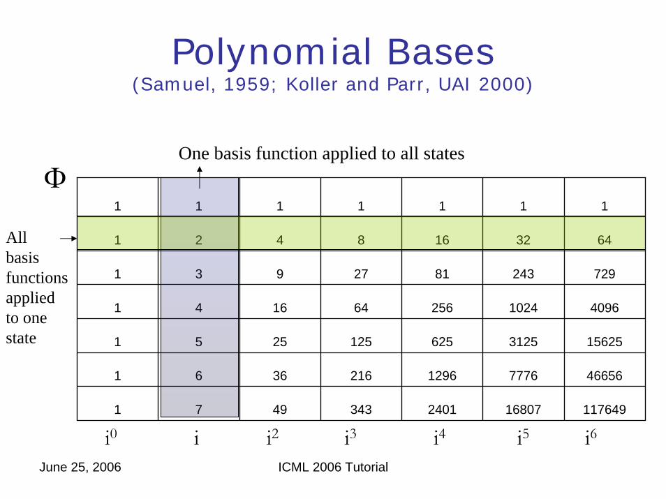
Polynomial Bases(Samuel, 1959; Koller and Parr, UAI 2000)

1 1 1 1 1 1 1

1 2 4 8 32 6416

1 3 9 27 81 243 729

1 4 16 64 256 1024 4096

1 5 25 125 625 3125 15625

1 6 36 216 1296 7776 46656

1 7 49 343 2401 16807 117649

One basis function applied to all states

Allbasisfunctionsappliedto onestate

i0 i i2 i3 i4 i5 i6

Φ


How to find a good basis?

1 2

3 4

5 6

7

Goal

Any function on this graphis a vector in R7

The question we want to ask ishow to construct a basis set forapproximating functions on this graph

Solution 1: use the unit basisSolution 2: use polynomials or RBFs

Neither of these exploit geometrye1 = [1, …, 0]ei = [0, …, i, …,0]


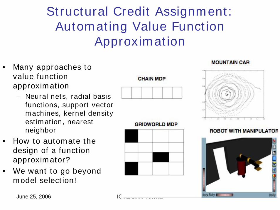
Structural Credit Assignment: Automating Value Function

Approximation

• Many approaches to value function approximation– Neural nets, radial basis

functions, support vector machines, kernel density estimation, nearest neighbor

• How to automate the design of a function approximator?

• We want to go beyond model selection!


Standard Approaches to VFACan Easily Fail!

(Dayan, Neural Comp, 1993; Drummond, JAIR 2003)

0

10

20

05

1015

200

20

40

60

80

100

Optimal Value Function

05

1015

20

0

10

200

10

20

30

Value Function Approximation using Polynomials

05

1015

20

0

10

200

20

40

60

80

Value Function Approximation using Radial Basis Functions

OPTIMAL VF POLYNOMIAL RADIAL BASIS FUNCTIONMulti-roomenvironment

G These approaches measure distancesin ambient space, not on the manifold!


Learning Representations by Global State Space Analysis

(Saul Amarel, 1960s) Missionaries and Cannibal

Find symmetries and bottlenecks in state spaces


Outline




-2 -1.5 -1 -0.5 0 0.5 1 1.5 2-8

-6

-4

-2

0

2

4

6

8 Fourier

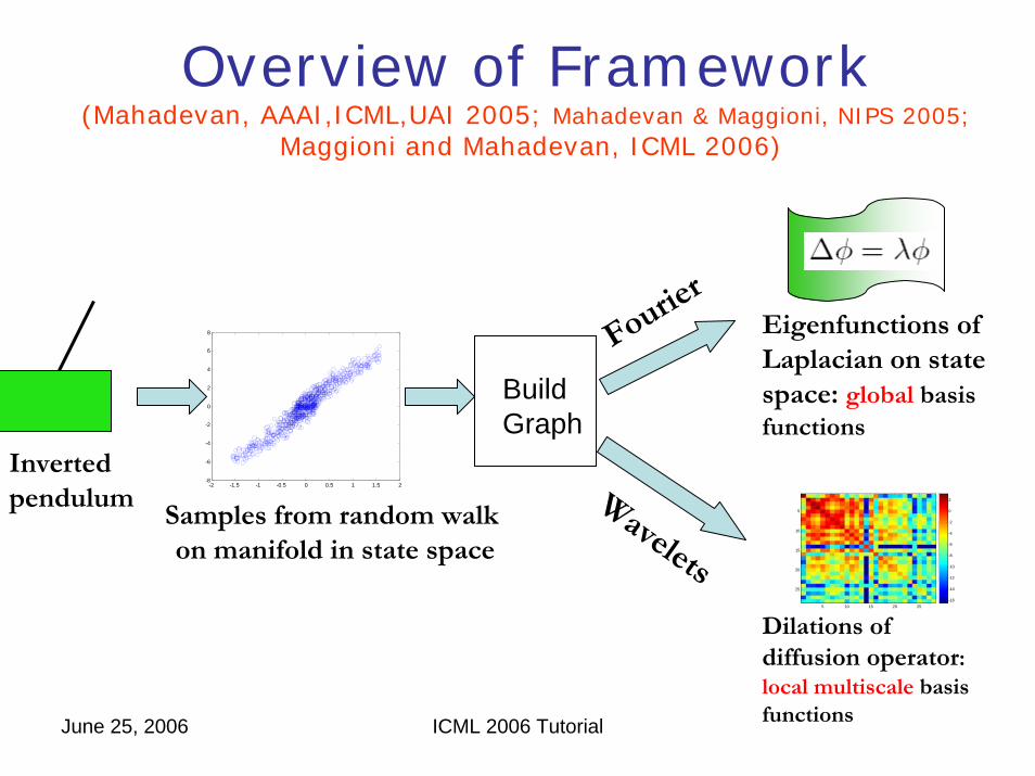
Samples from random walkon manifold in state space

Wavelets

Inverted pendulum

5 10 15 20 25

5

10

15

20

25

-16

-14

-12

-10

-8

-6

-4

-2

0

2

Eigenfunctions ofLaplacian on statespace: global basis functions

Dilations ofdiffusion operator:local multiscale basis functions

Overview of Framework(Mahadevan, AAAI,ICML,UAI 2005; Mahadevan & Maggioni, NIPS 2005;

Maggioni and Mahadevan, ICML 2006)

BuildGraph


Proto-Value Functions(Mahadevan: AAAI 2005, ICML 2005, UAI 2005)

Proto-value functions are reward-independentglobal (or local) basis functions, customizedto a state (action) space


Value Function Approximation using Fourier and Wavelet Bases

0

10

20

05

1015

200

20

40

60

80

100


OPTIMAL VF FOURIER BASIS0

5

10

15

20

05

1015

200

20

40

60

Value function approximation using diffusion wavelets

WAVELET BASIS

These bases are automatically learnedfrom a set of transitions (s,a,s’)

0

10

20

05101520-20

0

20

40

60

80

Value Function Approximation using Laplacian Eigenfunctions


Laplacian Proto-Value Functions: Inverted Pendulum


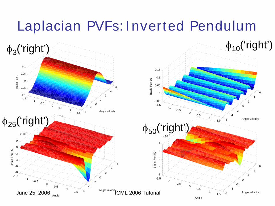
Laplacian PVFs:Inverted Pendulum

-1.5-1

-0.50

0.51

1.5 -6-4

-20

24

6

-0.1

-0.05

0

0.05

0.1

Angle velocity

Angle

Bas

is F

cn 3

-1.5-1

-0.50

0.51

1.5 -6-4

-20

24

6

-0.05

0

0.05

0.1

0.15

Angle velocity

Angle

Bas

is F

cn 1

0

-1.5-1

-0.50

0.51

1.5 -6-4

-20

24

6

-8

-6

-4

-2

0

2

x 10-3

Angle velocity

Angle

Bas

is F

cn 2

5

-1.5-1

-0.50

0.51

1.5 -6-4

-20

24

6

-6

-4

-2

0

2

x 10-3

Angle velocity

Angle

Bas

is F

cn 5

0

φ10(‘right’)

φ50(‘right’)

φ3(‘right’)

φ25(‘right’)


Laplacian Proto-Value Functions:Mountain Car


-1.5-1

-0.50

0.51 -0.1

-0.05

0

0.05

0.1

-0.04

-0.02

0

0.02

0.04

0.06

Velocity

Position

Bas

is F

cn 2

5

-1.5-1

-0.50

0.51 -0.1

-0.05

0

0.05

0.1

-0.04

-0.02

0

0.02

0.04

Velocity

Position

Bas

is F

cn 3

Laplacian PVFs: Mountain Carφ3(‘reverse’) φ5(‘reverse’)

φ25(‘reverse’)φ40(‘reverse’)

-1.5-1

-0.50

0.51 -0.1

-0.05

0

0.05

0.1

-0.04

-0.02

0

0.02

0.04

Velocity

Position

Bas

is F

cn 5

-1.5-1

-0.50

0.51 -0.1

-0.05

0

0.05

0.1

-0.05

0

0.05

0.1

0.15

Velocity

Position

Bas

is F

cn 4

0


Multiresolution Manifold Learning

• Fourier methods, like Laplacian manifold or spectral learning, rely on eigenvectors– Eigenvectors are useful in analyzing long-term global

behavior of a system (e.g, PageRank)– They are rather poor at short or medium term transient

analysis (or locally discontinuities)

• Wavelet methods [Daubechies, Mallat]– Inherently multi-resolution analysis– Local basis functions with compact support

• Diffusion wavelets [Coifman and Maggioni, 2004]– Extend classical wavelets to graphs and manifolds


Multiscale Analysis: Diffusion Wavelet Bases(Coifman and Maggioni, 2004; Mahadevan and Maggioni, NIPS 2005)

Level 2 Level 3

Level 4 Level 5

δ functions → Global eigenvectors


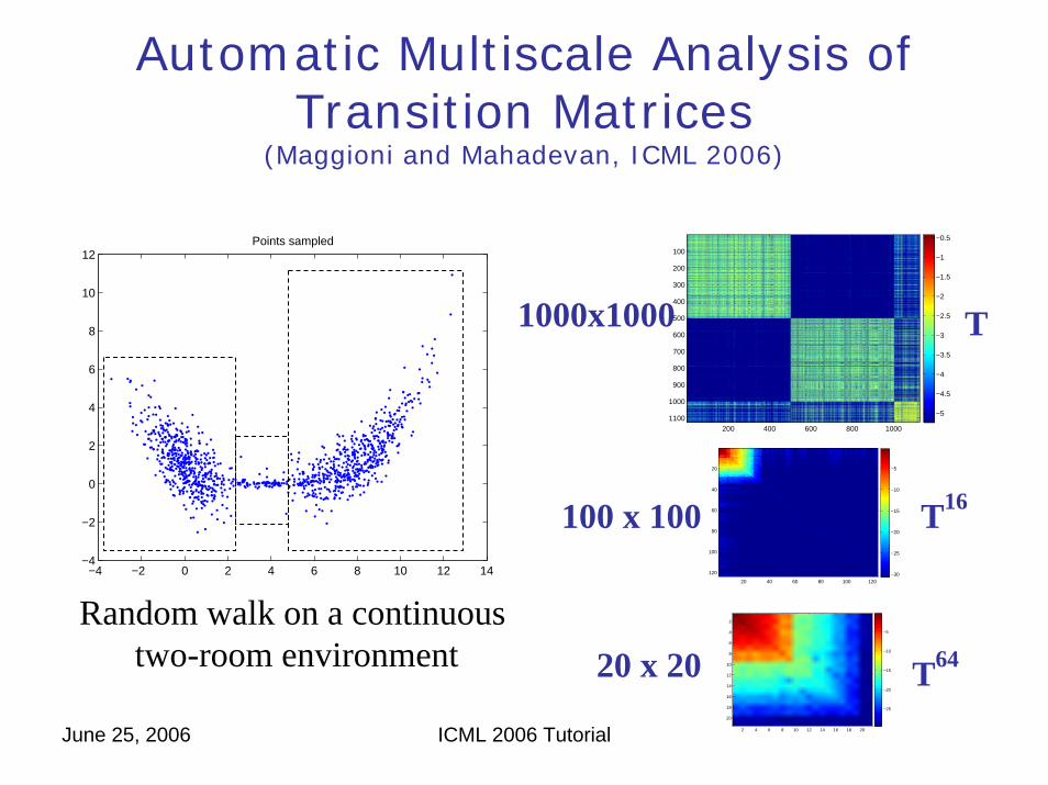
Automatic Multiscale Analysis of Transition Matrices

(Maggioni and Mahadevan, ICML 2006)

−4 −2 0 2 4 6 8 10 12 14−4

−2

0

2

4

6

8

10

12Points sampled

200 400 600 800 1000

100

200

300

400

500

600

700

800

900

1000

1100−5

−4.5

−4

−3.5

−3

−2.5

−2

−1.5

−1

−0.5

20 40 60 80 100 120

20

40

60

80

100

120 −30

−25

−20

−15

−10

−5

2 4 6 8 10 12 14 16 18 20

2

4

6

8

10

12

14

16

18

20

−25

−20

−15

−10

−5

1000x1000

100 x 100

Random walk on a continuous two-room environment 20 x 20

T

T16

T64


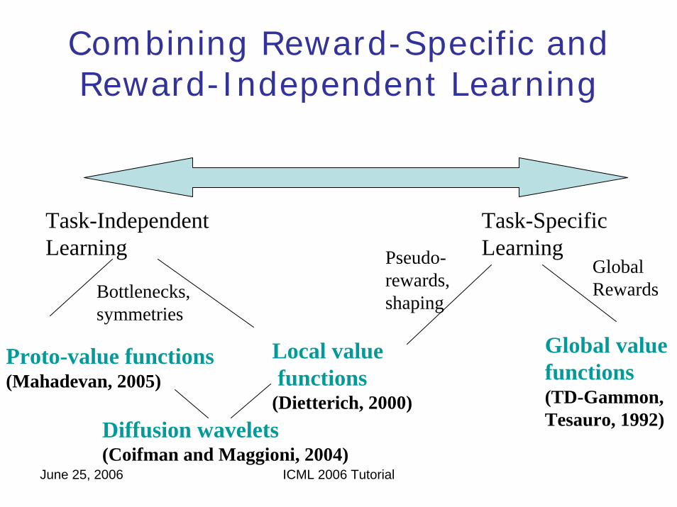
Combining Reward-Specific and Reward-Independent Learning

Task-IndependentLearning

Task-SpecificLearning

Global value functions(TD-Gammon,Tesauro, 1992)

Proto-value functions(Mahadevan, 2005)

GlobalRewards

Local valuefunctions

(Dietterich, 2000)

Pseudo-rewards,shapingBottlenecks,

symmetries

Diffusion wavelets(Coifman and Maggioni, 2004)


Learning Representation and Behavior

• Unified framework for credit assignment problem:– Harmonic analysis on graphs and manifolds– Fourier and wavelet bases (for value functions,

transition matrices, policies, and more…)– Unifies RL with manifold and spectral learning

• Novel representations and algorithms:– Automatic basis function construction (values, policies)– Representation Policy iteration with an adaptive basis– Multiscale diffusion policy evaluation – A new representation for temporally extended actions – Transfer learning by representation sharing– Extendable to POMDPs and PSRs


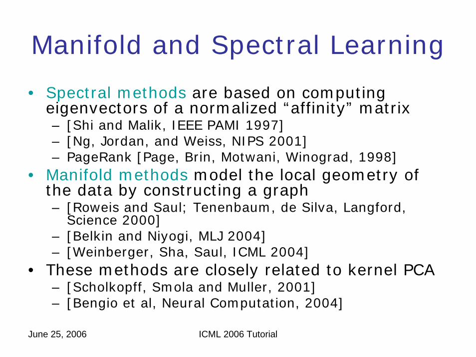
Manifold and Spectral Learning

• Spectral methods are based on computing eigenvectors of a normalized “affinity” matrix– [Shi and Malik, IEEE PAMI 1997]– [Ng, Jordan, and Weiss, NIPS 2001] – PageRank [Page, Brin, Motwani, Winograd, 1998]

• Manifold methods model the local geometry of the data by constructing a graph– [Roweis and Saul; Tenenbaum, de Silva, Langford,

Science 2000]– [Belkin and Niyogi, MLJ 2004]– [Weinberger, Sha, Saul, ICML 2004]

• These methods are closely related to kernel PCA– [Scholkopff, Smola and Muller, 2001]– [Bengio et al, Neural Computation, 2004]


“Curse of Dimensionality”

• Two active subfields in machine learning– Learning in inner product spaces: kernel methods– Manifold learning: nonlinear dimensionality reduction

• Fourier and wavelet bases on graphs– Based on analysis of the heat kernel of a graph– Basis for Hilbert space of functions on a graph– Nonlinear low-dimensional embedding of the graph

• Measure distances “intrinsically” in data space, not in ambient space!– Distance is based on diffusions (heat flow)– Closely connected to random walks on graphs


Outline




Finite State Probabilistic Models

Markov Chain

1

2

3

.3.7

.4

.6

1

2

3

Markov Decision Process

+3 +5

-1

-2

+6

0

12

23

Hidden Markov Model

31

.3.7

.4

.6

Partially Observable Markov Decision Process

11

2

23

3

+3+5

-1

0

+6

-2

How to learnmulti-scalerepresentations foranalysis usingthese models?


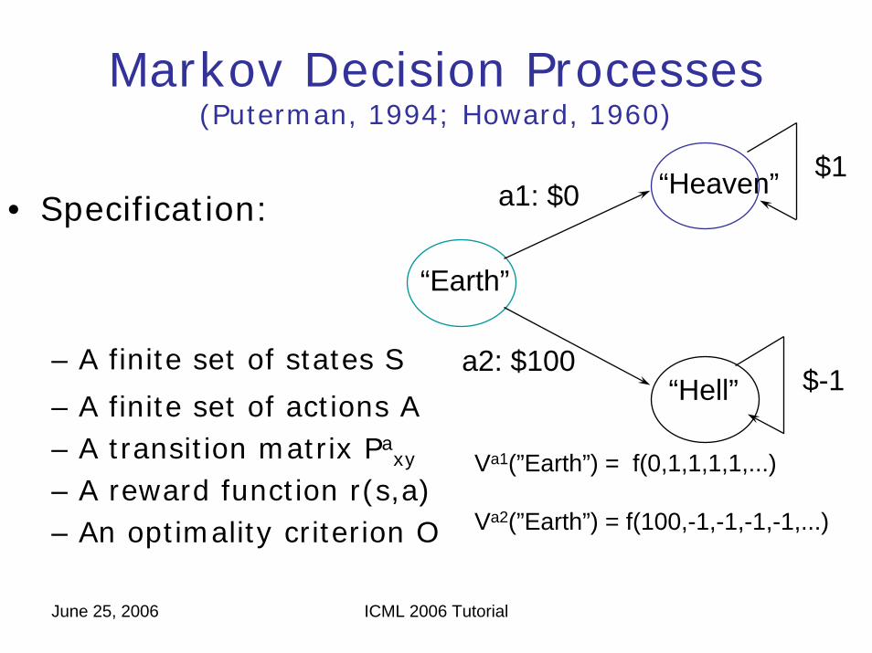
Markov Decision Processes(Puterman, 1994; Howard, 1960)

• Specification:

– A finite set of states S

– A finite set of actions A– A transition matrix Pa

xy

– A reward function r(s,a)– An optimality criterion O

“Earth”

“Heaven”

“Hell”

$1

$-1

a1: $0

a2: $100

Va1(”Earth”) = f(0,1,1,1,1,...)

Va2(”Earth”) = f(100,-1,-1,-1,-1,...)


Graded myopia: “discounted sum of rewards”Maximize

Hell if γ < 0.98, otherwise HeavenMaximize “average-adjusted sum of rewards”

Always go to heaven!

γ ttt

r∑

limn

r

ntt

n

→ ∞=∑

1

Infinite Horizon Markov Decision Processes


Bellman Optimality Equation

-1

Choosegreedy actiongiven V*

4 23

-1

10 49 100

Goal!

+50

EXIT EAST

EXIT WEST

WAIT


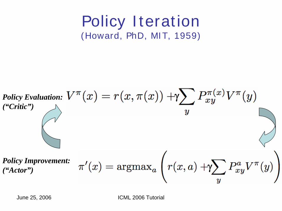
Policy Iteration(Howard, PhD, MIT, 1959)

Policy Improvement:(“Actor”)

Policy Evaluation:(“Critic”)

γ

γ


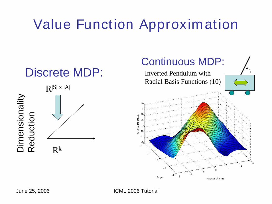
Value Function Approximation

Inverted Pendulum withRadial Basis Functions (10)

R|S| x |A|

RkDim

ensi

onal

ityR

educ

tion

Discrete MDP:Continuous MDP:


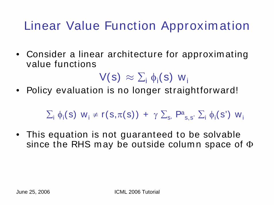
Linear Value Function Approximation

• Consider a linear architecture for approximating value functions

V(s) ≈ ∑i φi(s) wi• Policy evaluation is no longer straightforward!

∑i φi(s) wi ≠ r(s,π(s)) + γ ∑s’Pa

s,s’ ∑i φi(s’) wi

• This equation is not guaranteed to be solvable since the RHS may be outside column space of Φ


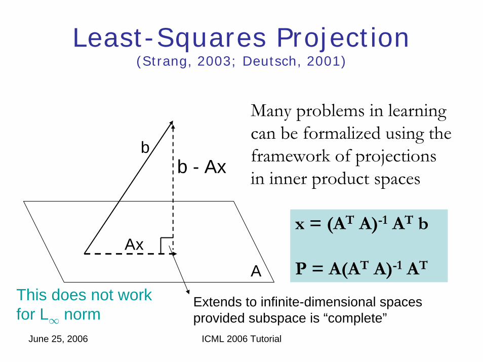
Least-Squares Projection(Strang, 2003; Deutsch, 2001)

b

Ax

A

Many problems in learningcan be formalized using theframework of projectionsin inner product spaces

x = (AT A)-1 AT b

P = A(AT A)-1 AT

b - Ax

Extends to infinite-dimensional spacesprovided subspace is “complete”

This does not workfor L∞ norm


Bellman Residual Method(Munos, ICML 03; Lagoudakis and Parr, JMLR 03)

• Let us write the Bellman equation in matrix form as

Φ wπ ≈ Rπ + γ Pπ Φ wπ

• Collecting the terms, we rewrite this as(Φ - γ Pπ Φ) wπ ≈ Rπ

• The least-squares solution is wπ = [(Φ - γ Pπ Φ)T (Φ - γ Pπ Φ)]-1 (Φ - γ Pπ Φ)T Rπ


Bellman Residual Method

∑=i

ii wssV )()(ˆ φ

Subspace Φ(RBF, polynomials, Fourier or wavelet

bases)

))(ˆ( sVT π

Min

imiz

e R

esid

ual


Bellman Fixpoint Method

• Another way to obtain a least-squares solution is to project the backed-up value function Tπ(Vπ)

P = Φ (ΦT Φ)-1 ΦT

• The least-squares projected weights then becomes

Wπ = (ΦT Φ)-1 ΦT [Rπ + γ Pπ Vπ]


Bellman Fixpoint Method

∑=i

ii wssV )()(ˆ φ

Subspace Φ(RBF, polynomials, Fourier or wavelet

bases)

))(ˆ( sVT π

Minimize Projected Resid

ual


-2 -1.5 -1 -0.5 0 0.5 1 1.5 2-8

-6

-4

-2

0

2

4

6

8 Fourier


Wavelets

Inverted pendulum

5 10 15 20 25

5

10

15

20

25

-16

-14

-12

-10

-8

-6

-4

-2

0

2





BuildGraph


Graph Adjacency Matrix

1 2

3 4

5 6

7

Goal

Adjacency Matrix

0 1 1 0 0 0 0

1 0 0 1 0 0 0

1 0 0 1 1 0 0

0 1 1 0 0 1 1

0 0 1 0 0 1 0

0 0 0 1 1 0 0

0 0 0 1 0 0 0


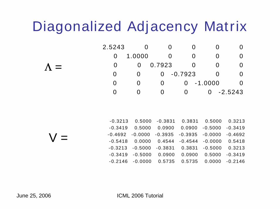
Spectral Theorem

• From basic linear algebra, we know that since the adjacency matrix A is symmetric, we can use the spectral theorem

A = V Λ VT

• V is a matrix of orthonormal eigenvectors, Λ is a diagonal matrix of eigenvalues

• Eigenvectors satisfy the following property:

A x = λ x


Diagonalized Adjacency Matrix2.5243 0 0 0 0 0

0 1.0000 0 0 0 00 0 0.7923 0 0 00 0 0 -0.7923 0 00 0 0 0 -1.0000 00 0 0 0 0 -2.5243

Λ =

-0.3213 0.5000 -0.3831 0.3831 0.5000 0.3213-0.3419 0.5000 0.0900 0.0900 -0.5000 -0.3419-0.4692 -0.0000 -0.3935 -0.3935 -0.0000 -0.4692-0.5418 0.0000 0.4544 -0.4544 -0.0000 0.5418-0.3213 -0.5000 -0.3831 0.3831 -0.5000 0.3213-0.3419 -0.5000 0.0900 0.0900 0.5000 -0.3419-0.2146 -0.0000 0.5735 0.5735 0.0000 -0.2146

V =


Inner Product Spaces

• An inner product space is a vector space associated with an inner product (e.g, Rn)

• The set of all functions Φ on a graph G = (V, E) forms an inner product space, where the inner product is defined as

<f , g> = ∑i f(i) g(i) • An operator O on an inner product space of functions is a

mapping O: Φ → Φ


Adjacency Operator

• Let us now revisit the adjacency matrix and treat it as an operator

• What is its effect on functions on the graph?

• It is easy to see that

A f(i) = ∑j ~ i f(j)

0 1 1 0 0 0 0

1 0 0 1 0 0 0

1 0 0 1 1 0 0

0 1 1 0 0 1 1

0 0 1 0 0 1 0

0 0 0 1 1 0 0

0 0 0 1 0 0 0


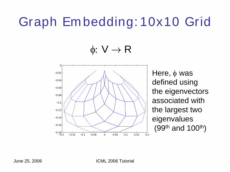
Graph Embedding:10x10 Grid

−0.2 −0.15 −0.1 −0.05 0 0.05 0.1 0.15 0.2−0.18

−0.16

−0.14

−0.12

−0.1

−0.08

−0.06

−0.04

−0.02

0

φ: V → R

Here, φ wasdefined usingthe eigenvectorsassociated withthe largest twoeigenvalues(99th and 100th)


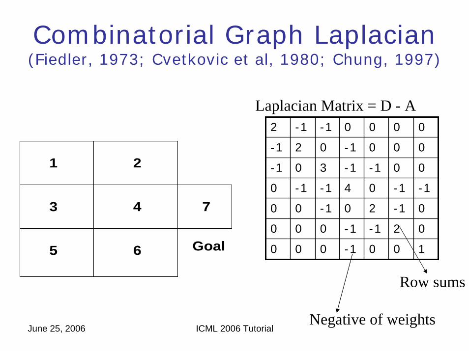
Combinatorial Graph Laplacian (Fiedler, 1973; Cvetkovic et al, 1980; Chung, 1997)

1 2

3 4

5 6

7

Goal

Laplacian Matrix = D - A 2 -1 -1 0 0 0 0

-1 2 0 -1 0 0 0

-1 0 3 -1 -1 0 0

0 -1 -1 4 0 -1 -1

0 0 -1 0 2 -1 0

0 0 0 -1 -1 2 0

0 0 0 -1 0 0 1

Row sums

Negative of weights


One-Dimensional Chain MDP

504

5

closedchain

1 2 3

4

5

67

0 50−0.2

0

0.2

0 50−0.2

0

0.2

0 50−0.2

0

0.2

0 50−0.2

0

0.2

0 50−0.2

0

0.2

0 50−0.2

0

0.2

0 50−0.2

0

0.2

0 50−0.2

0

0.2

0 50−0.2

0

0.2

0 50

0.1414

Eigenvectors of the Graph Laplacian


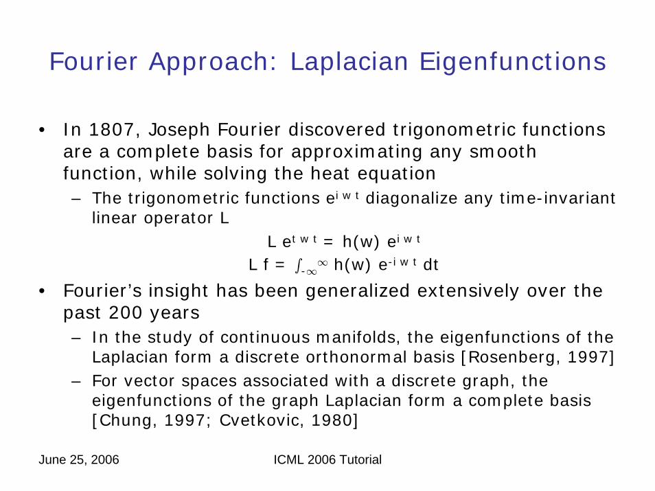
Fourier Approach: Laplacian Eigenfunctions

• In 1807, Joseph Fourier discovered trigonometric functions are a complete basis for approximating any smooth function, while solving the heat equation– The trigonometric functions ei w t diagonalize any time-invariant

linear operator LL et w t = h(w) ei w t

L f = ∫-∞∞ h(w) e-i w t dt

• Fourier’s insight has been generalized extensively over the past 200 years– In the study of continuous manifolds, the eigenfunctions of the

Laplacian form a discrete orthonormal basis [Rosenberg, 1997]– For vector spaces associated with a discrete graph, the

eigenfunctions of the graph Laplacian form a complete basis [Chung, 1997; Cvetkovic, 1980]


Simple Properties of the Laplacian

• The Laplacian is positive semidefinite

• The Laplacian for this graph is [1 -1; -1 1]• Note that xT L x = (x1 – x2)2

• We can express the Laplacian of any graph as the sum of the Laplacians of the same graph with all edges deleted, except for one.

• This implies that <x, Lx> = xT L x = ∑u ∼ v (xu – xv)2


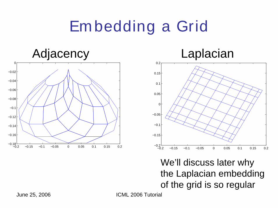
Embedding a Grid

−0.2 −0.15 −0.1 −0.05 0 0.05 0.1 0.15 0.2−0.18

−0.16

−0.14

−0.12

−0.1

−0.08

−0.06

−0.04

−0.02

0

−0.2 −0.15 −0.1 −0.05 0 0.05 0.1 0.15 0.2−0.2

−0.15

−0.1

−0.05

0

0.05

0.1

0.15

0.2

Adjacency Laplacian

We’ll discuss later whythe Laplacian embeddingof the grid is so regular


1 1.5 2 2.5 3 3.5 4 4.5 5-0.5

0

0.5

1

1.5

2

2.5

3

1 1.5 2 2.5 3 3.5 4 4.5 5-3

-2

-1

0

1

2

3

4

5

6

1 1.5 2 2.5 3 3.5 4 4.5 5-4

-3

-2

-1

0

1

2

3

4

5

6

1 1.5 2 2.5 3 3.5 4 4.5 5-4

-3

-2

-1

0

1

2

3

4

5

6

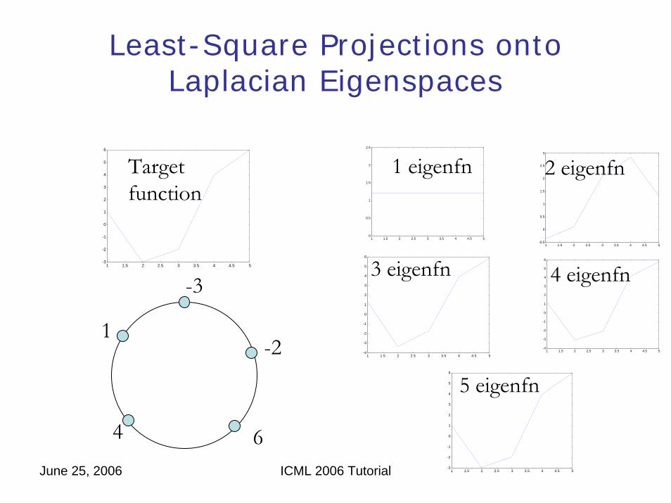
Least-Square Projections onto Laplacian Eigenspaces

1

-3

4 6

-2

1 1.5 2 2.5 3 3.5 4 4.5 5-3

-2

-1

0

1

2

3

4

5

6

1 1.5 2 2.5 3 3.5 4 4.5 50

0.5

1

1.5

2

2.5

Targetfunction

1 eigenfn 2 eigenfn

3 eigenfn 4 eigenfn

5 eigenfn


Laplacian vs. Polynomial Approximation on a Grid

0

5

10

0

5

100

50

100

150


0

5

10

0

5

100

20

40

60

80

100

Least-Squares Approximation using automatically learned Proto-Value Function

0 2 4 6 8 10 12 14 16 18 200

100

200

300

400

500

600

700

800MEAN-SQUARED ERROR OF LAPLACIAN vs. POLYNOMIAL STATE ENCODING

NUMBER OF BASIS FUNCTIONS

ME

AN

-SQ

UA

RE

D E

RR

OR

LAPLACIANPOLYNOMIAL

Numerical instabilityof polynomial basis


Linear Least-Squares Approximation with Laplacian Bases

0 5 10 15 20

010

20300

500

1000

The Target function

0 5 10 15 20

010

20300

500

1000

Reconstruction with 34 eigenfunctions

0 20 40 60 80 100 120 140 160 180 2000

1000

2000

3000

4000

5000

6000

7000

8000

9000

f’ = ∑i=1n <f, φi> φi

Leas

t-squ

ares

err

or

Number of basis functions


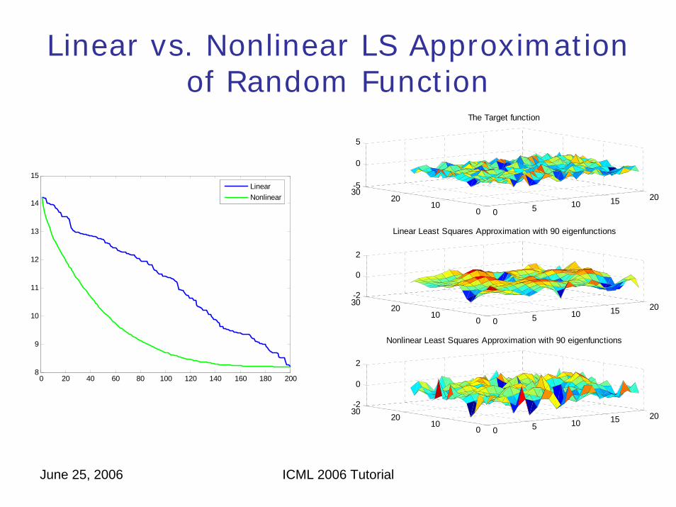
Linear vs. Nonlinear LS Approximation of Random Function

0 5 10 15 20

010

2030-5

0

5

The Target function

0 5 10 15 200

1020

30-2

0

2

Linear Least Squares Approximation with 90 eigenfunctions

0 5 10 15 200

1020

30-2

0

2

Nonlinear Least Squares Approximation with 90 eigenfunctions

0 20 40 60 80 100 120 140 160 180 2008

9

10

11

12

13

14

15LinearNonlinear


Graph Embedding• Consider the following optimization

problem mapping, where yi ∈ R is a mapping of the ith vertex to the real line

Minw ∑i,j (yi – yj)2 wi,j s.t. yT D y = 1• The best mapping is found by solving the

generalized eigenvector problemW φ = λ D φ

• If the graph is connected, this can be written as

D-1 W φ = λ φ


Normalized Graph Laplacian and Random Walks

• Given an undirected weighted graph G = (V, E, W), the random walk on the graph is defined by the transition matrix

P = D-1W– Random walk matrix is not symmetric

• Normalized Graph LaplacianL = D-1/2 (D - W) D-1/2 = I - D-1/2 W D-1/2

• The random walk matrix has the same eigenvalues as (I - L )

D-1W = D-1/2 (D-1/2 W D-1/2) D1/2 = D-1/2 (I - L ) D1/2


Operators on Graphs


Diffusion Analysis

• Fourier vs. wavelet analysis– Local vs. global analysis– Multiresolution modeling

• Diffusion wavelets [Coifman and Maggioni, 2004]

– Generalization of wavelets to graphs and manifolds– Provides a way to learn multiscale basis functions– Automatic hierarchical abstraction of Markov process on

graphs

1

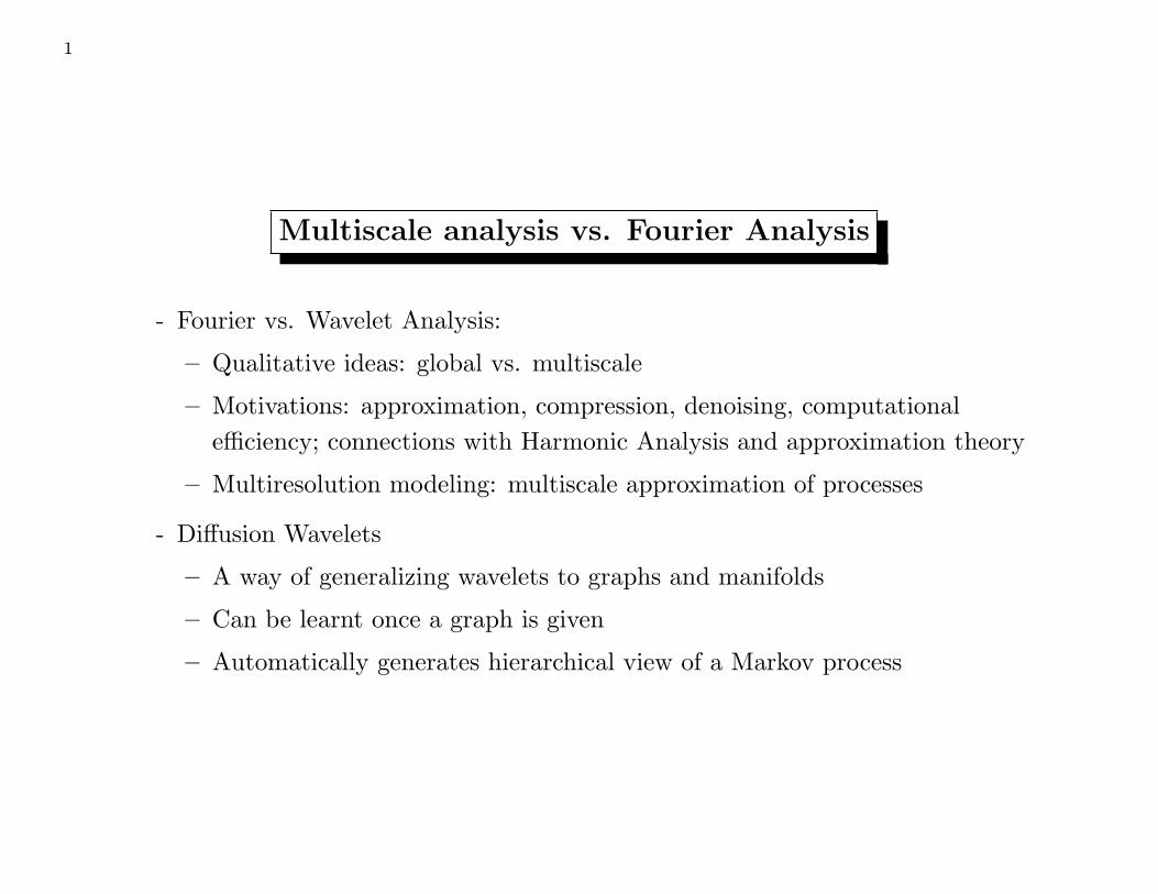
Multiscale analysis vs. Fourier Analysis

- Fourier vs. Wavelet Analysis:

– Qualitative ideas: global vs. multiscale

– Motivations: approximation, compression, denoising, computational

efficiency; connections with Harmonic Analysis and approximation theory

– Multiresolution modeling: multiscale approximation of processes

- Diffusion Wavelets

– A way of generalizing wavelets to graphs and manifolds

– Can be learnt once a graph is given

– Automatically generates hierarchical view of a Markov process

2

Qualitative ideas: multiscale vs. global

The setup is as before: we construct a set of basis functions adapted to the

geometry of the explored state space, and project a policy iteration algorithm in

a subspace spanned by those basis functions.

Instead of global Fourier-modes, we will use wavelet-like, multiscale basis

elements. They are also built from a diffusion operator T on a graph. We denote

them by φj,k, where j will indicate scale, and k location. These allow to

represent efficiently a broader class of functions than Fourier eigenfunctions, for

example functions which are piecewise smooth and not globally smooth.

This wavelet analysis is multiscale in at least three ways:

• in space: basis elements are localized, the elements at scale j have support of

roughly diameter δj , for some δ > 1;

• in frequency: basis elements at scale j have Fourier transform essentially

supported in [ǫ2−j

, ǫ2−j+1

];

• in time: it is possible to represent T 2j

on {φj,k}k by a small matrix, with

great precision.

3

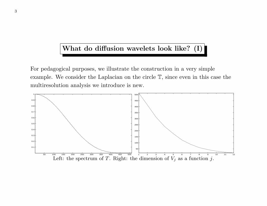
What do diffusion wavelets look like? (I)

For pedagogical purposes, we illustrate the construction in a very simple

example. We consider the Laplacian on the circle T, since even in this case the

multiresolution analysis we introduce is new.

50 100 150 200 250 300 350 400 450 500

0.1

0.2

0.3

0.4

0.5

0.6

0.7

0.8

0.9

1

1 2 3 4 5 6 7 8 9 10 11 12

50

100

150

200

250

300

350

400

450

500

Left: the spectrum of T . Right: the dimension of Vj as a function j.

4

50 100 150 200 250 300 350 400 450 500

−0.4

−0.2

0

0.2

0.4

0.6

50 100 150 200 250 300 350 400 450 500

−0.4

−0.3

−0.2

−0.1

0

0.1

0.2

0.3

0.4

0.5

50 100 150 200 250 300 350 400 450 500

−0.2

−0.15

−0.1

−0.05

0

0.05

0.1

0.15

0.2

0.25

0.3

50 100 150 200 250 300 350 400 450 500−0.08

−0.06

−0.04

−0.02

0

0.02

0.04

0.06

0.08

0.1

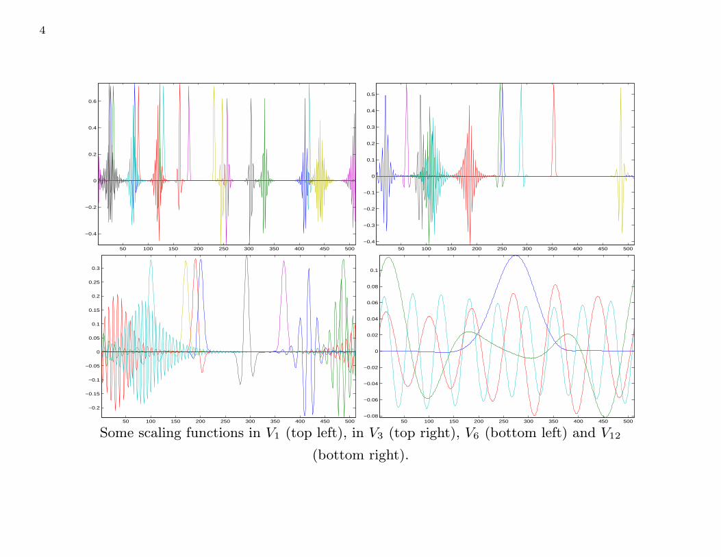
Some scaling functions in V1 (top left), in V3 (top right), V6 (bottom left) and V12

(bottom right).

5

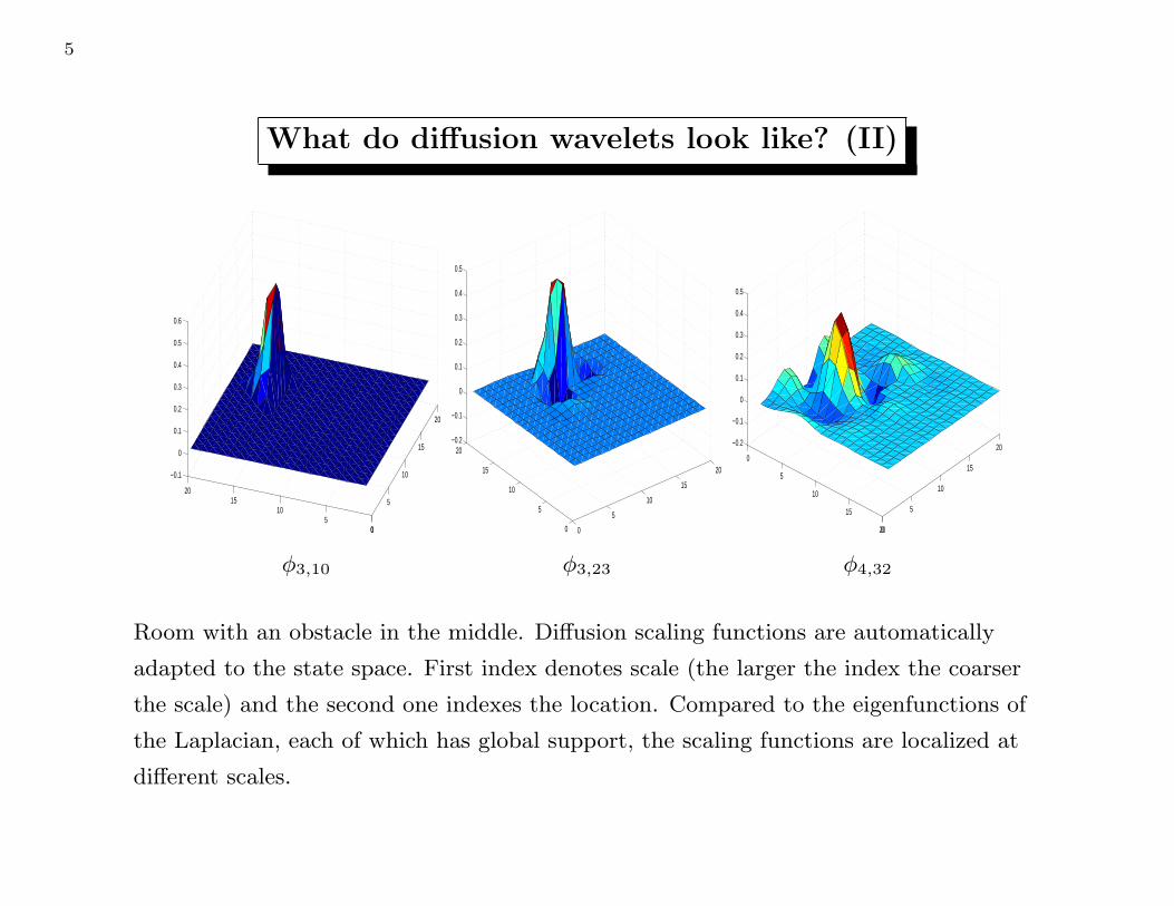
What do diffusion wavelets look like? (II)

0

5

10

15

20

05

1015

20

−0.1

0

0.1

0.2

0.3

0.4

0.5

0.6

φ3,10

0

5

10

15

20

0

5

10

15

20−0.2

−0.1

0

0.1

0.2

0.3

0.4

0.5

φ3,23

0

5

10

15

200

5

10

15

20−0.2

−0.1

0

0.1

0.2

0.3

0.4

0.5

φ4,32

Room with an obstacle in the middle. Diffusion scaling functions are automatically

adapted to the state space. First index denotes scale (the larger the index the coarser

the scale) and the second one indexes the location. Compared to the eigenfunctions of

the Laplacian, each of which has global support, the scaling functions are localized at

different scales.

6

0

5

10

15

20

0

5

10

15

20−0.1

−0.05

0

0.05

0.1

0.15

0.2

0.25

0.3

φ5,5

0

5

10

15

20

0

5

10

15

20−0.1

−0.05

0

0.05

0.1

0.15

0.2

0.25

φ6,8

0

5

10

15

20

0

5

10

15

20−0.06

−0.04

−0.02

0

0.02

0.04

0.06

0.08

0.1

0.12

φ9,2

7

What do diffusion wavelets look like? (III)

0

10

20

30

40

0

5

10

15

20

25

30−0.2

0

0.2

0.4

0.6

0.8

φ3,...

0

10

20

30

40

0

5

10

15

20

25

30−0.1

0

0.1

0.2

0.3

0.4

0.5

0.6

φ4,...

0

10

20

30

40

0

5

10

15

20

25

30−0.1

−0.05

0

0.05

0.1

0.15

0.2

0.25

0.3

0.35

φ5,...

0

10

20

30

40

0

5

10

15

20

25

30−0.02

0

0.02

0.04

0.06

0.08

0.1

φ8,...

Diffusion scaling functions on a discrete two-room spatial domain connected by a

common door. All the scaling functions are naturally adapted to the state space.

8

Connections with Harmonic Analysis, I

We need tools for efficiently working with functions on a manifold or graph: in

particular efficient and stable representation for functions of interest (e.g. value

functions). Assume a linear architecture:

f =∑

k

αkφk

where f is a function in the class of functions we want to approximate, φk’s are

basis functions (“building blocks” or “templates”), and the coefficients αk

contain the information for putting together the “building blocks” in order to

reconstruct (or approximate) f .

What does efficient mean? Few, in proportion to how “complicate” f is, and

efficiently-organized coefficients αk. Smoothness constraints become sparsity

constraints. For example, it is useful for linear approximation, that |αk| . k−γ .

Or, for nonlinear approximation, that |ασ(k)| . k−γ , for some permutation σ

(possibly σ(k) ≫ k!).

9

Connections with Harmonic Analysis, II

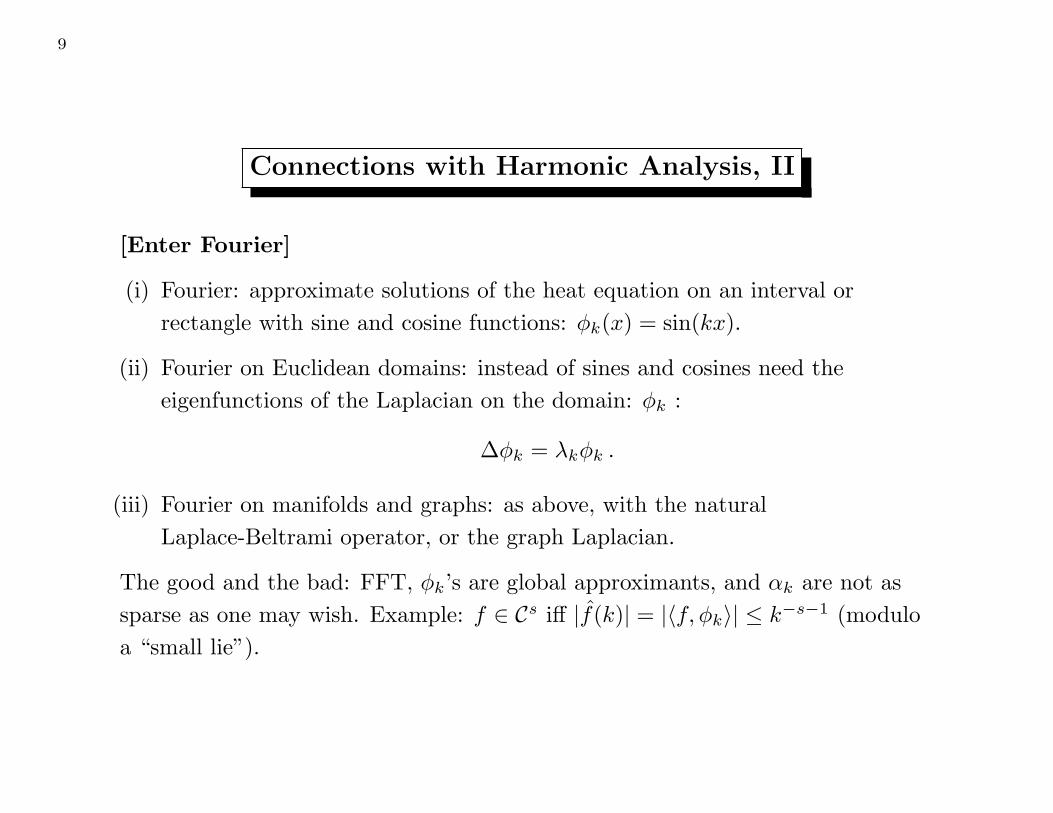
[Enter Fourier]

(i) Fourier: approximate solutions of the heat equation on an interval or

rectangle with sine and cosine functions: φk(x) = sin(kx).

(ii) Fourier on Euclidean domains: instead of sines and cosines need the

eigenfunctions of the Laplacian on the domain: φk :

∆φk = λkφk .

(iii) Fourier on manifolds and graphs: as above, with the natural

Laplace-Beltrami operator, or the graph Laplacian.

The good and the bad: FFT, φk’s are global approximants, and αk are not as

sparse as one may wish. Example: f ∈ Cs iff |f(k)| = |〈f, φk〉| ≤ k−s−1 (modulo

a “small lie”).

10

Connections with Harmonic Analysis, III

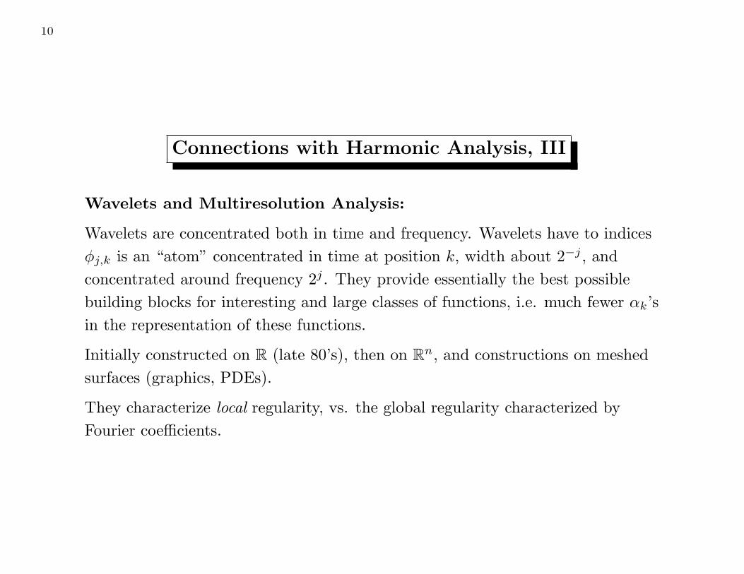
Wavelets and Multiresolution Analysis:

Wavelets are concentrated both in time and frequency. Wavelets have to indices

φj,k is an “atom” concentrated in time at position k, width about 2−j , and

concentrated around frequency 2j . They provide essentially the best possible

building blocks for interesting and large classes of functions, i.e. much fewer αk’s

in the representation of these functions.

Initially constructed on R (late 80’s), then on Rn, and constructions on meshed

surfaces (graphics, PDEs).

They characterize local regularity, vs. the global regularity characterized by

Fourier coefficients.

11

Example of nonlinear approximation

0

10

20

30

40

0

5

10

15

20

25

300

20

40

60

80

100

120

140

The Target function

True value function

10 20 30 40 50 60 70 80 90 100

−0.5

0

0.5

1

1.5

2 Best wavelet packet basisEigenfunction basis

Fourier and DWT nonlinear approx

0

10

20

30

40

0

5

10

15

20

25

30−5

0

5

10

15

20

25

30

35

Reconstruction with 30 eigenfunctions

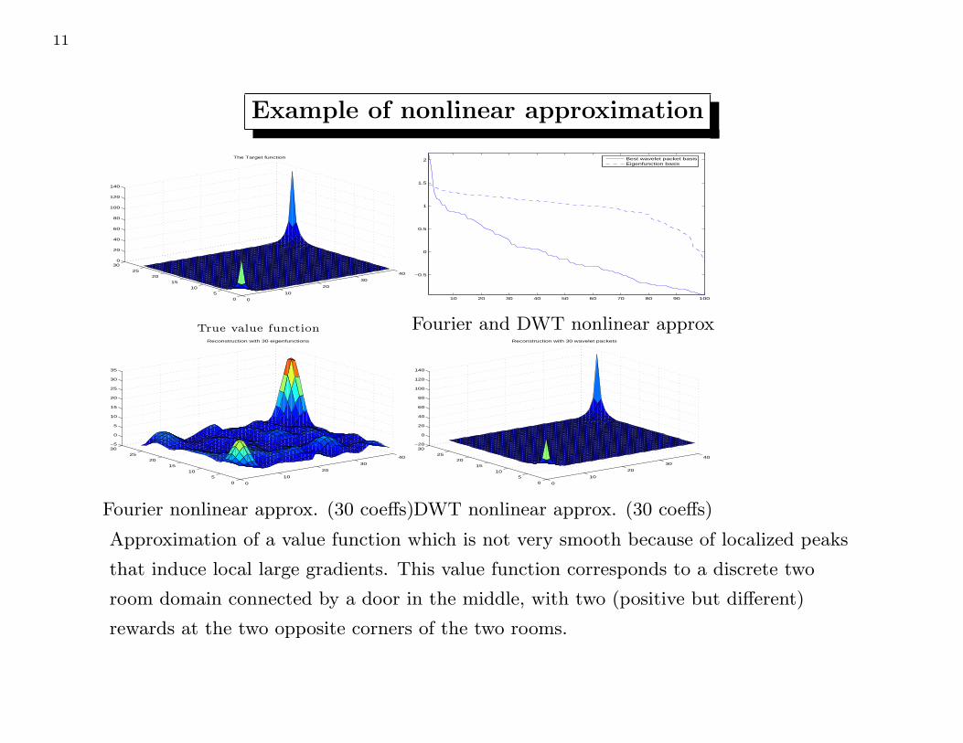
Fourier nonlinear approx. (30 coeffs)

0

10

20

30

40

0

5

10

15

20

25

30−20

0

20

40

60

80

100

120

140

Reconstruction with 30 wavelet packets

DWT nonlinear approx. (30 coeffs)

Approximation of a value function which is not very smooth because of localized peaks

that induce local large gradients. This value function corresponds to a discrete two

room domain connected by a door in the middle, with two (positive but different)

rewards at the two opposite corners of the two rooms.

12

Example of Wavelet Transform

200 400 600 800 10000

0.5

1

1.5

a1

0

0.5

1

1.5

a2

0.5

1

1.5

a3

0.5

1

1.5

a4

0.5

1

1.5

a5

0.5

1

1.5

a6

0.60.8

11.21.4

a7

0

0.5

1

a8

0

1

2

s

Signal and Approximation(s)

0

1

2

s

cfs

Coefs, Signal and Detail(s)

87654321

−0.5

0

0.5

d8

−0.1

0

0.1d

7

−0.1

0

0.1

d6

−0.1

0

0.1

d5

−0.1−0.05

00.05

d4

−0.05

0

0.05

d3

−0.05

0

0.05

d2

200 400 600 800 1000−0.04−0.02

00.020.040.06

d1

Wavelet transform. First column, top to bottom: projections onto scaling subspaces Vj (Daubechies-8) at increasing

resolution. Top of second column: wavelet transform of the original signal: horizontal axis corresponds to location,

vertical axis to scales (finer scales at the bottom). Second plot: reconstructed signal. Other plots in second column:

wavelet coefficients at increasing resolution. With 4.65% of the coefficients it is possible to recover 99.98% of the

energy (L2-norm) of the signal.

13

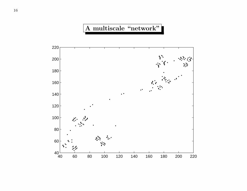
Multiscale geometry and Markov processes

In many situations the graph/manifold representing the state space contains

clusters at different scales, separated by bottlenecks. A Markov process (e.g.

associated with a policy) on such a space will be “nearly decomposable” (or

lumpable), at different time-scales. For example in the two-room problem, at a

certain large time scale, may be approximated by a two-state problem. In

general there may be more bottlenecks and decompositions, depending on the

time-scale at which the problem is considered.

This generalizes Euclidean constructions of wavelets, much used in mathematical

analysis and signal processing, and extends it not only to the analysis of

functions, but also to the analysis of Markov processes.

14

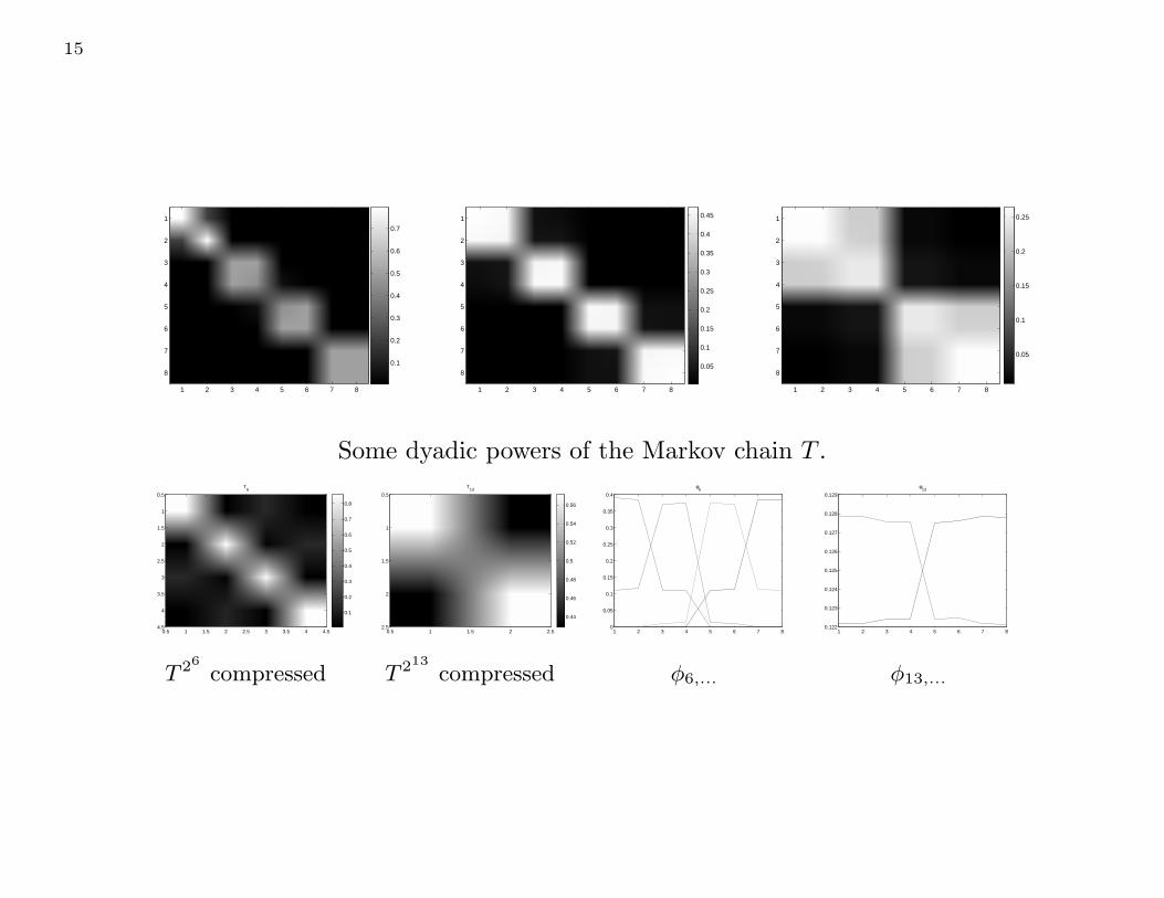
Abstraction of Markov chains

We now consider a simple example of a Markov chain on a graph with 8 states.

T =

0.80 0.20 0.00 0.00 0.00 0.00 0.00 0.00

0.20 0.79 0.01 0.00 0.00 0.00 0.00 0.00

0.00 0.01 0.49 0.50 0.00 0.00 0.00 0.00

0.00 0.00 0.50 0.499 0.001 0.00 0.00 0.00

0.00 0.00 0.00 0.001 0.499 0.50 0.00 0.00

0.00 0.00 0.00 0.00 0.50 0.49 0.01 0.00

0.00 0.00 0.00 0.00 0.00 0.01 0.49 0.50

0.00 0.00 0.00 0.00 0.00 0.00 0.50 0.50

From the matrix it is clear that the states are grouped into four pairs {ν1, ν2},

{ν3, ν4}, {ν5, ν6}, and {ν7, ν8}, with weak interactions between the the pairs.

15

1 2 3 4 5 6 7 8

1

2

3

4

5

6

7

8

0.1

0.2

0.3

0.4

0.5

0.6

0.7

1 2 3 4 5 6 7 8

1

2

3

4

5

6

7

80.05

0.1

0.15

0.2

0.25

0.3

0.35

0.4

0.45

1 2 3 4 5 6 7 8

1

2

3

4

5

6

7

8

0.05

0.1

0.15

0.2

0.25

Some dyadic powers of the Markov chain T .T

6

0.5 1 1.5 2 2.5 3 3.5 4 4.5

0.5

1

1.5

2

2.5

3

3.5

4

4.5

0.1

0.2

0.3

0.4

0.5

0.6

0.7

0.8

T 26

compressed

T13

0.5 1 1.5 2 2.5

0.5

1

1.5

2

2.5

0.44

0.46

0.48

0.5

0.52

0.54

0.56

T 213

compressed

1 2 3 4 5 6 7 80

0.05

0.1

0.15

0.2

0.25

0.3

0.35

0.4

φ6

φ6,...

1 2 3 4 5 6 7 80.122

0.123

0.124

0.125

0.126

0.127

0.128

0.129

φ13

φ13,...

16

A multiscale “network”

40 60 80 100 120 140 160 180 200 22040

60

80

100

120

140

160

180

200

220

17

0 200 4000

50

100

150

200

250

φ2,1

0 200 4000

50

100

150

200

250

φ2,2

0 200 4000

50

100

150

200

250

φ2,3

0 200 4000

50

100

150

200

250

φ2,4

0 200 4000

50

100

150

200

250

φ2,5

0 200 4000

50

100

150

200

250

φ2,6

0 200 4000

50

100

150

200

250

φ2,7

0 200 4000

50

100

150

200

250

φ2,8

0 200 4000

50

100

150

200

250

φ2,9

0 200 4000

50

100

150

200

250

φ2,10

0 200 4000

50

100

150

200

250

φ2,11

0 200 4000

50

100

150

200

250

φ2,12

0 200 4000

50

100

150

200

250

φ2,13

0 200 4000

50

100

150

200

250

φ2,14

0 200 4000

50

100

150

200

250

φ2,15

0 200 4000

50

100

150

200

250

φ2,16

0 200 4000

50

100

150

200

250

φ2,17

0 200 4000

50

100

150

200

250

φ2,18

0 200 4000

50

100

150

200

250

φ2,19

0 200 4000

50

100

150

200

250

φ2,20

0 200 4000

50

100

150

200

250

φ2,21

0 200 4000

50

100

150

200

250

φ2,22

18

0 200 4000

50

100

150

200

250

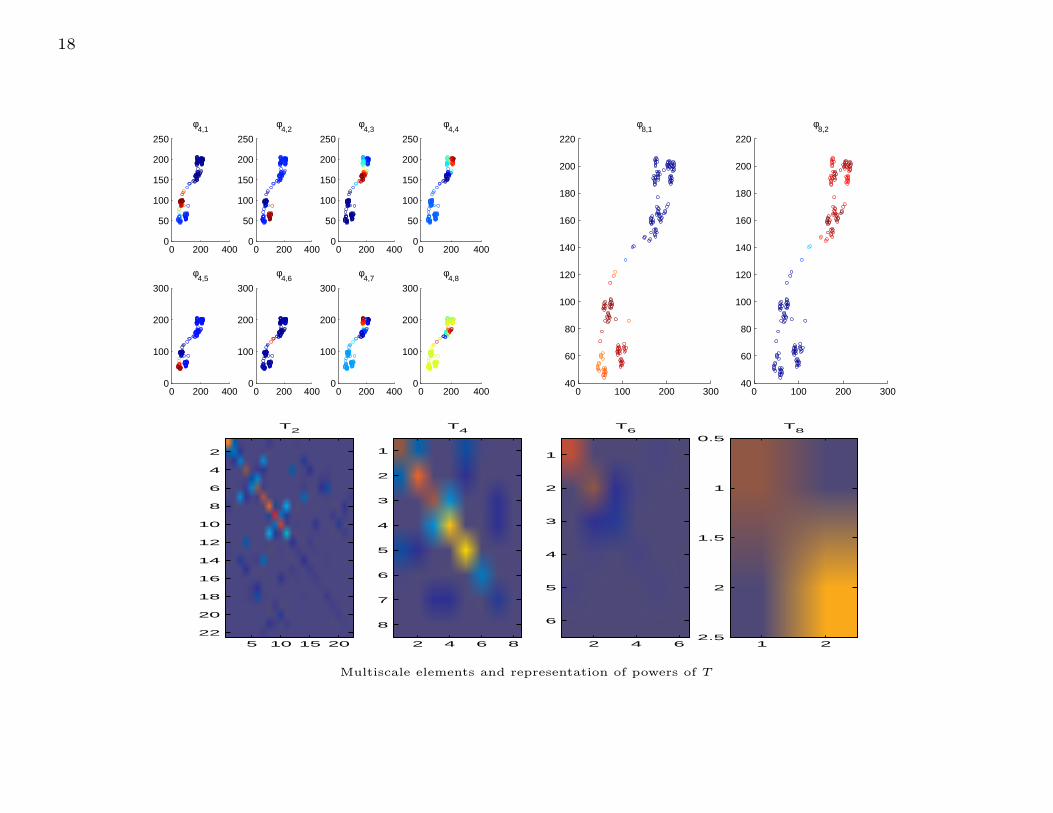
φ4,1

0 200 4000

50

100

150

200

250

φ4,2

0 200 4000

50

100

150

200

250

φ4,3

0 200 4000

50

100

150

200

250

φ4,4

0 200 4000

100

200

300

φ4,5

0 200 4000

100

200

300

φ4,6

0 200 4000

100

200

300

φ4,7

0 200 4000

100

200

300

φ4,8

0 100 200 30040

60

80

100

120

140

160

180

200

220

φ8,1

0 100 200 30040

60

80

100

120

140

160

180

200

220

φ8,2

T2

5 10 15 20

2

4

6

8

10

12

14

16

18

20

22

T4

2 4 6 8

1

2

3

4

5

6

7

8

T6

2 4 6

1

2

3

4

5

6

T8

1 2

0.5

1

1.5

2

2.5

Multiscale elements and representation of powers of T

19

Multiscale Analysis, I

We construct multiscale bases on manifolds, graphs, point clouds.

Classical constructions of wavelets are based on geometric transformations (such

as dilations, translations) of the space, transformed into actions (e.g. via

representations) on functions. There are plenty of such transformations on Rn,

certain classes of Lie groups and homogeneous spaces (with automorphisms that

resemble “anisotropic dilations”), and manifolds with large groups of

transformations.

Here the space is in general highly non-symmetric, not invariant under ”natural”

geometric transformation, and moreover it is “noisy”.

Idea: use diffusion and the heat kernel as dilations, acting on functions on the

space, to generate multiple scales.

This is connected with the work on diffusion or Markov semigroups, and

Littlewood-Paley theory of such semigroups (a la Stein).

We would like to have constructive methods for efficiently computing the

multiscale decompositions and the wavelet bases.

20

Multiscale Analysis, II

Suppose for simplicity we have a weighted graph (G, E, W ), with corresponding

Laplacian L and random walk P . Let us renormalize, if necessary, P so it has

norm 1 as an operator on L2: let T be this operator. Assume for simplicity that

T is self-adjoint, and high powers of T are low-rank: T is a diffusion, so range of

T t is spanned by smooth functions of increasingly (in t) smaller gradient.

A “typical” spectrum for the powers of T would look like this:

0 5 10 15 20 25 30

0.1

0.2

0.3

0.4

0.5

0.6

0.7

0.8

0.9

1

σ(T)

ε

V1 V

2 V

3 V

4 ...

σ(T3)

σ(T7)

σ(T15)

21

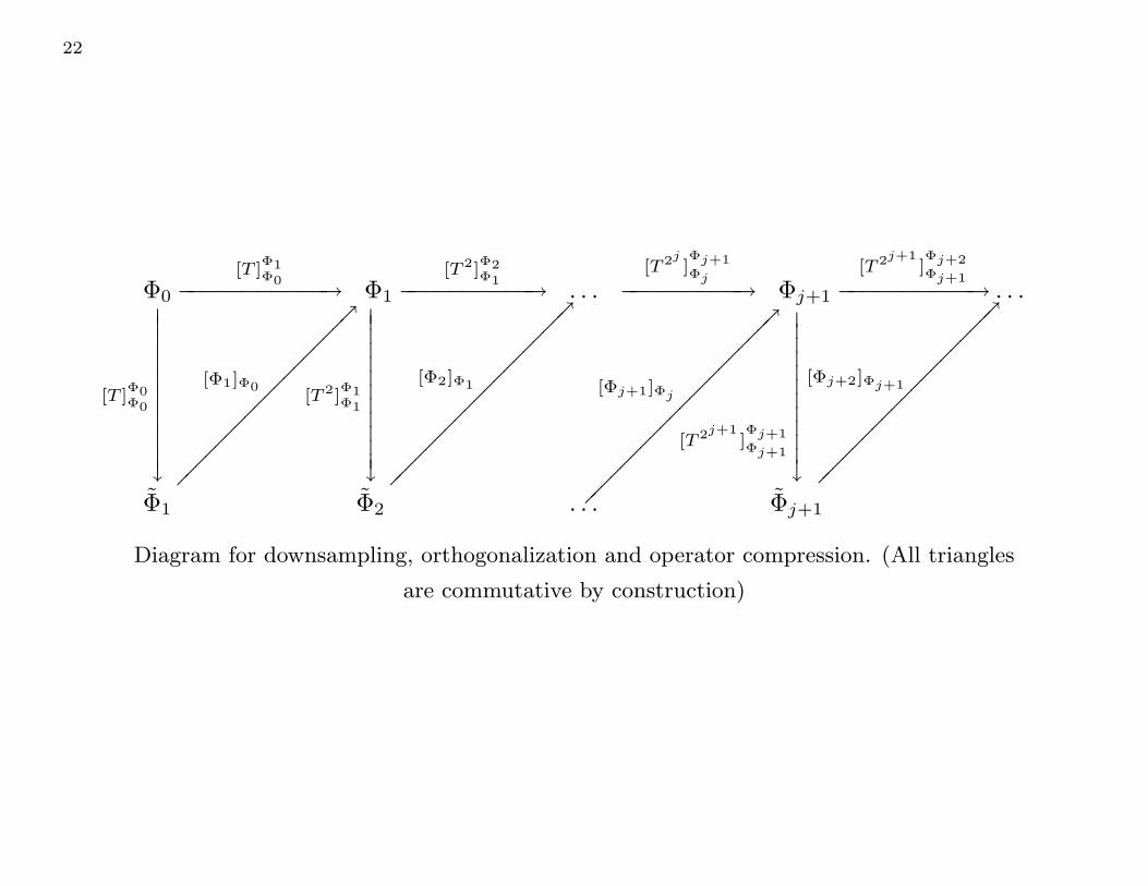
Construction of Diffusion Wavelets

22

−−−−−−−−−−−→[T ]

Φ1Φ0

−−−−−−−−−−→[T 2]

Φ2Φ1

−−−−−−−−−→[T 2j

]Φj+1Φj

−−−−−−−−−−→[T 2j+1

]Φj+2Φj+1

−−−−−−−−−−−−→

[T ]Φ0Φ0

−−−−−−−−−−−−−−−−−→

[Φ1]Φ0

−−−−−−−−−−−−→

[T 2]Φ1Φ1

−−−−−−−−−−−−−−−−−−→

[Φ2]Φ1

−−−−−−−−−−−−−−−−−−−→

[Φj+1]Φj

−−−−−−−−−−−→[T 2j+1

]Φj+1Φj+1

−−−−−−−−−−−−−−−−−−→

[Φj+2]Φj+1

Φ0 Φ1 . . . Φj+1 . . .

Φ1 Φ2 . . . Φj+1

Diagram for downsampling, orthogonalization and operator compression. (All triangles

are commutative by construction)

23

{Φj}Jj=0, {Ψj}

J−1j=0 , {[T 2j

]Φj

Φj}J

j=1 ← DiffusionWaveletTree ([T ]Φ0Φ0

, Φ0, J, SpQR, ǫ)

// [T ]Φ0Φ0

: a diffusion operator, written on the o.n. basis Φ0

// Φ0 : an orthonormal basis which ǫ-spans V0

// J : number of levels to compute

// SpQR : a function compute a sparse QR decomposition, template below.

// ǫ: precision

// Output: The orthonormal bases of scaling functions, Φj , wavelets, Ψj , and

// compressed representation of T 2j

on Φj , for j in the requested range.

for j = 0 to J − 1 do

[Φj+1]Φj, [T ]Φ1

Φ0←SpQR([T 2j

]Φj

Φj, ǫ)

Tj+1 := [T 2j+1

]Φj+1

Φj+1← [Φj+1]Φj

[T 2j

]Φj

Φj[Φj+1]

∗Φj

[Ψj ]Φj← SpQR(I〈Φj〉 − [Φj+1]Φj [Φj+1]

∗Φj

, ǫ)

end

Q, R ← SpQR (A, ǫ) // A: sparse n × n matrix, ǫ: precision

// Output: Q, R matrices, hopefully sparse, such that A =ǫ QR, Q is n × m and orthogonal,

// R is m × n, and upper triangular up to a permutation,

// the columns of Q ǫ-span the space spanned by the columns of A.

24

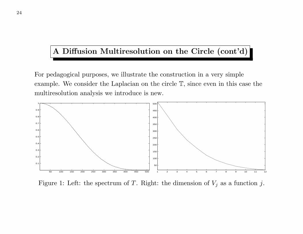
A Diffusion Multiresolution on the Circle (cont’d)

For pedagogical purposes, we illustrate the construction in a very simple

example. We consider the Laplacian on the circle T, since even in this case the

multiresolution analysis we introduce is new.

50 100 150 200 250 300 350 400 450 500

0.1

0.2

0.3

0.4

0.5

0.6

0.7

0.8

0.9

1

1 2 3 4 5 6 7 8 9 10 11 12

50

100

150

200

250

300

350

400

450

500

Figure 1: Left: the spectrum of T . Right: the dimension of Vj as a function j.

25

50 100 150 200 250 300 350 400 450 500

−0.4

−0.2

0

0.2

0.4

0.6

50 100 150 200 250 300 350 400 450 500

−0.4

−0.3

−0.2

−0.1

0

0.1

0.2

0.3

0.4

0.5

50 100 150 200 250 300 350 400 450 500

−0.2

−0.15

−0.1

−0.05

0

0.05

0.1

0.15

0.2

0.25

0.3

50 100 150 200 250 300 350 400 450 500−0.08

−0.06

−0.04

−0.02

0

0.02

0.04

0.06

0.08

0.1

Figure 2: Some scaling functions in V1 (top left), in V3 (top right), V6 (bottom

left) and V12 (bottom right).

26

50 100 150 200 250 300 350 400 450

50

100

150

200

250

300

350

400

450

500

−5.5

−5

−4.5

−4

−3.5

−3

−2.5

−2

−1.5

−1

−0.5

50 100 150 200 250 300 350 400

50

100

150

200

250

300

350

400

450 −5.5

−5

−4.5

−4

−3.5

−3

−2.5

−2

−1.5

−1

−0.5

20 40 60 80 100 120 140 160

20

40

60

80

100

120

140

160

180

200

220 −5.5

−5

−4.5

−4

−3.5

−3

−2.5

−2

−1.5

−1

−0.5

2 4 6 8 10 12 14 16 18 20

5

10

15

20

25

30−5.5

−5

−4.5

−4

−3.5

−3

−2.5

−2

−1.5

−1

−0.5

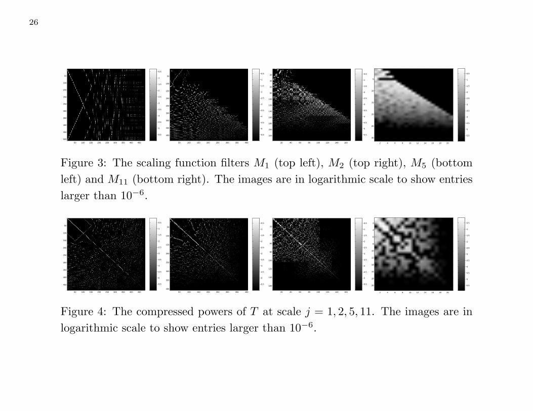
Figure 3: The scaling function filters M1 (top left), M2 (top right), M5 (bottom

left) and M11 (bottom right). The images are in logarithmic scale to show entries

larger than 10−6.

50 100 150 200 250 300 350 400 450

50

100

150

200

250

300

350

400

450 −5.5

−5

−4.5

−4

−3.5

−3

−2.5

−2

−1.5

−1

−0.5

50 100 150 200 250 300 350 400

50

100

150

200

250

300

350

400

−5.5

−5

−4.5

−4

−3.5

−3

−2.5

−2

−1.5

−1

−0.5

20 40 60 80 100 120 140 160

20

40

60

80

100

120

140

160−5.5

−5

−4.5

−4

−3.5

−3

−2.5

−2

−1.5

−1

−0.5

2 4 6 8 10 12 14 16 18 20

2

4

6

8

10

12

14

16

18

20 −5.5

−5

−4.5

−4

−3.5

−3

−2.5

−2

−1.5

−1

−0.5

Figure 4: The compressed powers of T at scale j = 1, 2, 5, 11. The images are in

logarithmic scale to show entries larger than 10−6.

29

Thinking multiscale on graphs...

Investigating other constructions:

• Biorthogonal diffusion wavelets, in which scaling functions are probability

densities (useful for multiscale Markov chains)

• Top-bottom constructions: recursive subdivision

• Both...

Applications besides Markov Decision Processes:

• Document organization and classification

• Nonlinear Analysis of Images

• Semi-supervised learning through diffusion processes on data


Outline




-2 -1.5 -1 -0.5 0 0.5 1 1.5 2-8

-6

-4

-2

0

2

4

6

8 Fourier


Wavelets

Inverted pendulum

5 10 15 20 25

5

10

15

20

25

-16

-14

-12

-10

-8

-6

-4

-2

0

2





BuildGraph


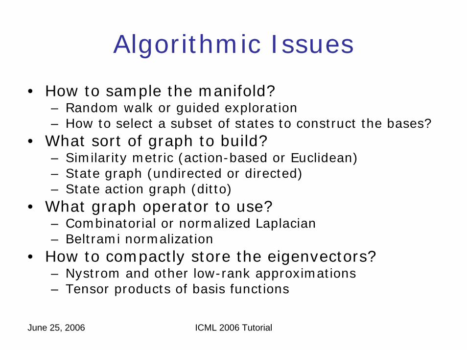
Algorithmic Issues

• How to sample the manifold?– Random walk or guided exploration– How to select a subset of states to construct the bases?

• What sort of graph to build?– Similarity metric (action-based or Euclidean)– State graph (undirected or directed)– State action graph (ditto)

• What graph operator to use?– Combinatorial or normalized Laplacian– Beltrami normalization

• How to compactly store the eigenvectors?– Nystrom and other low-rank approximations– Tensor products of basis functions


Random Sampling from a Continuous Manifold

−1.2 −1 −0.8 −0.6 −0.4 −0.2 0 0.2 0.4 0.6−0.1

−0.05

0

0.05

0.1

−1.2 −1 −0.8 −0.6 −0.4 −0.2 0 0.2 0.4 0.6−0.1

−0.05

0

0.05

0.1

Mountaincar domain


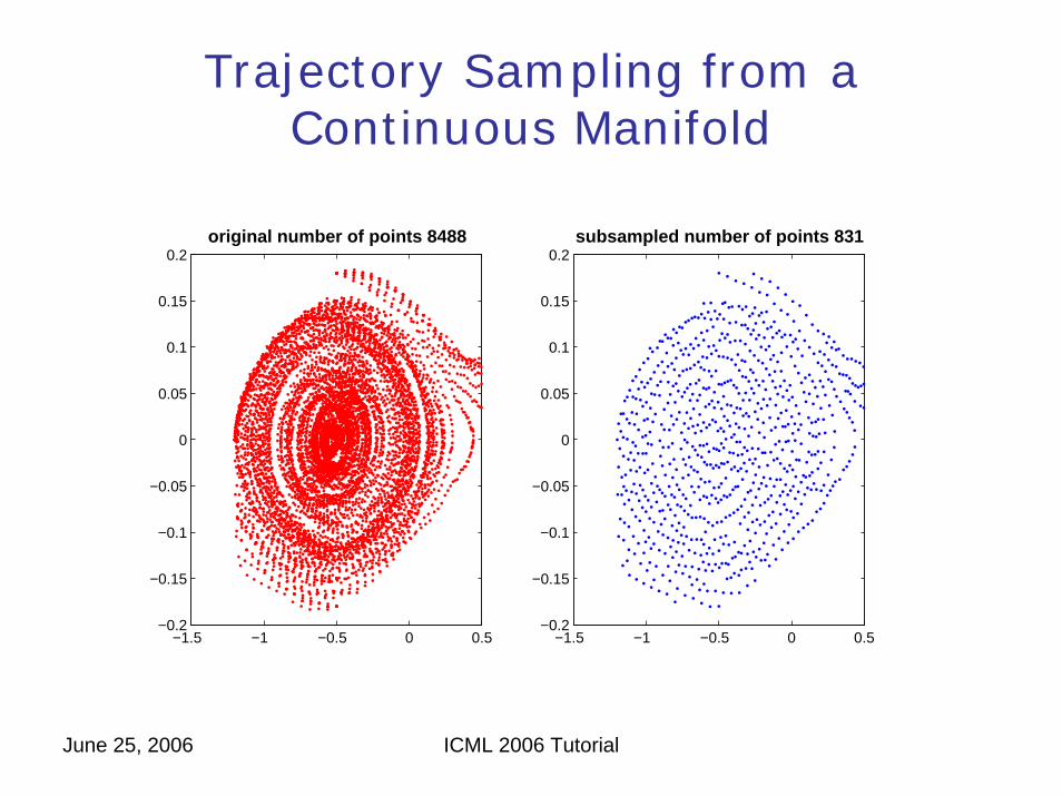
Trajectory Sampling from a Continuous Manifold

−1.5 −1 −0.5 0 0.5−0.2

−0.15

−0.1

−0.05

0

0.05

0.1

0.15

0.2original number of points 8488

−1.5 −1 −0.5 0 0.5−0.2

−0.15

−0.1

−0.05

0

0.05

0.1

0.15

0.2subsampled number of points 831


Type of Graphs

• Graphs on the state space– Undirected graph (weighted or unweighted)– Directed graph (assume strongly connected)

• Graphs on state action space [Osentoski, 2006]

– Basis functions directly represent φ(s,a)– Graph grows larger

• Other types of graph– Graphs on state controller space (hierarchical RL)

– Hypergraphs (multivalued relations)


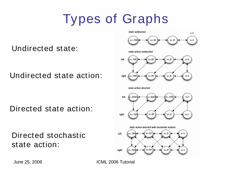
Types of Graphs

Undirected state:

Undirected state action:

Directed state action:

Directed stochasticstate action:


Similarity Metrics

• The graph is constructed using a similarity metric– In discrete spaces, connect state s to s’ if an

action led the agent from s → s’– Action respecting embedding [Bowling, ICML 2005]

• Local distance metrics:– Nearest neighbor: connect an edge from s to s’

if s’ is one of k nearest neighbors of s– Heat kernel: connect s to s’ if | s –s’|2 < ε with

weight w(s,s’)= e-| s – s’|2/2 < ε


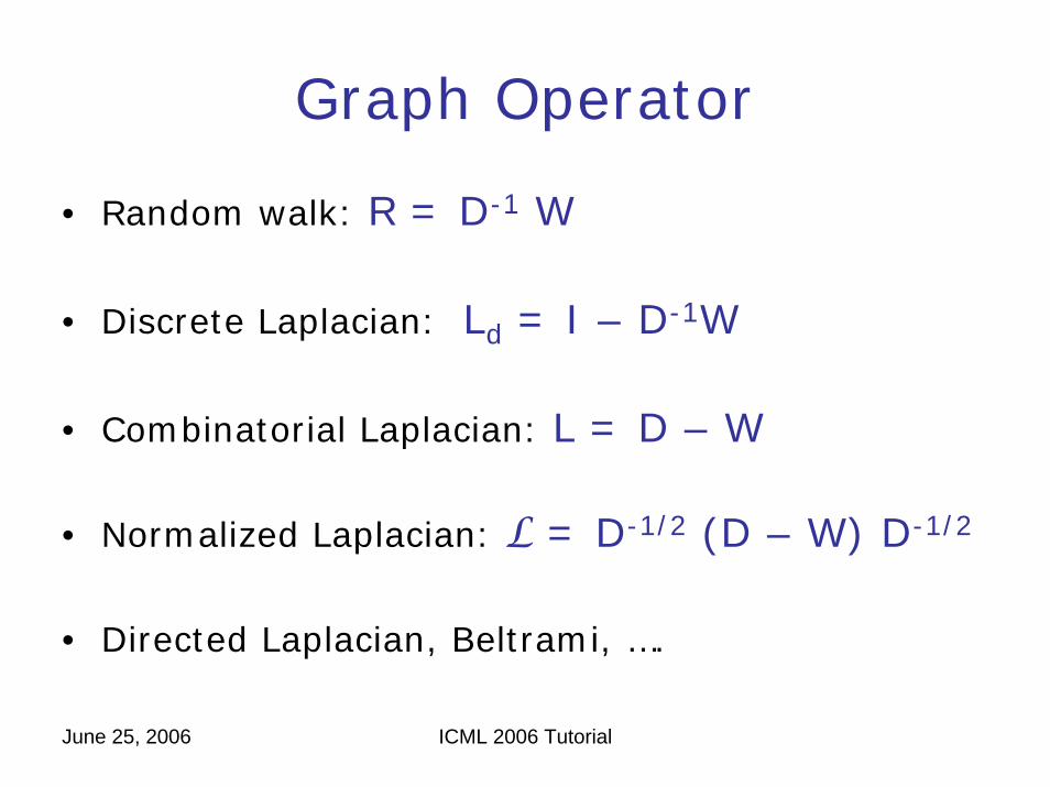
Graph Operator

• Random walk: R = D-1 W

• Discrete Laplacian: Ld = I – D-1W

• Combinatorial Laplacian: L = D – W

• Normalized Laplacian: L = D-1/2 (D – W) D-1/2

• Directed Laplacian, Beltrami, ….


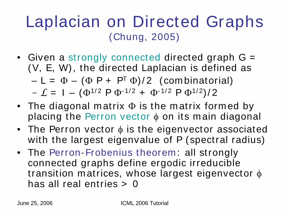
Laplacian on Directed Graphs(Chung, 2005)

• Given a strongly connected directed graph G = (V, E, W), the directed Laplacian is defined as– L = Φ – (Φ P + PT Φ)/2 (combinatorial)– L = I – (Φ1/2 P Φ-1/2 + Φ-1/2 P Φ1/2)/2

• The diagonal matrix Φ is the matrix formed by placing the Perron vector φ on its main diagonal

• The Perron vector φ is the eigenvector associated with the largest eigenvalue of P (spectral radius)

• The Perron-Frobenius theorem: all strongly connected graphs define ergodic irreducible transition matrices, whose largest eigenvector φhas all real entries > 0


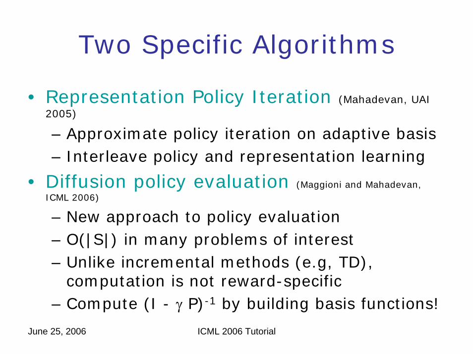
Two Specific Algorithms

• Representation Policy Iteration (Mahadevan, UAI 2005)

– Approximate policy iteration on adaptive basis– Interleave policy and representation learning

• Diffusion policy evaluation (Maggioni and Mahadevan, ICML 2006)

– New approach to policy evaluation– O(|S|) in many problems of interest– Unlike incremental methods (e.g, TD),

computation is not reward-specific– Compute (I - γ P)-1 by building basis functions!


Representation Policy Iteration(Mahadevan, UAI 2005)

TrajectoriesRepresentation

Learner

“Greedy”Policy

Policyimprovement

Policyevaluation

“Actor”

“Critic” Laplacian/wavelet bases


Least-Squares Policy Iteration(Lagoudakis and Parr, JMLR 2003)

Random walk generates transitions D = (st, at, r, st’),…

Solve the equation:


Scaling Fourier and Wavelet Bases

• Factored MDPs generate product (tensor) spaces– It is possible to represent spectral bases

compactly for large factored MDPs– Basis functions can be represented in space

independent of the size of the state space – Fourier analysis on groups: compact

representations• Continuous spaces can be handled by sampling

the underlying manifold and constructing a graph– Nystrom interpolation method for extension of

eigenfunctions– Low-rank approximations of diffusion matrices


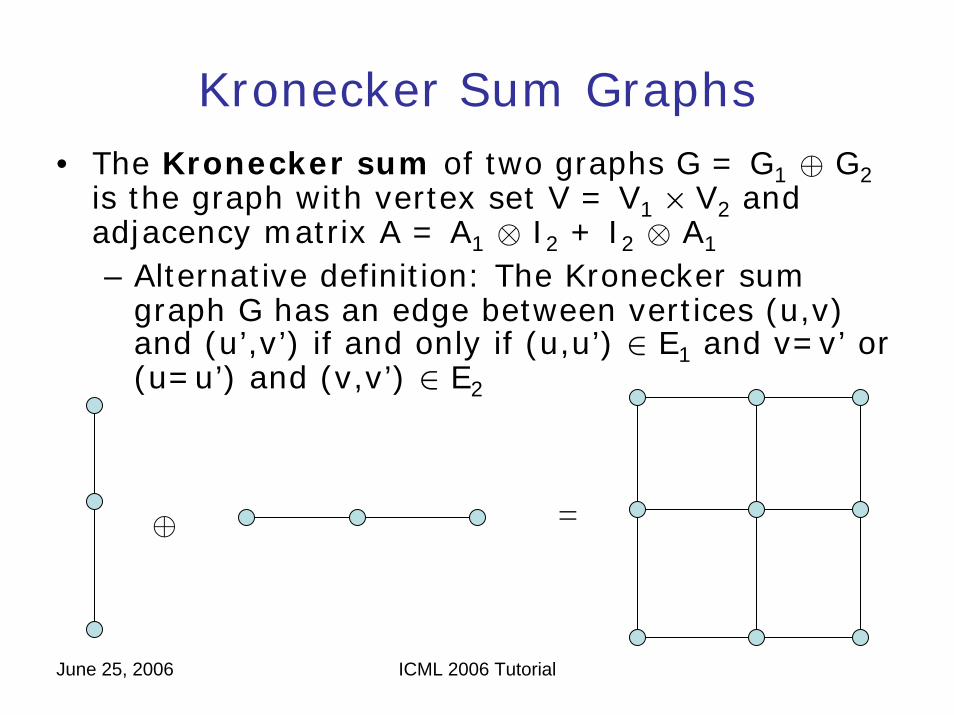
Kronecker Sum Graphs• The Kronecker sum of two graphs G = G1 ⊕ G2

is the graph with vertex set V = V1 × V2 and adjacency matrix A = A1 ⊗ I2 + I2 ⊗ A1

– Alternative definition: The Kronecker sum graph G has an edge between vertices (u,v) and (u’,v’) if and only if (u,u’) ∈ E1 and v=v’ or (u=u’) and (v,v’) ∈ E2

⊕ =


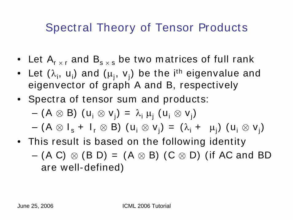
Spectral Theory of Tensor Products

• Let Ar × r and Bs × s be two matrices of full rank• Let (λi, ui) and (μj, vj) be the ith eigenvalue and

eigenvector of graph A and B, respectively• Spectra of tensor sum and products:

– (A ⊗ B) (ui ⊗ vj) = λi μj (ui ⊗ vj)– (A ⊗ Is + Ir ⊗ B) (ui ⊗ vj) = (λi + μj) (ui ⊗ vj)

• This result is based on the following identity – (A C) ⊗ (B D) = (A ⊗ B) (C ⊗ D) (if AC and BD

are well-defined)


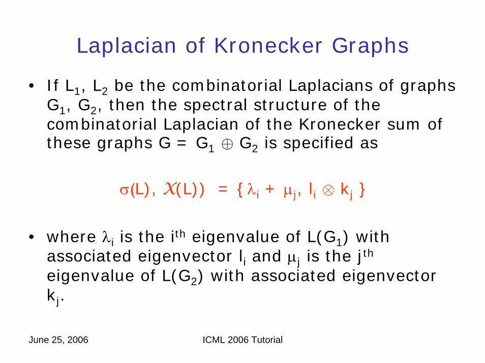
Laplacian of Kronecker Graphs

• If L1, L2 be the combinatorial Laplacians of graphs G1, G2, then the spectral structure of the combinatorial Laplacian of the Kronecker sum of these graphs G = G1 ⊕ G2 is specified as

σ(L), X(L)) = {λi + μj, li ⊗ kj }

• where λi is the ith eigenvalue of L(G1) with associated eigenvector li and μj is the jtheigenvalue of L(G2) with associated eigenvector kj.


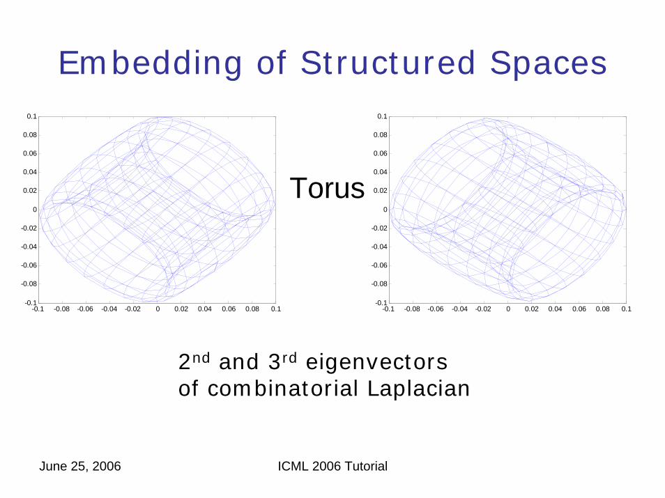
Embedding of Structured Spaces

-0.1 -0.08 -0.06 -0.04 -0.02 0 0.02 0.04 0.06 0.08 0.1-0.1

-0.08

-0.06

-0.04

-0.02

0

0.02

0.04

0.06

0.08

0.1

Torus

2nd and 3rd eigenvectorsof combinatorial Laplacian

-0.1 -0.08 -0.06 -0.04 -0.02 0 0.02 0.04 0.06 0.08 0.1-0.1

-0.08

-0.06

-0.04

-0.02

0

0.02

0.04

0.06

0.08

0.1


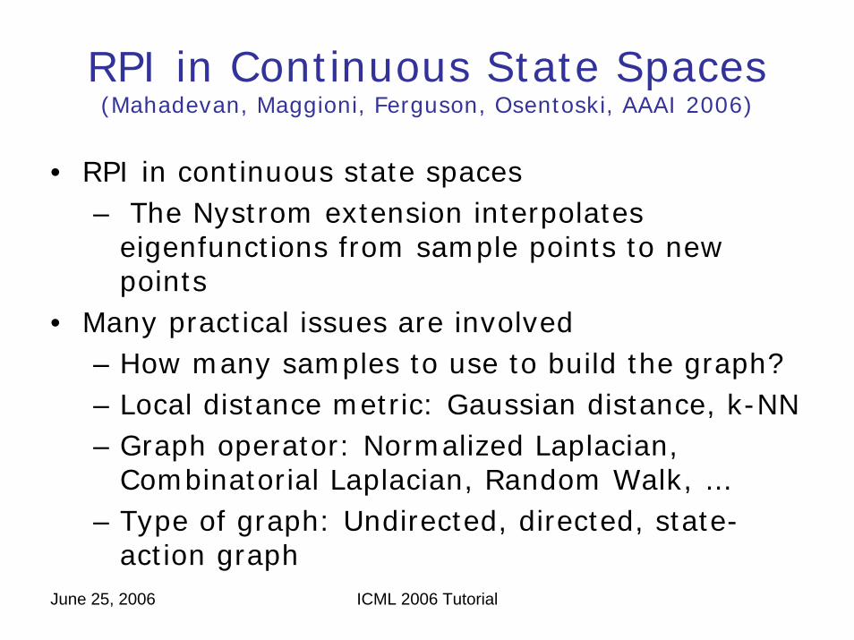
RPI in Continuous State Spaces(Mahadevan, Maggioni, Ferguson, Osentoski, AAAI 2006)

• RPI in continuous state spaces– The Nystrom extension interpolates

eigenfunctions from sample points to new points

• Many practical issues are involved– How many samples to use to build the graph?– Local distance metric: Gaussian distance, k-NN– Graph operator: Normalized Laplacian,

Combinatorial Laplacian, Random Walk, …– Type of graph: Undirected, directed, state-

action graph


The Nystrom method(Williams and Seeger, NIPS 2001)

• The Nystrom approximation was developed in the context of solving integral equations

∫D K(t,s) Φ(s) ds = λ Φ(t), t ∈ D

• A quadrature approximation of the integral: ∫D K(t,s) Φ(s) ds = ∑j wj k(x,s) φ(sj)

leads to the following equation∑j wj k(x,s) φ(sj) = λ φ(x)

• which rewritten gives the Nystrom extensionφm(x) = 1/λm ∑j wj k(x,s) φm(sj)


Outline




Experimental Testbeds

• Discrete MDPs:– One dimensional chains [Koller and Parr, UAI 2001]

– Two dimensional “room” environments [Mannor, McGovern, Simsek et al]

– Factored MDPs (Sallans and Hinton, JMLR 2003)

• Continuous MDPs:– Inverted pendulum and mountain car


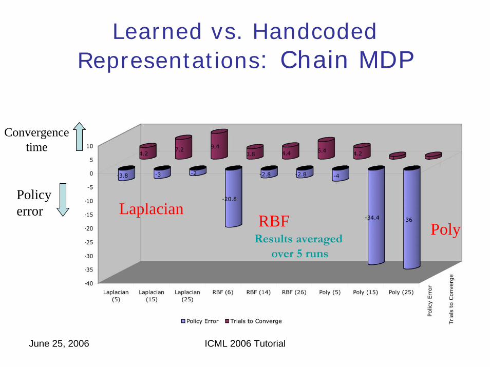
Learned vs. HandcodedRepresentations: Chain MDP

Convergencetime

Policyerror Laplacian

RBF PolyResults averaged

over 5 runs


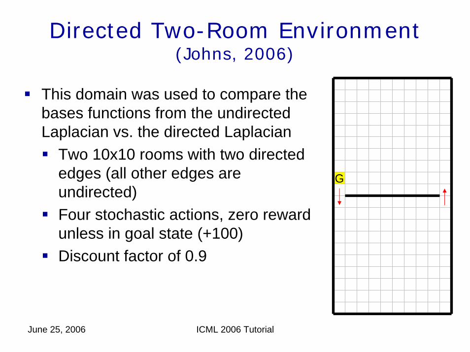
Directed Two-Room Environment(Johns, 2006)

This domain was used to compare the bases functions from the undirected Laplacian vs. the directed Laplacian

Two 10x10 rooms with two directed edges (all other edges are undirected)Four stochastic actions, zero reward unless in goal state (+100)Discount factor of 0.9

G


Directed vs. Undirected Laplacian

• The first eigenvector of the normalized Laplacian shows the difference directionality makes on the steady-state distribution

Directed Undirected


Results: Directed vs. Unidrected Laplacian(Johns, 2006)

• The undirected Laplacian results in a poorer approximation because it ignores directionality

Exact VF Undirected Dir. Combinatorial


Comparison of Undirected vs. Directed Laplacians


Blockers Domain(Sallans and Hinton, JMLR 2003)

1 2 3 4 5 6 7 8 9 10

1

2

3

4

5

6

7

8

9

10

123

1 2 3 4 5 6 7 8 9 10

1

2

3

4

5

6

7

8

9

10

1 2

3

Large state space of > 106 states


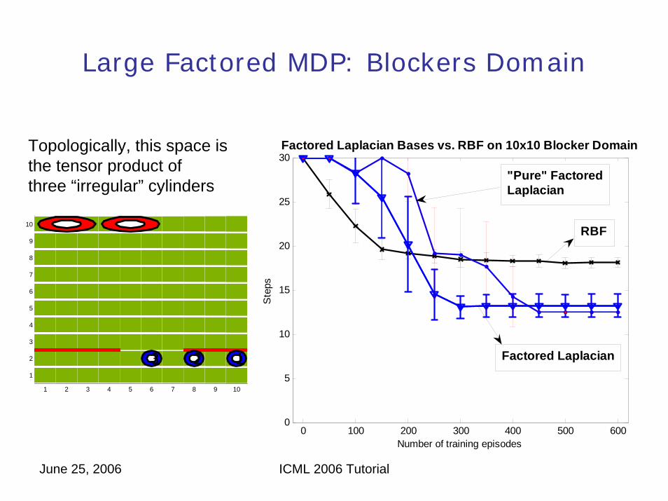
Large Factored MDP: Blockers Domain

Topologically, this space isthe tensor product ofthree “irregular” cylinders

1 2 3 4 5 6 7 8 9 10

1

2

3

4

5

6

7

8

9

10

123

0 100 200 300 400 500 6000

5

10

15

20

25

30Factored Laplacian Bases vs. RBF on 10x10 Blocker Domain

Number of training episodes

Ste

ps

RBF

Factored Laplacian

"Pure" FactoredLaplacian


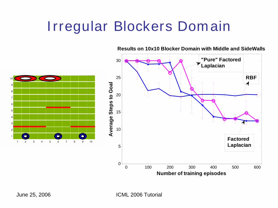
Irregular Blockers Domain

0 100 200 300 400 500 6000

5

10

15

20

25

30

Results on 10x10 Blocker Domain with Middle and SideWalls


Ave

rage

Ste

ps to

Goa

l

RBF

FactoredLaplacian

"Pure" FactoredLaplacian


RPI on Inverted Pendulum(Mahadevan, Maggioni, Ferguson, Osentoski, AAAI 2006)

-1

-0.5

0

0.5

1 -3

-2

-1

0

1

2

3

-1

-0.5

0

0.5

1

Angular Velocity

Approximate Value Function for Inverted Pendulum using Laplacian Eigenfunctions

Angle

Q-v

alue

for o

ptim

al p

olic

y

-2 -1 0 1 2-10

-5

0

5

10Original data

-2 -1 0 1 2-10

-5

0

5

10Subsampled data


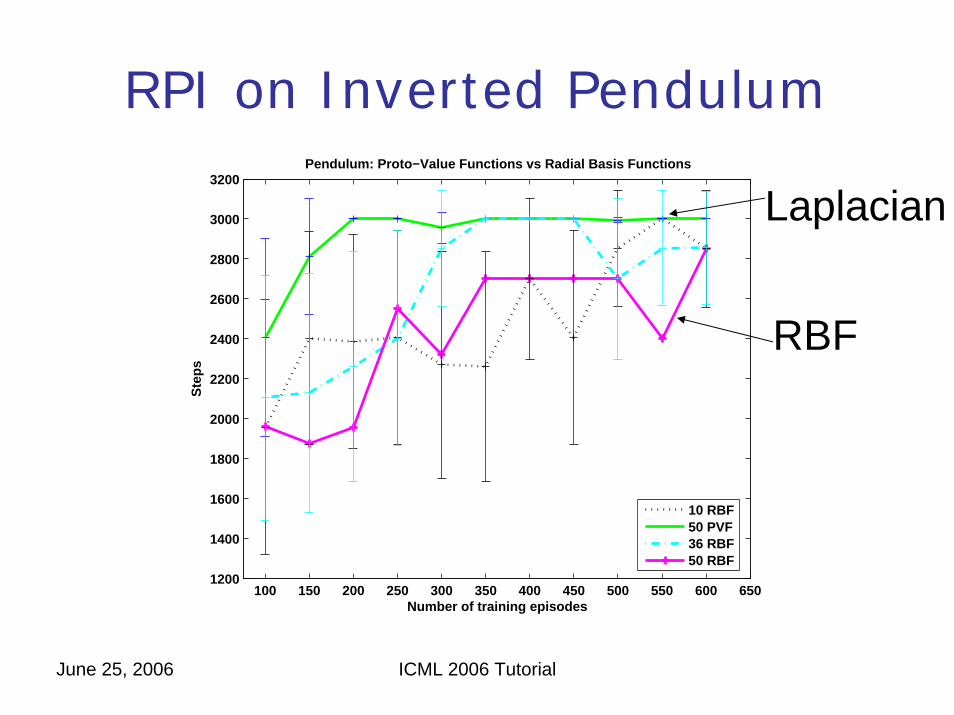
RPI on Inverted Pendulum

100 150 200 250 300 350 400 450 500 550 600 6501200

1400

1600

1800

2000

2200

2400

2600

2800

3000

3200Pendulum: Proto−Value Functions vs Radial Basis Functions


Ste

ps

10 RBF50 PVF36 RBF50 RBF

Laplacian

RBF

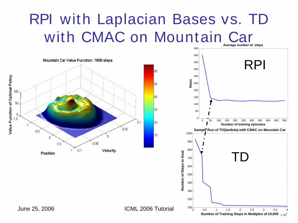
June 25, 2006 ICML 2006 Tutorial 0 0.5 1 1.5 2 2.5 3 3.5 4

x 104

100

200

300

400

500

600

700

800

900

1000

Number of Training Steps in Multiples of 10,000

Num

ber o

f Ste

ps to

Goa

l

Sample Run of TD(lambda) with CMAC on Mountain Car

RPI with Laplacian Bases vs. TD with CMAC on Mountain Car

0 50 100 150 200 250 300 350 400 450 5000

50

100

150

200

250

300

350

400

450

500Average number of steps


Step

s

RPI

TD

30

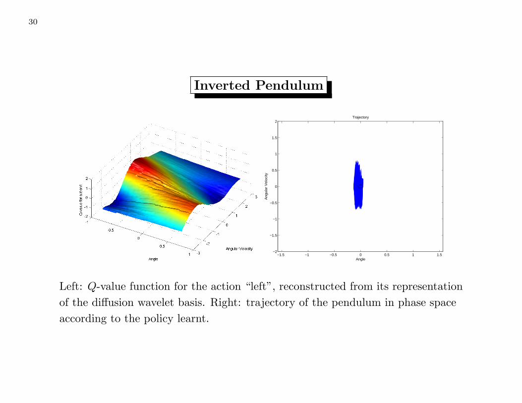
Inverted Pendulum

−1.5 −1 −0.5 0 0.5 1 1.5−2

−1.5

−1

−0.5

0

0.5

1

1.5

2Trajectory

AngleA

ngul

ar V

eloc

ity

Left: Q-value function for the action “left”, reconstructed from its representation

of the diffusion wavelet basis. Right: trajectory of the pendulum in phase space

according to the policy learnt.

31

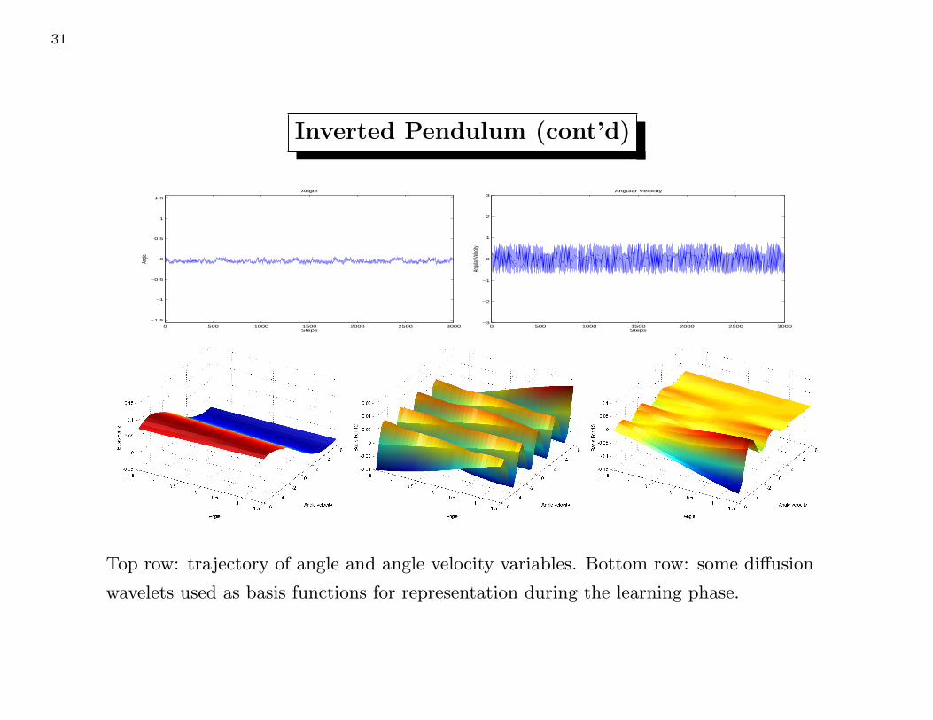
Inverted Pendulum (cont’d)

0 500 1000 1500 2000 2500 3000

−1.5

−1

−0.5

0

0.5

1

1.5

Angle

Steps

Angle

0 500 1000 1500 2000 2500 3000−3

−2

−1

0

1

2

3Angular Velocity

Steps

Angu

lar Ve

locity

Top row: trajectory of angle and angle velocity variables. Bottom row: some diffusion

wavelets used as basis functions for representation during the learning phase.

32

Inverted Pendulum (cont’d)

0 50 100 150 200 250 300 350 4000

500

1000

1500

2000

2500

3000

3500Average number of balancing steps


Ste

ps

0 50 100 150 200 250 300 350 400

0

0.1

0.2

0.3

0.4

0.5

0.6

0.7

0.8

0.9

1

Average probability of success


Pro

babi

lity

0 50 100 150 200 250 300 350 4000

500

1000

1500

2000

2500

3000Worst and best policy: average number of balancing steps


Ste

ps

Measures of performance based on 20 experiments, as a function of number of training

runs (each of which of length at most 100). From left to right: average number of

successful steps of inverted pendulum balancing, average probability of succeeding in

balancing for at least 3000 steps, and worst and best number of balancing steps. Each

simulation was stopped and considered successful after 3000 steps, which biases the first

and third graphs downwards.

33

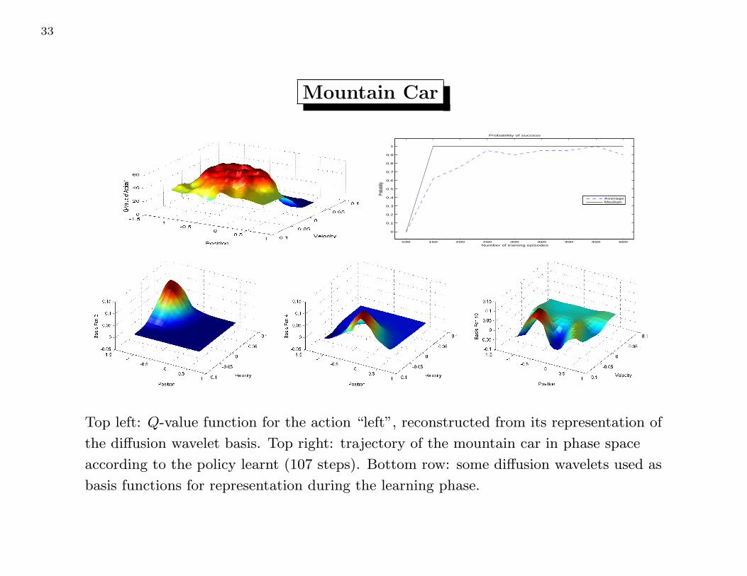
Mountain Car

100 150 200 250 300 350 400 450 500

0

0.1

0.2

0.3

0.4

0.5

0.6

0.7

0.8

0.9

1

Probability of success


Proba

bility

AverageMedian

Top left: Q-value function for the action “left”, reconstructed from its representation of

the diffusion wavelet basis. Top right: trajectory of the mountain car in phase space

according to the policy learnt (107 steps). Bottom row: some diffusion wavelets used as

basis functions for representation during the learning phase.

34

Mountain Car (cont’d)

100 150 200 250 300 350 400 450 500

0

0.1

0.2

0.3

0.4

0.5

0.6

0.7

0.8

0.9

1



Pro

babi

lity

AverageMedian

100 150 200 250 300 350 400 450 500

0

0.1

0.2

0.3

0.4

0.5

0.6

0.7

0.8

0.9

1



Pro

babi

lity

AverageMedian

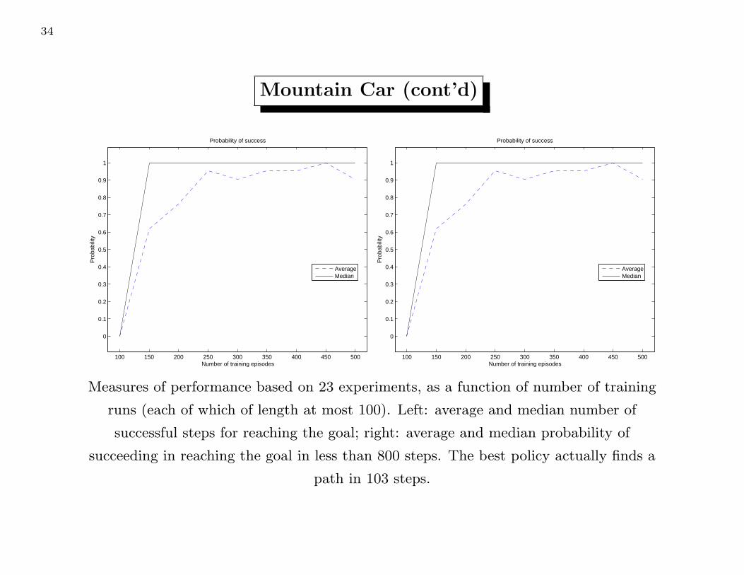
Measures of performance based on 23 experiments, as a function of number of training

runs (each of which of length at most 100). Left: average and median number of

successful steps for reaching the goal; right: average and median probability of

succeeding in reaching the goal in less than 800 steps. The best policy actually finds a

path in 103 steps.

35

Multiscale inversion

The multiscale construction enables a direct solution of Bellman’s equation. The

algorithm consists of two parts:

(i) a pre-computation step, that depends on the structure of the state space and

on the policy, and yields the multiscale analysis described above.

(ii) an inversion step which uses the multiscale structure built in the

pre-computation step to efficiently compute the solution of Bellman’s

equations for a given reward function.

36

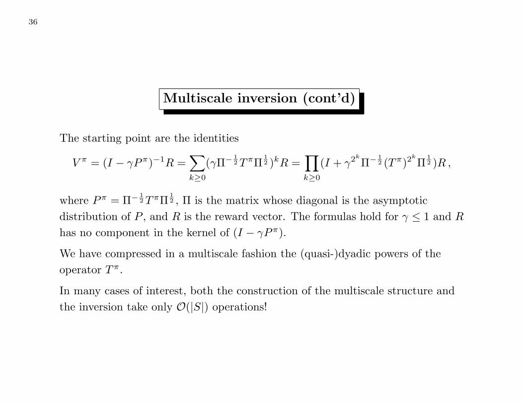
Multiscale inversion (cont’d)

The starting point are the identities

V π = (I − γPπ)−1R =∑

k≥0

(γΠ− 12 TπΠ

12 )kR =

∏

k≥0

(I + γ2k

Π− 12 (Tπ)2

k

Π12 )R ,

where Pπ = Π− 12 TπΠ

12 , Π is the matrix whose diagonal is the asymptotic

distribution of P , and R is the reward vector. The formulas hold for γ ≤ 1 and R

has no component in the kernel of (I − γPπ).

We have compressed in a multiscale fashion the (quasi-)dyadic powers of the

operator Tπ.

In many cases of interest, both the construction of the multiscale structure and

the inversion take only O(|S|) operations!

37

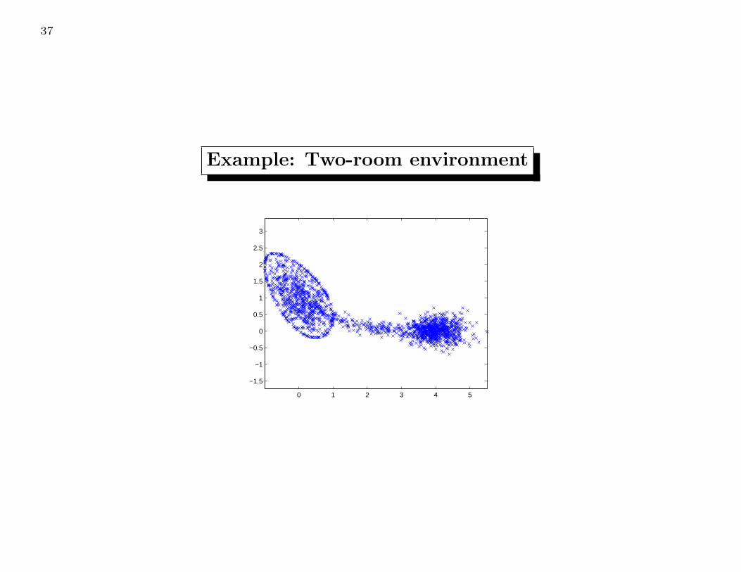
Example: Two-room environment

0 1 2 3 4 5

−1.5

−1

−0.5

0

0.5

1

1.5

2

2.5

3

38

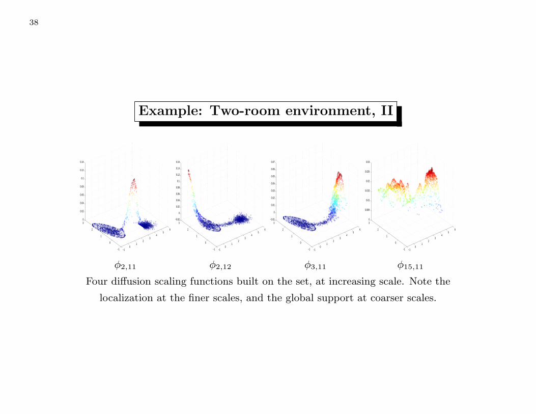
Example: Two-room environment, II

−10

12

34

56

−1

0

1

2

30

0.02

0.04

0.06

0.08

0.1

0.12

0.14

φ2,11

−10

12

34

56

−1

0

1

2

3−0.02

0

0.02

0.04

0.06

0.08

0.1

0.12

0.14

0.16

φ2,12

−10

12

34

56

−1

0

1

2

3−0.01

0

0.01

0.02

0.03

0.04

0.05

0.06

0.07

φ3,11

−10

12

34

56

−1

0

1

2

30

0.005

0.01

0.015

0.02

0.025

0.03

φ15,11

Four diffusion scaling functions built on the set, at increasing scale. Note the

localization at the finer scales, and the global support at coarser scales.

39

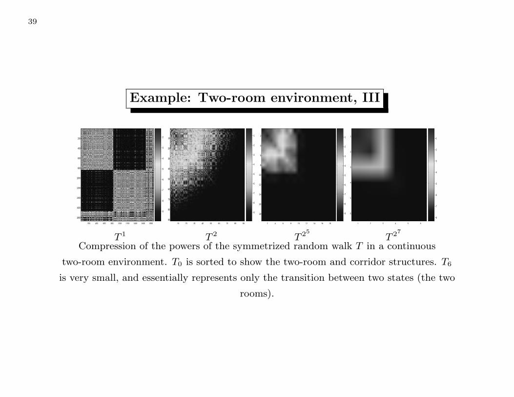
Example: Two-room environment, III

200 400 600 800 1000 1200 1400 1600 1800

200

400

600

800

1000

1200

1400

1600

1800

−9

−8

−7

−6

−5

−4

−3

−2

T 1

10 20 30 40 50 60 70 80 90

10

20

30

40

50

60

70

80

90

−9

−8

−7

−6

−5

−4

−3

−2

−1

T 2

2 4 6 8 10 12 14 16 18

2

4

6

8

10

12

14

16

18 −9

−8

−7

−6

−5

−4

−3

−2

−1

T 25

1 2 3 4 5 6

1

2

3

4

5

6

−8

−7

−6

−5

−4

−3

−2

−1

T 27

Compression of the powers of the symmetrized random walk T in a continuous

two-room environment. T0 is sorted to show the two-room and corridor structures. T6

is very small, and essentially represents only the transition between two states (the two

rooms).

40

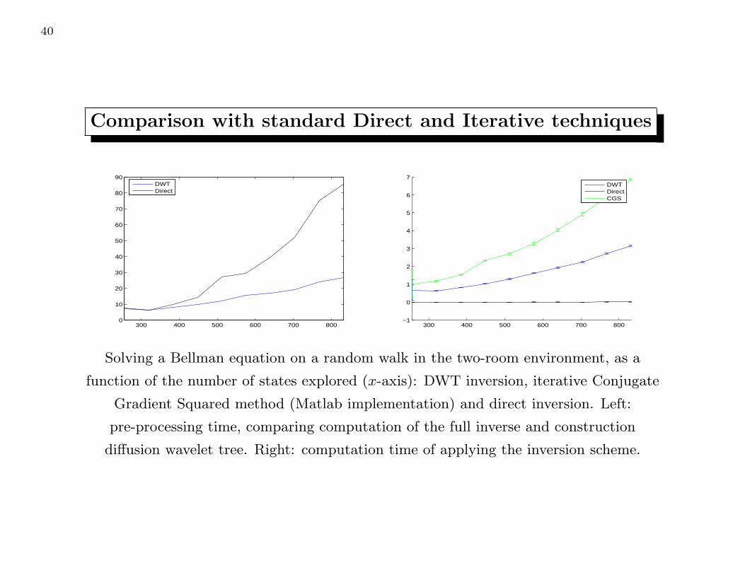
Comparison with standard Direct and Iterative techniques

300 400 500 600 700 8000

10

20

30

40

50

60

70

80

90DWTDirect

300 400 500 600 700 800−1

0

1

2

3

4

5

6

7DWTDirectCGS

Solving a Bellman equation on a random walk in the two-room environment, as a

function of the number of states explored (x-axis): DWT inversion, iterative Conjugate

Gradient Squared method (Matlab implementation) and direct inversion. Left:

pre-processing time, comparing computation of the full inverse and construction

diffusion wavelet tree. Right: computation time of applying the inversion scheme.

41

Comparison with standard Direct and Iterative techniques, II

300 400 500 600 700 800−13

−12

−11

−10

−9

−8

−7DWTDirectCGS

300 400 500 600 700 800−14

−13

−12

−11

−10

−9

−8DWTDirectCGS

Precision, defined as log10 of the Bellman residual error ||(I − γP π)V π − R||p, where

V π is the computed solution, achieved by the different methods. The precision

requested was 1e − 10. We show the results for p = 2 (left) and p = ∞ (right).


Outline




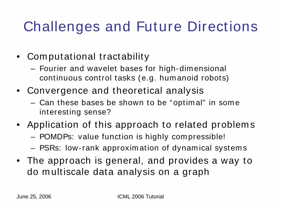
Challenges and Future Directions

• Computational tractability– Fourier and wavelet bases for high-dimensional

continuous control tasks (e.g. humanoid robots)

• Convergence and theoretical analysis– Can these bases be shown to be “optimal” in some

interesting sense?

• Application of this approach to related problems– POMDPs: value function is highly compressible!– PSRs: low-rank approximation of dynamical systems

• The approach is general, and provides a way to do multiscale data analysis on a graph


Factored and Relational MDPs

• Much work on factored and relational MDPs and RL– [Koller and Parr, UAI 2000; Guestrin et al,

IJCAI 2003; JAIR 2003 ]– [Fern, Yoon, and Givans, NIPS 2003]– ICML 2004 workshop on relational RL

• How to construct Fourier and wavelet bases over relational representations?– Symmetries and group automorphisms


Exploiting Symmetriesto Reduce Basis Size

• A graph automorphism h is a mapping from the vertex set V → V, such that– w(u,v) > 0 ↔ w(h(u),h(v)) > 0

• The automorphisms of a graph can generate compact bases

• Let P be a permutation matrix such that A P = P A

• If x is an eigenvalue of A, then so is PxA P x = P A x = λ P x


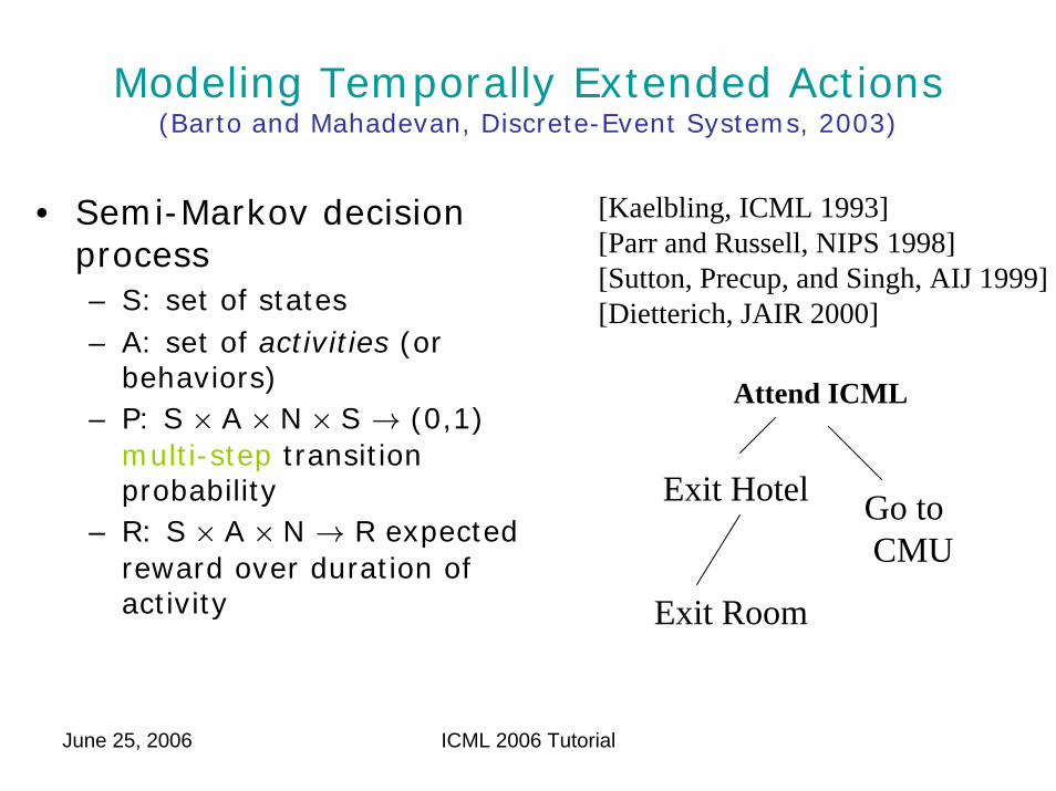
Modeling Temporally Extended Actions(Barto and Mahadevan, Discrete-Event Systems, 2003)

• Semi-Markov decision process – S: set of states– A: set of activities (or

behaviors)– P: S × A × N × S → (0,1)

multi-step transition probability

– R: S × A × N → R expected reward over duration of activity

[Kaelbling, ICML 1993][Parr and Russell, NIPS 1998][Sutton, Precup, and Singh, AIJ 1999][Dietterich, JAIR 2000]

Attend ICML

Exit Room

Exit Hotel Go toCMU


How to Discover Temporal Abstractions?

• Much recent work– Find bottlenecks and symmetries in state spaces– [McGovern, U.Mass PhD, 2002; Balaraman, U.Mass, PhD 2004]

– Rank state variables by rate of change– [Hengst, ICML 2002]

– Graph-based approaches– [Menache et al, ECML 2002; Simsek, Wolfe, and Barto, ICML

2005]

• Lacks formal framework that generalizes to arbitrary (continuous or discrete) spaces

• Does not yield compact representations of temporally extended actions


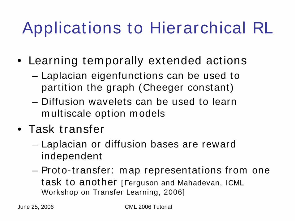
Applications to Hierarchical RL

• Learning temporally extended actions– Laplacian eigenfunctions can be used to

partition the graph (Cheeger constant)– Diffusion wavelets can be used to learn

multiscale option models

• Task transfer– Laplacian or diffusion bases are reward

independent– Proto-transfer: map representations from one

task to another [Ferguson and Mahadevan, ICML Workshop on Transfer Learning, 2006]

42

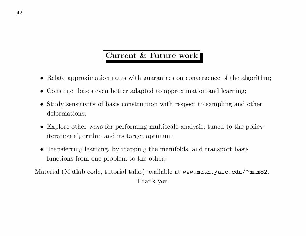
Current & Future work

• Relate approximation rates with guarantees on convergence of the algorithm;

• Construct bases even better adapted to approximation and learning;

• Study sensitivity of basis construction with respect to sampling and other

deformations;

• Explore other ways for performing multiscale analysis, tuned to the policy

iteration algorithm and its target optimum;

• Transferring learning, by mapping the manifolds, and transport basis

functions from one problem to the other;

Material (Matlab code, tutorial talks) available at www.math.yale.edu/∼mmm82.

Thank you!


Outline




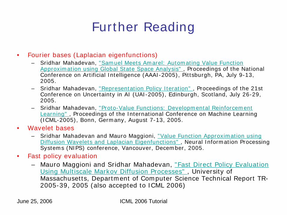
Further Reading

• Fourier bases (Laplacian eigenfunctions)– Sridhar Mahadevan, "Samuel Meets Amarel: Automating Value Function

Approximation using Global State Space Analysis" , Proceedings of the National Conference on Artificial Intelligence (AAAI-2005), Pittsburgh, PA, July 9-13, 2005.

– Sridhar Mahadevan, "Representation Policy Iteration" , Proceedings of the 21st Conference on Uncertainty in AI (UAI-2005), Edinburgh, Scotland, July 26-29, 2005.

– Sridhar Mahadevan, "Proto-Value Functions: Developmental Reinforcement Learning" , Proceedings of the International Conference on Machine Learning (ICML-2005), Bonn, Germany, August 7-13, 2005.

• Wavelet bases – Sridhar Mahadevan and Mauro Maggioni, "Value Function Approximation using

Diffusion Wavelets and Laplacian Eigenfunctions" , Neural Information Processing Systems (NIPS) conference, Vancouver, December, 2005.

• Fast policy evaluation– Mauro Maggioni and Sridhar Mahadevan, "Fast Direct Policy Evaluation

Using Multiscale Markov Diffusion Processes" , University of Massachusetts, Department of Computer Science Technical Report TR-2005-39, 2005 (also accepted to ICML 2006)

http://www.cs.umass.edu/~mahadeva/papers/aaai-final-paper.pdf



http://www.cs.umass.edu/~mahadeva/papers/final-paper.pdf



http://www.cs.umass.edu/~mahadeva/papers/nips-paper1-v5.pdf

http://www.cs.umass.edu/~mahadeva/papers/nips-paper1-v5.pdf

http://www.cs.umass.edu/~mahadeva/papers/nips-paper2-tr.pdf

http://www.cs.umass.edu/~mahadeva/papers/nips-paper2-tr.pdf


Acknowledgements

• National Science Foundation • Autonomous Learning Lab, U.Mass

– Kimberly Ferguson, Jeff Johns, Sarah Osentoski, Chang Wang

• Yale Applied Math Department– Ronald Coifman

learning representation & behavior - umass...

Documents