learning rules with adaptor grammars

Learning rules with Adaptor Grammars

Mark Johnson

joint work with Sharon Goldwater and Tom Griffiths

November 2009

1 / 81

The drunk under the lamppost

Late one night, a drunk guy is crawling around under alamppost. A cop comes up and asks him what he’s doing.

“I’m looking for my keys,” the drunk says. “I lost themabout three blocks away.”

“So why aren’t you looking for them where you droppedthem?” the cop asks.

The drunk looks at the cop, amazed that he’d ask soobvious a question. “Because the light is so much betterhere.”

2 / 81

Ideas behind talk• Statistical methods have revolutionized computational

linguistics and cognitive science• But most successful learning methods are parametric

I learn values of parameters of a fixed number of elements• Non-parametric Bayesian methods can learn the elements as

well as their weights• Adaptor Grammars use grammars to specify possible elements

I Adaptor Grammar learns probability of each adapted subtree itgenerates

I simple “rich get richer” learning rule• Applications of Adaptor Grammars:

I acquisition of concatenative morphologyI word segmentation (precursor of lexical acquisition)I learning the structure of named-entity NPs

• Sampling (instead of EM) is a natural approach to AdaptorGrammar inference

3 / 81

Language acquisition as Bayesian inference

P(Grammar | Data)︸︷︷︸Posterior

∝ P(Data | Grammar)︸︷︷︸Likelihood

P(Grammar)︸︷︷︸Prior

• Likelihood measures how well grammar describes data

• Prior expresses knowledge of grammar before data is seenI can be very specific (e.g., Universal Grammar)I can be very general (e.g., prefer shorter grammars)

• Posterior is a distribution over grammarsI captures learner’s uncertainty about which grammar is correct

4 / 81

Outline

Probabilistic Context-Free Grammars

Chinese Restaurant Processes

Adaptor grammars

Adaptor grammars for unsupervised word segmentation

Bayesian inference for adaptor grammars

Conclusion

Extending Adaptor Grammars

5 / 81

Probabilistic context-free grammars• Rules in Context-Free Grammars (CFGs) expand nonterminals

into sequences of terminals and nonterminals

• A Probabilistic CFG (PCFG) associates each nonterminal witha multinomial distribution over the rules that expand it

• Probability of a tree is the product of the probabilities of therules used to construct it

Rule r θr Rule r θrS→ NP VP 1.0NP→ Sam 0.75 NP→ Sandy 0.25VP→ barks 0.6 VP→ snores 0.4

P

Sam

NP

S

VP

barks

= 0.45 P

Sandy

NP

S

VP

snores

= 0.1

6 / 81

Learning syntactic structure is hard

• Bayesian PCFG estimation works well on toy data

• Results are disappointing on “real” dataI wrong data?I wrong rules?

(rules in PCFG are given a priori; can we learn them too?)• Strategy: study simpler cases

I Morphological segmentation (e.g., walking = walk+ing)I Word segmentation of unsegmented utterances

7 / 81

A CFG for stem-suffix morphology

Word → Stem Suffix Chars → CharStem → Chars Chars → Char CharsSuffix → Chars Char → a | b | c | . . .

Word

Stem

Chars

Char

t

Chars

Char

a

Chars

Char

l

Chars

Char

k

Suffix

Chars

Char

i

Chars

Char

n

Chars

Char

g

Chars

Char

#

• Grammar’s trees can representany segmentation of words intostems and suffixes

⇒ Can represent true segmentation

• But grammar’s units ofgeneralization (PCFG rules) are“too small” to learn morphemes

8 / 81

A “CFG” with one rule per possible morpheme

Word → Stem SuffixStem → all possible stemsSuffix → all possible suffixes

Word

Stem

t a l k

Suffix

i n g #

Word

Stem

j u m p

Suffix

#

• A rule for each morpheme⇒ “PCFG” can represent probability of each morpheme

• Unbounded number of possible rules, so this is not a PCFGI not a practical problem, as only a finite set of rules could

possibly be used in any particular data set

9 / 81

Maximum likelihood estimate for θ is trivial

• Maximum likelihood selects θ that minimizes KL-divergencebetween model and training data W distributions

• Saturated model in which each word is generated by its own rulereplicates training data distribution W exactly

⇒ Saturated model is maximum likelihood estimate

• Maximum likelihood estimate does not find any suffixes

Word

Stem

# t a l k i n g

Suffix

#

10 / 81

Forcing generalization via sparse Dirichlet priors• Idea: use Bayesian prior that prefers fewer rules• Set of rules is fixed in standard PCFG estimation,

but can “turn rule off” by setting θA→β ≈ 0• Dirichlet prior with αA→β ≈ 0 prefers θA→β ≈ 0

0

1

2

3

4

5

0 0.2 0.4 0.6 0.8 1

P(θ 1

|α)

Rule probability θ1

α = (1,1)α = (0.5,0.5)

α = (0.25,0.25)α = (0.1,0.1)

11 / 81

Morphological segmentation experiment

• Trained on orthographic verbs from U Penn. Wall StreetJournal treebank

• Uniform Dirichlet prior prefers sparse solutions as α→ 0

• Gibbs sampler samples from posterior distribution of parsesI reanalyses each word based on parses of the other words

12 / 81

Posterior samples from WSJ verb tokensα = 0.1 α = 10−5 α = 10−10 α = 10−15

expect expect expect expectexpects expects expects expects

expected expected expected expectedexpecting expect ing expect ing expect ing

include include include includeincludes includes includ es includ esincluded included includ ed includ ed

including including including includingadd add add add

adds adds adds add sadded added add ed added

adding adding add ing add ingcontinue continue continue continue

continues continues continue s continue scontinued continued continu ed continu ed

continuing continuing continu ing continu ingreport report report report

reports report s report s report sreported reported reported reported

reporting report ing report ing report ingtransport transport transport transport

transports transport s transport s transport stransported transport ed transport ed transport ed

transporting transport ing transport ing transport ingdownsize downsiz e downsiz e downsiz e

downsized downsiz ed downsiz ed downsiz eddownsizing downsiz ing downsiz ing downsiz ing

dwarf dwarf dwarf dwarfdwarfs dwarf s dwarf s dwarf s

dwarfed dwarf ed dwarf ed dwarf edoutlast outlast outlast outlas t

outlasted outlast ed outlast ed outlas ted

13 / 81

Log posterior for models on token data

-1.2e+06

-1e+06

-800000

1e-20 1e-10 1

log

P(Pa

rses

| α)

Dirichlet prior parameter α

Null suffixesTrue suffixes

Posterior

• Correct solution is nowhere near as likely as posterior

⇒ model is wrong!14 / 81

Relative frequencies of inflected verb forms

15 / 81

Types and tokens• A word type is a distinct word shape

• A word token is an occurrence of a word

Data = “the cat chased the other cat”

Tokens = “the”, “cat”, “chased”, “the”, “other”, “cat”

Types = “the”, “cat”, “chased”, “other”

• Estimating θ from word types rather than word tokenseliminates (most) frequency variation

I 4 common verb suffixes, so when estimating from verb typesθSuffix→i n g # ≈ 0.25

• Several psycholinguists believe that humans learn morphologyfrom word types

• Adaptor grammar mimics Goldwater et al “Interpolatingbetween Types and Tokens” morphology-learning model

16 / 81

Posterior samples from WSJ verb typesα = 0.1 α = 10−5 α = 10−10 α = 10−15

expect expect expect exp ectexpects expect s expect s exp ects

expected expect ed expect ed exp ectedexpect ing expect ing expect ing exp ectinginclude includ e includ e includ einclude s includ es includ es includ es

included includ ed includ ed includ edincluding includ ing includ ing includ ing

add add add addadds add s add s add sadd ed add ed add ed add ed

adding add ing add ing add ingcontinue continu e continu e continu econtinue s continu es continu es continu escontinu ed continu ed continu ed continu ed

continuing continu ing continu ing continu ingreport report repo rt rep ort

reports report s repo rts rep ortsreported report ed repo rted rep orted

report ing report ing repo rting rep ortingtransport transport transport transporttransport s transport s transport s transport stransport ed transport ed transport ed transport ed

transporting transport ing transport ing transport ingdownsize downsiz e downsi ze downsi zedownsiz ed downsiz ed downsi zed downsi zeddownsiz ing downsiz ing downsi zing downsi zing

dwarf dwarf dwarf dwarfdwarf s dwarf s dwarf s dwarf sdwarf ed dwarf ed dwarf ed dwarf ed

outlast outlast outlas t outla stoutlasted outlas ted outla sted

17 / 81

Log posterior of models on type data

-400000

-200000

0

1e-20 1e-10 1

log

P(Pa

rses

| α)

Dirichlet prior parameter α

Null suffixesTrue suffixes

Optimal suffixes

• Correct solution is close to optimal at α = 10−3

18 / 81

Desiderata for an extension of PCFGs

• PCFG rules are “too small” to be effective units ofgeneralization⇒ generalize over groups of rules⇒ units of generalization should be chosen based on data

• Type-based inference mitigates over-dispersion⇒ Hierarchical Bayesian model where:

I context-free rules generate typesI another process replicates types to produce tokens

• Adaptor grammars:I learn probability of entire subtrees (how a nonterminal expands

to terminals)I use grammatical hierarchy to define a Bayesian hierarchy, from

which type-based inference emerges

19 / 81

Outline



Adaptor grammars



Conclusion


20 / 81

Dirichlet-Multinomials with many outcomes

• Dirichlet prior α, observed data z = (z1, . . . , zn)

P(Zn+1 = k | z,α) ∝ αk + nk(z)

• Consider a sequence of Dirichlet-multinomials where:I total Dirichlet pseudocount is fixed α =

∑mk=1 αk, and

I prior uniform over outcomes 1, . . . ,m, so αk = α/mI number of outcomes m→∞

P(Zn+1 = k | z, α) ∝

nk(z) if nk(z) > 0

α/m if nk(z) = 0

But when m� n, most k are unoccupied (i.e., nk(z) = 0)

⇒ Probability of a previously seen outcome k ∝ nk(z)Probability of an outcome never seen before ∝ α

21 / 81

From Dirichlet-multinomials to Chinese

Restaurant Processes• Observations z = (z1, . . . , zn) ranging over outcomes 1, . . . ,m

• Outcome k observed nk(z) times in data z

• Predictive distribution with uniform Dirichlet prior:

P(Zn+1 = k | z) ∝ nk(z) + α/m

• Let m→∞

P(Zn+1 = k | z) ∝ nk(z) if k appears in z

P(Zn+1 6∈ z | z) ∝ α

• If outcomes are exchangable ⇒ number in order of occurence⇒ Chinese Restaurant Process

P(Zn+1 = k | z) ∝{nk(z) if k ≤ m = max(z)α if k = m+ 1

22 / 81

Chinese Restaurant Process (0)

• Customer→ table mapping z =

• P(z) = 1

• Next customer chooses a table according to:


23 / 81


α

• Customer→ table mapping z = 1

• P(z) = α/α



24 / 81


1 α

• Customer→ table mapping z = 1, 1

• P(z) = α/α× 1/(1 + α)



25 / 81


2 α

• Customer→ table mapping z = 1, 1, 2

• P(z) = α/α× 1/(1 + α)× α/(2 + α)



26 / 81


2 1 α

• Customer→ table mapping z = 1, 1, 2, 1

• P(z) = α/α× 1/(1 + α)× α/(2 + α)× 2/(3 + α)



27 / 81

Labeled Chinese Restaurant Process (0)

• Table→ label mapping y =

• Customer→ table mapping z =

• Output sequence x =

• P(x) = 1

• Base distribution P0(Y ) generates a label yk for each table k

• All customers sitting at table k (i.e., zi = k) share label yk• Customer i sitting at table zi has label xi = yzi

28 / 81


fish

α

• Table→ label mapping y = fish

• Customer→ table mapping z = 1

• Output sequence x = fish

• P(x) = α/α× P0(fish)



29 / 81


fish

1 α

• Table→ label mapping y = fish

• Customer→ table mapping z = 1, 1

• Output sequence x = fish,fish

• P(x) = P0(fish)× 1/(1 + α)



30 / 81


fish

2

apple

α

• Table→ label mapping y = fish,apple


• Output sequence x = fish,fish,apple

• P(x) = P0(fish)× 1/(1 + α)× α/(2 + α)P0(apple)



31 / 81


fish

2

apple

1 α

• Table→ label mapping y = fish,apple


• Output sequence x = fish,fish,apple,fish

• P(x) = P0(fish)× 1/(1 + α)× α/(2 + α)P0(apple)× 2/(3 + α)



32 / 81

Summary: Chinese Restaurant Processes

• Chinese Restaurant Processes (CRPs) generalizeDirichlet-Multinomials to an unbounded number of outcomes

I concentration parameter α controls how likely a new outcome isI CRPs exhibit a rich get richer power-law behaviour

• Labeled CRPs use a base distribution to label each tableI base distribution can have infinite supportI concentrates mass on a countable subsetI power-law behaviour ⇒ Zipfian distributions

33 / 81

Nonparametric extensions of PCFGs

• Chinese restaurant processes are a nonparametric extension ofDirichlet-multinomials because the number of states (occupiedtables) depends on the data

• Two obvious nonparametric extensions of PCFGs:I let the number of nonterminals grow unboundedly

– refine the nonterminals of an original grammare.g., S35 → NP27 VP17

⇒ infinite PCFGI let the number of rules grow unboundedly

– “new” rules are compositions of several rules from originalgrammar

– equivalent to caching tree fragments⇒ adaptor grammars

• No reason both can’t be done together . . .

34 / 81

Outline



Adaptor grammars



Conclusion


35 / 81

Adaptor grammars: informal description

• The trees generated by an adaptor grammar are defined byCFG rules as in a CFG

• A subset of the nonterminals are adapted

• Unadapted nonterminals expand by picking a rule andrecursively expanding its children, as in a PCFG

• Adapted nonterminals can expand in two ways:I by picking a rule and recursively expanding its children, orI by generating a previously generated tree (with probability

proportional to the number of times previously generated)

• Implemented by having a CRP for each adapted nonterminal

• The CFG rules of the adapted nonterminals determine the basedistributions of these CRPs

36 / 81

Adaptor grammar for stem-suffix morphology (0)

Word→ Stem Suffix

Stem→ Phoneme+

Suffix→ Phoneme?

Generated words:37 / 81

Adaptor grammar for stem-suffix morphology (1a)

Word→ Stem Suffix

Stem→ Phoneme+

Suffix→ Phoneme?


Adaptor grammar for stem-suffix morphology (1b)

Word→ Stem Suffix

Stem→ Phoneme+

Suffix→ Phoneme?


Adaptor grammar for stem-suffix morphology (1c)

Word→ Stem Suffix

Stem→ Phoneme+Stem

c a t

Suffix→ Phoneme?Suffix

s


Adaptor grammar for stem-suffix morphology (1d)

Word→ Stem SuffixWord

Stem

c a t

Suffix

s


c a t


s

Generated words: cats41 / 81

Adaptor grammar for stem-suffix morphology (2a)


Stem

c a t

Suffix

s


c a t


s


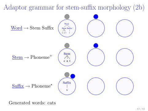
Adaptor grammar for stem-suffix morphology (2b)


Stem

c a t

Suffix

s


c a t


s


Adaptor grammar for stem-suffix morphology (2c)


Stem

c a t

Suffix

s


c a t

Stem

d o g


s


Adaptor grammar for stem-suffix morphology (2d)


Stem

c a t

Suffix

s

Word

Stem

d o g

Suffix

s


c a t

Stem

d o g


s

Generated words: cats, dogs45 / 81

Adaptor grammar for stem-suffix morphology (3)


Stem

c a t

Suffix

s

Word

Stem

d o g

Suffix

s


c a t

Stem

d o g


s

Generated words: cats, dogs, cats46 / 81

Adaptor grammars as generative processes• The sequence of trees generated by an adaptor grammar are not

independentI it learns from the trees it generatesI if an adapted subtree has been used frequently in the past, it’s

more likely to be used again• but the sequence of trees is exchangable (important for

sampling)

• An unadapted nonterminal A expands using A→ β withprobability θA→β

• Each adapted nonterminal A is associated with a CRP (orPYP) that caches previously generated subtrees rooted in A

• An adapted nonterminal A expands:I to a subtree τ rooted in A with probability proportional to the

number of times τ was previously generatedI using A → β with probability proportional to αAθA→β

47 / 81

Properties of adaptor grammars

• Possible trees are generated by CFG rulesbut the probability of each adapted tree is learned separately

• Probability of adapted subtree τ is proportional to:I the number of times τ was seen before⇒ “rich get richer” dynamics (Zipf distributions)

I plus αA times prob. of generating it via PCFG expansion

⇒ Useful compound structures can be more probable than theirparts

• PCFG rule probabilities estimated from table labels⇒ effectively learns from types, not tokens⇒ makes learner less sensitive to frequency variation in input

48 / 81

Bayesian hierarchy inverts grammatical hierarchy

• Grammatically, a Word is composedof a Stem and a Suffix, which arecomposed of Chars

• To generate a new Word from anadaptor grammar

I reuse an old Word, orI generate a fresh one from the base

distribution, i.e., generate a Stemand a Suffix

• Lower in the tree⇒ higher in Bayesian hierarchy

Word

Stem

Chars

Char

t

Chars

Char

a

Chars

Char

l

Chars

Char

k

Suffix

Chars

Char

i

Chars

Char

n

Chars

Char

g

Chars

Char

#

49 / 81

Outline



Adaptor grammars



Conclusion


50 / 81

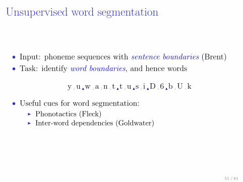
Unsupervised word segmentation

• Input: phoneme sequences with sentence boundaries (Brent)

• Task: identify word boundaries, and hence words

y Mu Nw Ma Mn Mt Nt Mu Ns Mi ND M6 Nb MU Mk

• Useful cues for word segmentation:I Phonotactics (Fleck)I Inter-word dependencies (Goldwater)

51 / 81

Word segmentation with PCFGs (1)

Sentence→Word+

Word→ Phoneme+

which abbreviates

Sentence→WordsWords→Word WordsWord→ PhonemesPhonemes→ Phoneme PhonemesPhonemes→ PhonemePhoneme→ a | . . . | z

Words

Word

Phonemes

Phoneme

D

Phonemes

Phoneme

6

Words

Word

Phonemes

Phoneme

b

Phonemes

Phoneme

U

Phonemes

Phoneme

k

52 / 81

Word segmentation with PCFGs (1)

Sentence→Word+

Word→ all possible phoneme strings

• But now there are an infinite number ofPCFG rules!

I once we see our (finite) training data,only finitely many are useful

⇒ the set of parameters (rules) should bechosen based on training data

Words

Word

D 6

Words

Word

b U k

53 / 81

Unigram word segmentation adaptor grammar

Sentence→Word+

Word→ Phoneme+

• Adapted nonterminalsindicated by underlining

Words

Word

Phonemes

Phoneme

D

Phonemes

Phoneme

6

Words

Word

Phonemes

Phoneme

b

Phonemes

Phoneme

U

Phonemes

Phoneme

k

• Adapting Words means that the grammar learns theprobability of each Word subtree independently

• Unigram word segmentation on Brent corpus: 56% token f-score

54 / 81

Adaptor grammar learnt from Brent corpus• Initial grammar

1 Sentence→Word Sentence 1 Sentence→Word1 Word→ Phons1 Phons→ Phon Phons 1 Phons→ Phon1 Phon→ D 1 Phon→ G1 Phon→ A 1 Phon→ E

• A grammar learnt from Brent corpus

16625 Sentence→Word Sentence 9791 Sentence→Word1 Word→ Phons

4962 Phons→ Phon Phons 1575 Phons→ Phon134 Phon→ D 41 Phon→ G180 Phon→ A 152 Phon→ E460 Word→ (Phons (Phon y) (Phons (Phon u)))446 Word→ (Phons (Phon w) (Phons (Phon A) (Phons (Phon t))))374 Word→ (Phons (Phon D) (Phons (Phon 6 )))372 Word→ (Phons (Phon &) (Phons (Phon n) (Phons (Phon d))))

55 / 81

Words (unigram model)

Sentence→Word+ Word→ Phoneme+

• Unigram word segmentation model assumes each word isgenerated independently

• But there are strong inter-word dependencies (collocations)• Unigram model can only capture such dependencies by

analyzing collocations as words (Goldwater 2006)

Words

Word

t e k

Word

D 6 d O g i

Word

Q t

Words

Word

y u w a n t t u

Word

s i D 6

Word

b U k

56 / 81

Collocations ⇒ Words

Sentence→ Colloc+

Colloc→Word+

Word→ Phon+

Sentence

Colloc

Word

y u

Word

w a n t t u

Colloc

Word

s i

Colloc

Word

D 6

Word

b U k

• A Colloc(ation) consists of one or more words

• Both Words and Collocs are adapted (learnt)

• Significantly improves word segmentation accuracy overunigram model (76% f-score; ≈ Goldwater’s bigram model)

57 / 81

Collocations ⇒ Words ⇒ Syllables

Sentence→ Colloc+ Colloc→Word+

Word→ Syllable Word→ Syllable SyllableWord→ Syllable Syllable Syllable Syllable→ (Onset) RhymeOnset→ Consonant+ Rhyme→ Nucleus (Coda)Nucleus→ Vowel+ Coda→ Consonant+

Sentence

Colloc

Word

Onset

l

Nucleus

U

Coda

k

Word

Nucleus

&

Coda

t

Colloc

Word

Onset

D

Nucleus

I

Coda

s

• With no supra-word generalizations, f-score = 68%• With 2 Collocation levels, f-score = 82%

58 / 81

Distinguishing internal onsets/codas helpsSentence→ Colloc+ Colloc→Word+

Word→ SyllableIF Word→ SyllableI SyllableFWord→ SyllableI Syllable SyllableF SyllableIF→ (OnsetI) RhymeFOnsetI→ Consonant+ RhymeF→ Nucleus (CodaF)Nucleus→ Vowel+ CodaF→ Consonant+

Sentence

Colloc

Word

OnsetI

h

Nucleus

&

CodaF

v

Colloc

Word

Nucleus

6

Word

OnsetI

d r

Nucleus

I

CodaF

N k

• Without distinguishing initial/final clusters, f-score = 82%• Distinguishing initial/final clusters, f-score = 84%• With 2 Collocation levels, f-score = 87%

59 / 81

Collocations2 ⇒ Words ⇒ Syllables

Sentence

Colloc2

Colloc

Word

OnsetI

g

Nucleus

I

CodaF

v

Word

OnsetI

h

Nucleus

I

CodaF

m

Colloc

Word

Nucleus

6

Word

OnsetI

k

Nucleus

I

CodaF

s

Colloc2

Colloc

Word

Nucleus

o

Word

OnsetI

k

Nucleus

e

60 / 81

Syllabification learnt by adaptor grammars

• Grammar has no reason to prefer to parse word-internalintervocalic consonants as onsets

1 Syllable→ Onset Rhyme 1 Syllable→ Rhyme

• The learned grammars consistently analyse them as eitherOnsets or Codas ⇒ learns wrong grammar half the time

Word

OnsetI

b

Nucleus

6

Coda

l

Nucleus

u

CodaF

n

• Syllabification accuracy is relatively poorSyllabification given true word boundaries: f-score = 83%Syllabification learning word boundaries: f-score = 74%

61 / 81

Preferring Onsets improves syllabification

2 Syllable→ Onset Rhyme 1 Syllable→ Rhyme

• Changing the prior to prefer word-internal Syllables withOnsets dramatically improves segmentation accuracy

• “Rich get richer” property of Chinese Restaurant Processes⇒ all ambiguous word-internal consonants analysed as Onsets

Word

OnsetI

b

Nucleus

6

Onset

l

Nucleus

u

CodaF

n

• Syllabification accuracy is much higher than without biasSyllabification given true word boundaries: f-score = 97%Syllabification learning word boundaries: f-score = 90%

62 / 81

Modelling sonority classes improves syllabification

Onset→ OnsetStop Onset→ OnsetFricative

OnsetStop → Stop OnsetStop → Stop OnsetFricative

Stop→ p Stop→ t

• Five consonant sonority classes

• OnsetStop generates a consonant cluster with a Stop at left edge

• Prior prefers transitions compatible with sonority hierarchy(e.g., OnsetStop → Stop OnsetFricative) to transitions that aren’t(e.g., OnsetFricative → Fricative OnsetStop)

• Same transitional probabilities used for initial and non-initialOnsets (maybe not a good idea for English?)

• Word-internal Onset bias still necessary

• Syllabification given true boundaries: f-score = 97.5%Syllabification learning word boundaries: f-score = 91%

63 / 81

Summary: Adaptor grammars for word

segmentation

• Easy to define adaptor grammars that are sensitive to:

Generalization Accuracywords as units (unigram) 56%+ associations between words (collocations) 76%+ syllable structure 87%

• word segmentation improves when you learn other things as well

• Adding morphology does not seem to help

64 / 81

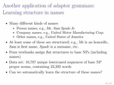
Another application of adaptor grammars:

Learning structure in names

• Many different kinds of namesI Person names, e.g., Mr. Sam Spade Jr.I Company names, e.g., United Motor Manufacturing Corp.I Other names, e.g., United States of America

• At least some of these are structured; e.g., Mr is an honorific,Sam is first name, Spade is a surname, etc.

• Penn treebanks assign flat structures to base NPs (includingnames)

• Data set: 10,787 unique lowercased sequences of base NPproper nouns, containing 23,392 words

• Can we automatically learn the structure of these names?

65 / 81

Adaptor grammar for namesNP→ Unordered+ Unordered→Word+

NP→ (A0) (A1) . . . (A6) NP→ (B0) (B1) . . . (B6)A0→Word+ B0→Word+

. . . . . .A6→Word+ B6→Word+

• Sample output:

(A0 barrett) (A3 smith)(A0 albert) (A2 j.) (A3 smith) (A4 jr.)(A0 robert) (A2 b.) (A3 van dover)(B0 aim) (B1 prime rate) (B2 plus) (B5 fund) (B6 inc.)(B0 balfour) (B1 maclaine) (B5 international) (B6 ltd.)(B0 american express) (B1 information services) (B6 co)(U abc) (U sports)(U sports illustrated)(U sports unlimited)

66 / 81

Outline



Adaptor grammars



Conclusion


67 / 81

What do we have to learn?• To learn an adaptor grammar, we need:

I probabilities of grammar rulesI adapted subtrees and their probabilities for adapted

non-terminals• If we knew the true parse trees for a training corpus, we could:

I read off the adapted subtrees from the corpusI count rules and adapted subtrees in corpusI compute the rule and subtree probabilities from these counts

– simple computation (smoothed relative frequencies)• If we aren’t given the parse trees:

I there are usually infinitely many possible adapted subtrees⇒ can’t track the probability of all of them (as in EM)

I but sample parses of a finite corpus only include finitely many

• Sampling-based methods learn the relevant subtrees as well astheir weights

68 / 81

If we had infinite data . . .

• A simple incremental learning algorithm:I Repeat forever:

– get next sentence– sample a parse tree for sentence according to current

grammar– increment rule and adapted subtree counts with counts

from sampled parse tree– update grammar according to these counts

• Particle filter learners update multiple versions of the grammarat each sentence

69 / 81

A Gibbs sampler for learning adaptor grammars

• Intuition: same as simple incremental algorithm, but re-usesentences in training data

I Assign (random) parse trees to each sentence, and computerule and subtree counts

I Repeat forever:– pick a sentence (and corresponding parse) at random– deduct the counts for the sentence’s parse from current

rule and subtree counts– sample a parse for sentence according to updated grammar– add sampled parse’s counts to rule and subtree counts

• Sampled parse trees and grammar converges to Bayesianposterior distribution

70 / 81

Sampling parses from an adaptor grammar

• Sampling a parse tree for a sentence is computationally mostdemanding part of learning algorithm

• Component-wise Metropolis-within-Gibbs sampler for parsetrees:

I adaptor grammar rules and probabilities change on the flyI construct PCFG proposal grammar from adaptor grammar for

previous sentencesI sample a parse from PCFG proposal grammarI use accept/reject to convert samples from proposal PCFG to

samples from adaptor grammar

• For particular adaptor grammars, there are often more efficientalgorithms

71 / 81

Details about sampling parses

• Adaptor grammars are not context-free

• The probability of a rule (and a subtree)can change within a single sentence

I breaks standard dynamicprogramming

• But with moderate or large corpora, theprobabilities don’t change by much

I use Metropolis-Hastings accept/rejectwith a PCFG proposal distribution

Sentence

Colloc

Word

D 6

Word

d O g i

Colloc

Word

D 6

Word

d O g i

• Rules of PCFG proposal grammar G′(t−j) consist of:I rules A→ β from base PCFG: θ′A→β ∝ αAθA→βI A rule A→ Yield(τ) for each table τ in A’s restaurant:θ′A→Yield(τ)

∝ nτ , the number of customers at table τ• Parses of G′(t−j) can be mapped back to adaptor grammar

parses72 / 81

Summary: learning adaptor grammars• Naive integrated parsing/learning algorithm:

I sample a parse for next sentenceI count how often each adapted structure appears in parse

• Sampling parses addresses exploration/exploitation dilemma

• First few sentences receive random segmentations⇒ this algorithm does not optimally learn from data

• Gibbs sampler batch learning algorithmI assign every sentence a (random) parseI repeatedly cycle through training sentences:

– withdraw parse (decrement counts) for sentence– sample parse for current sentence and update counts

• Particle filter online learning algorithmI Learn different versions (“particles”) of grammar at onceI For each particle sample a parse of next sentenceI Keep/replicate particles with high probability parses

73 / 81

Outline



Adaptor grammars



Conclusion


74 / 81

Summary and future work

• Adaptor Grammars (AG) “adapt” to the strings they generate

• AGs learn probability of whole subtrees (not just rules)

• AGs are non-parametric because cached subtrees depend on thedata

• AGs inherit the “rich get richer” property from ChineseRestaurant Processes

⇒ AGs generate Zipfian distributions⇒ learning is driven by types rather than tokens

• AGs can be used to describe a variety of linguistic inferenceproblems

• Sampling methods are a natural approach to AG inference

75 / 81

Outline



Adaptor grammars



Conclusion


76 / 81

Issues with adaptor grammars

• Recursion through adapted nonterminals seems problematicI New tables are created as each node is encountered top-downI But the tree labeling the table is only known after the whole

subtree has been completely generatedI If adapted nonterminals are recursive, might pick a table whose

label we are currently constructing. What then?• Extend adaptor grammars so adapted fragments can end at

nonterminals a la DOP (currently always go to terminals)I Adding “exit probabilities” to each adapted nonterminalI In some approaches, fragments can grow “above” existing

fragments, but can’t grow “below” (O’Donnell)• Adaptor grammars conflate grammatical and Bayesian

hierarchiesI Might be useful to disentangle them with meta-grammars

77 / 81

Context-free grammarsA context-free grammar (CFG) consists of:• a finite set N of nonterminals,• a finite set W of terminals disjoint from N ,• a finite set R of rules A→ β, where A ∈ N and β ∈ (N ∪W )?

• a start symbol S ∈ N .Each A ∈ N ∪W generates a set TA of trees.These are the smallest sets satisfying:• If A ∈ W then TA = {A}.• If A ∈ N then:

TA =⋃

A→B1...Bn∈RA

TreeA(TB1 , . . . , TBn)

where RA = {A→ β : A→ β ∈ R}, and

TreeA(TB1 , . . . , TBn) =

{�� PPA

t1 tn. . .:ti ∈ TBi

,i = 1, . . . , n

}The set of trees generated by a CFG is TS. 78 / 81

Probabilistic context-free grammarsA probabilistic context-free grammar (PCFG) is a CFG and a vectorθ, where:

• θA→β is the probability of expanding the nonterminal A usingthe production A→ β.

It defines distributions GA over trees TA for A ∈ N ∪W :

GA =

δA if A ∈ W∑A→B1...Bn∈RA

θA→B1...BnTDA(GB1 , . . . , GBn) if A ∈ N

where δA puts all its mass onto the singleton tree A, and:

TDA(G1, . . . , Gn)

(�� PPA

t1 tn. . .

)=

n∏i=1

Gi(ti).

TDA(G1, . . . , Gn) is a distribution over TA where each subtree ti isgenerated independently from Gi.

79 / 81

DP adaptor grammars

An adaptor grammar (G,θ,α) is a PCFG (G,θ) together with aparameter vector α where for each A ∈ N , αA is the parameter ofthe Dirichlet process associated with A.

GA ∼ DP(αA, HA) if αA > 0

= HA if αA = 0

HA =∑

A→B1...Bn∈RA

θA→B1...BnTDA(GB1 , . . . , GBn)

The grammar generates the distribution GS.One Dirichlet Process for each adapted non-terminal A (i.e.,αA > 0).

80 / 81

Recursion in adaptor grammars

• The probability of joint distributions (G,H) is defined by:

GA ∼ DP(αA, HA) if αA > 0

= HA if αA = 0

HA =∑

A→B1...Bn∈RA

θA→B1...BnTDA(GB1 , . . . , GBn)

• This holds even if adaptor grammar is recursive

• Question: when does this define a distribution over (G,H)?

81 / 81

learning rules with adaptor grammars

Documents