learning semantic definitions of information sources on ... · learning semantic definitions of...
TRANSCRIPT

PhD Dissertation
International Doctorate School in Information and
Communication Technologies
DIT - University of Trento
Learning Semantic Definitions
of Information Sources on the Internet
Mark James Carman
Advisor:
Prof. Paolo Traverso
Universita degli Studi di Trento
Co-Advisor:
Prof. Craig A. Knoblock
University of Southern California
July 2006


Abstract
The Internet is full of information sources providing many types of data
from weather forecasts to travel deals and financial information. These
sources can be accessed via web-forms, Web Services, RSS feeds and so
on. In order to make automated use of these sources, we need to model
them semantically. Writing semantic descriptions for web services is both
tedious and error prone. In this thesis I investigate the problem of au-
tomatically generating such models. I introduce a framework for learning
Datalog definitions for web sources. In order to learn these definitions, the
system actively invokes sources and compares the data they produce with
that of known sources of information. It then performs an inductive logic
search through the space of plausible source definitions in order to learn the
best possible semantic model for each new source. In the thesis I perform
an empirical evaluation of the system to demonstrate the effectiveness of
the approach to learning models of real-world web sources. I also compare
the system experimentally with another system capable of learning similar
information.
Keywords
Semantic Modeling, Inductive Learning, Information Integration


Acknowledgements
There are many people I would like to thank for their help, support and
encouragement over the last few years. First and foremost my wife Daniela,
who has looked after me through the journey that has culminated in the
writing of this thesis. I’d also like to thank Craig Knoblock for taking me
under his wing at a time when I was struggling to find motivation, and
giving me the confidence to improve my research. I thank Paolo Traverso
for his unlimited enthusiasm and for allowing me the scope to pursue my
interests.
I have been fortunate to work with many talented people at the Univer-
sity of Trento, the Center for Scientific and Technological Research (ITC-
irst) and the Information Sciences Institute (USC-ISI). There are a number
of colleagues to whom I owe my gratitude. In particular, Luciano Serafini
for teaching me to be rigorous in my research. Jose Luis Ambite for endless
conversations, encouragement and useful ideas regarding different facets of
this work. Yao-Yi Chiang for his patience and willingness to help. Snehal
Thakkar for listening to a perpetual stream of ideas that I just needed to
tell somebody. Kristina Lerman for her interest in my work. Matt Michel-
son for many useful discussions1. I would like to mention also Martin
Michalowski, Dan Goldberg, Rattapoom Tuchinda and Anon Plangrasop-
chok.
1and for his googling prowess.

This research is based upon work supported in part by the Defense
Advanced Research Projects Agency (DARPA), through the Department
of the Interior, NBC, Acquisition Services Division, under Contract No.
NBCHD030010. The U.S.Government is authorized to reproduce and dis-
tribute reports for Governmental purposes notwithstanding any copyright
annotation thereon. The views and conclusions contained herein are those
of the author and should not be interpreted as necessarily representing the
official policies or endorsements, either expressed or implied, of any of the
above organizations or any person connected with them.
6

Contents
1 Introduction 1
1.1 Abundance of Information . . . . . . . . . . . . . . . . . . 1
1.1.1 Emergence of Semi-structured Data Formats . . . . 1
1.1.2 Web Services, Web APIs . . . . . . . . . . . . . . . 2
1.2 Structured Querying . . . . . . . . . . . . . . . . . . . . . 3
1.2.1 Some Examples . . . . . . . . . . . . . . . . . . . . 4
1.2.2 Mediators . . . . . . . . . . . . . . . . . . . . . . . 5
1.2.3 Describing Sources as Views . . . . . . . . . . . . . 6
1.3 Discovering New Services . . . . . . . . . . . . . . . . . . . 7
1.3.1 Finding Services . . . . . . . . . . . . . . . . . . . . 8
1.3.2 Labeling Service Inputs and Outputs . . . . . . . . 8
1.3.3 Generating a Definition . . . . . . . . . . . . . . . . 9
2 Problem 11
2.1 A Motivating Example . . . . . . . . . . . . . . . . . . . . 11
2.2 Limiting the Problem . . . . . . . . . . . . . . . . . . . . . 13
2.2.1 Services with Internal State . . . . . . . . . . . . . 13
2.2.2 Services with Real-World Effects . . . . . . . . . . 15
2.3 Problem Formulation . . . . . . . . . . . . . . . . . . . . . 15
2.3.1 Preliminaries . . . . . . . . . . . . . . . . . . . . . 15
2.3.2 Definition . . . . . . . . . . . . . . . . . . . . . . . 17
2.4 Implicit Assumptions . . . . . . . . . . . . . . . . . . . . . 18
i

2.4.1 Type Signature is Known . . . . . . . . . . . . . . 18
2.4.2 Relational Flattening . . . . . . . . . . . . . . . . . 19
2.4.3 Domain Model Sufficiency . . . . . . . . . . . . . . 20
2.5 Problem Discussion . . . . . . . . . . . . . . . . . . . . . . 20
2.5.1 Domain Model . . . . . . . . . . . . . . . . . . . . 20
2.5.2 Semantic Type Specificity . . . . . . . . . . . . . . 21
2.5.3 Known Sources . . . . . . . . . . . . . . . . . . . . 21
2.5.4 Example Values . . . . . . . . . . . . . . . . . . . . 22
2.5.5 Motivation . . . . . . . . . . . . . . . . . . . . . . . 22
3 Approach 23
3.1 Modeling Language . . . . . . . . . . . . . . . . . . . . . . 23
3.1.1 Select-Project Queries . . . . . . . . . . . . . . . . 24
3.1.2 Conjunctive Queries . . . . . . . . . . . . . . . . . 25
3.1.3 Aggregation . . . . . . . . . . . . . . . . . . . . . . 26
3.1.4 Disjunction & Negation . . . . . . . . . . . . . . . 28
3.1.5 Completeness . . . . . . . . . . . . . . . . . . . . . 29
3.2 Leveraging Known Sources . . . . . . . . . . . . . . . . . . 30
3.2.1 Redundancy . . . . . . . . . . . . . . . . . . . . . . 31
3.2.2 Scope . . . . . . . . . . . . . . . . . . . . . . . . . 31
3.2.3 Binding Constraints . . . . . . . . . . . . . . . . . 31
3.2.4 Composed Functionality . . . . . . . . . . . . . . . 32
3.2.5 Access Time . . . . . . . . . . . . . . . . . . . . . . 33
3.2.6 Modeling Aid . . . . . . . . . . . . . . . . . . . . . 33
4 Inducing Definitions 35
4.1 Inductive Logic Programming . . . . . . . . . . . . . . . . 35
4.1.1 FOIL and Similar Top Down Systems . . . . . . . . 36
4.1.2 Applicability of Such Systems . . . . . . . . . . . . 37
4.2 Search . . . . . . . . . . . . . . . . . . . . . . . . . . . . . 39
ii
4.2.1 Basic Algorithm . . . . . . . . . . . . . . . . . . . . 39
4.2.2 Generating Candidates . . . . . . . . . . . . . . . . 41
4.2.3 Domain Predicates vs. Source Predicates . . . . . . 43
4.3 Limiting the Search . . . . . . . . . . . . . . . . . . . . . . 45
4.3.1 Clause Length . . . . . . . . . . . . . . . . . . . . . 46
4.3.2 Predicate Repetition . . . . . . . . . . . . . . . . . 47
4.3.3 Existential Quantification Level . . . . . . . . . . . 47
4.3.4 Executability . . . . . . . . . . . . . . . . . . . . . 48
4.3.5 Variable Repetition . . . . . . . . . . . . . . . . . . 49
4.4 Enhancements . . . . . . . . . . . . . . . . . . . . . . . . . 49
4.4.1 High Arity Predicates . . . . . . . . . . . . . . . . 50
4.4.2 Favouring Shorter Definitions . . . . . . . . . . . . 51
5 Scoring Definitions 53
5.1 Comparing Candidates . . . . . . . . . . . . . . . . . . . . 53
5.1.1 Evaluation Function . . . . . . . . . . . . . . . . . 53
5.1.2 An Example . . . . . . . . . . . . . . . . . . . . . . 55
5.2 Partial Definitions . . . . . . . . . . . . . . . . . . . . . . 57
5.2.1 Using the Projection . . . . . . . . . . . . . . . . . 57
5.2.2 Penalising Partial Definitions . . . . . . . . . . . . 58
5.3 Binding Constraints . . . . . . . . . . . . . . . . . . . . . . 61
5.3.1 Sampling . . . . . . . . . . . . . . . . . . . . . . . 61
5.3.2 Distortion . . . . . . . . . . . . . . . . . . . . . . . 62
5.4 Approximating Equality . . . . . . . . . . . . . . . . . . . 64
5.4.1 Error Bounds . . . . . . . . . . . . . . . . . . . . . 64
5.4.2 String Distance Metrics . . . . . . . . . . . . . . . 65
5.4.3 Specialized Procedures . . . . . . . . . . . . . . . . 65
5.4.4 Relation Dependent Equality . . . . . . . . . . . . 66
5.4.5 Non-Logical Equality . . . . . . . . . . . . . . . . . 67
iii

6 Optimisations & Extensions 69
6.1 Logical Optimisations . . . . . . . . . . . . . . . . . . . . . 69
6.1.1 Preliminaries . . . . . . . . . . . . . . . . . . . . . 69
6.1.2 Preventing Redundant Definitions . . . . . . . . . . 70
6.1.3 Inspecting the Unfolding . . . . . . . . . . . . . . . 73
6.1.4 Functional Sources . . . . . . . . . . . . . . . . . . 75
6.2 Constants . . . . . . . . . . . . . . . . . . . . . . . . . . . 77
6.3 Post-Processing . . . . . . . . . . . . . . . . . . . . . . . . 79
6.3.1 Tightening by Removing Redundancies . . . . . . . 79
6.3.2 Tightening based on Functional Dependencies . . . 80
6.3.3 Loosening Definitions . . . . . . . . . . . . . . . . . 81
6.4 Heuristics . . . . . . . . . . . . . . . . . . . . . . . . . . . 83
6.4.1 Type-based Predicate Ordering . . . . . . . . . . . 83
6.4.2 Look-ahead Predicate Ordering . . . . . . . . . . . 84
7 Implementation Issues 87
7.1 Generating Inputs . . . . . . . . . . . . . . . . . . . . . . . 87
7.1.1 Selecting Constants . . . . . . . . . . . . . . . . . . 87
7.1.2 Assembling Tuples . . . . . . . . . . . . . . . . . . 88
7.2 Dealing with Sources . . . . . . . . . . . . . . . . . . . . . 89
7.2.1 Caching . . . . . . . . . . . . . . . . . . . . . . . . 89
7.2.2 Source Idiosyncrasies . . . . . . . . . . . . . . . . . 90
7.3 Problem Specification . . . . . . . . . . . . . . . . . . . . . 92
7.3.1 Semantic Types, Relations & Comparison Predicates 92
7.3.2 Sources, Functions & Target Predicates . . . . . . . 93
8 Related Work 95
8.1 An Early Approach . . . . . . . . . . . . . . . . . . . . . . 95
8.2 Machine Learning Approaches . . . . . . . . . . . . . . . . 97
8.2.1 Classifying Service Inputs and Outputs . . . . . . . 97
iv

8.2.2 Classifying Service Operations . . . . . . . . . . . . 97
8.2.3 Unsupervised Clustering of Services . . . . . . . . . 98
8.3 Database Approaches . . . . . . . . . . . . . . . . . . . . . 99
8.3.1 Multi-Relational Schema Mapping . . . . . . . . . . 99
8.3.2 Schema Matching with Complex Types . . . . . . . 100
8.4 Semantic Web Approach . . . . . . . . . . . . . . . . . . . 101
8.4.1 Semantic Web Services . . . . . . . . . . . . . . . . 101
9 Evaluation 105
9.1 Experimental Setup . . . . . . . . . . . . . . . . . . . . . . 105
9.1.1 Implementation . . . . . . . . . . . . . . . . . . . . 105
9.1.2 Domains and Sources Used . . . . . . . . . . . . . . 106
9.1.3 System Settings . . . . . . . . . . . . . . . . . . . . 106
9.1.4 Evaluation Criteria . . . . . . . . . . . . . . . . . . 108
9.2 Experiments . . . . . . . . . . . . . . . . . . . . . . . . . . 109
9.2.1 Geospatial Sources . . . . . . . . . . . . . . . . . . 109
9.2.2 Financial Sources . . . . . . . . . . . . . . . . . . . 113
9.2.3 Weather Sources . . . . . . . . . . . . . . . . . . . 114
9.2.4 Hotel Sources . . . . . . . . . . . . . . . . . . . . . 116
9.2.5 Cars and Traffic Sources . . . . . . . . . . . . . . . 117
9.2.6 Overall Results . . . . . . . . . . . . . . . . . . . . 118
9.3 Empirical Comparison . . . . . . . . . . . . . . . . . . . . 119
9.3.1 iMAP: Schema Matching with Complex Types . . . 119
9.3.2 Experiments . . . . . . . . . . . . . . . . . . . . . . 119
10 Discussion 123
10.1 Contribution . . . . . . . . . . . . . . . . . . . . . . . . . . 123
10.1.1 Key Benefits . . . . . . . . . . . . . . . . . . . . . . 123
10.2 Application Scenarios . . . . . . . . . . . . . . . . . . . . . 124
10.2.1 Mining the Web . . . . . . . . . . . . . . . . . . . . 124
v

10.2.2 Real-time Source Discovery . . . . . . . . . . . . . 125
10.2.3 User Assisted Source Discovery . . . . . . . . . . . 126
10.3 Opportunities for Further Research . . . . . . . . . . . . . 126
10.3.1 Improving the Search . . . . . . . . . . . . . . . . . 126
10.3.2 Enriching the Domain Model . . . . . . . . . . . . 127
10.3.3 Extending the Query Language . . . . . . . . . . . 128
Bibliography 131
A Definitions & Derivations 137
A.1 Relational Operators . . . . . . . . . . . . . . . . . . . . . 137
A.2 Search space size . . . . . . . . . . . . . . . . . . . . . . . 137
B Experiment Data 141
B.1 Example Problem Specification . . . . . . . . . . . . . . . 141
B.2 Target Predicates . . . . . . . . . . . . . . . . . . . . . . . 141
B.3 Unfolding the Definitions . . . . . . . . . . . . . . . . . . . 143
vi

List of Tables
5.1 Examples of the Jaccard Similarity score . . . . . . . . . . 55
9.1 Inductive bias used in the experiments . . . . . . . . . . . 107
9.2 Equality procedures used in the experiments . . . . . . . . 107
9.3 Search details for geospatial problems . . . . . . . . . . . . 112
9.4 Search details for financial problems . . . . . . . . . . . . . 113
9.5 Search details for weather problems . . . . . . . . . . . . . 116
9.6 Search details for hotel problems . . . . . . . . . . . . . . 117
9.7 Search details for car and traffic problems . . . . . . . . . 118
9.8 Search details for cricket problems . . . . . . . . . . . . . . 121
vii


Chapter 1
Introduction
1.1 Abundance of Information
Recent years have seen an explosion in the quantity and variety of informa-
tion available online. One can find shopping data (prices and availability of
goods), geospatial data (such as weather forecasts, housing information),
travel data (such as flight pricing and status), financial data (exchange
rates and stock quotes), and that’s just scratching the surface of what is
available. The aim of this thesis is to make as much of that vast amount
of information available for structured querying as possible.
1.1.1 Emergence of Semi-structured Data Formats
As the amount of information has increased, so too has its reuse across
web portals and applications. Web developers and publishers soon realised
the need to manage the content of the information separately from the
presentational aspects (such as the font being used to render it). That
realisation lead to the development of XML1 and XML Schema (XML’s
type definition language) as a standard way for formatting data in a self-
1XML stands for eXtensible Markup Language.
1

1.1. ABUNDANCE OF INFORMATION CHAPTER 1. INTRODUCTION
describing manner2. In XML, metadata tags describe the data at each node
of a (semi-structured) document tree. Data structured in this manner is far
easier to manipulate than the same data hidden inside an HTML document.
Thus making it easy to integrate data from different sources, without first
needing to extract the data from the web pages containing it. Providing
the consumer of the data understands the schema (metadata tags) used in
the XML document, they can integrate the data directly into their portal
or application.
Given that the data is now available in a self describing data format, it
may even be possible to discover it in some automated fashion and integrate
it as required into an existing application. Following that path one soon
runs into the schema matching problem [25], where heterogeneity in the
metadata tags and the node structure used to describe the data must be
resolved. (Underlying semantic differences in the data itself such as the
precision of the data may also need to be reconciled.) Schema matching is
an open problem and an active area of research in the Database community.
1.1.2 Web Services, Web APIs
Building on methods for formatting data, a number of standards have
been developed for describing interfaces and providing access to that data.
These efforts are commonly referred to as Web Service standards. The
two most common protocols used for accessing web services are SOAP3,
where both the input and output of the service is encoded in an XML
message, and REST4, where the input attributes are encoded in the URL
and the output is an XML document, (RSS5 feeds often follow this pattern).
2Alternative methods for formatting data in a self describing manner in widespread use are JSON
(JavaScript Object Notation) and CSV (comma-separated values).3SOAP was originally an acronym for Simple Object Access Protocol4REST stands for Representational State Transfer5RSS is sometimes referred to as Really Simple Syndication
2

CHAPTER 1. INTRODUCTION 1.2. STRUCTURED QUERYING
Due to their simplicity, REST-based services have become very common,
especially among large portals such as Amazon, Ebay and Yahoo, which
provide programming level access to the functionality available on their
sites. Web developers for their part, have been taking advantage of these
APIs to create all sorts of Mash-Ups6 by combining content from different
sites. In general the Web is becoming programmable and web sites are
providing access to the information they contain.
Standards also exist for the definition of service interfaces7. For SOAP-
based services the interface definition language is called WSDL8, while
for REST-based services a number of competing standards for interface
definition are currently under development9. Whatever the standard, these
languages allow service providers to describe syntactically the operations
they provide in terms of what input each operation expects and what
output it will produce.
1.2 Structured Querying
Given all of the services furnishing structured data out there, one would
like to access and combine this information to provide useful information to
users. Moreover, one would like to do that not in a static/once-off fashion
as is the case for the Mash-Ups being developed, but rather in a dynamic
way as and when the specific data is being requested by the user.
6On the Internet, a Mash-Up is a website which combines the functionality of other websites, e.g. by
placing the house listings from one site on top of maps from another site.7Other Web Service standards exist that deal with authentication, non-repudiation, workflow, etc.8Web Service Description Language9See for instance WRDL, WADL and WDL.
3

1.2. STRUCTURED QUERYING CHAPTER 1. INTRODUCTION
1.2.1 Some Examples
Dynamic data requests from a user can be expressed as queries over the
data sources. Such queries may combine information from sources in ways
that were not envisaged by the producers of the original information, yet
are extremely useful to the users of it. Some simple example queries that
users might come up with are shown below. We note that the data required
to answer these queries is all publicly available and online, albeit disperse
in various data formats across multiple sources. The aim of this thesis is
to make that sort of information more readily available.
1. Tourism:
Get prices and availability for all 3* hotels within 100 miles of Trento,
Italy that lie within 1 mile of a ski resort that has over 3ft of snow.
2. Transportation:
What time do I need to leave work to catch a bus to the airport to
pick up my brother who is arriving on Qantas flight 205?
3. Disaster Prevention:
Find phone numbers for all people living within one kilometer of the
coast and below 100 meters of elevation.
4. Public Health:
Get the location of all buildings constructed before 1970 that have
more than 2 storeys and lie within 2 miles of any earthquake of mag-
nitude greater than 5.0 that occurred last week.
All of these queries require accesses to multiple data sources. It should
be clear even from this small set of examples just how useful and powerful
the ability to automatically combine data from disparate sources can be.
The queries expressed in natural language above cannot be used by an
automated system until they are expressed more formally using a query
4

CHAPTER 1. INTRODUCTION 1.2. STRUCTURED QUERYING
language such as SQL or Datalog. In Datalog the first query might be
written as follows:
q(hotel, price) :-
accommodation(hotel, 3*, address), available(hotel, today, price),
distance(address, 〈Trento,Italy〉, dist1), dist1 < 100mi,
skiResort(resort, loc1), distance(address, loc1, dist2),
dist2 < 1mi, snowCondiditions(resort, today, height),
height > 3ft.
The above expression states that hotel and price pairs are generated by
first looking up 3* hotels in a relational table called accommodation, then
checking the price for tomorrow night in a table called available. The
address of the hotel is then input to a function which calculates the distance
from Trento. The query restricts this distance to be less than 100 miles.
The query then checks that there exists a resort in the table skiResort that
lies within 1 mile of the hotel. Finally it checks the snowConditions for
today, requiring that the height of snow be greater than 3 feet.
1.2.2 Mediators
A system capable of generating a plan to answer such a query is called
an Information Mediator [2]. Mediators take queries and look for relevant
sources of information in order to answer them. A plan for answering
the first query described above might involve accesses to three different
information sources:
1. Call the Italian tourism website to find all hotels near ‘Trento, Italy’
2. Calls to a ski search engine which returns ski resorts near each hotel
3. Calls to a weather information provider to find out how much snow
has fallen at each ski resort
5

1.2. STRUCTURED QUERYING CHAPTER 1. INTRODUCTION
1.2.3 Describing Sources as Views
In order for an Information Mediator to know whether a source is relevant
for a given query, it needs to know what sort of information each source
provides. While XML defines the syntax (formatting) of the information
provided provided by a source, the semantics (intended meaning) of that
information needs to be defined separately. One way to do that is by using
a view definition in Datalog. When the view definitions have the same
form as the query shown previously, they are referred to as Local-as-View
(LAV) source definitions [13]. In effect, the source definitions describe
queries that would return the same data as the source provides. Below
are a few examples of LAV source definitions. The first definition states
that the source hotelSearch requires four values as input (input attributes
are prefixed by the $-symbol), namely a location, distance, star rating and
date. The source then produces a list of hotels which lie within the given
distance of the given location. For each hotel it returns the address of
the hotel as well as the price for a room on the given date. Note that
the relation country states that the source provides information only for
locations in Italy.
hotelSearch($location, $distance, $rating, $date, hotel, address, price) :-
country(location, Italy), accommodation(hotel, rating, address),
available(hotel, date, price), distance(address, location, dist1),
dist1 < distance.
findSkiResorts($address, $distance, resort, location) :-
skiResort(resort, location), distance(address, location, dist1),
dist1 < distance.
getSkiConditions($resort, $date, height) :-
snowCondiditions(resort, date, height).
In order to generate a plan to answer a query such as the one shown
6

CHAPTER 1. INTRODUCTION 1.3. DISCOVERING NEW SERVICES
previously, a mediator performs a process called query reformulation [13],
whereby it searches through the definitions of the available sources to see
which ones are relevant for answering the query. A source is relevant if it
refers to the same relational tables as the query. It then transforms the
query from a query over those tables to a query over the relevant sources.
For our example, the plan generated by the mediator is shown below. The
complexity of query reformulation is known to be exponential in the length
of the query and the number of sources, although efficient algorithms for
performing query reformulation do exist [23].
q(hotel, price) :-
hotelSearch(〈Trento,Italy〉, 100mi, 3*, today, hotel, address, price),
findSkiResorts(address, 1mi, resort, location),
getSkiConditions(resort, today, height), height > 3ft.
The question we are interested with in this thesis is where did all the
definitions for these information sources come from and more precisely,
what happens when we want to add new sources to the system? Is it
possible to generate some of these source definitions automatically?
1.3 Discovering New Services
In the previous example, the system knew of a sufficient number of sources
with the desired scope to be able to successfully answer the query. What
would have happened if one of the services didn’t have the desired scope,
say for example that the getSkiConditions source didn’t cover that area of
Europe? Before being able to answer the query the system would of course
need to discover a source capable of providing that kind of information. In
this section we discuss the problem of discovering new sources.
7
1.3. DISCOVERING NEW SERVICES CHAPTER 1. INTRODUCTION
1.3.1 Finding Services
As the number and variety of information sources on the Internet increases,
we will rely on automated methods for discovering them and annotating
them with semantic definitions such as those in section 1.2.3.
In order to discover relevant services, a system might search the listings
of a service registry, such as those defined in UDDI10, or perhaps more
likely, the system might search via keyword over web indices such as Google
or del.icio.us.
The research community have looked at the problem of discovering rel-
evant services. There has been some work on using service meta-data to
classify web services into different domains [11] such as weather and flights.
There has also been work on clustering similar services together [9], and
then using these clusters to improve keyword based search.
Using these techniques one can state that a new service is probably a
weather service and is similar to other weather services, which helps, but
is not sufficient for automating service integration.
1.3.2 Labeling Service Inputs and Outputs
Once a relevant service has been discovered, the problem shifts to that of
modeling it semantically, or in other words to generate a source definition
for it. Modeling sources by hand is a laborious process, so automating
the process as much as possible makes sense. Since different services often
provide similar or overlapping data, it should be possible to use knowledge
of previously modeled services to learn descriptions for newly discovered
services.
The first step in the process of modeling a particular source is to de-
termine what type of data it requires as input and what type of data it
10Universal Description, Discovery and Integration
8
CHAPTER 1. INTRODUCTION 1.3. DISCOVERING NEW SERVICES
produces as output. The research community has investigated this prob-
lem, which can essentially be viewed as a classification problem. In [11],
the authors proposed a system for classifying the attributes of a service
into semantic types, such as zipcode, (as apposed to syntactic types like
integer) based on the meta-data present in a WSDL document or the la-
bels used on a web form. Their system used a combination of Naive Bayes
and SVM11 based classifiers. More recently, the authors of [12] devel-
oped a comprehensive system in which a logistic regression based classifier
was first used to assign semantic types to input parameters of operations
in WSDL documents. Following this initial classification, the system at-
tempts to execute the operations using input values taken from examples
of the assigned semantic types. If the operation invokes correctly, then the
assignment of semantic types to the input parameters is verified. At that
point, the system takes the output values produced by the invocations, and
uses a pattern language based classifier to assign the output parameters to
certain semantic types. The authors argue that performing classification
based on both data and metadata is far more accurate that performing
classification based on the metadata alone.
For the purposes of this thesis, I assume that the problem of determining
the semantic types of the inputs and outputs of a source has been solved.
1.3.3 Generating a Definition
Once we know the semantic types for the inputs, we can invoke the service,
but we will still not be able to make use of the data it returns. To do
that, we need also to know how the output attributes relate to the input,
i.e. a view definition for the source. For example, a weather service may
return a temperature value when queried with a zipcode. The service is not
useful until we know whether the temperature being returned is the current
11SVM stands for Support Vector Machine.
9

1.3. DISCOVERING NEW SERVICES CHAPTER 1. INTRODUCTION
temperature, the predicted high temperature for tomorrow, or the average
temperature for this time of year. These different relationships between
input and output might be described by the following view definitions:
source($zip, temperature) :- currentTemp(zip, temperature).
source($zip, temperature) :- forecast(zip, tomorrow, temperature).
source($zip, temperature) :- averageTemp(zip, today, temperature).
The semantic relationships or domain relations currentTemp, forecast
and averageTemp would be defined in a domain ontology or schema. In
this thesis I describe a system capable of learning which if any of these
definitions is the correct. The system leverages what it knows about the
domain, i.e. the domain ontology and a set of known information sources,
to learn what it doesn’t know, namely the relationship between the inputs
and outputs of a newly discovered source.
So to summarise, in this thesis I investigate the problem of automatically
generating semantic descriptions for newly discovered information sources.
10

Chapter 2
Problem
In this chapter, I describe more formally the problem that is the focus of
this thesis, namely that of inducing source definition for newly discovered
services. In order to give the reader some intuition, I first give a concrete
example of the problem. I then describe some limitations on the scope of
this work. Finally I present a formal definition of the Source Definition
Induction Problem, and argue why the problem as posed is both realistic
and interesting.
2.1 A Motivating Example
As outlined in the introduction, I am interested in learning definitions
for sources by invoking them and comparing the output they produce with
that of other known sources of information. In this section I give a concrete
example of what is meant by learning a source definition.
In the example there are four types of data, namely: zipcodes, distances,
latitudes and longitudes, each of which represents its own semantic type.
There are three known sources of information. Each of the sources has
a definition in Datalog as shown below. The first service, aptly named
source1, takes in a zipcode and returns the latitude and longitude coordi-
11

2.1. A MOTIVATING EXAMPLE CHAPTER 2. PROBLEM
nates of its centroid. The second service calculates the great circle distance1
between two pairs of coordinates, while the third service converts a distance
from kilometres into miles by multiplying the input by the constant 1.6093.
source1($zip, lat, long) :- centroid(zip, lat, long).
source2($lat1, $long1, $lat2, $long2, dist) :-
greatCircleDist(lat1, long1, lat2, long2, dist).
source3($dist1, dist2) :- multiply(dist1, 1.6093, dist2).
The goal in this example is to learn a definition for a new service, called
source4, which has just been discovered on the Internet. This new service
takes in two zipcodes as input and returns a distance value:
source4($zip, $zip, dist)
The system described in this thesis, takes this type signature and searches
for appropriate definitions for the source. The definition discovered in this
case might be the following conjunction of calls to the individual sources:
source4($zip1, $zip2, dist):-
source1(zip1, lat1, long1), source1(zip2, lat2, long2),
source2(lat1, long1, lat2, long2, dist2), source3(dist2, dist).
The definition states that source’s output distance can be calculated from
the input zipcodes, by first feeding those zipcodes into source1, taking
the resulting coordinates and calculating the distance between them using
source2, and then converting that distance into miles using source3.
To test whether this source definition is correct the system would have to
invoke both the new source and the definition to see if the values generated
agree with each other. The following table shows such a test:
$zip1 $zip2 dist (actual) dist (predicted)
80210 90266 842.37 843.65
60601 15201 410.31 410.83
10005 35555 899.50 899.21
1The great circle distance is the distance around the globe between two points on the earth’s surface.
12

CHAPTER 2. PROBLEM 2.2. LIMITING THE PROBLEM
In the table, the input zipcodes have been selected randomly from a set
of examples, and the output from the source and the definition are shown
side by side. Since the output values are quite similar, once the system has
seen a sufficient number of examples, it can be confident that it has found
the correct semantic definition for the new source.
While the definition given above was written in terms of the source
relations, it could just as easily have been rewritten in terms of the domain
relations (the relations used in the definitions for sources 1 to 3). To
convert the definition into that form, one simply needs to replace each
source relation by its definition as follows:
source4($zip1, $zip2, dist):-
centroid(zip1, lat1, long1), centroid(zip2, lat2, long2),
greatCircleDist(lat1, long1, lat2, long2, dist2),
multiply(dist1, 1.6093, dist2).
Written in this way, the newly discovered semantic definition for the source
makes sense at an intuitive level: The source is simply calculating the
distance in miles between the centroids of the two zipcodes.
2.2 Limiting the Problem
As the title suggests, in this thesis I only deal with information producing
services. Many services available on the Internet either maintain some sort
of internal state, or their invocation has some effect on the “real world”.
In the following I give examples of such services and describe why I do not
deal with them directly.
2.2.1 Services with Internal State
Some of the services available online change their behaviour based on an
internal state which can be controlled by the user. For example, an oper-
13

2.2. LIMITING THE PROBLEM CHAPTER 2. PROBLEM
ation of Amazon’s API allows you to add or delete items from a shopping
cart. Describing such an operation requires the ability to describe UP-
DATE semantics, which is beyond the expressive power of the Datalog
style source definitions shown previously.
Reasoning over more expressive languages than Datalog is not at all
trivial. The fact that the system querying the sources is then able to
change the set of tuples that each relation contains, (i.e. change the state
of the system), means that query reformulation algorithms cannot be used.
Instead, systems which can reason over individual tuples produced by the
sources must be employed. AI planning systems are capable of performing
such reasoning. Since knowledge of certain types of information (such
as the winning bid price on a particular Ebay auction) will necessarily
be incomplete in the initial state, Knowledge-Level Planning capabilities
[21] would be required. Moreover, the fact that the set of values may
not or cannot by known in advance (such as the name of every product
in the Amazon catalogue), means that the planner needs the ability to
reason about partial knowledge over sets of objects (the cardinality of which
is unknown). Such a capability is beyond the current state-of-the-art in
AI planning research, although some researchers are currently working on
systems (such as [22]) with the intention of one day handling such problems.
Thus learning such definitions in terms of these more expressive lan-
guages would not only be extremely difficult to do, but would also be of
little use until planners evolve to a point in which they can handle such
definitions directly. We ought note here that certain services which may
appear “stateful” (such as login operations), may indeed not be, because
the “state” of the service is made explicit in the invocation of operations
through the passing of state variables (such as authorisation tokens). Such
services can be modeled in datalog without needing to extend the repre-
sentation.
14
CHAPTER 2. PROBLEM 2.3. PROBLEM FORMULATION
2.2.2 Services with Real-World Effects
Even more difficult to deal with than services which change their behaviour
based on an internal state, are services whose invocation affects the real
world in some way. For example, a purchase operation at an online retailer
will result in a credit card account being debited and the product being
delivered. Another operation might print pdf documents for a fee. For ob-
vious reasons, I do not attempt to learn definitions for services which affect
the world. Moreover, services with real world effects will be (or should be)
password protected, thus the system described in this thesis ought not be
able to accidentally invoke them while trying to learn a definition!
2.3 Problem Formulation
Having limited the problem to that of information providing services, I
now describe the Source Definition Induction Problem more formally.
2.3.1 Preliminaries
Before defining the problem I need to introduce some concepts and nota-
tion:
• The domain of a semantic data-type t, denoted D[t], is the (possi-
bly infinite) set of constant values {c1, c2, ...}, which constitute the
set of values for variables of that type. For example D[zipcode] =
{90210, 90292, ...}
• An attribute is a pair 〈label, semantic data-type〉, e.g. 〈zip1, zipcode〉.
The type of an attribute a is denoted type(a) and the corresponding
domain D[type(a)] is abbreviated to D[a].
15

2.3. PROBLEM FORMULATION CHAPTER 2. PROBLEM
• A scheme is an ordered (finite) set of attributes 〈a1, ..., an〉 with unique
labels, where n is referred to as the arity of the scheme. An example
scheme might be 〈zip1 : zipcode, zip2 : zipcode, dist : distance〉.
The domain of a scheme A, denoted D[A], is the cross-product of the
domains of the attributes in the scheme {D[a1]× ...×D[an]}, ai ∈ A.
• A tuple over a scheme A is an element from the set D[A]. A tuple
can be represented by a set of name-value pairs, such as {zip1 =
90210, zip2 = 90292, dist = 8.15}
• A relation is a named scheme, such as airDistance(zip1, zip2, dist).
Multiple relations may share the same scheme.
• An extension of a relation r, denoted E [r], is a subset of the tuples2 in
D[r]. For example, E [airDistance] might be a table containing the
distance between all zipcodes in California.
• A database instance over a set of relations R, denoted I[R], is a set
of extensions {E [r1], ..., E [rn]}, one for each relation r ∈ R.
• A query language L is a formal language for constructing queries over
a set of relations. We denote the set of all queries that can be writ-
ten using the language L over the set of relations R returning tuples
conforming to a scheme A as LR,A.
• The result set produced by the execution of a query q ∈ LR,A on a
database instance I[R] is denoted EI [q].
• A source is a relation s, with a binding pattern βs ⊆ s, which distin-
guishes input attributes, and a view definition, denoted vs, which is a
query written in some language LR,s. The output attributes of a source
are denoted by the complement of the binding pattern3, βcs = s\βs.
2Note that the extension of a relation may only contain distinct tuples.3The ‘\’-symbol denotes set difference.
16

CHAPTER 2. PROBLEM 2.3. PROBLEM FORMULATION
2.3.2 Definition
The Source Definition Induction Problem is defined as a tuple:
〈T, R,L, S, s∗〉
where T is a set of semantic data-types, R is a set of relations, L is a query
language, S is a set of known sources, and s∗ is the target or unknown
source.
Each semantic type t ∈ T must be provided with a set of examples values
Et ⊆ D[t]. We do not require the entire set D[t], because the domain
of many types is too large to be enumerated in the problem definition.
(For example, the semantic type zipcode has over 40,000 possible values.)
In addition a predicate eqt(t, t) is available for checking equality between
values of a given type, (to handle the case where multiple serialisations of
a variable represent the same value). In general the set of semantic types
might be arranged in a hierarchy of supertype-subtype relationships.
Each relation r ∈ R is referred to as a global relation or domain predicate,
because its extension is virtual, meaning that this extension can only be
generated by inspecting every relevant data source. (The set of relations
R may include some interpreted predicates, such as ≤, whose extension is
defined and not virtual.)
The language L used for constructing queries could be any query lan-
guage including SQL or XQuery4, but in this thesis I will be using a form
of Datalog.
Each source s ∈ S has an extension E [s] which is the complete set of
tuples that can be produced by the source (at a given moment in time). We
require that the view definition vs ∈ LR,s is consistent with the source, such
that: E [s] ⊆ EI [vs], (where I[R] is the current virtual database instance
4XQuery is an XML Query Language.
17

2.4. IMPLICIT ASSUMPTIONS CHAPTER 2. PROBLEM
over the global relations). Note that we do not require equivalence, because
some sources may provide incomplete data.
The view definition for the source to be modeled s∗ is missing. The
solution to this Source Definition Induction Problem is a new view defini-
tion v∗ ∈ LR,s∗ for the new source s∗ such that E [s∗] ⊆ EI [v∗], and there
does not exist any other view definition v′ ∈ LR,s∗, that better describes
(provides a tighter definition for) the source s∗, i.e.:
¬∃v′ ∈ LR,s∗ s.t. E [s∗] ⊆ EI [v′] ∧ |EI [v
′]| < |EI [v∗]|
I note that it may not be possible, given limitations on the computation
and bandwidth available, to guarantee that this optimality condition holds
for a particular solution found, thus in this thesis I will simply strive to
find the best solution possible, given the limitations.
2.4 Implicit Assumptions
There are a number of assumptions which are implicit in the problem for-
mulation given above. In this section I attempt to make those assumptions
explicit.
2.4.1 Type Signature is Known
The first assumption made in this work is that there exists a system capa-
ble of discovering new sources and more importantly classifying (to good
accuracy) the semantic types of their input and output. Systems capable of
performing this classification (such as [11] and [12]) were discussed briefly
in section 1.3.2.
18

CHAPTER 2. PROBLEM 2.4. IMPLICIT ASSUMPTIONS
2.4.2 Relational Flattening
The second assumption is a little less apparent and has to do with the
representation of each source as a relational view definition, i.e. as a set of
tuples conforming to given relation. Most sources on the Internet provide
tree structured data in XML. It may not always be obvious how best to
flatten that data into a set of relational tuples. (Indeed in some cases it
may not even be possible to do so and still preserve the intended meaning
of that data.)
Consider a travel booking site which returns a set of flight options each
with a ticket number, a price and a set of flight segments which constitute
the itinerary. The price of each option may vary with the number of con-
nections, as direct flights are often sold at a higher price. One possibility
for converting this data into a set of tuples would be to break each ticket up
into individual flight segment tuples. Doing this obscures the connection
between the price of the ticket and the set of flight segments comprising
it, possibly making it difficult for a learning system to discover a definition
for the source. Another possibility would be to create one tuple for each
ticket with room for a number of flight segments up to some maximum
value. This option would create a relation of very high arity and tuples
with many null values, again making life difficult for a learning system. It
is not obvious in this case, which if either of these options is to be preferred.
This problem is mitigated by the fact that most of the data available
online can be described quite “naturally” as a set of relational tuples.
Moreover, by first solving the simpler relational problem we can gain insight
and develop techniques that can later be applied to the more difficult semi-
structured case.
19

2.5. PROBLEM DISCUSSION CHAPTER 2. PROBLEM
2.4.3 Domain Model Sufficiency
A third implicit assumption in the problem formulation is that the set
of domain relations suffices for describing the source to be modeled. For
instance, consider the case where the domain model only contains relations
useful for describing financial data, and the new source provides weather
forecasts. Obviously, the system will not be able to learn a definition
for a source that cannot be described using the relations available. This
limitation does not really present a problem for the following reason: The
user can only write structured queries using the language of the domain
model, so any sources which cannot be described using that domain model
would not be useful for answering user queries anyway.
2.5 Problem Discussion
Before proceeding, there are a number of questions which arise from the
problem formulation and which I attempt to answer in this section. At
the end of the section I also give some motivation for tackling problem as
posed.
2.5.1 Domain Model
The first question that should be considered is where the domain model
comes from. In principle, the set of semantic types and relations could
come from many places. It could be taken from standard data models for
the different domains (although they may in some cases be too detailed for
the intended purpose of the source definitions). It could also come about
through consensus or it could just be the simplest model possible which
aptly describes the set of known sources. Note that the domain model may
need to evolve over time as the set of known sources expands and sources
20

CHAPTER 2. PROBLEM 2.5. PROBLEM DISCUSSION
are discovered for which no appropriate model can be found.
2.5.2 Semantic Type Specificity
The next somewhat related question is how specific the set of semantic
types ought to be. For example, is it sufficient to have one semantic type
distance or should one distinguish between distance in meters and dis-
tance in feet? Generally speaking, a semantic type should be created for
each attribute of a source which is syntactically dissimilar to the other at-
tributes of the source. For example, a phone number and a zipcode have
very different syntax, thus operations which accept one of the types as in-
put are unlikely to accept the other. The true yardstick that ought be used
to decide whether or not two attributes should be given different semantic
types is whether or not a trained classifier would be able to distinguish the
types based on their syntax alone.
In general the more semantic types there are the harder the job of the
system classifying the input and output types, and the easier the job of
the system tasked with learning a definition for the source.
2.5.3 Known Sources
Another question to be considered is where the definitions for the known
sources come from. Initially such definitions would have to be written by
hand. As the system progresses and learns definitions for different sources,
these source descriptions could be added to the set of known sources, mak-
ing it possible to learn ever more complicated definitions starting from
simple ones.
21

2.5. PROBLEM DISCUSSION CHAPTER 2. PROBLEM
2.5.4 Example Values
Finally, in order for the system to learn a definition for a new source it
needs to be able to invoke that source and possibly other sources as well.
In order to invoke the source, examples of the input types will be required.
The bigger and more representative the set of available examples of those
input types, the more efficient and accurate will be the learning process.
An initial set of examples can be provided by whoever writes the source
definitions for the known sources. As the system learns over time, it will
generate a large number of examples of different types (as output from
various sources), so generating example values should not be a problem.
Keeping the set of examples representative of the semantic type may be
challenging however.
2.5.5 Motivation
Information Integration research has reached a point where information
mediation systems are becoming mature and usable. The need to involve
a human in the writing of source definitions is, however, the Achilles Heel
of such systems. The gains in flexibility that come with the ability to
dynamically reformulate user queries are often at least in part offset by
the time and skill required to write new definitions when incorporating
new sources into the system. Thus a system capable of learning definitions
for new sources as they are discovered (or even better: when they are
required), could expand greatly the viability of mediator-based systems.
This motivation alone seems sufficient for pursuing the problem.
22
Chapter 3
Approach
The approach taken in this thesis to learning semantic models for informa-
tion sources on the web is twofold. Firstly, I choose to model sources using
the powerful query language of conjunctive queries. Secondly, I leverage
the set of known sources in order to learn a definition for the new one. In
this chapter I describe these aspects in more detail.
3.1 Modeling Language
In this section I discuss the view definition language, L, that is used for
modeling information sources on the Internet. Importantly, this is also the
hypothesis language in which new definitions will need to be learnt. As
is often the case in machine learning, we are faced with a trade-off with
regard to the expressivity (complexity) of this language. If the hypothesis
language lacks expressivity, then we may not be able to model real services
on the Internet using it. On the other hand, if the language is overly ex-
pressive, then the space of possible hypotheses will be so large that learning
will not be feasible.
The language I choose is that of conjunctive queries in Datalog, which
is a very expressive relational query language. In the next section I argue
why a less expressive language is not sufficient for our purposes. I then
23

3.1. MODELING LANGUAGE CHAPTER 3. APPROACH
describe conjunctive queries in detail, showing that they are sufficient for
modeling most online sources. For thoroughness, I then give examples of
sources which cannot be described without employing yet more expressive
languages. (I note that restrictions on the expressiveness apply only to
the definition learnt for online sources, and not to the queries that me-
diators can perform over those sources.) Finally I discuss the problem of
incomplete sources.
3.1.1 Select-Project Queries
Researchers interested in the problem of assigning semantics to web services
[11] have investigated the problem of using Machine Learning techniques
to classify WSDL-described services (based on metadata characteristics)
into different semantic domains, such as weather and flights, and the op-
erations they provide into different classes of operation, such as weather-
Forecast and flightStatus. From a relational perspective, we can consider
the different classes of operations as relations. We could then say that a
particular source simply provides values for attributes from these relations.
For instance, consider the source definition below:
source($zip, temp) :- weatherForecast(zip, tomorrow, temp).
The source provides weather data by selecting tuples from a relational table
called weatherForecast, which have the desired zipcode and date equal to
tomorrow. This query is referred to as a select-project query1 because its
evaluation can be performed using the relational operators selection and
projection. (See appendix A.1 for a formal description of these operators.)
So far so good, we have been able to use a simple classifier to learn a
definition for the source. The limitation imposed by this simple modeling
1In SQL, select-project queries correspond to the SELECT-FROM-WHERE statement, where the
FROM field contains only one relation, and the SELECT and WHERE fields contain no aggregate
operators. I discuss aggregate operators in section 3.1.3.
24

CHAPTER 3. APPROACH 3.1. MODELING LANGUAGE
language becomes obvious however, when we consider slightly more com-
plicated sources. Take for example a source that provides the temperature
in Fahrenheit as well as Celsius. In order to model such a source using a
project-select query, we would require that the weatherForecast relation be
extended with a new attribute, the source definition becoming something
like:
source($zip, tempC, tempF):-
weatherForecast(zip, tomorrow, tempC, tempF).
The more attributes that could conceivably be returned by a weather fore-
cast operation (such as sky conditions, air pressure, even latitude and lon-
gitude coordinates), the longer the relation will need to be, to cover them
all. Ideally, we would prefer in this case to add a conversion operation
convertCtoF that makes explicit the relationship between the temperature
values, and can be reused for defining other non forecast-related sources.
If in addition the source limits its output to zipcodes in California, a rea-
sonable definition for the source might be:
source($zip, tempC, tempF):-
weatherForecast(zip, tomorrow, tempC),
convertCtoF(tempC, tempF), state(zip,California).
This definition is no longer expressed in the language of select-project
queries, because it now involves multiple relations and joins between them.
Thus from this simple example, we see that modeling services using simple
select-project queries is not sufficient for our purposes. What we need are
select-project-join queries, also referred to as conjunctive queries.
3.1.2 Conjunctive Queries
The reader has already been introduced to a number of examples of con-
junctive queries throughout the previous chapters. Conjunctive queries
25

3.1. MODELING LANGUAGE CHAPTER 3. APPROACH
form a subset of the logical query language Datalog2. They are also termed
select-project-join queries because they can be evaluated using the rela-
tional operators select, project and join3. Conjunctive queries can be de-
scribed more formally as follows:
A conjunctive query over a set of relations R is an expression of
the form4:
q(X0) :- r1(X1), r2(X2), ..., rl(Xl).
where each ri ∈ R is a relation and Xi is an ordered set of variable
names of size arity(ri). Each conjunct ri(Xi) is referred to as a
literal. The set of variables in the query, denoted vars(q) =⋃l
i=0 Xi, consist of distinguished variables X0 (from the head of the
query), and existential variables vars(q)\X0, (which only appear
in the body). A conjunctive query is said to be safe if all the
distinguished variables appear in the body, i.e. X0 ⊆⋃l
i=1 Xi.
For the remainder of this thesis, I will denote the language of conjunctive
queries by L∧. Thus the set of conjunctive queries that can be written over
relations R, returning tuples of scheme A, will be denoted L∧R,A.
3.1.3 Aggregation
Implicit in the decision to use conjunctive queries in Datalog as a modeling
language is the restriction that the source can be described without the
need for aggregate operators. Aggregate operators are any operators that
2In SQL, conjunctive queries correspond to SELECT-FROM-WHERE statements containing multiple
relations, but no aggregate operators.3The join operator takes the extension of two relations and returns the subset of cross product of
those extensions for which the common attributes have the same value. A renaming operator is also
required to fully specify conjunctive queries in terms of relational operators.4The term conjunctive comes from the fact that the comma in the body (right-hand side) of the rule
is interpreted in first order logic as a conjunction, i.e.:
∀X0 ∃Y s.t. r1(X1) ∧ r2(X2) ∧ ... ∧ rl(Xl) → q(X0) where X0 ∪ Y =⋃l
i=1Xi
26

CHAPTER 3. APPROACH 3.1. MODELING LANGUAGE
must be applied to a set of tuples at once, such as MAX (find the maximum
value from a set of values), MIN, AVG, ORDER (order the values in a set),
and so on. Datalog, being a first order language, lacks the expressive power
to describe such operators (which belong to second order logic).
Some sources on the Internet cannot be described without aggregate
operators. Consider for instance a source which takes in a set of points
(latitude and longitude coordinates) and returns the distance between each
point and the centroid of the set. If the number of points in the input is
not fixed (as is possible in XML), the definition for this source would
necessarily involve an average over the set of input tuples. In general the
system will not be able to learn definitions for any sources that produce
aggregate results (except when specific relations exist in the domain model
that implicitly denote aggregation such as the averageTemp relation from
section 1.3.3).
Similarly, one cannot express orderings over the data returned, which
becomes important when a source limits the size of the result set. For
example, consider a hotel search service which returns the 20 closest hotels
to a given location. A Datalog definition for this source might look as
follows:
hotelSearch($loc, hotel, dist) :-
accommodation(hotel, loc1), distance(loc, loc1, dist).
According to this definition, however, the source should return all of the
hotels that it knows about regardless of their distance. In Datalog one
cannot express the ordering and count limitations. Ideally, one would like
to learn an expression such as the following SQL query for describing the
source5:
SELECT d.location1, a.hotel, d.distance
5In some relational database implementations, the TOP keyword is used instead of LIMIT to get the
first set of tuples returned by a query.
27

3.1. MODELING LANGUAGE CHAPTER 3. APPROACH
FROM accommodation a, distance d
WHERE d.location1 = $loc AND a.location = d.location2
ORDER BY d.distance LIMIT 20.
The reason for not using more expressive view definition languages (such
as SQL) is that the search space associated with learning such definitions
is prohibitively large.
3.1.4 Disjunction & Negation
The second restriction placed on source descriptions is that they contain
no disjunction6. This simplifying assumption holds for most information
sources and greatly reduces the space of possible hypotheses. The restric-
tion means that one cannot learn definitions for sources whose data is best
described by a union query7, i.e. a query that combines the results from
two or more different sub-queries. For example, for a while it was com-
mon for weather services in the United States to provide forecasts for cities
in both the US and Iraq. The data provided by such a service could be
described by the union of two conjunctive source definitions as follows:
s($city,US, temp) :- forecast(city,US, tomorrow, temp).
s($city, Iraq, temp) :- forecast(city, Iraq, tomorrow, temp).
Since we do not allow disjunction in the source definition language, the
best definition that could be learnt by an induction system would be the
more general rule:
s($city, country, temp) :- forecast(city, country, tomorrow, temp).
This new rule does not restrict the domain of values for the variable coun-
try. Obviously, such a general rule is not as useful to a mediator system,
which when confronted with a request for the forecast in city in say Aus-
6Disjunction in the body (the right hand side) of a Datalog rule roughly corresponds to the use of the
UNION keyword in SQL.7It should be noted that without union queries one cannot have recursive queries either.
28

CHAPTER 3. APPROACH 3.1. MODELING LANGUAGE
tralia, would proceed to call the service, oblivious to the restriction on the
country attribute.
Similar to queries containing disjunction are queries containing nega-
tion. Again the source description language L is restricted to not include
such queries, not so much because they cause the search space to explode
(including them only increases the branching factor by a factor of two),
but because view definitions requiring negation are so rare in practice,
that including them may well simply confuse the search.
A somewhat contrived example of a source definition requiring negation
is the following. Consider a source that provides a list of all movies which
have won the Venice Film Festival, but which are not being released in the
United States8. The description for such a source might look as follows:
source(film) :-
festivalWinner(film,Venice), ¬releaseDate(film,US, date).
While the above expression makes for a perfectly reasonable query to a
mediator, it is unlikely that a service provider would create such a source,
and for that reason I do not attempt to learn such definitions.
3.1.5 Completeness
One reason why definitions requiring negated literals9 are rare in practice
is that many of the sources available online are not complete with respect
to their own best definition, and providing the negation of an incomplete
table wouldn’t make much sense! The incompleteness of sources can stem
from the fact that the domain model (the set of global relations) is not
sufficiently detailed to be able to model all sources correctly. It can also
come about because the sources themselves are noisy and missing certain
8Note that this is a different set of films from those which have been scheduled for release in the US,
but with a release date in the future.9A negated literal is a literal which is preceded by the negation symbol, e.g.:
¬releaseDate(film,US, date).
29

3.2. LEVERAGING KNOWN SOURCES CHAPTER 3. APPROACH
values. Whatever the reason, the fact that sources are modeled as incom-
plete view definitions creates two problems for a learning system. Firstly,
it cannot assume that the new source for which a definition is being learnt,
will itself be complete with respect to the best possible definition (denoted
v∗ in section 2.3.2) for it. Secondly, the other sources whose data is used
to check the generated definitions, may also be incomplete with respect to
their stated definitions.
Thus the learning system, when it discovers the best definition for a
source may not even be sure that it has found the best definition, because
the set of tuples returned by the source and the set of tuples returned by
the definition may not be exactly the same, and indeed may simply overlap
with each other. I discuss the problem of evaluating candidate definitions
given incomplete sources in section 5.
3.2 Leveraging Known Sources
The overall approach that I take to the problem of discovering semantic
definitions for new services, is to leverage as much as possible the set of
known sources, while learning a new definition. Broadly speaking, I do
this by invoking the known sources (in a methodological manner) to see if
any combination of the information they provide matches the information
provided by the new source. From a practical perspective, this means that
in order to model a newly discovered sources semantically, we require that
there be some overlap in the data being produced by the new source and
the set of known sources. One way to understand this is to consider a new
source producing weather data. If none of the known sources produce any
weather information, then there will be no way for the system to learn
whether the new source is producing historical weather data, weather fore-
casts, or even that it is describing weather at all. Given this overlapping
30

CHAPTER 3. APPROACH 3.2. LEVERAGING KNOWN SOURCES
data requirement, one might claim that there is little benefit in incorporat-
ing new sources. There are a number of reasons why this is not the case,
which I detail below.
3.2.1 Redundancy
The most obvious benefit of learning definitions for new sources is redun-
dancy. If the system is able to learn that one source provides exactly the
same information as a currently available source, then if the latter suddenly
becomes unavailable, the former can be used in its place. For example if
a mediator knows of one weather source providing current conditions, and
learns that a second source provides the same or similar data, then if the
first goes down for whatever reason (perhaps because an access quota has
been reached), weather data can still be accessed from the second.
3.2.2 Scope
The second and perhaps more interesting reason for wanting to learn a
definition for a new source is that the new source may provide data which
lies outside the scope of (or simply not present in) the data provided by
the other sources. For example, consider a weather service which provides
temperature values for zipcodes in the United States. Then consider a
second source that provides weather forecasts for cities worldwide. If the
system can use the first source to learn a definition for the second, the
amount of information available for querying suddenly increases greatly.
3.2.3 Binding Constraints
Binding constraints on a service can make accessing certain types of in-
formation difficult or inefficient. In this case, discovering a new source
providing the same or similar data but with a different binding pattern
31

3.2. LEVERAGING KNOWN SOURCES CHAPTER 3. APPROACH
may improve performance. For example, consider a hotel search web ser-
vice that accepts a zipcode and returns a set of hotels along with their star
rating and so on:
hotelSearch($zip, hotel, rating, street, city, state):-
accommodation(hotel, rating, street, city, state, zip).
Now consider a simple query for the names and addresses of all five star
hotels in California:
q(hotel, street, city, zip):-
accommodation(hotel, 5*, street, city,California, zip).
Answering this query would require thousands of calls to the known source
- one for every zipcode in California. And even then a mediator could only
answer the query if there exists another source capable of producing such a
set of zipcodes. In contrast, if the system had learnt a definition for a new
source which provides exactly the same data but with a different binding
pattern:
hotelsByState($state, $rating, hotel, street, city, zip):-
accommodation(hotel, rating, street, city, state, zip).
Then answering the same query would require only one call to this new
source!
3.2.4 Composed Functionality
Often the functionality of a complex source can be described in terms of
a composition of the functionality provided by other simpler services. For
instance, consider the motivating example from section 2.1, in which the
functionality provided by the new source was to calculate the distance in
miles between two zipcodes. The same functionality could be achieved
by performing four different calls to the available sources. In that case,
the definition learnt by the system meant that any query regarding the
distance between zipcodes could be handled more efficiently. In general,
32

CHAPTER 3. APPROACH 3.2. LEVERAGING KNOWN SOURCES
by learning definitions for more complicated sources in terms of simpler
ones, the system can benefit from computation, optimisation and caching
abilities of services providing complex functionality.
3.2.5 Access Time
Finally, the newly discovered service may be faster to access than the
known sources providing similar data. For instance, consider a geocoding
service which takes in an address and returns the latitude and longitude
coordinates of the location. Because of the variety in algorithms used
to calculate the coordinates, it’s not unreasonable for a geocoding source
to take a long time (upwards of one second) to return a result. If the
system were able to discover a new source providing the same geocoding
functionality, but with a delay of only 50 milliseconds, then the system
would be able to geocode a set of addresses 20 times faster.
3.2.6 Modeling Aid
There exist also application scenarios in which the overlapping data require-
ment discussed previously, does not pose much of a restriction. Consider
the case where a domain modeler is manually annotating the different op-
erations of a particular web service. Often the operations of a single service
simply provide different ways of accessing the same underlying data. If this
is the case, and the operations are sufficiently similar, a learning system
should be able to induce definitions for the other operations automatically,
based on the definition given for the first operation. Doing so may re-
duce the time required to model new sources and/or reduce the numbers
of errors and inconsistencies in the models produced.
33

3.2. LEVERAGING KNOWN SOURCES CHAPTER 3. APPROACH
34

Chapter 4
Inducing Definitions
In this chapter I describe an algorithm for generating candidate definitions
for a newly discovered source. The algorithm forms the first phase in
a generate and test methodology for learning source definitions. I defer
discussion of the testing phase to the next chapter.
4.1 Inductive Logic Programming
The language used to express definitions for information sources, Datalog,
is a type of first-order language. It is in fact, simply the function-free
subset of the commonly used first-order programming language Prolog. In
the Machine Learning community, systems capable of learning models us-
ing expressive first-order representations are referred to as Inductive Logic
Programming (ILP) systems or Relational Learners. Because of the expres-
sivity of the modeling language (specifically the ability to describe joins
across “hidden variables” such as the coordinates of a zipcode in the ex-
ample from section 2.1), the complexity of the relational learning problem
is much higher than for propositional rule learners (also called attribute-
value learners). The latter form the bulk of Machine Learning algorithms
including commonly used decision-tree learners, naive bayes learners and
Support Vector Machines.
35

4.1. ILP CHAPTER 4. INDUCING DEFINITIONS
Given that I model services using conjunctive Datalog queries, many of
the techniques developed for learning such first-order (relational) represen-
tations should also apply to the problem of inducing source definitions for
online sources. In the next section I introduce an ILP system and discuss
its applicability to the problem.
4.1.1 FOIL and Similar Top Down Systems
FOIL (First Order Inductive Learner) [5] is a well known ILP search algo-
rithm. It is capable of learning first-order rules to describe a target pred-
icate, which is represented by a set of positive examples (tuples over the
target relation, denoted E+) and optionally also a set of negative examples
(E−). The search for a viable definition in FOIL proceeds in a top down
manner, starting from an empty clause1 and iteratively adding literals to
the body (antecedent) of the rule, thereby making the rule more specific.
This process continues until the definition (denoted h) covers only posi-
tive examples and no negative examples. Using the notation introduced in
section 2.3.1 we could write this condition as follows:
E+ ∩ EI [h] 6= ∅ and E− ∩ EI [h] = ∅
Usually a set of rules are learnt in this manner by removing the positive
examples covered by the first rule and repeating the process. The set of
rules are interpreted as a union query which covers all the positive tuples
and none of the negative ones:
E+ ⊆⋃
i EI [hi] and E− ∩⋃
i EI [hi] = ∅
Search in FOIL is performed in a greedy best-first manner, guided by an
information-gain-based heuristic. Many extensions to the basic FOIL al-
gorithm exist, most notably those that combine declarative background1I use the terms clause and query interchangeably to refer to a conjunctive query in Datalog. An
empty clause is a query without any literals in the body (right side) of the clause.
36

CHAPTER 4. INDUCING DEFINITIONS 4.1. ILP
knowledge into the search process such as FOCL (First Order Combined
Learner) [19]. Such systems are categorised as performing a top down
search because they start from an empty clause (the most general rule pos-
sible) and specialize the clause by adding literals one at a time. Bottom up
approaches on the other hand (such as GOLEM [17]), perform a specific to
general search starting from the positive examples of the target predicate.
4.1.2 Applicability of Such Systems
There are a number of issues which limit the direct applicability of Induc-
tive Logic Programming systems to the source definition induction prob-
lem:
• Extensions of the global relations are virtual.
• Sources may be incomplete with respect to their definitions.
• Explicit negative examples of the target are not available.
• Sources may serialise constants in different ways.
The first issue has to do with the fact that all ILP systems assume that
there are extensional (or in some cases intentional) definitions of both the
target predicate and the predicates that will be used in the definition for the
target. In other words, they assume that tables already exist in some rela-
tional database to represent both the new source and the known sources.
In our case we need to generate such tables by first invoking the services
with relevant inputs. One could envisage invoking each of the sources with
every possible input and using the resulting tables to perform induction.
Such a direct approach would not be feasible for two reasons. Firstly, a
complete set of possible input values may not be known to the system. Sec-
ondly, even if it is possible to generate a complete set of viable inputs to a
service, it may not be practical to query the source with such a large set
37

4.1. ILP CHAPTER 4. INDUCING DEFINITIONS
of tuples. Consider for example source4 from section 2.1, which calculates
the distance in miles between a pair of zipcodes. Given that there are over
40,000 zipcodes in the US, generating an extensional representation of this
source would require more than one billion invocations to be performed!
Obviously performing such a large number of invocations does not make
sense when a small number of example invocations would suffice for glean-
ing the desired information regarding the characteristics of a source. In
this thesis I develop an algorithm that only queries the sources as needed
in order to evaluate individual candidate definitions.
The second issue has to do with the incompleteness of the sources. This
lack of completeness causes a problem when a candidate (h) is to be eval-
uated. Since the set of tuples returned by a source will only be a subset
of those implied by its definition, so too will be the set of tuples returned
by the candidate hypothesis when executed (as the execution must be per-
formed over those incomplete sources). This means that when the system
tries to evaluate a hypothesis by comparing the tuples it produces with
those of the source, it cannot be sure that a tuple which is produced by
the new source but is not among the the tuples representing the hypothesis
is in fact not logically implied by the hypothesis. This fact must then be
taken into account when deciding on an evaluation function for assessing
the quality of a hypothesis. I will discuss such an evaluation function in
section 5.1.1.
The third issue regarding the lack of explicit negative examples for
the target predicate also effects the evaluation of candidate hypotheses.
The classic approach to handling a lack of explicit negative examples is to
make the closed world assumption, in which all tuples (over the head rela-
tion) which are not explicitly declared to be positive are assumed negative.
Given the fact that the new source may in fact be incomplete with respect
to the best possible definition for it, the assumption that all tuples which
38

CHAPTER 4. INDUCING DEFINITIONS 4.2. SEARCH
are not returned by the source are negative examples of its definition is not
necessarily correct. In other words, just because a particular tuple is pro-
duced when the candidate definition is executed and that same tuple is not
returned by the new source does not necessarily mean that the candidate
definition is incorrect.
The fourth issue has to do with the fact that the data which is provided
by the different sources has not been cleaned, in the sense that different
serialisations (strings) may be used by different sources to represent the
same value (such as “Monday” and “Mon”) for instance. Since ILP systems
have been designed to operate over a single database containing multiple
tables, this issue of heterogeneity in the data values is not handled by
current systems. I defer discussion of how this heterogeneity is resolved to
section 5.4.
4.2 Search
In this section I describe the actual search procedure that is used to gen-
erate candidate definitions for a new source. The procedure is based on
the top-down best-first search strategy used in FOIL. Later in the section
I discuss the trade-off involved in writing definitions in terms of source
relations as opposed to global relations.
4.2.1 Basic Algorithm
The algorithm used to enumerate the space of possible view definitions
takes as input a type signature for the new source and uses it to seed the
search for candidate definitions. (In the following I will refer to the new
source relation as the target predicate and the set of known source relations
as source predicates.) The space of candidate definitions is enumerated in a
best-first manner, with each candidate being tested to see if the data it re-
39

4.2. SEARCH CHAPTER 4. INDUCING DEFINITIONS
turns is similar to the target. Pseudo-code describing the overall algorithm
is shown in algorithm 1:
input : A predicate signature s∗
output: The best scoring view definition v∗
Invoke target with set of random inputs;1
Add empty clause to queue;2
while queue 6= ∅ do3
v ← best definition from queue;4
forall v′ ∈ expand(v) do5
if eval(v′) ≥ eval(v) then6
insert v′ into queue;7
end8
end9
end10
Algorithm 1: Best-First Search Algorithm
The first step in the algorithm is to invoke the new source with a rep-
resentative set of input tuples so as to generate examples of output tuples
that characterize the functionality of the source. This set of invocations
must include positive examples (invocations for which output tuples were
produced) and if possible, also negative tuples (i.e. inputs for which no out-
put was returned). The algorithm’s ability to induce the correct definition
for a source will be highly dependent on the number of positive examples
available. Thus a minimum requirement on the number of positive invoca-
tions of the source is imposed. This means that the algorithm may have to
invoke the source repeatedly using different inputs until sufficient positive
invocations can be recorded. Selecting appropriate input values so as to
successfully invoke a service is easier said than done. I defer discussion of
the issues and difficulties involved in successfully invoking the new source
40

CHAPTER 4. INDUCING DEFINITIONS 4.2. SEARCH
to section 7.1, and assume for the moment that the induction system is
able to generate a table of values that represent its functionality.
The next step in the algorithm is to initialise the search by adding an
empty clause to the queue of definitions to expand. The rest of the algo-
rithm is simply a best-first search procedure with backtracking. At each
iteration the highest scoring but not yet expanded definitions is removed
from the queue and expanded. Each candidate generated is compared to
the original definition to see if the score is improved. If so it is added to
the queue. If no definitions are found that improve the score, backtracking
is performed. In the next section I will describe the expansion step (line 4
of the algorithm) in more detail.
4.2.2 Generating Candidates
In order to generate candidate definitions for the new source, the system
performs a top-down best-first search through the space of conjunctions of
source predicates. In other words, it starts with a very simple source defi-
nition and builds ever more complicated definitions by adding one source
predicate at a time to the end of the best definition found so far. It keeps
doing this until the data produced by the definition matches that produced
by the source it is trying to model.
I now run through an example of the process of generating candidate
definitions. Consider a newly discovered source, which takes in a zipcode
and a distance, and returns all the zipcodes that lie within the given radius
(along with their respective distances). The target predicate representing
this source is as follows:
source5($zip1, $dist1, zip2, dist2)
Now assume that there are two known sources. The first being the source
for which the definition was learnt in the example from section 2.1, namely:
41

4.2. SEARCH CHAPTER 4. INDUCING DEFINITIONS
source4($zip1, $zip2, dist):-
centroid(zip1, lat1, long1), centroid(zip2, lat2, long2),
greatCircleDist(lat1, long1, lat2, long2, dist2),
multiply(dist1, 1.6093, dist2).
The second source isn’t actually a source but is the interpreted predicate
less-than. Being interpreted, it doesn’t need a definition, as the system
knows how to check ordering over distance values. (Note that the binding
constraints for this predicate requires that both arguments be bound, which
means that the less-than predicate cannot be used to generate any values,
just check ordering over them.)
≤($dist1, $dist2).
The search for a definition for the new source might then proceed as follows.
The first definition to be generated is the empty clause:
source5($ , $ , , ).
The null character ( ) represents the fact that none of the inputs or out-
puts have any restrictions placed on their values. Prior to adding the first
literal (source predicate), the system will check whether any output at-
tributes echo the input values. In this case, given the semantic types, two
possibilities would need to be checked:
source5($zip1, $ , zip1, ).
source5($ , $dist1, , dist1).
Assuming neither of these possibilities is true (i.e. improves the score),
then literals will be added one at a time to refine the definition. A literal is
a source predicate with an assignment of variable names to its attributes.
A new definition must be created for every possible literal that includes
at least one variable already present in the clause. (For the moment I
ignore the issue of binding constraints on the sources being added and
defer discussion to section 4.3.4.) Thus many candidate definitions would
be generated including the following:
42

CHAPTER 4. INDUCING DEFINITIONS 4.2. SEARCH
source5($zip1, $dist1, , ) :- source4($zip1, $ , dist1).
source5($zip1, $ , zip2, ) :- source4($zip1, $zip2, ).
source5($ , $dist1, , dist2) :- ≤(dist1, dist2).
Note that the semantic types in the type signature of the target predicate
limit greatly the number of candidate definitions that can be produced.
The system then evaluates each of these candidates in turn, selecting the
best one for further expansion. Assuming the first of the three has the
best score, it would be expanded by adding another literal, forming more
complicated candidates such as the following:
source5($zip1, $dist1, , dist2) :-
source4($zip1, $ , dist1), ≤(dist1, dist2).
This process continues until the system discovers a definition which per-
fectly describes the source, or is forced to backtrack because no literal
improves the score.
4.2.3 Domain Predicates vs. Source Predicates
In the above example, the decision to perform search over the source pred-
icates rather than the domain predicates was made in an arbitrary fashion.
In this section I justify that decision. If one were to perform the search
over the domain predicates, then testing each definition would require an
additional query reformulation step. For example, consider the following
candidate definition for source5 containing the domain predicate centroid:
source5($zip1, $ , , ) :- centroid(zip1, , ).
In order to evaluate this candidate, the system would need to first treat
the definition as a query and reformulate it into a set of rewritings (that
together form a union query) over the various sources as follows:
source5($zip1, $ , , ) :- source4($zip1, $ , ).
source5($zip1, $ , , ) :- source4($ , $zip1, ).
This union query can then be executed against the available sources (in
43
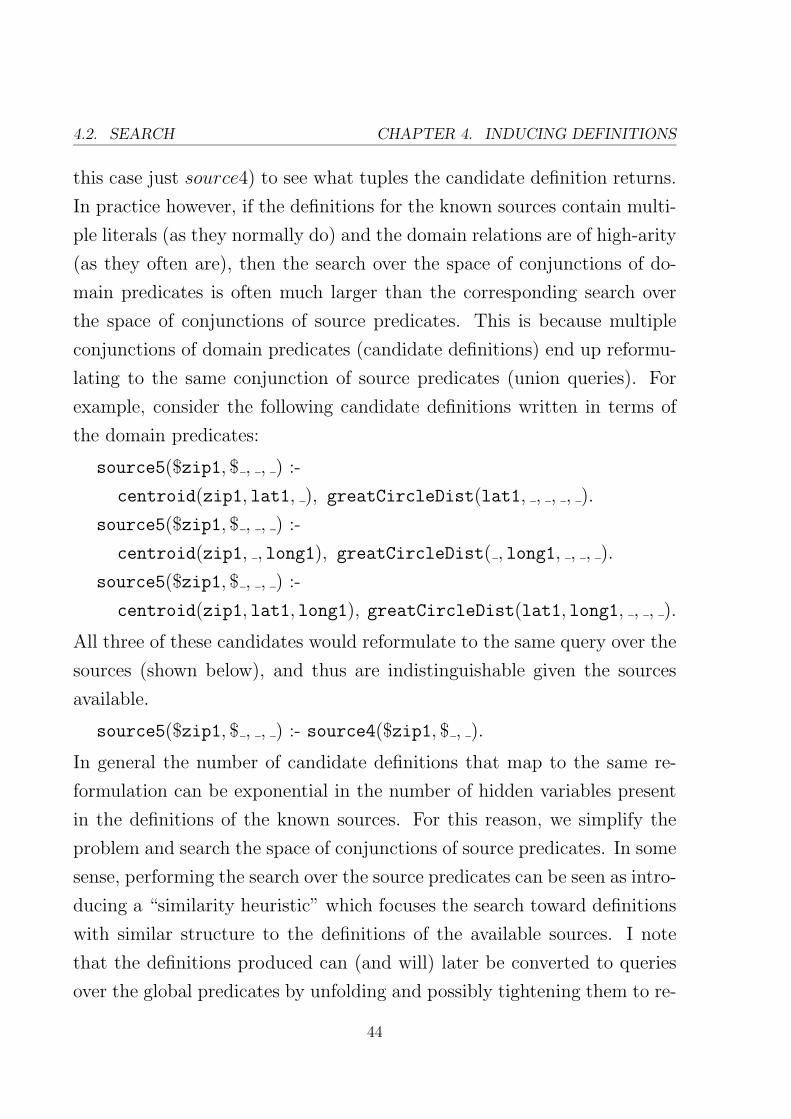
4.2. SEARCH CHAPTER 4. INDUCING DEFINITIONS
this case just source4) to see what tuples the candidate definition returns.
In practice however, if the definitions for the known sources contain multi-
ple literals (as they normally do) and the domain relations are of high-arity
(as they often are), then the search over the space of conjunctions of do-
main predicates is often much larger than the corresponding search over
the space of conjunctions of source predicates. This is because multiple
conjunctions of domain predicates (candidate definitions) end up reformu-
lating to the same conjunction of source predicates (union queries). For
example, consider the following candidate definitions written in terms of
the domain predicates:
source5($zip1, $ , , ) :-
centroid(zip1, lat1, ), greatCircleDist(lat1, , , , ).
source5($zip1, $ , , ) :-
centroid(zip1, , long1), greatCircleDist( , long1, , , ).
source5($zip1, $ , , ) :-
centroid(zip1, lat1, long1), greatCircleDist(lat1, long1, , , ).
All three of these candidates would reformulate to the same query over the
sources (shown below), and thus are indistinguishable given the sources
available.
source5($zip1, $ , , ) :- source4($zip1, $ , ).
In general the number of candidate definitions that map to the same re-
formulation can be exponential in the number of hidden variables present
in the definitions of the known sources. For this reason, we simplify the
problem and search the space of conjunctions of source predicates. In some
sense, performing the search over the source predicates can be seen as intro-
ducing a “similarity heuristic” which focuses the search toward definitions
with similar structure to the definitions of the available sources. I note
that the definitions produced can (and will) later be converted to queries
over the global predicates by unfolding and possibly tightening them to re-
44

CHAPTER 4. INDUCING DEFINITIONS 4.3. LIMITING THE SEARCH
move redundancies. I will discuss the process of tightening the unfoldings
in section 6.3.1.
4.3 Limiting the Search
The search space generated by this top-down search algorithm may be very
large even for a small number of sources. An upper bound for this space is
given by the following expression: (See Appendix A.2 for an explanation
of how this upper bound is derived.)
size(l, |S|, a) ≤l
∑
i=0
|S| + i − 1
i
B((i + 1)a)
Here l is the maximum length of the clauses generated, |S| is the number
of sources available, and a is the maximum arity of any of those sources,
(which is assumed to be greater than the arity of the target predicate).
B(n) is the nth Bell number, which is the count of all partitions2 of a set
of size n. It represents the number of different ways n variables can be
assigned names (equated) independently of the labels used [27]. The Bell
number is calculated recursively as follows:
B(0) = 1 and B(n + 1) =n
∑
k=0
n
k
B(k)
Intuitively, the set of all partitions is greater than the powerset but less
than the set of permutations, i.e.: 2n < B(n) < n! for n ≥ 5. Needless to
say, this upper bound for the search space is extremely large. It increases
in a super exponential manner with the length l and the maximum arity
a. For example, in the experiments described in chapter 9, the maximum
arity for a source predicate is 16, and there are over 30 sources, making
the search space bound enormous even for small l.
2A partition of a set X is a set of non-empty subsets {Y1, ..., Yn}, Yi ⊆ X, |Yi| > 0, which exactly
cover the set, i.e. X =⋃
i Yi and ∀i6=j Yi ∩ Yj = ∅.
45

4.3. LIMITING THE SEARCH CHAPTER 4. INDUCING DEFINITIONS
The use of semantic types limits greatly the ways in which variables
within each definition can be equated (aka the join paths) and thus goes
a long way to reduce the size of the search space. If we let b denote the
maximum number of times the same type appears in any given source
predicate, (for simplicity assume that b divides evenly into a), then the
upper bound becomes the following:
size(l, |S|, a, b) ≤l
∑
i=0
|S| + i − 1
i
B((i + 1)b)a/b
For example, if a = 16 and b = 8 then the search space for l = 0 is 611
times smaller than without semantic types.
Despite this reduction, as the number of sources available increases, the
search space becomes so large that techniques for limiting it must be used.
We employ some standard (and other not so standard) ILP techniques
for limiting this space. Such limitations are often referred to as inductive
search bias or language bias [18].
4.3.1 Clause Length
The most obvious way to limit the search space is to limit the maximum
length of a clause, i.e. the number of source predicates that can occur
in a definition. Implementing this limitation in the algorithm described
previously simply involves backtracking whenever the definition reaches
the maximum length. Such forced backtracking provides an important
way of escaping from local minima in the search space that result from the
greedy enumeration.
The assumption being made here is that shorter definitions are more
probable than longer ones, which makes sense as service providers are likely
to provide data in the simplest (rawest) form possible. Moreover, the
simpler the definition of the sources learnt, the more useful they will be
to a mediator, so it makes sense to trade away completeness (losing the
46

CHAPTER 4. INDUCING DEFINITIONS 4.3. LIMITING THE SEARCH
ability to express longer definitions) in exchange for improved accuracy
over shorter definitions.
4.3.2 Predicate Repetition
The second restriction placed on the candidate definitions is to limit the
number of times the same source predicate appears in a given candidate.
Doing this makes sense because the definitions of real services tend not
to contain many repeated predicates. Intuitively speaking, this is because
most services provide raw data without performing many calculations over
it. Repeated use of the same predicate in a definition is more useful for de-
scribing some form of calculation than raw data itself. (Exceptions to this
rule exist, for example predicates representing unit conversion functional-
ity such as Fahrenheit to Celsius, may necessarily occur multiple times in
the definition of a source.)
Limiting to one the number of times the same predicate occurs in the
body of a clause would reduce the upper bound on the search space con-
siderably:
size(l, |S|, a, b) ≤l
∑
i=0
|S|
i
B((i + 1)b)a/b
4.3.3 Existential Quantification Level
The third bias limits the complexity of the definitions generated by re-
ducing the number of literals that do not contain variables from the head
of the clause. Specifically, it limits the level of existential quantification
(sometimes also referred to as the depth [17]) of each variable in a clause.
This level is defined to be zero for all distinguished variables (those ap-
pearing in the head of the clause). For existential variables (those not
appearing in the head) it is defined recursively as one plus the lowest level
of any variable appearing in the same literal. For example, the candidate
47

4.3. LIMITING THE SEARCH CHAPTER 4. INDUCING DEFINITIONS
definition shown below has a maximum existential quantification level of
three because the shortest path from the last literal to the head literal (via
join variables) passes through two other literals:
source5($zip1, $ , , ) :-
source4($zip1, $ , d1), source3($d1, d2), source3($d2, ).
The effect of this bias is to concentrate the search around simpler but highly
connected definitions, where each literal is closely linked to the input and
output of the source. Taking this restriction to an extreme by limiting
the maximum level of a variable to be 1 (all literals must contain a head
variable), would reduce the search space to (assuming for simplicity that
b = a and that the target predicate has arity less than a):
size(l, |S|, a, b) ≤l
∑
i=0
|S|
i
B((i + 1)(a − 1))a2i
4.3.4 Executability
The fourth restriction placed on source definitions is that they are exe-
cutable. More specifically, it should be possible to execute them from left
to right, meaning that the inputs of each source appear either in the target
predicate (head of the clause) or in one of the literals to the left of that
literal. For example, of the two candidate definitions shown below, only
the first definition is executable. The second definition is not, because zip2
is used as input for source4 in the first literal, without first being bound
to a value in the head of the clause:
source5($zip1, $ , zip2, ) :- source4($zip1, $zip2, ).
source5($zip1, $ , , ) :-
source4($zip1, $zip2, dist1), source4($zip2, $zip1, dist1).
This restriction serves two purposes. Firstly, like the other biases, it limits
the size of the search space. Secondly, it makes it easier to evaluate the
definitions produced. In theory, one could still evaluate the second def-
48

CHAPTER 4. INDUCING DEFINITIONS 4.4. ENHANCEMENTS
inition above by generating lots of input values for zip2, but this would
require a lot of invocations for minimal gain. While the upper bound on
the resulting search space does not change, I note that the size of the search
space necessarily shrinks as a result of the constraints placed by binding
patterns on the types of definitions possible.
4.3.5 Variable Repetition
The last restriction reduces the search space by limiting the number of
times the same variable can appear in any given literal in the body of the
clause. Definitions in which the same variable appears multiple times in a
given literal, such as in the following example which returns the distance
between a zipcode and itself, are not very common in practice:
source5($zip1, $ , , dist2) :- source4(zip1, zip1, dist2).
If we set the maximum repetition to be zero, this definition would not be
allowed, because zip1 appears twice in the same literal. Explicitly pre-
venting such definitions from being generated makes sense because sources
requiring them are so rare, that it is better to reduce the search space
exponentially3 by ignoring them, than to explicitly check for them each
time.
4.4 Enhancements
I now discuss some enhancements to the basic search algorithm introduced
in section 4.2.1.
3The number of different ways that the variables within a literal can be assigned names in this case
reduces from B(a) to 2a.
49

4.4. ENHANCEMENTS CHAPTER 4. INDUCING DEFINITIONS
4.4.1 High Arity Predicates
The sources used in the examples of section 4.2.2 all had relatively low
arity. On the Internet this is unlikely to be the case. Moreover, a number
of those sources are likely to contain a large numbers of attributes of the
same type. This is a problem, because it will cause an exponential number
of definitions to be possible at each expansion step. Consider for instance
a service providing stock price data. A relation representing the source is
shown below. The source takes as input a ticker symbol and returns the
current price, high and low prices, as well as market opening and closing
prices:
stockprice($ticker, price, price, price, price, price)
If the definition to which this predicate is to be added already contains k
price variables, then the number of ways in which the price attributes of
the new relation can be assigned variables is∑5
i=0
(
5i
)(
k+i−1i
)
. This value is
prohibitively large number even for moderate k.
To limit the search space in the case of such high-arity predicates, we
first generate candidates with a minimal number of bound variables in
the new literal and progressively constrain the best performing of these
definitions within each expansion. (High arity predicates are handled in a
similar fashion in FOIL [24].) For example, consider using the stockprice
source above to learn a definition for a new source, with type signature:
source6($ticker, price, price)
We start by adding literals to an empty definition as before. This time
though, instead of generating a literal, for every possible assignment of
variable names to the attributes of each relation, we generate only the
simplest assignments such that all of the binding constraints are met. In
this particular example, the ticker symbol input of the stockprice source
would need to be bound, generating a single definition:
50

CHAPTER 4. INDUCING DEFINITIONS 4.4. ENHANCEMENTS
source6($tic, , ) :- stockprice($tic, , , , , ).
This definition would then be evaluated, and if it scores well, more con-
strained definitions would be generated by equating a variable from the
same literal to other variables from the clause. Two such definitions are
shown below:
source6($tic, pri1, ) :- stockprice($tic, pri1, , , , ).
source6($tic, pri1, ) :- stockprice($tic, , pri1, , , ).
The best of these definitions would then be selected and constrained fur-
ther, generating definitions such as:
source6($tic, pri1, pri2) :- stockprice($tic, , pri1, pri2, , ).
source6($tic, pri1, pri2) :- stockprice($tic, , pri1, , pri2, ).
In this way, the best scoring literal can be found without the need to iterate
over all of the possible assignments of variables to attributes.
4.4.2 Favouring Shorter Definitions
As mentioned previously, shorter definitions for the target source should
be preferred over longer and possibly less accurate ones. In accordance
with this principle, the second enhancement I make to the basic algorithm
is to weight definitions by their length so as to favour shorter definitions
as follows:
eval(v) = ωlength(v) · score(v)
Here v is the candidate definition, ω < 1 is a weighting factor, length(v)
is the length of the clause, and score is a function for evaluating clauses,
(a definition for which will be introduced in the next chapter). Setting the
weighting factor to be a little less than 1 (such as 0.95) helps to remove
logically redundant definitions, which can sometimes be hard to detect, but
are often return almost exactly the same score as their shorter equivalent.
I will discuss the problem of generating non-redundant clauses in section
51

4.4. ENHANCEMENTS CHAPTER 4. INDUCING DEFINITIONS
6.1.2.
52

Chapter 5
Scoring Definitions
In this chapter I discuss techniques for evaluating the candidate definitions
generated by the induction system.
5.1 Comparing Candidates
I now proceed to the problem of evaluating the candidate definitions gen-
erated during search. The basic idea is to compare the output produced
by the source with the output produced by the definition for the same
input. The more similar the tuples produced, the higher the score for the
candidate. The score is then averaged over a set of different input tuples
to get an indication of how well the candidate definition describes the data
produced by the new source.
5.1.1 Evaluation Function
In the motivating example of section 2.1, the source for which a definition
was being learnt (the definition is repeated below), only produced one
output tuple 〈dist〉 for every input tuple 〈zip1, zip2〉:
source4($zip1, $zip2, dist):-
centroid(zip1, lat1, long1), centroid(zip2, lat2, long2),
53
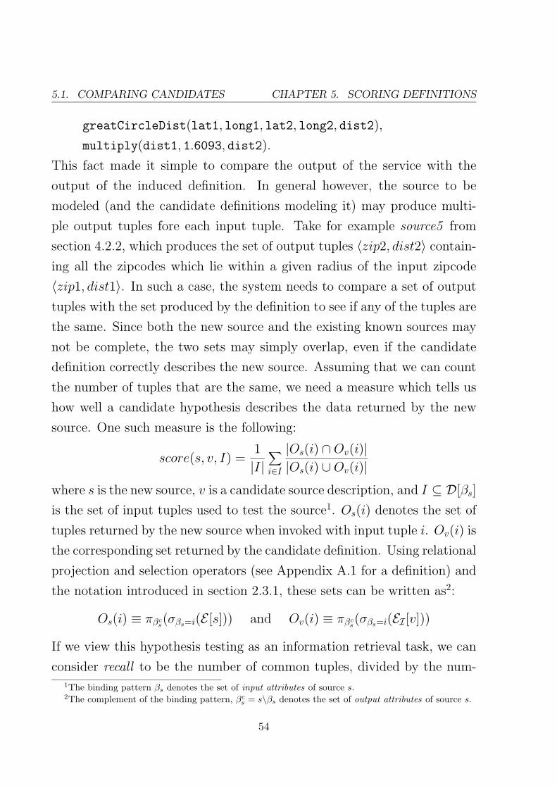
5.1. COMPARING CANDIDATES CHAPTER 5. SCORING DEFINITIONS
greatCircleDist(lat1, long1, lat2, long2, dist2),
multiply(dist1, 1.6093, dist2).
This fact made it simple to compare the output of the service with the
output of the induced definition. In general however, the source to be
modeled (and the candidate definitions modeling it) may produce multi-
ple output tuples fore each input tuple. Take for example source5 from
section 4.2.2, which produces the set of output tuples 〈zip2, dist2〉 contain-
ing all the zipcodes which lie within a given radius of the input zipcode
〈zip1, dist1〉. In such a case, the system needs to compare a set of output
tuples with the set produced by the definition to see if any of the tuples are
the same. Since both the new source and the existing known sources may
not be complete, the two sets may simply overlap, even if the candidate
definition correctly describes the new source. Assuming that we can count
the number of tuples that are the same, we need a measure which tells us
how well a candidate hypothesis describes the data returned by the new
source. One such measure is the following:
score(s, v, I) =1
|I|
∑
i∈I
|Os(i) ∩ Ov(i)|
|Os(i) ∪ Ov(i)|
where s is the new source, v is a candidate source description, and I ⊆ D[βs]
is the set of input tuples used to test the source1. Os(i) denotes the set of
tuples returned by the new source when invoked with input tuple i. Ov(i) is
the corresponding set returned by the candidate definition. Using relational
projection and selection operators (see Appendix A.1 for a definition) and
the notation introduced in section 2.3.1, these sets can be written as2:
Os(i) ≡ πβcs(σβs=i(E [s])) and Ov(i) ≡ πβc
s(σβs=i(EI [v]))
If we view this hypothesis testing as an information retrieval task, we can
consider recall to be the number of common tuples, divided by the num-1The binding pattern βs denotes the set of input attributes of source s.2The complement of the binding pattern, βc
s = s\βs denotes the set of output attributes of source s.
54

CHAPTER 5. SCORING DEFINITIONS 5.1. COMPARING CANDIDATES
ber of tuples produced by the source, and precision to be the number of
common tuples divided by the number of tuples produced by the defini-
tion. The above measure takes both precision and recall into account by
calculating the average Jaccard similarity between the sets.
5.1.2 An Example
Table 5.1 gives an example of how this score is calculated for each input
tuple.
input tuple actual output predicted output Jaccard similarity
i ∈ I tuples Os(i) tuples Ov(i) for tuple i
〈a, b〉 {〈x, y〉, 〈x, z〉} {〈x, y〉} 1/2
〈c, d〉 {〈x,w〉, 〈x, z〉} {〈x,w〉, 〈x, y〉} 1/3
〈e, f〉 {〈x,w〉, 〈x, y〉} {〈x,w〉, 〈x, y〉} 1
〈g, h〉 ∅ {〈x, y〉} 0
〈i, j〉 ∅ ∅ #undef!
Table 5.1: Examples of the Jaccard Similarity score
The first two rows of the table show inputs for which the predicted and
actual output tuples overlap with each other. In the third row, the defini-
tion produces exactly the same set of tuples as the source being modeled
and thus gets the maximum score. In the fourth row, the definition pro-
duced a tuple, while the source didn’t, so the definition was penalised. In
the last row, the definition correctly predicted that no tuples would be out-
put from the source. Our score function is undefined at this point. From
a certain perspective the definition should score well here because it has
correctly predicted that no tuples be returned for that input, but giving
a high score to a definition when it produces no tuples can be dangerous.
Doing so may cause overly constrained definitions which can generate very
few output tuples to score well, while causing less constrained definitions
that are better at predicting the output tuples on average to score poorly
55

5.1. COMPARING CANDIDATES CHAPTER 5. SCORING DEFINITIONS
overall. For example, consider a source which returns weather forecasts for
zipcodes in Los Angeles. The correct definition for this source is shown
below:
source($zip, temp) :-
forecast(zip, tomorrow, temp), UScity(zip,Los Angeles).
Now consider two candidate definitions for the source. The first returns
the temperature for a zipcode, while the second returns the temperature
only if it is below 0◦C:
v1($zip, temp) :- forecast(zip, tomorrow, temp).
v2($zip, temp) :- forecast(zip, tomorrow, temp), temp < 0 ◦C .
Assume that the source and candidates are invoked using 20 different ran-
domly selected zipcodes from all over the US. For most of these zipcodes
the source will not return any output, because the zipcode will lie outside of
Los Angeles. The first candidate will likely return output for all zipcodes,
while the second candidate would, like the source, only rarely produce any
output. This is because the temperature in most zipcodes will be greater
than zero, and has nothing to do with whether or not the zipcode is in Los
Angeles.
If we score definitions highly when they correctly produce no output,
the system would erroneously prefer the second candidate over the first,
(because the latter often produces no output). To prevent that from hap-
pening, we simply ignore inputs for which the definition correctly predicts
zero tuples. This is the same as setting the score for this case to be the
average of the other values.
Returning our attention to table 5.1, after ignoring the last row, the
overall score for this definition would be calculated as 0.46.
56

CHAPTER 5. SCORING DEFINITIONS 5.2. PARTIAL DEFINITIONS
5.2 Partial Definitions
As the search proceeds toward the correct definition for the service, many
semi-complete (unsafe) definitions will be generated. These definitions will
not produce values for all attributes of the target tuple but only a subset
of them. For example, the candidate definition:
source5($zip1, $dist1, zip2, ) :- source4(zip1, zip2, dist1).
produces only one of the two output attributes produced by the source.
This presents a problem, because our score is only defined over sets of
tuples containing all of the output attributes of the new source. One
solution might be to wait until the definitions become sufficiently long
as to produce all outputs, before comparing them to see which one best
describes the new source. There are two reasons why doing this would not
make sense:
• The space of safe definitions is too large to enumerate, and thus we
need to compare partial definitions so as to guide the search toward
the correct definition.
• The best definition that the system can generate may well be a partial
one, as the set of known sources may not be sufficient to completely
model the source.
5.2.1 Using the Projection
The simplest way to compute a score for a partial definition is to compute
the same function as before, but instead of using the raw source tuples,
projecting them over the subset of attributes that are produced by the
definition. This revised score is shown below. (Note that the projection
is over v\βs, which denotes the subset of output attributes of s which are
produced by the view definition v. Note also that the projection is not
57

5.2. PARTIAL DEFINITIONS CHAPTER 5. SCORING DEFINITIONS
distinct, i.e. multiple instances of the same tuple may be produced3.)
score′(s, v, I) =1
|I|
∑
i∈I
|πv\βs(Os(i)) ∩ Ov(i)|
|πv\βs(Os(i)) ∪ Ov(i)|
This revised score is not very useful however, as it gives an unfair advantage
to definitions that do not produce all of the output attributes of the source.
This is because it is far easier to correctly produce a subset of the output
attributes than to produce all of them. Consider for example the two source
definitions shown below. The two definitions are identical except that the
second returns the output distance value dist2, while the first does not:
source5($zip1, $dist1, zip2, ) :-
source4(zip1, zip2, dist2), ≤(dist2, dist1).
source5($zip1, $dist1, zip2, dist2) :-
source4(zip1, zip2, dist2), ≤(dist2, dist1).
Since the two are identical, the projection over the subset will in this case
return the same number of tuples. This then means that both definitions
would get the same score although the second definition is clearly better
than the first as it produces all of the required outputs.
5.2.2 Penalising Partial Definitions
We need to be able to penalise partial definitions in some way for the
attributes they don’t produce. One way to do this is to first calculate
the size of the domain |D[a]| of each of the missing attributes. In the
example above, the missing attribute is the distance value. Since distance
is a continuous value, calculating the size of its domain is not obvious. We
can approximate the size of its domain by:
|D[distance]| ≈max − min
accuracy
3The fact that the projection is not distinct is important for preserving the correctness of the calcu-
lation.
58
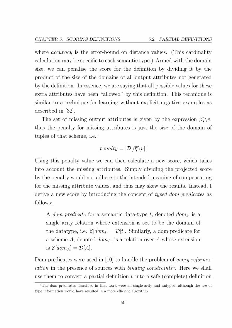
CHAPTER 5. SCORING DEFINITIONS 5.2. PARTIAL DEFINITIONS
where accuracy is the error-bound on distance values. (This cardinality
calculation may be specific to each semantic type.) Armed with the domain
size, we can penalise the score for the definition by dividing it by the
product of the size of the domains of all output attributes not generated
by the definition. In essence, we are saying that all possible values for these
extra attributes have been “allowed” by this definition. This technique is
similar to a technique for learning without explicit negative examples as
described in [32].
The set of missing output attributes is given by the expression βcs\v,
thus the penalty for missing attributes is just the size of the domain of
tuples of that scheme, i.e.:
penalty = |D[βcs\v]|
Using this penalty value we can then calculate a new score, which takes
into account the missing attributes. Simply dividing the projected score
by the penalty would not adhere to the intended meaning of compensating
for the missing attribute values, and thus may skew the results. Instead, I
derive a new score by introducing the concept of typed dom predicates as
follows:
A dom predicate for a semantic data-type t, denoted domt, is a
single arity relation whose extension is set to be the domain of
the datatype, i.e. E [domt] = D[t]. Similarly, a dom predicate for
a scheme A, denoted domA, is a relation over A whose extension
is E [domA] = D[A].
Dom predicates were used in [10] to handle the problem of query reformu-
lation in the presence of sources with binding constraints4. Here we shall
use them to convert a partial definition v into a safe (complete) definition
4The dom predicates described in that work were all single arity and untyped, although the use of
type information would have resulted in a more efficient algorithm
59

5.2. PARTIAL DEFINITIONS CHAPTER 5. SCORING DEFINITIONS
v′. We can do this simply by adding a dom predicate to the end of the
view definition that generates values for the missing attributes. For the
example above, v′ would be:
source5($zip1, $dist1, zip2, x) :-
source4(zip1, zip2, dist2), ≤(dist2, dist1), domdistance(x).
where x is a new variable of type distance. The new view definition v′
is safe, because all the variables in the head of the clause also appear in
the body. In general, we can turn an unsafe view definition v into a safe
definition v′ by appending a dom predicate domβcs\v(x1, ..., xn), where each
xi is a distinguished variable (from the head of the clause) corresponding
to an output attribute of v′ that wasn’t bound in v. Now we can use this
complete definition to calculate the score as before:
score′′(s, v, I) = score(s, v′, I) =1
|I|
∑
i∈I
|Os(i) ∩ Ov′(i)|
|Os(i) ∪ Ov′(i)|
which can be rewritten (by expanding the denominator) as follows:
score′′(s, v, I) =1
|I|
∑
i∈I
|Os(i) ∩ Ov′(i)|
|Os(i)| + |Ov′(i)| − |Os(i) ∩ Ov′(i)|
We can then remove the references to v′ from this equation by considering:
Ov′(i) = Ov(i) × E [domβcs\v] = Ov(i) ×D[βc
s\v]
Thus the size of the set is given by |Ov′(i)| = |Ov(i)||D[βcs\v]| and the size
of the intersection can be calculated (by taking the projection over the
output attributes produced by v) as follows:
|Os(i) ∩ Ov′(i)| = |πv\βs(Os(i) ∩ Ov(i) ×D[βc
s\v])| = |πv\βs(Os(i)) ∩ Ov(i)|
Substituting these cardinalities into the score function given above, we
arrive at the following equation for the penalised score:
score′′(s, v, I) =1
|I|
∑
i∈I
|πv\βs(Os(i)) ∩ Ov(i)|
|Os(i)| + |Ov(i)||D[βcs\v]| − |πv\βs
(Os(i)) ∩ Ov(i)|
60

CHAPTER 5. SCORING DEFINITIONS 5.3. BINDING CONSTRAINTS
5.3 Binding Constraints
Some of the candidates definitions generated during the search may have
different binding constraints from the target predicate. For instance in the
partial definition shown below, the variable zip2 is an output of the target
source, but an input to source4 :
source5($zip1, $dist1, zip2, ) :- source4($zip1, $zip2, dist1).
From a logical perspective, in order to test this definition correctly, we need
to invoke source4 with every possible value from the domain of zipcodes.
Doing this is not practical for two reasons: Firstly, the system may not
have a complete list of zipcodes at its disposal. Secondly and far more
importantly, invoking source4 with thousands of different zipcodes would
take a very long time and would probably result in the system being blocked
from further use of the service.
5.3.1 Sampling
So instead of invoking the same source thousands of times, we approximate
the score for this definition by sampling from the domain of zipcodes and
invoking the source using the sampled values. We then compensate for this
sampling by scaling (certain components of) the score by the ratio of the
sampled zipcodes to the entire domain. Considering the example above, if
we randomly choose a sample (denoted δ[zipcode]) of say 20 values from
the domain of zipcodes, then the set of tuples returned by the definition
will need to be scaled by a factor of |D[zipcode]|/20.
A more general equation for computing the scaling factor is shown be-
low. Note that the sampling may need to be performed over a set of
attributes (δ[βv\βs] ⊆ D[βv\βs]), where βv\βs denotes all of the input at-
tributes of the view which are outputs of the new source5.
5The executability constraint from section 4.3.4 ensures that βv ⊆ s.
61
5.3. BINDING CONSTRAINTS CHAPTER 5. SCORING DEFINITIONS
scaling =|D[βv\βs]|
|δ[βv\βs]|
I now calculate the effect of this scaling factor on the overall score as
follows. I denote the set of tuples returned by the definition given the
sampled input as Ov(i). This value when scaled will approximate the set
of tuples that would have been returned had the definition been invoked
with all the possible values for the additional input attributes:
|Ov(i)| ≈ |Ov(i)| ∗ scaling
Assuming the sampling is performed randomly over the domain of possible
values, the intersection between the tuples produced by the source and
the definition should scale in the same way. Thus the only factor not
affected by the scaling in the score defined previously is |Os(i)|. If we
divide throughout by the scaling factor we have a new score function as
follows:
1
|I|
∑
i∈I
|πv\βs(Os(i)) ∩ Ov(i)|
|Os(i)|/scaling + |Ov(i)||D[βcs\v]| − |πv\βs
(Os(i)) ∩ Ov(i)|
5.3.2 Distortion
The problem with this approach is that often the sampled set of values is
too small and as a result it does not intersect with the set of values returned
by the source, even though a larger sample would have intersected in some
way. Thus our sampling introduces unfair distortions into the score for
certain definitions causing them to perform poorly.
For example, consider again source5 and assume that for scalability
purposes, the service places a limit on the maximum value for the input
radius dist1. (This makes sense, as otherwise the user could set the input
radius to cover the entire US, and a tuple for every possible zipcode would
62

CHAPTER 5. SCORING DEFINITIONS 5.3. BINDING CONSTRAINTS
need to be returned.) Now consider the sampling performed above. If we
randomly choose only 20 zipcodes from the set of all possible zipcodes, the
chance of the sample containing a zipcode which lies within say a 300 mile
radius of a particular zipcode (in say, the middle of the desert) is very low.
Moreover, even if one pair of zipcodes (out of 20) results in a successful
invocation, this will not be sufficient for learning a good definition for the
service.
So to get around this problem I bias the sample such that, whenever
possible, half of the values are taken from positive examples of the target
(i.e. the set of tuples returned by the new source) and half are taken
from negative examples (those tuples not returned by the source). By
sampling from both positive and negative tuples, we guarantee that the
approximation generated will be as accurate as possible given the limited
sample size used.
I denote the set of positive and negative samples as δ+[βv\βs] and
δ−[βv\βs], and use these values to define scaling factors as shown below.
(The numerator for the positive values is different from before, as these
values have been taken from the output of the new source.)
scaling+ =|πβv\βs
(πv\βs(Os(i)))|
|δ+[βv\βs]|
The total scaling is the same value as before, but calculated slightly differ-
ently:
scaling =|D[βv\βs]|
|δ+[βv\βs]| + |δ−[βv\βs]|
The score can then be approximated accordingly by taking into account
these new scaling factors. Differently from before, the intersection needs
to be scaled using the positive scaling factor:
|πv\βs(Os(i)) ∩ Ov(i)| ≈ |πv\βs
(Os(i)) ∩ Ov(i)| ∗ scaling+
63

5.4. APPROXIMATING EQUALITY CHAPTER 5. SCORING DEFINITIONS
This new scaling results in a new function for evaluating the quality of a
view definition, denoted score′′′′(s, v, I):
1
|I|
∑
i∈I
|πv\βs(Os(i)) ∩ Ov(i)| ∗ scaling+
|Os(i)| + |Ov(i)||D[βcs\v]| ∗ scaling − |πv\βs
(Os(i)) ∩ Ov(i)| ∗ scaling+
5.4 Approximating Equality
Up until this point I have ignored the problem of deciding whether two
tuples produced by the target source and the definition are the same. Since
different sources may serialize data in different ways and at a different level
of accuracy, we must allow for some flexibility in the values that the tuples
contain. For instance, in the example from section 2.1, the distance values
returned by the source and definition did not match exactly, but were
“sufficiently similar” to be accepted as the same value. Defining equality
as exact string matches may make sense for certain types, such as zipcodes,
but it won’t make much sense for other types like distance, temperature or
company name.
5.4.1 Error Bounds
For numeric types like temperature or distance it makes sense to use an
error bound (like ±0.5◦C) or a percentage error (such as ±1%) to decide
if two values can be considered the same. This is because the sensing
equipment (in the case of temperature) or the algorithm used (in the case
of distance) will have some error bound associated with it the values it
produces. I require that an error bound for each numeric type be provided
in the problem specification, although the origin of that bound may be
some automated procedure which learns from examples.
64

CHAPTER 5. SCORING DEFINITIONS 5.4. APPROXIMATING EQUALITY
5.4.2 String Distance Metrics
For certain nominal types like company names, where values like 〈IBM
Corporation〉 and 〈International Business Machines Corp.〉 represent the
same value, simplistic equality checking using exact or substring matches
is not sufficient for deciding whether two values correspond to the same
entity. In this case string edit distances such as the JaroWinkler score do
a better job at distinguishing strings representing the same entity from
those representing different ones. (See [7] for a discussion and comparison
of various string similarity measures.)
A machine learning classifier could be trained on a set of such exam-
ples to learn which of the available string edit distances best distinguishes
values of that type and what threshold to set for accepting a pair as a
match. I require that this pair of similarity metric and threshold (or any
combinations of metrics) be provided in the problem specification.
5.4.3 Specialized Procedures
In other cases, an enumerated types like months of the year might be
associated with a simple equality checking procedure, so that values like
〈January〉, 〈Jan〉 and 〈1〉 can be found equal. The actual equality procedure
used will depend on the semantic type and we assume in this work that
such a procedure is given in the problem definition. We note that the
procedure need not be 100% accurate, but only provide a sufficient level
of accuracy to guide the system toward the correct source description.
Indeed, the equality rules could even be generated offline by training a
machine learning classifier.
Complex types such as date present an even bigger problem when one
considers the range of possible serializations, including values like 〈5/4/2006〉
or 〈May 4, 2006〉 or 〈Thu, 4 May 2006〉 or 〈2006-05-04〉. In such cases spe-
65

5.4. APPROXIMATING EQUALITY CHAPTER 5. SCORING DEFINITIONS
cialized functions are not only required to check equality between values
but also to break the complex types up into their constituent parts (in
this case day, month and year). The latter would form part of the domain
model.
5.4.4 Relation Dependent Equality
In some cases, deciding whether two values of the same type can be consid-
ered equal doesn’t just depend on the Semantic Type, but on the relations
they are used in as well. For instance, consider the two relations shown
below. The first provides the latitude and longitude coordinates of the cen-
troid for a zipcode, while the second returns the coordinates for a particular
address:
centroid(zipcode, latitude, longitude)
geocode(number, street, zipcode, latitude, longitude)
Given the different ways of calculating the centroid (including using the
center of mass or the center of population density) of a zipcode, an error
bound of 500 meters might make sense for equating latitude and longitude
coordinates. For a geocoding service on the other hand an error bound of
50 meters may be more reasonable.
In the general case, such error bounds should be associated with the set
of global relations instead of just the semantic types and could be learnt
accordingly. If the attributes of the relations contain multiple (nominal or
numeric) attributes, then the problem of deciding whether two tuples refer
to the same entity (are the same) is called the record linkage problem [29].
There exists an entire field of research devoted to tackling this problem.
Due to the complexity of the problem and the variety of techniques that
have been developed to handle it, I do not investigate this problem further
in this thesis.
66

CHAPTER 5. SCORING DEFINITIONS 5.4. APPROXIMATING EQUALITY
5.4.5 Non-Logical Equality
Finally, an alternative to handling equality between values of a data-type
in a purely logical manner would be to associate each pair of values with a
similarity score between zero and one (such as that returned by the edit-
distance metrics mentioned previously), and use this value to calculate the
similarity between tuples of values. In this case, one would be able to
define the similarity between two tuples (denoted τ1 and τ2) in such a way
that the similarity increases with the number of similar component values.
For instance the following equation uses a probabilistic interpretation to
calculate the similarity between tuples6 (τ1(a) denotes the value of the
attribute a in the tuple τ1):
similarity(τ1, τ2) = 1 −∏
a∈A
(1 − similarity(τ1(a), τ2(a)))
A threshold could then be applied to decide whether two tuples do refer to
the same entity. Proceeding in this manner while interesting would cause a
number of complications in the evaluation of view definitions, not the least
of which, how one should calculate joins across relations. Thus the idea
of implementing induction using similarities rather than equality is left to
future work.
6Note that the symbol∏
denotes the product not the projection, which is denoted π
67

5.4. APPROXIMATING EQUALITY CHAPTER 5. SCORING DEFINITIONS
68
Chapter 6
Optimisations & Extensions
In this chapter I discuss various optimisations and extensions to the algo-
rithm outlined in chapters 4 & 5 that either reduce the size of the candidate
hypothesis space that needs to be searched, or improve the quality of the
definitions produced by the system.
6.1 Logical Optimisations
Evaluating definitions can be very expensive both in terms of time (waiting
for sources on the Internet to return data) and computation (calculating
joins over large tables). Thus the system should spend extra computational
effort when generating candidates to try and prevent as many provably
dispensable definitions from being produced as possible.
6.1.1 Preliminaries
Before discussing the optimisations I need to introduce some notation and
concepts for conjunctive queries. When comparing different queries it is
often useful to see if one of the queries is contained in the other. Formally
the concept of query containment is defined as follows:
A query q1 ∈ LR,A is said to be contained in another query q2 ∈
69

6.1. LOGICAL OPTIMIS. CHAPTER 6. OPTIMISATIONS & EXTENSIONS
LR,A if for any database instance I, the set of tuples returned by
the first query is a subset of those returned by the second, i.e.
∀I EI [q1] ⊆ EI [q2]. We denote containment by q1 ⊑ q2.
I note that when a new literal is added to a conjunctive query (as is done
during the expansion step of the algorithm given in section 4.2.1) the new
query is contained in the previous query. Based on the definition for query
containment one can also decide when two queries are logically equivalent :
Two queries q1, q2 ∈ LR,r are considered logically equivalent if
they are contained in each other, i.e. q1 ⊑ q2 ∧ q2 ⊑ q1. We
denote this equivalence by q1 ≡ q2.
For conjunctive queries such as those learnt in this thesis, testing for query
containment reduces to the problem of finding a containment mapping [6]
from the contained query to the containing query.
Consider two conjunctive queries q1, q2 ∈ L∧R,A expressed as:
q1(X0) :- a1(X1), ..., al(Xl). and q2(Y0) :- b1(Y1), ..., bm(Ym).
A containment mapping from q2 to q1 is a function γ : vars(q2) →
vars(q1), which maps the variables of q2 onto the variables of q1
in such a way that the distinguished variables match, and for
every literal in the body of q2 there exists a literal in the body of
q1 with the same predicate and the same variable signature, i.e.:1
q1 ⊑ q2 ↔ ∃γ s.t. γ(Y0) = X0 ∧ ∀i∃j s.t. bi = aj ∧ γ(Yi) = Xj
Testing for containment between queries containing interpreted predicates
{≤,<,...} is slightly more complicated. I refer the reader to [3].
6.1.2 Preventing Redundant Definitions
Evaluating a candidate definition may require expensive calls to the set
of available services, so it makes sense to try to prevent definitions that1For readability I abuse the notation and use γ(Y ) to denote 〈γ(y1), ..., γ(yn)〉, for yi ∈ Y
70

CHAPTER 6. OPTIMISATIONS & EXTENSIONS 6.1. LOGICAL OPTIMIS.
are logically equivalent, or logically redundant (defined below) from being
generated in the first place. I first consider logically equivalent definitions.
A pair of such definitions are given below:
source($zip, temp, lat, long):-
getConditions($zip, temp), getCentroid($zip, lat, long).
source($zip, temp, lat, long):-
getCentroid($zip, lat, long), getConditions($zip, temp).
The second candidate definition is equivalent to the first because it con-
tains a reordering of the same literals that appear in the first. In order to
test for such equivalent clauses the induction procedure must keep a record
of all candidate definitions generated thus far during the search and check
each new definition against that set to see if it is a reordering of a pre-
viously evaluated clause. In general, logical equivalence must be checked
using the containment mapping technique discussed in the previous sec-
tion. For two clauses of the same length, equivalence can be checked more
simply, however. (A total ordering over predicate and variable names can
be defined such that clauses once converted to the canonical format may
be compared using string equality.) Once a reordering has been discovered
the search procedure can backtrack avoiding the entire search sub-tree, as
that too would contain only equivalent clauses.
Similarly, the search procedure should also prevent logically redundant
clauses from being generated. An example of a logically redundant clause
is the following definition:
source($zip, , lat, long):-
getCentroid($zip, lat, long), getCentroid($zip, lat, ).
This definition is redundant because it contains a literal (the second in-
stance of getCentroid) which is subsumed in another literal (the first in-
stance). More formally, we would say that this clause is redundant because
it is logically equivalent to a shorter definition containing only the first lit-
71
6.1. LOGICAL OPTIMIS. CHAPTER 6. OPTIMISATIONS & EXTENSIONS
eral. In general:
A literal pi(Xi) in the body of a conjunctive query q is said to
be redundant if removing it from the query produces a logically
equivalent query q′ ≡ q. A conjunctive query is said to be redun-
dant if it contains a redundant literal.
Checking for simple forms of redundancy such as this one above (where
one literal is a more constrained version of another) does not require full
containment checks [14]:
A literal pi(Xi) in the body of a query q is said to be trivially
redundant if there exists a different literal pj(Xj) in q such that
the predicates are the same pi = pj and each variable xi,k ∈ Xi is
either the same as the corresponding variable xj,k ∈ Xj or equal
to null2, i.e. ∀k xi,k = xj,k ∨ xi,k = ‘ ’
Thus checking for this simple form of redundancy can easily be performed
during the search for a valid definition, with little computational overhead.
There are also more complicated forms of redundancy which are harder to
detect. In the following example for a source which returns all the hotels
in a given state, the last two literals are redundant:
source($state, hotel):-
getZipcodes($state, zip1), getHotels($zip1, hotel),
getZipcodes($state, zip2), getHotels($zip2, hotel).
Checking for such complicated forms of redundancy involves the systematic
removal of literals from the clause followed by containment checking (which
itself requires searching for a containment mapping) and thus may not be
computationally feasible in the time available for generating definitions.
2Formally, a null (or “don’t care”) variable corresponds to a fresh variable name, i.e. a variable name
that doesn’t appear anywhere else in the query.
72

CHAPTER 6. OPTIMISATIONS & EXTENSIONS 6.1. LOGICAL OPTIMIS.
Note that in most cases, weighting shorter definitions higher than longer
definitions as proposed in section 4.4.2 will remove logically redundant defi-
nitions after they have been checked because the shorter definition will have
the same raw score. It makes sense, however, to remove such definitions
before they are evaluated, because it takes time and multiple source invoca-
tions to evaluate each definition. Moreover, the search algorithm, unaware
of the redundancy in the definitions produced, would likely continue on
to longer definitions, causing for entire subtrees of the search space to be
repeated.
6.1.3 Inspecting the Unfolding
Some redundancies in the candidate definitions generated during search
can only be discovered (and thereby avoided), by unfolding the candidates
in terms of the individual source definitions. By doing this the system can
check for inconsistencies which prove that a particular candidate definition
will not produce any tuples. For example, consider a source which provides
the current temperature and altitude for airports around the world. A
candidate definition generated for describing such a source might be:
source($airport, temp, altitude) :-
USairports(airport, zip, lat, long), GetConditions(zip, temp),
AustralianTopography(lat, long, altitude).
To the induction system this definition seems perfectly reasonable, despite
the fact that it obviously is not going to provide any tuples. (There are no
US airports in Australia!) The system could understand this if it inspected
the unfolding of that definition:
source($airport, temp, altitude) :-
airports(airport, lat, long),
geocode( , , zip,United States, lat, long),
conditions(zip, temp),
73

6.1. LOGICAL OPTIMIS. CHAPTER 6. OPTIMISATIONS & EXTENSIONS
altitude(lat, long, altitude), geocode( , , ,Australia, lat, long).
The system would see that the country attribute of the geocode domain
relation cannot be both United States and Australia for the same latitude
and longitude coordinates. (Note that reasoning over functional depen-
dencies would be required to come to this conclusion3. Other types of
inconsistencies can involve reasoning over inequalities instead of functional
dependencies.)
By checking the unfolding of the candidate view definitions we can also
handle the problem of different sources providing inverse functionality. For
example, consider two services, one which converts temperature values in
Fahrenheit to values in Celsius, and the other which performs the inverse
operation. The view definitions for these sources are shown below:
ConvertCtoF($temp1, temp2) :- Celsius2Faharenheit(temp1, temp2).
ConvertFtoC($temp1, temp2) :- Celsius2Faharenheit(temp2, temp1).
Now consider a new source which provides temperature values by zipcode.
Provided with the conversion sources above, the induction system might
well generate the following definition for the source:
source($zip, temp) :-
ConvertCtoF(temp, temp1), ConvertFtoC(temp1, temp).
Of course such a definition is not very useful as it is simply converting a
temperature from Celsius into Fahrenheit and then back into Celsius again.
If we inspect the unfolding:
source($zip, temp) :-
Celsius2Faharenheit(temp, temp1),
Celsius2Faharenheit(temp, temp1).
3A functional dependency is a limitation on the set of tuples in the extension of a relation, such that
the values of a subset of the attributes of the relation functionally determine the values of another subset
of the attributes. In this case there is only one value for the country attribute of the geocode relation for
every pair of latitude and longitude values, i.e. the country attribute is functionally determined by those
attributes.
74

CHAPTER 6. OPTIMISATIONS & EXTENSIONS 6.1. LOGICAL OPTIMIS.
The repetition of literals makes it immediately apparent that the defi-
nition is not useful. The unfolding is logically equivalent to a shorter
unfolding produced by a definition containing only ConvertCtoF and not
ConvertFtoC. In general, when a literal is added to definition, if the un-
folding of that definition is logically equivalent to before, there is no need
to add that literal, as it is providing no new information in the definition.
(It is not constraining the definition in any way.)
6.1.4 Functional Sources
For certain sources, especially those implemented locally in the system
(such as add, multiply, concatenate, etc.), more information will be known
about their functionality than is given by their view definitions, such as
whether or not they are complete with respect to these definitions4. If
available, the induction system should take advantage of this information
to improve the efficiency of the search procedure. In this section I discuss
optimisations for a particular type of source which I call a functional source:
A functional source is a (complete) source, which for any input
tuple returns exactly one output tuple, i.e.:
∀τ∈D[βs] |σβs=τ(E [s])| = 1
Examples of functional sources are add, which sums prices together, con-
catenate, which appends last names to first names, and greatCircle, which
calculates the distance around the globe between two pairs of latitude and
longitude coordinates. Type signatures for these sources are:
add($price, $price, price)
concatenate($name, $name, name)
greatCircle($latitude, $longitude, $latitude, $longitude, distance)
4If a source is complete, it will return all of the tuples which belong to its definition, i.e. E [s] = EI [v]
75

6.1. LOGICAL OPTIMIS. CHAPTER 6. OPTIMISATIONS & EXTENSIONS
If the system knows that a source is functional, it can take advantage of
the fact that the source is complete and will not restrict the values of input
tuples. Whenever a literal referring to a functional source is added to a
candidate definition, the score for that definition will be the same as before
assuming that none of the outputs of the functional source are bound. (This
is because the set of tuples returned by the definition is exactly the same
as before, just with a few new attributes corresponding to the output of
the functional source.) Thus the definition does not need to be evaluated,
but can be added to the queue (of definitions to expand) as is. Doing this
is advantageous if the number of input attributes of a source is large, as
is the case for the greatCircle distance above. The algorithm need not try
different bindings for the input attributes 〈lat1, lon1, lat2, lon2〉 to see if
the operation accepts those values, since it knows a priori that the function
will accept all values for these inputs. Thus the system can immediately
start binding all the outputs (in this case dist) of the functional source.
In ILP systems, the concept of a determinate literal [5], (which is similar
but slightly less restricted when compared to functional sources), is used
to increase the efficiency of search for certain types of relations.
A determinate literal is a literal containing a relation whose ex-
tension is such that for every input tuple there is at most one
output tuple, i.e. ∀τ∈D[βr] |σβr=τ(E [r])| ≤ 1
Since adding such literals to the end of a clause (with all inputs bound)
will not increase the number of tuples covered by the clause, but simply
expand the scheme of those tuples (with the new attributes introduced by
the output of the literal), FOIL introduces all determinate literals whose
inputs can be bound at each expansion step. Doing this in FOIL makes
sense because checking the value of each attribute introduced in this way
is assumed minimal. In our case that checking would most likely involve
76

CHAPTER 6. OPTIMISATIONS & EXTENSIONS 6.2. CONSTANTS
calls to an external service, meaning that adding all applicable determinate
literals at each expansion step does not make sense.
Finally, I note that two of the example functional sources given above,
the add and greatCircle sources, are symmetric about their input attributes.
In other words the same output value is produced when the input attributes
are inverted. If this information is made available to the system it can be
used to search for and eliminate symmetrically equivalent definitions. The
simplest way to do this is to impose a total ordering over the binding of
input variables of the same type.
6.2 Constants
Many source descriptions involve constant values. Constants are often used
to define the scope of a service. For instance a weather service that only
provides weather reports for zipcodes in California might be defined as
follows:
californiaWeather($zip, $date, temp) :-
USstate(zip,California), forecast(zip, date, temp).
The constants in the definition are used by the Mediator system when it
performs query reformulation to check whether a source is useful for an-
swering a particular query. For example, if the query posed to the mediator
is to find the current temperature for Chicago, it will know that Chicago
is in Illinois not California, and therefore, that there is no need to access
that particular source for information.
Thus constant values in source definitions can be very useful to the con-
sumer of those definitions. Simply introducing constants into the modeling
language would cause the size of the search space to grow prohibitively,
however. This can be seen from a simple example. Consider the following
candidate definition containing a single zipcode constant 90066:
77
6.2. CONSTANTS CHAPTER 6. OPTIMISATIONS & EXTENSIONS
source5($zip1, $dist1, , ) :- source4($zip1, $90066, dist1).
If the system knows of say one thousand different zipcodes, then it will need
to generate one thousand such definitions. Obviously a generate and test
methodology does not make sense when the domain of a semantic type
is so large. Alternatively, one can check for constants while evaluating
simpler definitions. Checking for repeated constants in a table is easy, so
this technique allows us to introduce constants into the definition language
without causing a blow-up in the search space.
If the constant attribute is an output of the target, then it will have
the same value across all tuples produced by the target. If the constant
attribute is an existential variable from the definition (such as the state
variable below) then it will have the same value across all tuples in the
join of the source and definition relations.
source($zip, $date, temp) :-
forecast(zip, date, temp), USstate(zip, state).
For example, when evaluating the definition above, each tuple from the
definition 〈zip, date, temp, state〉, will be compared with a source tuple
〈zip, date, temp〉. If the value for state is California in all overlapping
tuples, then this constant should be added to the definition. In general,
if restricting an existential variable in the query to be a certain constant
improves the score, then that constant should be retained.
Other instances of constant values, such as range limitations over continuous-
valued attributes, can be harder to detect. For example, in the partial
definition below, the input distance is restricted to be less than 300 miles.
source5($zip1, $dist1, , ) :- ≤ (dist1, 300).
Since the interpreted predicate ≤ doesn’t produce a value for its second
attribute, the best value for this constant must be discovered by the in-
duction procedure. The FOIL algorithm handles this case efficiently by
sorting tuples based on the value of the specified attribute (dist1 ), and
78

CHAPTER 6. OPTIMISATIONS & EXTENSIONS 6.3. POST-PROCESSING
then selecting a threshold so as to maximise the gain [5]. A similar process
could be adopted for inducing source definitions, except that the threshold
would need to be selected so as to maximise the average score over the set
of input tuples.
6.3 Post-Processing
After a definition has been learnt for a new source, it may be possible to
tighten that definition by removing logical redundancies from the unfold-
ing. I discuss two types of tightening that can be performed below. I also
discuss the loosening of some provably overly constrained definitions.
6.3.1 Tightening by Removing Redundancies
We can remove a literal from an unfolding if it logically contains another
literal also present in the unfolding. In other words, if a predicate appears
twice in the unfolding and one appearance is a simpler version (in terms
of the variable bindings) of the other, then it may be removed without
affecting the meaning of the unfolding. For example, consider a definition
containing calls to two sources, one to get the availability of a given hotel,
and the second to check its rating:
source($hotel, address, rating):-
hotelAvailability($hotel, address, price),
ratingCheck($hotel, rating, address).
Now consider the following unfolding of that definition shown below, which
contains two references to the domain relation accommodation:
source($hotel, address, rating):-
accommodation(hotel, , address), available(hotel, today, price),
accommodation(hotel, rating, address).
The first accommodation literal is contained in the second because the
79

6.3. POST-PROCESSING CHAPTER 6. OPTIMISATIONS & EXTENSIONS
variable bindings of the first represent a subset of those of the second.
Thus the first literal may be removed from the definition, because it is not
constraining the set of tuples being returned by the view query in any way.
Thus the definition is simplified to:
source($hotel, address, rating):-
available(hotel, today, price),
accommodation(hotel, rating, address).
In general, the same rules used for checking redundancy in candidate def-
initions that were introduced in section 6.1.2 can be used for removing
redundant literals from the unfolding of the best definition found. More-
over, since this process is once off (and does not need to be performed
during the search), the system could well spend time searching for more
complicated forms of redundancy, by using the containment mapping test
described previously. This is done by simply removing one literal at a time
from the unfolding (denoted u) and checking whether the shorter definition
(u′) is equivalent to the longer one, i.e. u′ ≡ u. The shorter the definition
discovered using this process the more useful it will be to the mediator
system that employs it. The reason for this is that a mediator must refor-
mulate all queries into plans over the source predicates, and the size of the
query reformulation search space is highly dependent on the length of the
source definitions.
6.3.2 Tightening based on Functional Dependencies
Sometimes functional dependencies if known can be used to merge two
literals referring to the same relation, even though neither of the literals is
logically contained in the other. For example, consider a similar source to
the hotel information discussed above. This new source returns the phone
number of the hotel as well as it’s address and rating. Now assume that
the accommodation relation is extended with an additional phone attribute,
80

CHAPTER 6. OPTIMISATIONS & EXTENSIONS 6.3. POST-PROCESSING
resulting in the following unfolding which defines the source:
source($hotel, address, phone, rating):-
accommodation(hotel, , address, phone),
available(hotel, today, price),
accommodation(hotel, rating, address, ).
This unfolding is no longer redundant as before. The first instance of the
accommodation cannot be removed, because it provides useful information
(the phone number of the hotel), which is not provided by the second
instance of that relation. If however, the system knows that for this relation
the attributes hotel and address functionally determine the value of the
phone number, then the first and third literal can be merged into one5,
generating:
source($hotel, address, rating):-
accommodation(hotel, rating, address, phone),
available(hotel, today, price),.
Thus knowledge of functional dependencies can be useful for tightening the
definitions generated by a source induction system. Moreover, since sources
often provide information only about certain attributes of a relation (such
as the price of an automobile but not it’s fuel efficiency), discovering a single
source which provide all of its features at once would increase the efficiency
of a mediator system. I do not investigate functional dependencies further
in this thesis, but leave them as a future extension for the work herein.
6.3.3 Loosening Definitions
Just as some definitions can be tightened to make them more useful to a
mediator, other definitions may be loosened to achieve a yet more poignant
effect. Consider for instance a source which provides ski resort information,
when queried by region (a.k.a. state):
5The same would have been true if rating had been the functionally determined attribute.
81

6.3. POST-PROCESSING CHAPTER 6. OPTIMISATIONS & EXTENSIONS
source($region, resort, city, country)
Now imagine that only one source is available which is capable of providing
ski resort information. Moreover, that particular source only provides data
for Austria. Its definition is as follows:
austrianSkiResorts($region, resort, city) :-
skiResort(resort, city, region,Austria).
The best definition that could be learnt for the new source, given the other
sources available, would then have the following unfolding6:
source($region, resort, city,Austria) :-
skiResort(resort, city, region,Austria).
This definition is only useful to a mediator for handling queries regarding
ski resorts in Austria. Imagine however, that the source actually provides
information for resorts all over Europe, not just Austria. Then if the sys-
tem compares the tuples returned by the source (which include constants
like Italy, France, Switzerland and Austria) with those returned by the
definition (which only include Austria), it ought come to the conclusion
that the definition should be loosened to the following:
source($region, resort, city, country) :-
skiResort(resort, city, region, country).
I note that this loosening process involves an implicit inductive step, whereby
a single example of the country attribute is used to induce a more general
definition. (In general, one would like to have multiple examples, which
show that for other country values, like Italy, the same skiResort relation
produces the correct values for the other attributes.) The assumption that
source definitions can be modeled without disjunction, discussed in section
3.1.4, makes this inductive step valid even for a single example. The result-
ing definition is far more useful to a mediator, as it can now use the source
6Note that the constant Austria in the head of the clause would need to have been learnt using the
technique described in section 6.2.
82

CHAPTER 6. OPTIMISATIONS & EXTENSIONS 6.4. HEURISTICS
to access ski resort information for other countries apart from Austria.
6.4 Heuristics
The order in which the search space is enumerated depends in part on
the order in which predicates are selected for addition to the current best
clause. In this section I investigate different options for ordering these pred-
icates with the aim of improving search performance. I adopt two simple
techniques for ordering predicates. One is based on the set of types present
in each possible predicate. The other is based on the types of clauses that
can be generated once that particular predicate has been added. These
techniques are described in the next sections.
6.4.1 Type-based Predicate Ordering
The first heuristic is a simple one that orders the source predicates based on
the number and type of the attributes they provide. For example, consider
the following type signature for a new source:
source($zipcode, temperature, latitude, longitude)
Now consider that there are two sources available for use in generating a
definition. The signatures for those sources are as follows:
weatherForecast($zipcode, temperature, latitude, longitude)
hotelSearch($zipcode, hotel, rating, street, city, state)
Inspecting the signatures, it seems likely that the first source will be more
useful than the second for generating a definition. The type-based predicate
ordering takes advantage of this intuition and orders predicates according
to the number of semantic types they provide which also occur in the
target predicate. More precisely, the heuristic orders predicates according
to the size of the intersection between the multiset7 of attribute types not
7A multiset is a set, which may contain repeated elements, i.e. a set for which each distinct element
83

6.4. HEURISTICS CHAPTER 6. OPTIMISATIONS & EXTENSIONS
yet bound in the head of the clause, and the multiset provided by a new
predicate.
6.4.2 Look-ahead Predicate Ordering
Sometimes the relationship between the input and output attributes of
a newly discovered source are more complicated and the concatenation
of different sources is required to describe this relationship. Moreover,
sometimes the binding constraints of certain sources are such that they
cannot be added to a definition, until other intermediate sources have been
added to produce their input values. In this case, the type-based heuristic
introduced above may not be useful, as it will ignore these intermediate
sources if they do not produce any attributes of the target predicate. For
example, consider the simple source below:
source($airport, temperature)
Assume that the following sources are available:
inboundFlights($airport, airline, flightNumber)
airportLookup($airport, street, zipcode)
currentTemp($zipcode, temperature)
Looking at the sources, it seems obvious that the first will likely not be
useful for creating a definition, while a combination of the second and third
may produce the desired output value. Because of the binding constraint
on the zipcode attribute of the third source, this source cannot be added to
a definition until the second source, which produces such values, has been
added. Thus we would like to have a heuristic which gives preference to the
second source (over the first) because it is able to produce useful output.
The look-ahead heuristic does this by searching forward in the space of
plausible definitions, to see which predicate, if added to the definition, will
bring the definition closer to producing all of the attributes present in the
is associated with a count from 1 to infinity. The intersection of two multisets is itself a multiset.
84

CHAPTER 6. OPTIMISATIONS & EXTENSIONS 6.4. HEURISTICS
head of the clause.
85

6.4. HEURISTICS CHAPTER 6. OPTIMISATIONS & EXTENSIONS
86

Chapter 7
Implementation Issues
In this chapter I discuss a number of issues that arose during implemen-
tation of the system, including a number of optimisations that need to
be performed in order for the system to be able to learn definitions for
data sources which are both real (as apposed to synthetic) and live (the
induction process works online).
7.1 Generating Inputs
The first step in the source induction algorithm is to generate a set of tuples
which will represent the target relation during the induction process. In
other words, the system must try to invoke the new source to gather some
example data. Doing this without biasing the induction process is easier
said than done.
7.1.1 Selecting Constants
The simplest approach to generating input values is to select constants at
random from the set of examples given in the problem specification. The
problem with this approach is that in some cases the new source will not
produce any output for the selected inputs. Instead the system may need
87

7.1. GENERATING INPUTS CHAPTER 7. IMPLEMENTATION ISSUES
to select values according to some distribution over the domain of values
in order for the source to invoke correctly. For example, consider a source
providing posts of used cars for sale in a certain area. The source takes
the make of the car as input, and returns car details.
usedCars($make, model, year, price, phone)
While there are over a hundred different car manufacturers in the world,
only a few of them produce the bulk of the cars being sold. Thus invoking
the source with values like Ferrari, Lotus and Aston Martin will be less
likely to return any tuples, when compared with more common brands such
as Ford and Toyota. That is, unless the source is only providing data for
sports cars of course! Thus if a distribution over possible values is available,
the system could try first the more common ones, or more generally, it could
choose values from that set according to the distribution.
In this particular example it might not be too difficult to query the
source with a complete set of car manufacturers until one of the invocations
returns some data. In general, the set of examples may be very large (such
as the over 40000 zipcodes in the US) and the number of “interesting”
values in that set (the ones likely to return results) may be very small, in
which case taking advantage of prior knowledge as to the distribution of
possible values makes sense. It should be noted also that the system as
it runs generates a lot of output data from the different sources it knows
about. These examples can be recorded and in the case of nominal values
such as car manufacturer, a distribution of possible values can be generated
over time.
7.1.2 Assembling Tuples
The problem of generating viable input for a new source becomes yet more
difficult if the input required is not a single value but a tuple of values. In
this case the system should first try to invoke the source with random com-
88

CHAPTER 7. IMPLEMENTATION ISSUES 7.2. DEALING WITH SOURCES
binations of input values from the examples of each type. Invoking some
sources (such as source5 ) is easy because there is no explicit restriction on
the combination of input values:
source5($zip, $distance, zip, distance)
In other cases, such as a geocoding service shown below, the combination
of possible input values is highly restricted.
USGeocoder($number, $street, $zipcode, latitude, longitude)
Randomly selecting input values independently of one another is unlikely
to result in any successful invocations. (In order for the invocation to
succeed, the randomly generated tuple must correspond to an address that
actually exists.) In such cases, after failing to invoke the source a number
of times, the system looks for and tries to invoke other known sources (such
as the hotel lookup service shown below), which produce tuples containing
the required input.
HotelSearch($city, hotel, number, street, zipcode)
In general, this process of invoking sources to generate input for other
sources can be chained until a set of viable inputs can be found.
7.2 Dealing with Sources
7.2.1 Caching
In order to minimise source accesses which can be very expensive in terms
of both time and bandwidth, all requests to the individual sources are
cached in a local relational database (for scaling reasons, one cannot keep
all tuples in main memory). This implementation means that there is an
implicit assumption in my work that the output produced by the services
is constant for the duration of the induction process. This could become a
problem if the service being modeled provides (near) realtime data with an
update frequency of less than the time it takes to induce a definition. For
89

7.2. DEALING WITH SOURCES CHAPTER 7. IMPLEMENTATION ISSUES
a weather prediction service, updated hourly, this may not present much
of a problem, as the difference between predicted temperatures may vary
only slightly from one update to the next. For a realtime flight status
service providing the coordinates of a given aircraft every five minutes, the
caching may be problematic as the location of the plane will vary greatly
if it takes say 1 hour to induce the definition. In theory one could test
for such variation systematically by periodically invoking the same source
with a previously successful input tuple to see if the output has changed,
and update the caching policy accordingly.
Despite the fact that the system caches all service accesses, it may still
in some cases end up calling certain sources a very large (or even exponen-
tial) number of times. The large number of source accesses results from
the need to often sample values from the domains of certain attributes.
Sometimes, randomly selecting examples from the entire domain of an at-
tribute, doesn’t make much sense given the fact that prior source accesses
have been cached and can be reused instead. Randomly selecting tuples
from the cache rather than the entire domain of possible values may in-
troduce some bias into the induction process, but has the advantage of
drastically reducing the number of source accesses required to learn a def-
inition. In order to minimise the distortion introduced, the cached values
are not used until the table (representing the tuples returned by a given
source) grows to be larger than some threshold. After that, values are
selected from the cache whenever possible to minimise source accesses and
thereby also the time required to induce a definition.
7.2.2 Source Idiosyncrasies
Some sources, such as the REST (Representational State Transfer) ser-
vices provided by Yahoo, perform a process called rate limiting to ensure
scalability of their services. Rate limiting involves setting a limit on the
90

CHAPTER 7. IMPLEMENTATION ISSUES 7.2. DEALING WITH SOURCES
number of times a service can be accessed within a certain time window.
Thus when more than a maximum number of requests are received from
the same IP-address, the server blocks further access, regardless of the in-
put arguments. A while later (in the case of Yahoo after 24 hours), the
server will remove this block.
From our perspective, recognising when a service is blocking is impor-
tant, otherwise the system may learn an incorrect and overly restrictive
definition for the source. Recognising such blocking is not obvious, how-
ever, as the service may not always return output for all inputs - in some
cases the service may produce an error because one of the inputs lies out-
side of an acceptable range. For instance, consider a service that takes as
input a zipcode and a radius and returns all zipcodes lying within that
radius. Obviously, the set of zipcodes returned will be very large for large
radius, and will be the complete set of all zipcodes in the US if the radius
is large enough. To make the service useful, and prevent abuse, the system
may limit the input radius to be less than a certain maximum value.
This restriction can be described in the datalog and will be learnt by
the system. I.e. when the system tries to invoke the source with a large
radius value, it should not mistakenly think that the system is blocking
access because some access limit has been exceeded.
To try and distinguish between “true failures” where the inputs are such
that service ought not return any tuples, and “false failures”, where some
rate limit has been exceeded, one could try to recognise the error message
returned by the source indicates a source is blocking and when it just means
that the input tuple is no good. Doing so would be difficult however, as
each source may produce a different type of error message, making it very
difficult to recognise it.
The approach I take to recognising that a service is blocking is the
following. The success of all requests to each service is logged, where failure
91

7.3. PROBLEM SPECIFICATION CHAPTER 7. IMPLEMENTATION ISSUES
denotes an empty tuple being returned. When the number of successive
failures exceeds a threshold, the system tries to invoke the source with an
input tuple that had been successful in the past. If the service returns
no tuples for this input, then the source must have changed state, and is
probably blocking access. If the service returns the desired output on the
other hand, the threshold for successive failure is increased.
7.3 Problem Specification
In this section I discuss the specification language used for describing prob-
lems in the system. An example problem specification is given in Appendix
B.1.
7.3.1 Semantic Types, Relations & Comparison Predicates
The syntax used for defining semantic types in the system is as follows:
type name [primitive type] {example table; equality metric}
This syntax is best described using examples. Two examples of semantic
type definitions are given below:
type hotel [varchar(100)] {examples.hotel.val; JaroWinkler > 0.9}
type latitude [decimal(20)] {numeric : −90.0, +90.0; 0.02}
For the hotel type, example values can be found in a table called exam-
ples.hotel, and the JaroWinkler score with a threshold of 0.9 will be used
for deciding whether two instances are the same or not. The latitude type,
meanwhile, takes value from the range [−90.0, 90.0] and a tolerance of
±0.02 will be used to decide if two latitude values are equal or not.
Relations (and interpreted predicates) are defined by statements of the
following form:
relation name(semantic type∗)
92
CHAPTER 7. IMPLEMENTATION ISSUES 7.3. PROBLEM SPECIFICATION
Examples of the centroid relation and the interpreted predicate less-than
are shown below:
relation centroid(zipcode, latitude, longitude)
comparison < ($latitude, $latitude)
Note that the set of possible interpreted predicates must be defined for each
type and will likely only compare values of that type. (The comparison
zipcode < latitude wouldn’t make much sense.)
7.3.2 Sources, Functions & Target Predicates
Similarly, sources and functions are defined using the syntax below.
source name(variable∗) :- relation(variable∗)∗ {access parameters}
The access parameters tell the system how to invoke the source, such as
where to find the service (i.e. its URL), how to format the input (e.g. via
URL encoding) and how to parse the output. For functions (sources which
are known to produce exactly one output tuple for every possible input
tuple), the same syntax is used except that the source keyword is replaced
by function. For target predicates (a.k.a. the source for which a definition
needs to be learnt), the target keyword is used, and semantic types replace
variable names in the head of the clause, i.e.:
target name(semantic type∗) {access parameters}
93

7.3. PROBLEM SPECIFICATION CHAPTER 7. IMPLEMENTATION ISSUES
94

Chapter 8
Related Work
In this chapter I describe how the work in this thesis relates to other work
which has been performed by the research community. Related research
areas include service classification and discovery, multi-relational schema
mapping, schema matching with complex types and Semantic Web service
description languages. The work has been performed by researchers from
three different communities, namely machine learning, databases and the
Semantic Web, and the work has been heavily influenced by the perspec-
tives taken in those communities. I will discuss the three bodies of work
below, but first I describe some earlier work which doesn’t quite fit into
any of the three categories.
8.1 An Early Approach
The only work directly concerned with the problem of learning models
for describing operations available on the Internet was performed in 1995
(pre-XML!) by the authors of [20], who defined the category translation
problem. This problem consisted of an incomplete internal world model
and an external information source with the goal being to characterize the
information source in terms of the world model.
The world model consisted of a set of objects O, where each object
95

8.1. AN EARLY APPROACH CHAPTER 8. RELATED WORK
o ∈ O belonged to a certain category (e.g. people) and was associated with
a set of attributes 〈a1(o), ..., an(o)〉, made up of strings and other objects.
A simple relational interpretation of this world model would consider each
category to be a relation, and each object to be a tuple. The information
source meanwhile, was an operation that took in a single value as input
and returned a single tuple as output.
Thus the category translation problem can be viewed as a simplification
on the source definition induction problem, (or conversely, the latter can
be seen as a generalisation on the former). Using the notation introduced
in section 2.3.1, we can state this more formally as follows:
• The extensions of the global relations are all explicit. This is like
saying there is one source per global relation, and that source doesn’t
have any binding constraints, i.e. R = S.
• The known sources are static. In other words, the information pro-
vided by the sources does not change over time, although it may not
be complete.
• The new source, for which a definition is to be learnt, is restricted to
taking a single value as input and returning a single tuple as output,
i.e. ∀τ∈D[βs∗ ] |σβs∗=τ(E [s∗])| ≤ 1
In order to find solutions to instances of the category translation prob-
lem, the authors employed a variant of relational pathfinding [26], which
is an extension on the FOIL algorithm, to learn models of the external
source. The technique described in this thesis for solving instances of the
source induction problem is similar in that it too is based on a FOIL-like
inductive search algorithm.
96

CHAPTER 8. RELATED WORK 8.2. MACHINE LEARNING APPROACHES
8.2 Machine Learning Approaches
Since the advent of services on the Internet, researchers have been investi-
gating ways to model them automatically. Primarily, interest has centered
on using machine learning techniques to classify the input and output types
of the service, or indeed the service itself, so as to facilitate discovery of
relevant services.
8.2.1 Classifying Service Inputs and Outputs
The problem of classifying input and output attributes of a service into dif-
ferent semantic types based on metadata in interface descriptions (WSDL
files) was first posed by the authors of [11]. The notion of semantic types
(such as zipcode) as apposed to syntactic types (like integer) that they
introduced, went some way toward defining the functionality that a source
provides. As mentioned in the section 1.3.2, the classification technique
used in that work was a combination of Naive Bayes and Support Vec-
tor Machines. Recently, other researchers [12] proposed the use of logistic
regression for assigning semantic types to input parameters based on meta-
data, and a pattern language for assigning semantic types to the output
parameters based on the data the source produces.
This work on classifying input and output attributes of a service to
semantic types forms a prerequisite for the work in this thesis. For the
purposes of this thesis, I have assumed that this problem has been solved.
8.2.2 Classifying Service Operations
In addition to classifying the input/output attributes of services, the au-
thors of [11] investigated the idea of classifying the services themselves into
different service types. More precisely, the authors used the same classifica-
tion techniques to assign service interfaces (in WSDL) to different semantic
97

8.2. MACHINE LEARNING APPROACHES CHAPTER 8. RELATED WORK
domains, such as weather and flights, and the operations that each inter-
face provides to different classes of operation, such as weatherForecast and
flightStatus. As discussed in section 3.1.1, the resulting source description
language is limited to select-project queries, which are not sufficiently ex-
pressive to describe many of the sources available on the Internet. Accord-
ing to that approach, every possible type of operation must be associated
with a particular operation type (e.g. weatherForecast). Thus operations
that provide overlapping (non-identical) functionality would need to have
different types as would operations which provide composed functionality
(such as say an operation that provides weather and flight data). The need
to have a complete set of operation types is a major limitation of that ap-
proach, not shared by the work described in this thesis, which relies on a
more expressive language for describing service operations.
8.2.3 Unsupervised Clustering of Services
One way to eliminate the need for a predefined set of operation types, is to
use unsupervised clustering techniques to generate the (operation) classes
automatically from examples (of WSDL documents). This idea was first
proposed by the writers of [9] in a system called Woogle. Their system
clustered service interfaces together using a semantic similarity score. It
then took advantage of the clusters produced to improve keyword-based
search for web services. The semantic similarity metric used in their exper-
iments was based on the co-occurrence of keywords in different interface
definitions.
An advantage of this unsupervised approach is that no labeled training
data is required, which can be time-consuming and difficult to generate.
Such clustering approaches, however, while useful for the discovery of rel-
evant services, suffer the same limitations as the previous approach when
it comes to expressiveness.
98

CHAPTER 8. RELATED WORK 8.3. DATABASE APPROACHES
8.3 Database Approaches
The database community have long been interested in the problem of inte-
grating data from disparate sources. Specifically, in the area of data ware-
housing [28], researchers are interested in resolving semantic heterogeneity
which exists between different databases so that the data they contain can
be combined into a single data warehouse.
8.3.1 Multi-Relational Schema Mapping
A somewhat similar problem is the so-called schema mapping problem.
(This should not to be confused with the schema matching problem, which
generally involves discovering a one-to-one correspondence between the at-
tributes of two relational tables or the nodes of two tree-structured doc-
uments.) The schema mapping problem is the problem of determining a
mapping between the relations contained in a source schema and a par-
ticular relation in a target schema. A mapping defines a transformation
which can be used to populate the target relation with data from the source
schema. Mappings may be arbitrarily complex procedures, but in general
they will be declarative queries in SQL or Datalog.
The schema integration system CLIO [30] helps users build SQL queries
that map data from a source to a target schema. In CLIO, foreign keys and
instance data are used to generate integration rules semi-automatically.
Unfortunately, since CLIO relies heavily on user involvement it doesn’t
make sense to compare it directly with the automated system developed
in this thesis.
Similarly to the category translation problem, the schema mapping
problem can be viewed as a simplification on the source definition induc-
tion problem, where the source schema represents the global relations and
the target relation is the newly discovered source (for which a definition
99
8.3. DATABASE APPROACHES CHAPTER 8. RELATED WORK
must be learnt). The schema mapping problem is simpler because the data
in the source and target schema (the extensions for the global relations and
the new source) are all explicitly available.
8.3.2 Schema Matching with Complex Types
Another problem which is closely related to the work performed in this
thesis is the problem of discovering complex (many-to-one) mappings be-
tween two relational tables or XML schemas. This is sometimes referred to
as schema matching with complex types, and is far more complicated than
the basic schema matching problem for two reasons:
• The space of possible correspondences between the relations is no
longer the cross product of the source and target relation, but the
superset of the source relation times the target relation.
• Many-to-one mappings require a mapping function, which can be sim-
ple like concatenate(x,y,z), or an arbitrarily complex formula such as
z = x2 + y.
The iMAP system [8] tries to learn such many-to-one mappings between
the concepts of a set of source relations and a target relation. It uses a set
of special purpose searchers to learn different types of mappings (such as
mathematical expressions, unit conversions and time/date manipulations).
It then uses a meta-heuristic to control the search being performed by the
different special purpose searchers.
If one views both the source schema and the functions available for
use in the mappings (such as concatenate(x,y,z), add(x,y,z), etc.) as the
set of known sources in the source definition induction problem, then the
complex schema matching and source induction problems are somewhat
similar. The main difference between the problems are:
100

CHAPTER 8. RELATED WORK 8.4. SEMANTIC WEB APPROACH
• The data associated with the source schema is explicit (and static)
in the complex schema matching problem, while it is hidden (and
dynamic) in the source induction problem. (In the source induction
problem in order to access the information provided by a source or
the target, the system must invoke it by providing it with reasonable
input values.)
• In general, the set of known sources in a source induction problem
will be much larger (and the data they provide may be less consis-
tent), than the set of mapping functions (and relations from the source
schema) of a complex schema matching problem.
In this thesis I develop a general framework for handling the source induc-
tion problem. Since iMAP provides functionality which is similar to that
provided by my system, I perform a simple empirical comparison of the
systems in section 9.3.1.
8.4 Semantic Web Approach
The stated goal of the Semantic Web is to enable machine understanding
of web resources. This is done by annotating those resources with se-
mantically meaningful meta-data. According to that definition, the work
performed in this thesis is very much in line with the Semantic Web, in so
far as I am attempting to discover semantically meaningful definitions for
online information sources.
8.4.1 Semantic Web Services
De facto standards for annotating services with semantic markup have
been around for a number of years [1]. These annotation standards provide
service owners with a metadata language for adding declarative statements
101

8.4. SEMANTIC WEB APPROACH CHAPTER 8. RELATED WORK
to service interface descriptions in an attempt to describe the semantics of
each service in terms of the functionality (e.g. a book purchase operation)
or data (a weather forecast) that it provides. Work on these languages is
related to this thesis from two perspectives:
• This work can be viewed as an alternative approach to gaining knowl-
edge as to the semantics of a newly discovered source (providing that
source already has semantic meta-data associated with it).
• Semantic web service annotation languages can be seen as a target
language for the semantic descriptions learnt in this thesis and thus
should be compared to the Datalog representation used herein.
In this thesis I am interested in making use of the vast sources of in-
formation for which semantic markup is currently unavailable. Indeed the
work in this thesis complements that of the Semantic Web community
by providing a way of automatically annotating sources with semantic in-
formation; thereby relieving service providers of the burden of manually
annotating their services, a job which they appear unwilling to do.
Once learnt, Datalog source definitions can be converted to Description
Logic based representations such as is used in OWL-S [16]. The reason for
employing a Datalog representation (over a Description Logic one) in this
thesis is that most mediator-based information integration systems rely
on Datalog as a representation. Some researchers in the Semantic Web
community have recently even proposed semantic markup languages based
on Datalog [4].
Obviously, whenever available semantic markup should be taken ad-
vantage of by the consumer of the service. Having said that, heterogeneity
may still exist between the ontology or schema used by the service provider
while annotating their services and that used by the client, in which case
the learning capabilities described in this thesis may still be required to
102

CHAPTER 8. RELATED WORK 8.4. SEMANTIC WEB APPROACH
reconcile those differences.
103

8.4. SEMANTIC WEB APPROACH CHAPTER 8. RELATED WORK
104

Chapter 9
Evaluation
In this chapter I describe the evaluation performed on the source induction
algorithm detailed in this thesis. In the first section I describe the exper-
imental setup used and briefly discuss the implementation. I then detail
the experiments performed and analyse the results. Finally, I compare the
induction algorithm with a particular complex schema matching system,
demonstrating that it is capable of learning definitions for the sources used
in (experiments with) that system.
9.1 Experimental Setup
9.1.1 Implementation
The source induction algorithm defined in this thesis was implemented in
a system called EIDOS, which stands for Efficiently Inducing Definitions
for Online Sources. EIDOS implements the techniques and optimisations
discussed in chapters 4 through 71. All code for the system was written
in Java and a MySQL database was used for caching the results of source
1Some of the optimisations from chapter 6 were only partially implemented: The implementation
currently does not check for redundancy in the unfolding of each clause, it checks for constants only in
the head of each clause and does not perform any tightening of the definitions produced. The heuristics
discussed in section were turned off (and a random predicate ordering was used) because doing so had
no significant effect on performance for the problems discussed in this chapter.
105

9.1. EXPERIMENTAL SETUP CHAPTER 9. EVALUATION
invocations. The input to EIDOS is a problem specification as described in
section 7.3. The output is a set of conjunctive queries, one for each target
predicate in the problem specification.
9.1.2 Domains and Sources Used
EIDOS was tested on 25 different problems involving real services from
several domains including hotels, financial data, weather and cars. The
target predicates used in the experiments are listed in appendix B.2, along
with with their semantic type signatures. The domain model used was
the same for each problem and included over 70 different semantic types,
ranging from common ones like zipcode to more specific types such as stock
ticker symbols. The data model also contained 36 relations (excluding
interpreted predicates), which were used to model 33 different services.
All of the modeled services are publicly available information sources.
I note here that the decision to use the same set of known sources for
each problem (regardless of the domain) was important in order to make
sure that the tests were realistic. This decision made the problem more
difficult than the standard schema matching/mapping scenario, in which
the source schema is chosen because it provides data that is known a-priori
to be relevant to the output schema.
9.1.3 System Settings
In order to induce definitions for each problem, the source (and each candi-
date definition) was invoked at least 20 times using random inputs. When-
ever possible, the system attempted to generate 10 positive examples of
the source (invocations for which the source returned some tuples) and
10 negative examples (inputs which produced no output). To ensure that
the search terminated, the number of iterations of the algorithm including
106

CHAPTER 9. EVALUATION 9.1. EXPERIMENTAL SETUP
backtracking steps was limited to 30. A search time limit of 20 minutes
was also imposed. The inductive search bias used during the experiments
is given in table 9.1, and a weighting factor (defined in section 4.4.2 ) of
0.9 was used to direct the search toward shorter definitions.
Search Bias
Maximum clause length = 7
Maximum predicate repetition = 2
Maximum variable level = 5
Executable candidates only
No variable repetition within a literal
Table 9.1: Inductive bias used in the experiments
In the experiments, different procedures were used to decide equality be-
tween different values of the same type as described in section 5.4. Some
of the equality procedures (and thresholds) used for different types are
listed in table 9.2. For all types not listed in the table, substring match-
ing (checking if one string contained the other) was used to test equality
between values.
Types Equality Procedure
latitudes, longitudes accuracy bound of ±0.002
distances, speeds, temperatures, prices accuracy bound of ±1%
humidity, pressure, degrees accuracy bound of ±1.0
decimals accuracy bound of ±0.1
companies, hotels, airports JaroWinkler score ≥ 0.85
dates specialised equality procedure
Table 9.2: Equality procedures used in the experiments
The experiments were run on a dual core 3.2 GHz Pentium 4 with 4 GB
of RAM (although memory was not a limiting factor in any of the tests).
The system was running Windows 2003 Server and the Java Runtime En-
vironment 1.5, and using MySQL 5.0 as a database implementation.
107

9.1. EXPERIMENTAL SETUP CHAPTER 9. EVALUATION
9.1.4 Evaluation Criteria
In order to evaluate the induction system one would like to compare for
each problem the definition generated by the system with the ideal defi-
nition for that source (denoted vbest and v∗ respectively). In other words,
we would like to have an evaluation function, which rates the quality of
each definition produced with respect to a hand-written definition for the
source (i.e. quality : vbest × v∗ → [0, 1]). The problem with doing this is
twofold. Firstly, it is not obvious how to define such a similarity function
over conjunctive queries and many different possibilities exist (see [15] for
a particular example). Secondly, working out the best definition by hand,
while taking into account the limitations of the domain model and the fact
that the available sources are noisy, incomplete, possibly less accurate, and
even serialise data in different ways, may be extremely difficult to do, if
even possible.
So in order to evaluate each of the discovered definitions, I instead count
the number of correctly generated attributes in each definition. An at-
tribute is said to be correctly generated, if:
• it is an input, and the definition correctly restricts the domain of
possible values for that attribute, or
• it is an output, and the definition correctly predicts its value for given
input tuples.
Given a definition for correctly generated attributes, one can define ex-
pressions for precision and recall over the attributes contained in a source
definition2.
2Note that we define here precision and recall at the schema level in terms of the attributes involved
in a source definition. They could also be defined at the data level in terms of the tuples being returned
by the source and the definition. Indeed, the Jaccard similarity used to score candidate definitions is a
combination of data-level precision and recall values.
108

CHAPTER 9. EVALUATION 9.2. EXPERIMENTS
I define precision to be the ratio of correctly generated attributes to the
total number of attributes generated by a definition, i.e.:
precision =# of correctly generated attributes
total # of generated attributes
I define recall to be the ratio of generated attributes to the total number
of attributes that would have been generated by the ideal definition, given
the sources available. (In some cases no sources are available to generate
values for an attribute in which case, that attribute is not included in the
count.)
recall =# of correctly generated attributes
total # of attributes that should have been generated
9.2 Experiments
The definitions learnt by the system are described in the next sections.
Overall the system performed very well and was able to learn the intended
definition (ignoring missing join variables and superfluous literals) in 19
out of the 25 problems. I discuss the individual problems from the various
domains below.
9.2.1 Geospatial Sources
The first set of problems involved nine geospatial data sources providing a
variety of location based information. The definitions learnt by the system
are listed below. They are reported in terms of the source predicates rather
than the domain relations (i.e. the unfoldings), because the corresponding
definitions are much shorter. This makes it easier to understand how well
the search algorithm is performing. The unfoldings of these definitions are
given in appendix B.3.
1 GetInfoByZip($zip0,cit1,sta2,_,tim4) :-
109

9.2. EXPERIMENTS CHAPTER 9. EVALUATION
GetTimezone(sta2,tim4,_,_), GetCityState(zip0,cit1,sta2).
2 GetInfoByState($sta0,cit1,zip2,_,tim4) :-
GetTimezone(sta0,tim4,_,_), GetCityState(zip2,cit1,sta0).
3 GetDistanceBetweenZipCodes($zip0,$zip1,dis2) :-
GetCentroid(zip0,lat1,lon2), GetCentroid(zip1,lat4,lon5),
GetDistance(lat1,lon2,lat4,lon5,dis10), ConvertKm2Mi(dis10,dis2).
4 GetZipCodesWithin($_,$dis1,_,dis3) :-
<(dis3,dis1).
5 YahooGeocoder($str0,$zip1,cit2,sta3,_,lat5,lon6) :-
USGeocoder(str0,zip1,cit2,sta3,lat5,lon6).
6 GetCenter($zip0,lat1,lon2,cit3,sta4) :-
WeatherConditions(cit3,sta4,_,lat1,lon2,_,_,_,_,_,_,_,_,_,_,_),
GetZipcode(cit3,sta4,zip0).
7 Earthquakes($_,$_,$_,$_,lat4,lon5,_,dec7,_) :-
USGSEarthquakes(dec7,_,lat4,lon5).
8 USGSElevation($lat0,$lon1,dis2) :-
ConvertFt2M(dis2,dis1), Altitude(lat0,lon1,dis1).
9 CountryInfo($cou0,cou1,cit2,_,_,cur5,_,_,_,_) :-
GetCountryName(cou0,cou1), GoCurrency(cur5,cou0,_),
WeatherChannelConditions(cit2,_,cou1,_,_,_,_,_,_,_,_,_,_,_,_,_).
The first two sources provide information about zipcodes, such as the name
of the city, the state and the timezone. They differ in their binding con-
straints, with the first taking a zipcode as input, while the second takes a
state. This means that that the second source returns many output tuples
per input value, thus making it harder to learn a definition for it, despite
the fact that logically the two sources provide the same information. The
definitions learnt for these sources are as good as could be hoped, given the
sources available. (The missing output attribute is a telephone areacode,
which none of the known sources provided.) The third source calculates
the distance in miles between two zipcodes, (it is the same as source4 from
section 2.1). The correct definition was learnt for this source, but for the
next source, which returned zipcodes within a given radius, a reasonable
110

CHAPTER 9. EVALUATION 9.2. EXPERIMENTS
definition could not be learnt within the time limit imposed. Ignoring bind-
ing constraints, the intended definition here was the same as the third, but
with an additional restriction that the output distance be less than the
input distance. Thus it would have been far easier for EIDOS to learn a
definition for the fourth source in terms of the third. Indeed, when the
new definition for the third source was added to the set of known sources,
the system was able to learn the following definition for the fourth:
4’ GetZipCodesWithin($zip0,$dis1,zip2,dis3) :-
GetDistanceBetweenZipCodes(zip0,zip2,dis3), <(dis3,dis1).
The ability for the system to improve its learning ability over time as the
set of known sources increases is a key benefit of the approach.
Source five is a geocoding service3 provided by Yahoo. EIDOS learnt
that the same functionality was provided by a service called USGeocoder.
Source six is a simple service providing the latitude/longitude coordinates
and the city and state for a given zipcode. Interestingly, the system learnt
that the source’s coordinates were better predicted by a weather conditions
service (discussed in section 9.2.3), than by the GetCentroid source from
the third definition.
The seventh source provided earthquake data within a bounding box
which it took as input. In this case, the system discovered that the source
was indeed providing earthquake data4, but didn’t manage to work out
how the input coordinates related to the output. The next source provided
elevation data in feet, which was found to be sufficiently similar to known
altitude data in meters. Finally, the system learnt a definition for a source
providing information about countries such as the currency used, and the
name of the capital city. Since known sources were not available to provide
3Geocoding services map addresses to latitude and longitude coordinates.4Latitude lat4 and longitude lon5 are the coordinates of the earthquake, while the decimal value dec7
is its magnitude.
111

9.2. EXPERIMENTS CHAPTER 9. EVALUATION
this information, the system ended up learning that weather reports were
available for the capital of each country.
Prob. Candidates # Source Time Normalised Precision Recall
# Generated Invocations (sec.) Score
1 25 5068 85 -1.36 4/4 4/4
2 24 9804 914 -1.08 4/4 4/4
3 888 11136 449 -0.75 3/3 3/3
4 3 11176 25 0.25 1/1 1/4
5 50 13148 324 -0.45 6/6 6/6
6 40 15162 283 -7.61 5/5 5/5
7 11 14877 18 -6.87 3/3 3/9
8 15 177 72 -8.58 3/3 3/3
9 176 28784 559 -5.77 4/4 4/4
Table 9.3: Search details for geospatial problems
Table 9.3 shows some details regarding the search performed to learn
each of the definitions listed above. For each problem, it shows the number
of candidates generated prior to the winning definition, along with the time
taken and number of source invocations required to learn the definition.
(The last two values should be interpreted with caution as they are highly
dependent on the delay in accessing sources, and on the caching of data in
the system.) The scores shown in the fifth column are a normalised version5
of the scoring function used to compare the definitions during search. The
scores can be very small so the logarithm of the values is shown (hence
the negative values). These scores can be interpreted as the confidence the
system has in the definitions produced. The closer the score is to zero, the
better the definition’s ability to produce the same tuples at the source. We
can see that the system was far more confident with the definitions one
through five, than the latter ones. The last two columns give the precision
and recall value for each problem. The average precision for these problems
5Normalisation involved removing the penalty applied for missing outputs.
112

CHAPTER 9. EVALUATION 9.2. EXPERIMENTS
was 100%. (Note that a high precision value is to be expected, given
that the induction algorithm relies on finding matching tuples between the
source and definition.) The average recall for the geospatial problems was
also very high at 84%.
9.2.2 Financial Sources
Two sources were tested that provided financial data. The definitions
generated by EIDOS for these sources are shown below.
10 GetQuote($tic0,pri1,dat2,tim3,pri4,pri5,pri6,pri7,cou8,_,pri10,_,_,
pri13,_,com15) :-
YahooFinance(tic0,pri1,dat2,tim3,pri4,pri5,pri6,pri7,cou8),
GetCompanyName(tic0,com15,_,_), Add(pri5,pri13,pri10),
Add(pri4,pri10,pri1).
11 YahooExchangeRate($_,$cur1,pri2,dat3,_,pri5,pri6) :-
GetCurrentTime(_,_,dat3,_), GoCurrency(cur1,cou5,pri2),
GoCurrency(_,cou5,pri5), Add(pri2,pri5,pri12), Add(pri2,pri6,pri12).
The first financial service provided stock quote information, and the system
learnt that the source returned exactly the same information as a stock
market service provided by Yahoo. It was also able to work out that the
previous day’s close plus today’s change was equal to the current price.
The second source provided the rate of exchange between the currencies
given as input. In this case, the system did not fair as well. It was unable
to learn the intended result, which involved calculating the exchange rate
by taking the ratio of the values for the first and second currency.
Prob. Candidates # Source Time Normalised Precision Recall
# Generated Invocations (sec.) Score
10 2844 16671 387 -8.13 12/13 12/12
11 367 16749 282 -9.84 1/5 1/4
Table 9.4: Search details for financial problems
113

9.2. EXPERIMENTS CHAPTER 9. EVALUATION
Details regarding the search spaces for the two problems are shown in
table 9.4. The average precision and recall for these problems were much
lower at 56% and 63% respectively, due to the fact that the system was
unable to learn the intended definition in the second problem.
9.2.3 Weather Sources
On the Internet, there are two types of weather information services, those
that provide forecasts for coming days, and those that provide details of
the current weather conditions. In the experiments, a pair of such services
provided by Weather.com, were used to learn definitions for a number of
other weather sources. The first set of definitions, which correspond to
sources that provide current weather conditions, are listed below.
12 NOAAWeather($ica0,air1,_,_,sky4,tem5,hum6,dir7,spe8,_,pre10,tem11,_,_)
:- GetAirportInfo(ica0,_,air1,cit3,_,_),
WeatherForecast(cit3,_,_,_,_,_,_,_,_,_,_,_,sky4,dir7,_,_),
WeatherConditions(cit3,_,_,_,_,_,_,_,_,tem5,sky4,pre33,_,spe8,hum6,
tem11), ConvertIn2mb(pre33,pre10).
13 WunderGround($sta0,$cit1,tem2,_,_,pre5,pre6,sky7,dir8,spe9,spe10) :-
WeatherConditions(cit1,sta0,_,_,_,_,_,_,dat8,tem9,sky7,pre5,dir8,spe13,
_,tem2), WeatherForecast(cit1,sta0,_,_,_,_,_,_,tem24,_,_,_,_,_,spe10,_),
ConvertIn2mb(pre5,pre6), <(tem9,tem24), ConvertTime(dat8,_,_,_,_),
<(spe9,spe13).
14 WeatherBugLive($_,cit1,sta2,zip3,tem4,_,_,dir7,_,_) :-
WeatherConditions(cit1,sta2,_,_,_,_,_,_,_,tem4,_,_,dir7,_,_,_),
GetZipcode(cit1,sta2,zip3).
15 WeatherFeed($cit0,$_,tem2,_,sky4,tem5,_,_,pre8,lat9,_,_) :-
WeatherConditions(cit0,_,_,lat9,_,_,_,_,_,_,sky4,pre8,dir12,_,_,tem5),
WeatherForecast(cit0,_,_,_,_,_,_,_,_,tem2,_,_,_,dir12,_,_).
16 WeatherByICAO($ica0,air1,cou2,lat3,lon4,_,dis6,_,sky8,_,_,_,_) :-
Altitude(lat3,lon4,dis6), GetAirportInfo(ica0,_,air1,cit6,_,cou8),
WeatherForecast(cit6,_,cou8,_,_,_,_,_,_,_,_,_,sky8,_,_,_),
GetCountryName(cou2,cou8).
114

CHAPTER 9. EVALUATION 9.2. EXPERIMENTS
17 WeatherByLatLon($_,$_,_,_,_,lat5,lon6,_,dis8,_,_,_,_,_,_) :-
Altitude(lat5,lon6,dis8).
In the first problem the system learnt that source 12 provided current
conditions at airports, by checking the weather report for the cities in
which each airport was located. This particular problem demonstrates
some of the advantages of learning definitions for new sources described in
section 3.2. Once the definition has been learnt, if a mediator receives a
request for the current conditions at an airport, it can generate an answer
that query by executing a single call to the newly modeled source, (without
needing to find a nearby city).
The system performed well on the next three sources (13 to 15) learning
definitions which cover most of the attributes of each. On the last two
problems, the system did not perform as well. In the case of source 16, the
system spent most of its time learning which attributes of the airport were
being returned (such as its country, coordinates, elevation, etc.). In the
last case, the system was only able to learn that the source was returning
some coordinates along with their elevation. I note here, that different
sources may provide data at different levels of accuracy (in terms of both
precision and timeliness). Thus the fact that the system is unable to learn
a definition for a particular source could simply mean that the data being
returned by that source wasn’t sufficiently accurate for the system to label
it a match.
In addition to current weather feeds, the system was run on two prob-
lems involving weather forecast feeds. It did very well on the first problem,
matching all bar one of the attributes (the country) and finding that the
order of the high and low temperatures was inverted. It did well also for
the second problem, learning a definition for the source that produced most
of the output attributes.
18 YahooWeather($zip0,cit1,sta2,_,lat4,lon5,day6,dat7,tem8,tem9,sky10) :-
115

9.2. EXPERIMENTS CHAPTER 9. EVALUATION
WeatherForecast(cit1,sta2,_,lat4,lon5,_,day6,dat7,tem9,tem8,_,_,sky10,
_,_,_), GetCityState(zip0,cit1,sta2).
19 WeatherBugForecast($_,cit1,sta2,_,day4,sky5,tem6,_) :-
WeatherForecast(cit1,sta2,_,_,_,tim5,day4,_,tem6,_,tim10,_,sky5,_,_,_),
WeatherConditions(cit1,_,_,_,_,tim10,_,tim5,_,_,_,_,_,_,_,_).
Prob. Candidates # Source Time Normalised Precision Recall
# Generated Invocations (sec.) Score
12 277 579 233 -2.92 8/9 8/11
13 1989 426 605 -6.35 6/9 6/10
14 98 2499 930 -13.37 5/5 5/8
15 199 754 292 -6.48 5/6 5/10
16 102 946 484 -29.69 6/7 6/9
17 45 7669 1026 -26.71 3/3 3/13
18 119 13876 759 -5.74 10/10 10/11
19 116 14857 1217 -12.56 5/5 5/7
Table 9.5: Search details for weather problems
Details regarding the number of candidates generated in order to learn
definitions for these weather sources are given in table 9.5. The average
precision of the definitions produced was 91%, while the average recall was
62%.
9.2.4 Hotel Sources
Definitions were also learnt for sources providing hotel information from
the Yahoo, Google and the US Fire Administration. These definitions are
shown below.
20 USFireHotelsByCity($cit0,_,_,sta3,zip4,cou5,_) :-
HotelsByZip(zip4,_,_,cit0,sta3,cou5).
21 USFireHotelsByZip($zip0,_,_,cit3,sta4,cou5,_) :-
HotelsByZip(zip0,_,_,cit3,sta4,cou5).
22 YahooHotel($zip0,$_,hot2,str3,cit4,sta5,_,_,_,_,_) :-
116

CHAPTER 9. EVALUATION 9.2. EXPERIMENTS
HotelsByZip(zip0,hot2,str3,cit4,sta5,_).
23 GoogleBaseHotels($zip0,_,cit2,sta3,_,_,lat6,lon7,_) :-
WeatherConditions(cit2,sta3,_,lat6,lon7,_,_,_,_,_,_,_,_,_,_,_),
GetZipcode(cit2,sta3,zip0).
The system performed well on three out of the four problems. It was unable
in the time allocated to discover a definition for the hotel attributes (name,
street, latitude and longitude) returned by the Google web service. The
average precision for these problems was 90% while the average recall was
60%.
Prob. Candidates # Source Time Normalised Precision Recall
# Generated Invocations (sec.) Score
20 16 448 48 -4.00 4/4 4/6
21 16 1894 5 -2.56 4/4 4/6
22 43 3137 282 -2.81 5/5 5/9
23 95 4931 1161 -7.50 3/5 3/6
Table 9.6: Search details for hotel problems
9.2.5 Cars and Traffic Sources
The last problems on which the system was tested were a pair of traffic
related web services. The first service, provided by Yahoo, reported live
traffic data (such as accidents and construction work) within a given radius
of the input zipcode. No known sources were available which provided such
information, so not surprisingly, the system was unable to learn a definition
for the traffic related attributes of that source6.
24 YahooTraffic($zip0,$_,_,lat3,lon4,_,_,_) :-
GetCentroid(zip0,_,lon4), CountryCode(lat3,lon4,_).
6The semantic types found in the target signature (such as distance, latitude and longitude) were
present amongst the known sources, but the desired relationships between them (e.g. that an accident
had occurred at those coordinates), were not available.
117

9.2. EXPERIMENTS CHAPTER 9. EVALUATION
25 YahooAutos($zip0,$mak1,dat2,yea3,mod4,_,_,pri7,_) :-
GoogleBaseCars(zip0,mak1,_,mod4,pri7,_,_,yea3),
ConvertTime(dat2,_,dat10,_,_), GetCurrentTime(_,_,dat10,_).
The second problem involved a classified used-car listing from Yahoo that
took a zipcode and car manufacturer as input. EIDOS was able to learn
a good definition for that source, taking advantage of the fact that some
of the same cars (defined by their make, model, year and price) were also
listed for sale on Google’s classified car listing.
Prob. Candidates # Source Time Normalised Precision Recall
# Generated Invocations (sec.) Score
24 81 29974 1065 -11.21 0/3 0/4
25 55 405 815 -5.29 6/6 6/6
Table 9.7: Search details for car and traffic problems
Since the system failed on the first problem (it found some incorrect/non-
general relationships between different attributes), but succeeded on the
second problem to find the best possible definition, the average precision
and average recall for these problems were both 50%.
9.2.6 Overall Results
Over the 25 problems tested, EIDOS managed to generate definitions with
high accuracy (average precision was 88%) and a large number of attributes
(average recall was 69%). These results are very promising considering that
all problems involved real data sources. Comparing the different domains,
one can see that the system performed better on problems with fewer input
and output attributes (such as the geospatial problems), which was to be
expected given that the resulting search space is much smaller.
118

CHAPTER 9. EVALUATION 9.3. EMPIRICAL COMPARISON
9.3 Empirical Comparison
Having demonstrated the effectiveness of EIDOS when it comes to learning
definitions for real information services, I now show that the system is
capable of handling the same problems as a well-known complex schema
matching system.
9.3.1 iMAP: Schema Matching with Complex Types
The iMAP system [8] (discussed in section 8.3.2) is a schema matcher
that can learn complex (many-to-one) mappings between the concepts of
a source and a target schema. It uses a set of special purpose searchers to
learn different types of mappings. The EIDOS system on the other hand
uses a generic search algorithm to solve a comparable problem. Since the
two systems can be made to perform a similar task, I show that EIDOS is
capable of running on one of the problem domains used to test iMAP in
[8]7. I chose the particular domain of online cricket databases because it
is the only one used in the evaluation of the iMAP system that involved
aligning data from two independent data sources8.
9.3.2 Experiments
As mentioned above, player statistics from two online cricket databases
(cricketbase.com and cricinfo.com) were used in the experiments. Since
neither of the sources provided programmatic access to their data, the
statistics data was extracted from HTML pages and inserted into a rela-
tional database. The extraction process involved flattening the data into a
7The implementation of iMAP is not publicly available, preventing a more direct empirical comparison.8All other problems described in that work involved generating synthetic problems by splitting a
single database into two different schemas (the source and the target). Synthetic examples would not be
interesting for EIDOS, because all constants would match, overlap is guaranteed, and few joins (if any)
would be required to map the data.
119

9.3. EMPIRICAL COMPARISON CHAPTER 9. EVALUATION
relational model and a small amount of data cleaning9. The data from the
two websites was then used to create three data sources representing each
website. The three sources representing cricinfo.com were then used to
learn definitions for the three sources representing cricketbase.com. Other
known sources were available to the system, including functionality for
splitting apart comma-separated lists, adding and multiplying numbers,
and so on. The definitions learnt to describe the cricketbase services are
shown below:
1 CricbasePlayers($cou0,nam1,_,dat3,_,unk5,unk6) :-
CricinfoPlayer(nam1,dat3,_,_,_,lis5,nam6,unk5,unk6),
contains(lis5,cou0),
CricinfoTest(nam6,_,_,_,_,_,_,_,_,_,_,_,_,_,_,_,_,_,_,_,_,_).
2 CricbaseTest($_,nam1,cou2,_,_,_,cou6,cou7,dec8,cou9,_,_,_,cou13,cou14,
dec15,_,dec17,cou18,_,_) :-
CricinfoTest(nam1,_,_,cou2,cou6,cou18,cou7,_,dec8,dec15,_,cou9,_,_,_,
cou14,cou13,_,_,_,_,dec17).
3 CricbaseODI($_,nam1,cou2,_,_,_,cou6,cou7,dec8,cou9,cou10,_,cou12,cou13,
_,dec15,dec16,dec17,cou18,cou19,_) :-
CricinfoODI(nam1,_,_,cou2,cou6,_,cou10,_,dec8,_,cou7,cou18,cou19,cou9,
_,_,cou13,cou12,dec15,_,dec16,dec17).
The first source provided player profiles by country. The second and
third sources provided detailed player statistics for two different types of
cricket (Test and One-Day-International respectively). The system easily
found the best definition for the first source. The definition involved look-
ing for the player’s country in a list of teams that he played for. EIDOS
did not perform quite as well on the second and third problems. There
were two reasons for this. Firstly, the arity of these sources was much
higher with many instances of the same semantic type (count and deci-
9The relational tables used in the iMAP experiments were not available, meaning that the problem
formulation is similar but not necessarily exactly the same.
120

CHAPTER 9. EVALUATION 9.3. EMPIRICAL COMPARISON
mal), making the space of possible alignments much larger10. Secondly, a
high frequency of null values (the constant “N/A”) in the data for some
of the fields confused the algorithm, and made it harder for it to discover
overlapping tuples with all of the desired attributes.
Prob. Candidates # Source Time Normalised Precision Recall
# Generated Invocations (sec.) Score
1 199 3762 432 -3.95 5/5 5/5
2 1162 1517 1319 -4.70 8/11 8/16
3 3114 4299 2127 -6.28 8/14 8/16
Table 9.8: Search details for cricket problems
Details of the search performed to learn the definitions are given in table
9.8. The average precision for these problems was 77% while the average
recall was lower at 66%. These values are comparable to the quality of the
matchings reported in [8]11.
These results are very good, considering that EIDOS searches in the
space of many-to-many correspondences, (trying to define the set of target
attributes contemporaneously), while iMAP searches the spaces of one-
to-one and many-to-one correspondences. Moreover, EIDOS first invokes
the target source to generate representative data (a task not performed by
iMAP) and then performs a generic search for reasonable definitions with-
out relying on specialised search algorithms for different types of attributes
(as is done in iMAP).
10Because of the large search space (and the large tables being generated) a longer timeout of 40
minutes was used in the experiments.11The actual values for precision and recall in the cricket domain are not quoted, but an accuracy range
of 68-92% for simple matches (one-to-one correspondences between source and target fields) and 50-86%
for complex matches (many-to-one correspondence between source and target) accross the synthetic and
non-synthetic problems is recorded.
121

9.3. EMPIRICAL COMPARISON CHAPTER 9. EVALUATION
122

Chapter 10
Discussion
In this chapter I first summarise the contribution of the work in this thesis.
I then discuss some application areas for the techniques developed. Finally
I discuss areas for further research that would enhance the work described
herein.
10.1 Contribution
In this thesis I have presented a completely automatic approach to learning
definitions for online services. This approach exploits the definition of
sources that have either been given to the system or learned previously.
The resulting framework is a significant advance over prior approaches
that have focused on learning only the inputs and outputs or the class of
a service. I have demonstrated empirically the viability of the approach.
10.1.1 Key Benefits
The key contribution of this thesis is a procedure for learning semantic
definitions for online information services, which is:
• Automated : Definitions are learnt in a completely automated manner.
123

10.2. APPLICATION SCENARIOS CHAPTER 10. DISCUSSION
• Expressive: The query language for defining sources is that of con-
junctive queries.
• Efficient : The procedure accesses sources only as required in order to
learn reasonable definitions.
• Robust : The procedure is able to learn definitions in the presence of
noisy and incomplete data.
• Evolving : The procedure’s ability to learn definitions will improve over
time as each new definition is learnt and added to the set of known
sources.
10.2 Application Scenarios
There are a number of different application scenarios for a system that is
capable of learning definitions for online sources. They generally involve
providing semantic definitions to data integration systems, which then ex-
ploit and integrate the available sources. I discuss three different scenarios
below.
10.2.1 Mining the Web
The most obvious application for this work would be a system which crawls
the web, searching for information sources. Upon finding a new source,
the system would use a classifier to assign semantic types to the source,
followed by the inductive learner to generate a definition for the source.
The definition learnt could then be used to annotate the source for the
Semantic Web, or simply be given to a mediator for answering queries. In
other words, the flow of information would be the following:
crawler → classifier → learner → mediator
124

CHAPTER 10. DISCUSSION 10.2. APPLICATION SCENARIOS
Importantly, this entire process could run with minimal if any user involve-
ment.
10.2.2 Real-time Source Discovery
A more challenging application scenario would involve real-time service dis-
covery as follows. Consider the case where a mediator receives a query, and
realises that it is unable to answer the query given the sources available1
(perhaps because the available sources are out of scope for the desired in-
formation). A search string could then be generated based on the “missing
conjuncts” from the query (i.e. the relation names and constants from the
part of the query that couldn’t be answered). The string would be given
to a specialised web service search engine (such as [9]), which returns a
number of possible services based on keyword similarity. This set of ser-
vices would then annotated with semantic types and if relevant, the learner
would induce a definition for it. Once the new definition is provided to the
mediator, it hopefully would be able to complete the query processing and
return an answer to the user.
mediator → search engine → classifier → learner → mediator
This scenario may seem a little far fetched until one considers a specific
example. Imagine a user interacting with a geospatial information viewer
such as Google Earth. If the user turns on a particular information layer,
such as say ski resorts, but there is no source available for the current
field of view (of say Italy), then no results would be displayed. In the
background, a search could be performed, and a new source discovered,
which provides ski resort information for all of Europe, (where before only
ski resorts information for Austria was available). The relevant data could
1Note that a mediator not being able to answer a query is different from a mediator returning no tuples
for a query. In the former case, the mediator can prove that no useful query execution plans exist given
the sources available, i.e. that the unfoldings of all possible plans are inconsistent.
125

10.3. OPPORTUNITIES FOR FURTHER RESEARCH CHAPTER 10. DISCUSSION
then be accessed and displayed on screen, with the user unaware that a
search has been performed.
10.2.3 User Assisted Source Discovery
Perhaps the most likely application scenario for a source induction system
would be a mixed initiative one as discussed in section 3.2.6. In this case a
human would annotate the different operations of a service interface with
semantic definitions. At the same time, the system would then attempt
to induce definitions for the remaining operations, and prompt the user
with suggestions for these operations. In this case the classifier may not be
needed, as attributes of the same name in the different operations would
likely have the same semantic type.
user → learner → user
10.3 Opportunities for Further Research
There are a number of future directions for this work that will allow the
techniques developed to be applied more broadly. These directions can be
categorised as either improving the search algorithm, enriching the domain
model, or extending the query language. I discuss some of the possibilities
below.
10.3.1 Improving the Search
As the number of known sources grows, so too will the search space, and
it will be necessary to develop additional heuristics to better direct the
search toward the best definition. Many heuristic techniques have been
developed in the ILP community and some of them may be applicable to
the source induction problem. Most recently there has been work on the
126

CHAPTER 10. DISCUSSION 10.3. OPPORTUNITIES FOR FURTHER RESEARCH
use of stochastic search and randomised restarts [31], a technique borrowed
from the combinatorial search community, which has proven effective for
dealing with large search spaces.
More pressing perhaps than the need to improve the heuristic, is the
need to develop a robust termination condition for halting the search once
a “sufficiently good” definition has been discovered. Again as the number
of available sources increases, the simple timeout used in the experiments
of chapter 9 will be ineffective as certain more complicated definitions will
necessarily take longer to learn than other (simpler) ones.
10.3.2 Enriching the Domain Model
In order to apply this system to new domains, additional semantic types
and relations will need to be included in the domain model. Eventually,
the domain model will become so large that it will become necessary to
structure it hierarchically. The set of semantic types could be arranged
into a hierarchy, where specific types are subtypes of more general ones.
For example, the semantic type restaurant might be considered a subclass
of business, while TemperatureF (temperature in Fahrenheit) could be a
subclass of Temperature. Such hierarchies are useful for two reasons:
• The classifier used to assign semantic types to the inputs and outputs
of a service may not be able to distinguish between similar types (such
as TemperatureF and TemperatureC ), in which case it should return
the super-type instead, leaving it up to the induction system to work
out which if any of the subtypes is the actual type being returned.
• When modeling the domain, some predicates may be defined over
the super-types rather than the subtypes. For example, the relation
employees(business, first, last) would be reused with the different sub-
types of business, such as restaurant, hotel, etc.
127

10.3. OPPORTUNITIES FOR FURTHER RESEARCH CHAPTER 10. DISCUSSION
Similarly, one could add hierarchy to the domain relations by introducing
inclusion dependencies. Inclusion dependencies are generalised functional
dependencies2, where the dependency occurs between attributes of different
relations. Using inclusion dependencies, one can define a hierarchy over the
domain relations, such that a relation like building(...) can be a subclass of
a more general relation, like address(...). The hierarchy can then be used
to reduce the amount of search required to discover definitions and also to
tighten the definitions produced.
10.3.3 Extending the Query Language
Another way to increase the applicability of this work would be to extend
the query language used so that it better describes the sources available
online. Often sources on the net (especially search services such as those
provided by Yahoo and Google) do not return a complete set of results but
rather return a subset of the result, cut-off at some maximum cardinality.
Recognising this explicit limit (and possibly also how to move to the “next
page of results” as it were), would expand the usefulness of the system.
For example the YahooHotel source described in section 9.2.4, returns a
maximum of 20 hotels near a given location, and orders them according
to their distance from the location. Corrupting the notation from section
3.1.2, we might like to write something like the following to describe this
source:
YahooHotel($zip0, $ , hot2, str3, cit4, sta5, pho6, , , , ) :-
HotelsByCity(cit4, hot2, str3, sta5, zip0, , pho6),
ORDER BY dist LIMIT 20.
In such a case, recognising the specific ordering on the tuples produced
would be very useful to a mediator. For example, if the mediator receives
2Functional dependencies were discussed in section 6.1.3. They are dependencies between the at-
tributes of a certain relation. For example, a unique key constraint is a type of functional dependency.
128

CHAPTER 10. DISCUSSION 10.3. OPPORTUNITIES FOR FURTHER RESEARCH
a query containing explicit constraints on the distance variable, such as
dist < 1km or MIN(dist), then it can handle them efficiently given the
definition above. In the case of the minimisation query for example, the
mediator would know that it can answer the query by performing a single
call to the source.
A second useful extension to the query language would be the ability to
describe sources using the simple procedural construct if-then-else. This
construct is needed to describe the behaviour of certain sources when in-
voked with input tuples that contain missing or inconsistent data. For
example, consider the YahooGeocoder from section 9.2.1, which takes as
input a tuple containing a street name and number, and a zipcode. If
the geocoder is unable to locate the corresponding address in its database
(either because the database is incomplete or the address doesn’t exist),
instead of returning no tuples, it returns the centroid of the zipcode. De-
scribing such behavior is only possible using procedural constructs. Indeed,
this procedural aspect of the service can trick the system into learning a
simpler definition for the service - namely that the service simply outputs
the centroid of each zipcode!
129

Bibliography
[1] A. Ankolenkar, M. Burstein, J. Hobbs, O. Lassila, D. Martin, D. Mc-
Dermott, S. McIlraith, S. Narayanan, M. Paolucci, T. Payne, and
K. Sycara. Daml-s: Web service description for the semantic web. In
The First International Semantic Web Conference (ISWC), 2002.
[2] Y. Arens, C. Y. Chee, C.-N. Hsu, , H. In, and C. A. Knoblock.
Query processing in an information mediator. In Proceedings of the
ARPA/Rome Laboratory Knowledge-Based Planning and Scheduling
Initiative Workshop, Tucson, AZ, 1994.
[3] Jose M. Barja, Nieves R. Brisaboa, Jose R. Parama, and Miguel R.
Penabad. Containment of inequality queries revisited. In ADBIS Re-
search Communications, pages 31–40, 2002.
[4] Jos De Bruijn, Axel Polleres, Rubn Lara, and Dieter Fensel. Owl
dl vs. owl flight: Conceptual modeling and reasoning for the seman-
tic web. In In Proceedings of the 14th World Wide Web Conference
(WWW2005), 2005.
[5] R. Mike Cameron-Jones and J. Ross Quinlan. Efficient top-down in-
duction of logic programs. SIGART Bull., 5(1):33–42, 1994.
[6] Ashok K. Chandra and Philip M. Merlin. Optimal implementation
of conjunctive queries in relational data bases. In Proceedings of the
131
BIBLIOGRAPHY BIBLIOGRAPHY
9th ACM Symposium on Theory of Computing (STOC), pages 77–90,
Boulder, Colorado, 1977.
[7] William W. Cohen, Pradeep Ravikumar, and Stephen Fienberg. A
comparison of string distance metrics for name-matching tasks. In
Proceedings of IJCAI-03 Workshop on Information Integration on the
Web (IIWeb-03), 2003.
[8] R. Dhamanka, Y. Lee, A. Doan, A. Halevy, and P. Domingos. imap:
Discovering complex semantic matches between database schemas. In
SIGMOD ’04: Proceedings of the 2004 ACM SIGMOD International
Conference on Management of data, 2004.
[9] Xin Dong, Alon Y. Halevy, Jayant Madhavan, Ema Nemes, and Jun
Zhang. Simlarity search for web services. In Proceedings of VLDB,
2004.
[10] Oliver M. Duschka. Query Planning and Optimization in Information
Integration. PhD thesis, Department of Computer Science, Stanford
University, 1997.
[11] A. Hess and N. Kushmerick. Machine learning for annotating semantic
web services. In Proc. AAAI Spring Symposium on Semantic Web
Services, 2004.
[12] Kristina Lerman, Anon Plangprasopchok, and Craig A. Knoblock. Au-
tomatically labeling data used by web services. In In Proceedings of
the 21st National Conference on Artificial Intelligence (AAAI), 2006.
[13] Alon Y. Levy. Logic-based techniques in data integration. In Jack
Minker, editor, Logic-Based Artificial Intelligence. Kluwer Publishers,
November 2000.
132

BIBLIOGRAPHY BIBLIOGRAPHY
[14] Alon Y. Levy, Alberto O. Mendelzon, Yehoshua Sagiv, and Divesh
Srivastava. Answering queries using views. In Proceedings of the
14th ACM SIGACT-SIGMOD-SIGART Symposium on Principles of
Database Systems, pages 95–104, San Jose, Calif., 1995.
[15] Zdravko Markov and Ivo Marinchev. Metric-based inductive learning
using semantic height functions. In In Proceedings of the 11th Euro-
pean Conference on Machine Learning (ECML 2000). Springer, 2000.
[16] David Martin, Massimo Paolucci, Sheila McIlraith, Mark Burstein,
Drew McDermott, Deborah McGuinness, Bijan Parsia, Terry Payne,
Marta Sabou, Monika Solanki, Naveen Srinivasan, and Katia Sycara.
Bringing semantics to web services: The owl-s approach. In Proceed-
ings of the First International Workshop on Semantic Web Services
and Web Process Composition (SWSWPC 2004), 2004.
[17] S. Muggleton and C. Feng. Efficient induction of logic programs. In
In Proceedings of the 1st Conference on Algorithmic Learning Theory,
1990.
[18] C. Nedellec, C. Rouveirol, H. Ade, F. Bergadano, and B. Tausend.
Declarative bias in ILP. In L. De Raedt, editor, Advances in Inductive
Logic Programming, pages 82–103. IOS Press, 1996.
[19] Michael J. Pazzani and Dennis F. Kibler. The utility of knowledge in
inductive learning. Machine Learning, 9:57–94, 1992.
[20] M. Perkowitz and O. Etzioni. Category translation: Learning to un-
derstand information on the internet. In IJCAI-95, 1995.
[21] Ronald P. A. Petrick and Fahiem Bacchus. A knowledge-based ap-
proach to planning with incomplete information and sensing. In Pro-
133

BIBLIOGRAPHY BIBLIOGRAPHY
ceedings of the Sixth International Conference on Artificial Intelligence
Planning and Scheduling (AIPS-2002). AAAI Press, 2002.
[22] M. Pistore, A. Marconi, P. Bertoli, and P. Traverso. Automated com-
position of web services by planning at the knowledge level. In Pro-
ceedings of the International Joint Conference on Artificial Intelligence
(IJCAI), 2005.
[23] Rachel Pottinger and Alon Y. Halevy. Minicon: A scalable algorithm
for answering queries using views. VLDB Journal, 10(2-3), 2001.
[24] J. Ross Quinlan and R. Mike Cameron-Jones. FOIL: A midterm re-
port. In Machine Learning: ECML-93, European Conference on Ma-
chine Learning, Proceedings, volume 667, pages 3–20. Springer-Verlag,
1993.
[25] E. Rahm and P.A. Bernstein. A survey of approaches to automatic
schema matching. VLDB Journal, 10(4), Dec 2001.
[26] Bradley L. Richards and Raymond J. Mooney. Learning relations by
pathfinding. In National Conference on Artificial Intelligence, pages
50–55, 1992.
[27] I. Weber, B. Tausend, and I. Stahl. Language series revisited: The
complexity of hypothesis spaces in ILP. In Proceedings of the 8th
European Conference on Machine Learning, volume 912, pages 360–
363. Springer-Verlag, 1995.
[28] Jennifer Widom. Research problems in data warehousing. In CIKM
’95: Proceedings of the fourth International Conference on Informa-
tion and Knowledge Management, pages 25–30. ACM Press, 1995.
134

BIBLIOGRAPHY BIBLIOGRAPHY
[29] W. Winkler. The state of record linkage and current research problems.
Technical report, Statistical Research Division, U.S. Bureau of the
Census, Washington, DC, 1999.
[30] Ling Ling Yan, Rene J. Miller, Laura M. Haas, and Ronald Fagin.
Data-driven understanding and refinement of schema mappings. In
SIGMOD ’01: Proceedings of the 2001 ACM SIGMOD International
Conference on Management of data, 2001.
[31] F. Zelezny, A. Srinivasan, and D. Page. A monte carlo study of ran-
domised restarted search in ilp. In In Proceedings of the 14th Interna-
tional Conference on Inductive Logic Programming (ILP’04). Springer-
Verlag, 2004.
[32] John M. Zelle, Cynthia A. Thompson, Mary Elaine Califf, and Ray-
mond J. Mooney. Inducing logic programs without explicit negative
examples. In Proceedings of the Fifth International Workshop on In-
ductive Logic Programming, 1995.
135

Appendix A
Definitions & Derivations
A.1 Relational Operators
This section provides definitions for the relational operators projection and
selection that are used in this thesis.
• For a tuple τ over a set of attributes A, the value of an attribute a ∈ A
is denoted τ(a).
• The projection of an extension E [A] over a subset of the attributes
A′ ⊆ A, denoted πA′(E [A]), is the set of tuples {〈τ(a1), ..., τ(an)〉 | τ ∈
E [A], ai ∈ A′}
• The selection1 of tuples from an extension E [A], for which a subset
of the attributes A′ ∈ A have values from the tuple τ ′, is denoted
σA′=τ ′(E [A]) = {τ ∈ E [A] | ∀a∈A′ τ(a) = τ ′(a)}.
A.2 Search space size
This section provides derivations for the formulas for calculating the upper
bound of the search space size given in section 4.3. Tighter upper bounds
1Selection can also be defined over other criteria like inequality, for instance σa>c(E [A]) denotes
{τ ∈ E [A] | τ(a) > c}
137

A.2. SEARCH SPACE SIZE APPENDIX A. DEFINITIONS & DERIVATIONS
for certain types of query languages can be found in [27].
Consider a conjunctive view definition v of the form:
v(X0) :- s1(X1), s2(X2), ..., sl(Xl).
where si denotes a source from the set of sources S, l is the length of the
clause, and Xi denotes an ordered set of variable names. For a fixed length
l, a maximum arity a = maxs∈S(arity(s)) and assuming that a ≥ arity(v),
consider the assignment of sources to 〈s1, ..., sl〉 and variable names to
〈X0, ..., Xl〉:
• There will be(
|S|+l−1l
)
ways to assign l sources from S (with repeti-
tion) to 〈s1, ..., sl〉. Note that order of the sources is not important
(〈s3, s3, s4〉 is the same as 〈s4, s3, s3〉), otherwise we would have to
use |S|l.
• For any given assignment of sources, the total number of variables∑l
i=0 |Xi| will be less than or equal to (l + 1)a.
• For (l + 1)a variables there are B((l + 1)a) different ways to as-
sign names to (equate) those variables, which are unique under re-
naming (i.e. the assignment 〈A, A, B〉 and 〈A, B, B〉 are different,
but 〈A, A, B〉 and 〈C, C, D〉 are the same). Here B(·) denotes the
Bell number, which counts the number of ways a set can be parti-
tioned into non-empty subsets, and is defined recursively as follows:
B(0) = 1, B(n + 1) =∑n
k=0
(
nk
)
B(k)
Thus for a given length l, set of sources S with maximum arity a, the
number of possible view definitions is less than(
|S|+l−1l
)
B((l + 1)a)
To calculate an upper bound for the number of different conjunctive
queries of length 0 to l, we need simply sum over this value:
size(l, |S|, a) ≤l
∑
i=0
|S| + i − 1
i
B((i + 1)a)
138

APPENDIX A. DEFINITIONS & DERIVATIONS A.2. SEARCH SPACE SIZE
The second upper bound given in section 4.3 can be derived as follows.
Assume that b represents the maximum number of times the same type
appears in any given source predicate and that it divides evenly into a.
The maximum number of variables of a given type in a clause of length
l is then given by (l + 1)b. Since those variables of the same type can
be assigned names in B((l + 1)b) different ways, the maximum number of
different variable name assignments for all the different types in a clause
will be less than B((l + 1)b)a/b.
The third upper bound (in section 4.3.2) can be derived from the second
by considering the fact that without repeating predicates, the number of
ways to assign |S| sources to l positions, independent of order and without
repetition is given by(
|S|l
)
.
Finally, the equation given in section 4.3.3 can be derived from the
third upper bound by considering the fact that each literal must contain
at least one variable from the head of the clause: (For simplicity, assume
that b = a.) For each literal there are a different variables that could
be chosen for equating to one of a different head variables, resulting in
a2 possibilities for each literal, and a2l variable name assignments for a
clause of length l. The remaining (a − 1) variables per literal add up to
(l + 1)(a − 1) variables per clause (assuming arity(v) < a), that can be
assigned names in B((l+1)(a−1)) ways. Thus the total number of possible
variable assignments is less than B((l + 1)(a − 1))a2l.
139

A.2. SEARCH SPACE SIZE APPENDIX A. DEFINITIONS & DERIVATIONS
140

Appendix B
Experiment Data
B.1 Example Problem Specification
type city [varchar(100)] {examples: examples.city.val}
type state [varchar(2)] {examples: examples.state.code}
type zipcode [varchar(10)] {examples: examples.zipcode.val}
type areacode [varchar(3)]
type timezone [varchar(5)]
relation municipality(city,state,zipcode,timezone)
relation phoneprefix(zipcode,areacode)
source GetZipcode($city,$state,zip) :- municipality(city,state,zip,_).
{wrappers.Ragnarok; getZipcode}
target GetInfoByZip($zipcode,city,state,areacode,timezone)
{wrappers.USZip; GetInfoByZip}
B.2 Target Predicates
1 GetInfoByZip($zipcode,city,state,areacode,timezone)
2 GetInfoByState($state,city,zipcode,areacode,timezone)
3 GetDistanceBetweenZipCodes($zipcode,$zipcode,distanceMi)
4 GetZipCodesWithin($zipcode,$distanceMi,zipcode,distanceMi)
141

B.2. TARGET PREDICATES APPENDIX B. EXPERIMENT DATA
5 YahooGeocoder($street,$zipcode,city,state,country,latitude,longitude)
6 GetCenter($zipcode,latitude,longitude,city,state)
7 Earthquakes($latitude,$longitude,$latitude,$longitude,latitude,
longitude,distanceKm,decimal,datetime)
8 USGSElevation($latitude,$longitude,distanceFt)
9 CountryInfo($countryAbbr,country,city,areaSqKm,count,currency,
longitude,latitude,longitude,latitude)
10 GetQuote($ticker,price,date,time,price,price,price,price,count,price,
price,percentage,priceRange,price,ratio,company)
11 YahooExchangeRate($currency,$currency,price,date,time,price,price)
12 NOAAWeather($icao,airport,latitudeDMS,longitudeDMS,sky,temperatureF,
humidity,direction,speedMph,speedMph,pressureMb,temperatureF,
temperatureF,distanceMi)
13 WunderGround($state,$city,temperatureF,temperatureC,humidity,
pressureIn,pressureMb,sky,direction,speedMph,speedMph)
14 WeatherBugLive($zipcode,city,state,zipcode,temperatureF,distanceIn,
speedMph,direction,speedMph,direction)
15 WeatherFeed($city,$stateName,temperatureF,temperatureC,sky,temperatureF,
humidity,directionSpeed,pressureIn,latitude,longitude,time)
16 WeatherByICAO($icao,airport,countryAbbr,latitude,longitude,degrees,
distanceM,percentage,sky,speedKmph,temperatureC,datetime,temperatureC)
17 WeatherByLatLon($latitude,$longitude,icao,airport,countryAbbr,
latitude,longitude,degrees,distanceM,percentage,sky,speedKmph,
temperatureC,datetime,temperatureC)
18 YahooWeather($zipcode,city,state,country,day,date,temperatureF,
temperatureF,sky)
19 WeatherBugForecast($zipcode,city,state,zipcode,day,sky,temperatureF,
temperatureF)
20 USFireHotelsByCity($city,hotel,street,state,zipcode,count,phone)
21 USFireHotelsByZip($zipcode,hotel,street,city,state,count,phone)
22 YahooHotel($zipcode,$distanceMi,hotel,street,city,state,phone,
latitude,longitude,distanceMi,url)
23 GoogleBaseHotels($zipcode,hotel,city,state,datetime,price,latitude,
longitude,rating)
24 YahooTraffic($zipcode,$distanceMi,unknown,latitude,longitude,
timestamp,timestamp,timestamp)
142
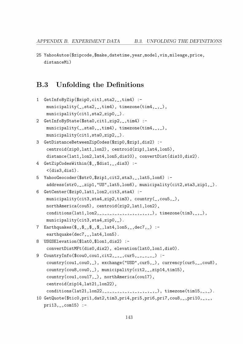
APPENDIX B. EXPERIMENT DATA B.3. UNFOLDING THE DEFINITIONS
25 YahooAutos($zipcode,$make,datetime,year,model,vin,mileage,price,
distanceMi)
B.3 Unfolding the Definitions
1 GetInfoByZip($zip0,cit1,sta2,_,tim4) :-
municipality(_,sta2,_,tim4), timezone(tim4,_,_),
municipality(cit1,sta2,zip0,_).
2 GetInfoByState($sta0,cit1,zip2,_,tim4) :-
municipality(_,sta0,_,tim4), timezone(tim4,_,_),
municipality(cit1,sta0,zip2,_).
3 GetDistanceBetweenZipCodes($zip0,$zip1,dis2) :-
centroid(zip0,lat1,lon2), centroid(zip1,lat4,lon5),
distance(lat1,lon2,lat4,lon5,dis10), convertDist(dis10,dis2).
4 GetZipCodesWithin($_,$dis1,_,dis3) :-
<(dis3,dis1).
5 YahooGeocoder($str0,$zip1,cit2,sta3,_,lat5,lon6) :-
address(str0,_,zip1,"US",lat5,lon6), municipality(cit2,sta3,zip1,_).
6 GetCenter($zip0,lat1,lon2,cit3,sta4) :-
municipality(cit3,sta4,zip2,tim3), country(_,cou5,_),
northAmerica(cou5), centroid(zip2,lat1,lon2),
conditions(lat1,lon2,_,_,_,_,_,_,_,_,_,_,_), timezone(tim3,_,_),
municipality(cit3,sta4,zip0,_).
7 Earthquakes($_,$_,$_,$_,lat4,lon5,_,dec7,_) :-
earthquake(dec7,_,lat4,lon5).
8 USGSElevation($lat0,$lon1,dis2) :-
convertDistMFt(dis0,dis2), elevation(lat0,lon1,dis0).
9 CountryInfo($cou0,cou1,cit2,_,_,cur5,_,_,_,_) :-
country(cou1,cou0,_), exchange("USD",cur5,_), currency(cur5,_,cou8),
country(cou8,cou0,_), municipality(cit2,_,zip14,tim15),
country(cou1,cou17,_), northAmerica(cou17),
centroid(zip14,lat21,lon22),
conditions(lat21,lon22,_,_,_,_,_,_,_,_,_,_,_), timezone(tim15,_,_).
10 GetQuote($tic0,pri1,dat2,tim3,pri4,pri5,pri6,pri7,cou8,_,pri10,_,_,
pri13,_,com15) :-
143

B.3. UNFOLDING THE DEFINITIONS APPENDIX B. EXPERIMENT DATA
trade(dat2,tim3,tic0,pri1), market(dat2,tic0,pri6,pri5,pri6,pri7,cou8),
sum(pri6,pri4,pri1), listing(_,com15,tic0,_), sum(pri5,pri13,pri10),
sum(pri4,pri10,pri1).
11 YahooExchangeRate($_,$cur1,pri2,dat3,_,pri5,pri6) :-
currentTime(tim0), time(tim0,_,_,dat3,_,_,_),
exchange("USD",cur1,pri2), currency(cur1,_,cou13),
country(cou13,cou15,_), exchange("USD",cur18,pri5),
currency(cur18,_,cou22), country(cou22,cou15,_), sum(pri2,pri5,pri28),
sum(pri2,pri6,pri28).
12 NOAAWeather($ica0,air1,_,_,sky4,tem5,hum6,dir7,spe8,_,pre10,tem11,_,_)
:- airport(ica0,_,air1,cit3,_,_,_,_), municipality(cit3,_,zip10,_),
country(_,cou13,_), northAmerica(cou13), centroid(zip10,lat17,lon18),
forecast(lat17,lon18,dat21,_,_,sky4,_,_,dir7,_,_),
time(_,_,_,dat21,_,_,_), municipality(cit3,_,zip39,tim40),
country(_,cou42,_), northAmerica(cou42), centroid(zip39,lat46,lon47),
conditions(lat46,lon47,_,tem5,sky4,tem11,hum6,_,spe8,_,pre58,_,_),
timezone(tim40,_,_), convertPress(pre58,pre10).
13 WunderGround($sta0,$cit1,tem2,_,_,pre5,pre6,sky7,dir8,spe9,spe10) :-
municipality(cit1,sta0,zip2,tim3), country(_,cou5,_),
northAmerica(cou5), centroid(zip2,lat9,lon10),
conditions(lat9,lon10,dat13,tem14,sky7,tem2,_,dir8,spe19,_,pre5,_,_),
timezone(tim3,_,_), municipality(cit1,sta0,zip29,_), country(_,cou32,_),
northAmerica(cou32), centroid(zip29,lat36,lon37),
forecast(lat36,lon37,dat40,tem41,_,_,_,_,_,spe10,_),
time(_,_,_,dat40,_,_,_), convertPress(pre5,pre6), <(tem14,tem41),
time(_,dat13,_,_,_,_,_), <(spe9,spe19).
14 WeatherBugLive($_,cit1,sta2,zip3,tem4,_,_,dir7,_,_) :-
municipality(cit1,sta2,zip2,tim3), country(_,cou5,_),
northAmerica(cou5), centroid(zip2,lat9,lon10),
conditions(lat9,lon10,_,tem4,_,_,_,dir7,_,_,_,_,_),
timezone(tim3,_,_), municipality(cit1,sta2,zip3,_).
15 WeatherFeed($cit0,$_,tem2,_,sky4,tem5,_,_,pre8,lat9,_,_) :-
municipality(cit0,_,zip2,tim3), country(_,cou5,_),
northAmerica(cou5), centroid(zip2,lat9,lon10),
conditions(lat9,lon10,_,_,sky4,tem5,_,dir18,_,_,pre8,_,_),
timezone(tim3,_,_), municipality(cit0,_,zip29,_), country(_,cou32,_),
144

APPENDIX B. EXPERIMENT DATA B.3. UNFOLDING THE DEFINITIONS
northAmerica(cou32), centroid(zip29,lat36,lon37),
forecast(lat36,lon37,dat40,_,tem2,_,_,_,dir18,_,_),
time(_,_,_,dat40,_,_,_).
16 WeatherByICAO($ica0,air1,cou2,lat3,lon4,_,dis6,_,sky8,_,_,_,_) :-
elevation(lat3,lon4,dis6), airport(ica0,_,air1,cit6,_,cou8,_,_),
municipality(cit6,_,zip13,_), country(cou8,cou16,_),
northAmerica(cou16), centroid(zip13,lat20,lon21),
forecast(lat20,lon21,dat24,_,_,sky8,_,_,_,_,_),
time(_,_,_,dat24,_,_,_), country(cou8,cou2,_).
17 WeatherByLatLon($_,$_,_,_,_,lat5,lon6,_,dis8,_,_,_,_,_,_) :-
elevation(lat5,lon6,dis8).
18 YahooWeather($zip0,cit1,sta2,_,lat4,lon5,day6,dat7,tem8,tem9,sky10) :-
municipality(cit1,sta2,zip2,_), country(_,cou5,_),
northAmerica(cou5), centroid(zip2,lat4,lon5),
forecast(lat4,lon5,dat7,tem9,tem8,sky10,_,_,_,_,_),
time(_,_,day6,dat7,_,_,_), municipality(cit1,sta2,zip0,_).
19 WeatherBugForecast($_,cit1,sta2,_,day4,sky5,tem6,_) :-
municipality(cit1,sta2,zip2,_), country(_,cou5,_),
northAmerica(cou5), centroid(zip2,lat9,lon10),
forecast(lat9,lon10,dat13,tem6,_,sky5,tim17,_,_,_,_),
time(_,_,day4,dat13,_,_,tim28), municipality(cit1,_,zip31,tim32),
country(_,cou34,_), northAmerica(cou34), centroid(zip31,lat38,lon39),
conditions(lat38,lon39,_,_,_,_,_,_,_,_,_,tim17,_),
timezone(tim32,tim28,_).
20 USFireHotelsByCity($cit0,_,_,sta3,zip4,cou5,_) :-
hotel(hot0,_,_,zip4,"US",_), hotelInfo(hot0,cou5),
municipality(cit0,sta3,zip4,_).
21 USFireHotelsByZip($zip0,_,_,cit3,sta4,cou5,_) :-
hotel(hot0,_,_,zip0,"US",_), hotelInfo(hot0,cou5),
municipality(cit3,sta4,zip0,_).
22 YahooHotel($zip0,$_,hot2,str3,cit4,sta5,_,_,_,_,_) :-
hotel(hot2,_,str3,zip0,"US",_), hotelInfo(hot2,_),
municipality(cit4,sta5,zip0,_).
23 GoogleBaseHotels($zip0,_,cit2,sta3,_,_,lat6,lon7,_) :-
municipality(cit2,sta3,zip2,tim3), country(_,cou5,_),
northAmerica(cou5), centroid(zip2,lat6,lon7),
145

B.3. UNFOLDING THE DEFINITIONS APPENDIX B. EXPERIMENT DATA
conditions(lat6,lon7,_,_,_,_,_,_,_,_,_,_,_),
timezone(tim3,_,_), municipality(cit2,sta3,zip0,_).
24 YahooTraffic($zip0,$_,_,lat3,lon4,_,_,_) :-
centroid(zip0,_,lon4), address(_,_,_,cou6,lat3,lon4),
country(cou6,_,_).
25 YahooAutos($zip0,$mak1,dat2,yea3,mod4,_,_,pri7,_) :-
car(mak1,mod4,_,yea3,vin4), car_details(vin4,_,zip0,_,_,pri7),
time(_,dat2,_,dat14,_,_,_), currentTime(tim18),
time(tim18,_,_,dat14,_,_,_).
146