1

Learning Sparse Codes for Hyperspectral ImageryAdam S. Charles, Bruno A. Olshausen, and Christopher J. Rozell

Abstract—The spectral features in hyperspectral im-agery (HSI) contain significant structure that, if properlycharacterized, could enable more efficient data acquisitionand improved data analysis. Because most pixels containreflectances of just a few materials, we propose that asparse coding model is well-matched to HSI data. Sparsitymodels consider each pixel as a combination of just afew elements from a larger dictionary, and this approachhas proven effective in a wide range of applications.Furthermore, previous work has shown that optimal sparsecoding dictionaries can be learned from a dataset withno other a priori information (in contrast to many HSI“endmember” discovery algorithms that assume the pres-ence of pure spectra or side information). We modified anexisting unsupervised learning approach and applied it toHSI data (with significant ground truth labeling) to learnan optimal sparse coding dictionary. Using this learneddictionary, we demonstrate three main findings: i) thesparse coding model learns spectral signatures of materialsin the scene and locally approximates nonlinear manifoldsfor individual materials, ii) this learned dictionary can beused to infer HSI-resolution data with very high accuracyfrom simulated imagery collected at multispectral-levelresolution, and iii) this learned dictionary improves theperformance of a supervised classification algorithm, bothin terms of the classifier complexity and generalizationfrom very small training sets.

Index Terms—Remote Sensing, Hyperspectral Imagery,Sparse Coding, Dictionary Learning, Multisepctral Im-agery, Deblurring, Inverse Problems, Material Classifica-tion

I. INTRODUCTION

Hyperspectral imagery (HSI) is a spectral imagingmodality that obtains environmental and geographicalinformation by imaging ground locations from airborneor spaceborne platforms. While multispectral imagery(MSI) acquires data over just a few (e.g., 3-10) irreg-ularly spaced spectral bands, HSI typically uses hun-

ASC and CJR are with the School of Electrical and ComputerEngineering at the Georgia Institute of Technology. BAO is with theHelen Wills Neuroscience Institute and School of Optometry at theUniversity of California, Berkeley. A preliminary version of portionsof this work appeared in [18]. The authors are grateful to CharlesBachmann at the Naval Research Laboratory for generously providingthe Smith Island HSI data set and the associated ground truth labels,as well as John Greer and Jack Culpepper for helpful discussionsabout this work.

dreds of contiguous bands that are regularly spacedfrom infrared to ultraviolet. For example, the WorldviewII MSI satellite [1] uses eight bands to represent thewavelengths from 0.435µm to 1.328µm, while typicalHSI has approximately 60 bands over the same rangein addition to many more bands at higher wavelengths.With spatial resolutions as low as 1m, the increasedspectral resolution of HSI means that estimated groundreflectance data can be used to determine propertiesof the scene, including material classification, geologicfeature identification, and environmental monitoring. Agood overview of HSI and the associated sensors can befound in [36].

Exploiting HSI is often difficult due to the particularchallenges of the remote sensing environment. For ex-ample, even “pure” pixels composed of a single materialwould have reflectance spectra that lie along a non-linear manifold due to variations in illumination, viewangle, material heterogeneity, scattering from the localscene geometry, and the presence of moisture [5], [36].Additionally, pure pixels are essentially impossible toactually observe due to material mixtures within a pixeland scattering from adjacent areas [36]. One of the mostcommon approaches to determining the material presentin a given pixel x (called “spectral unmixing” [37]) isto use a linear mixture model such as

x =

M∑k=1

φkak + ε, (1)

where {φk} is a dictionary of approximation elements,{ak} are the decomposition coefficients and ε is additivenoise. Note that {x,φk, ε} ∈ RN , where N is the num-ber of spectral bands and the vectors are indexed by λ(which is suppressed in our notation). When the dictio-nary represents spectral signatures of the various materialcomponents present in the scene, they are typically called“endmembers” and the resulting coefficients (assumedto sum to one) represent the material abundances ineach pixel. The endmember vectors are conceptualizedas forming a convex hull about the HSI data (e.g.,see the red vectors in Figure 1). Such a decompositionis often used for detecting the presence of a materialin the scene or classifying the materials present in apixel. A number of methods have been proposed for

2

determining endmembers, including algorithms whichselect endmembers from the data based on a measure ofpixel purity [48] or the quality of the resulting convexcone [53], tools that assist in the manual selection of end-members from the data [9], algorithms which optimizeendmembers for linear filtering [12], methods based onfinding convex cones using principal component anal-ysis (PCA) or independent component analysis (ICA)decompositions [21], [24], [27], [32], iterative statisticalmethods that optimize the resulting convex cone [10],and iterative measures to select optimal endmember setsfrom larger potential sets [50]. However, these algo-rithms either rely on postulating candidate endmembersets for initialization [50], assume the existence of purepixels in the scene [48], [53], attempt to encompassthe data within a cone rather than directly representthe data variations [9], [10], [32], use orthogonal linearfilters to attempt to separate out highly non-orthogonalspectra [12], or attempt to determine spectral statisticsfrom decompositions in the spatial dimensions ratherthan the spectral dimension. [21], [24]. None of thesemethods attempt to directly learn from the spectral dataa good representation of the low-dimensional, non-linearspectral variations inherent in HSI.

In addition to the difficulties determining the basicspectral components of an HSI dataset, there are manyresource costs (i.e., time, money, computation, avail-ability of sensor platforms) that result from the highdimensionally of the data. During data acquisition, thehigh resolution of HSI data comes at the expense ofsophisticated sensors that are costly and require rela-tively long scan times to get usable SNRs. After dataacquisition, it is evident that reducing the dimensionalitywhile retaining the exploitation value of the data wouldsave significant computational and storage resources. Ifthe higher-order statistics of the HSI data can be charac-terized, this information can be used to perform bothdimensionality reduction of existing high-dimensionaldata and high-resolution inference from low-resolutiondata (collected from either a cheaper MSI sensor ora modified HSI sensor measuring coarse spectral res-olution, thereby lowering scan times). One commonapproach to dimensionality reduction is PCA. However,the underlying Gaussian model in PCA means that it canonly capture pairwise correlations in the data and not thehigher-order (and non-Gaussian) statistics present in HSIdata.

Following on developments in the computational neu-roscience community, the signal processing communityhas recently employed signal models based on thenotion of sparsity to characterize high-order statisticaldependencies in data and yield state-of-the-art results

in many signal and image processing algorithms [20].Specifically, this approach models a noisy measurementvector x as being generated by a linear combination ofjust a few elements from the dictionary {φk}. This isthe same model as in (1), but where the coefficients arecalculated to have as few non-zero elements as possible.Much like PCA, sparse coding can be viewed as a typeof dimensionality reduction where a high dimensionaldataset is expressed in a lower dimensional space ofactive coefficients. However, while PCA calculates justa few principal components and uses essentially allof them to represent each pixel, sparse coding modelstypically employ a larger dictionary but use only a fewof these elements to represent each pixel. When cast interms of a probabilistic model, this sparsity constraintcorresponds to a non-Gaussian prior that enables themodel to capture higher order statistics in the data.

Due to the high spatial resolution of modern HSIsensors (resulting in just a few dominant materials in apixel), sparsity models seem especially relevant for thissensing modality. In fact, initial research into sparsitymodels for spectral unmixing in HSI has shown promis-ing results [29], [33]. While a sparse decomposition canbe estimated for any dictionary, previous research [43]has shown that unsupervised learning techniques canbe used in conjunction with an example dataset toiteratively learn a dictionary that admits optimally sparsecoefficients (without requiring the dataset to contain any“pure” signals that correspond to a single dictionaryelement). These methods leverage the specific high-orderstatistics of the example dataset to find the underlyinglow-dimensional structure that is most efficient at repre-senting the data.

In contrast to the typical endmember model describedabove, the sparse coding model does not assume that thedata lie within the convex hull of the dictionary. Instead,the learned sparse coding dictionary elements will tendto look like the basic spectral signatures comprisingthe scene (early encouraging evidence of this can befound in [28]). In fact, the sparse coding model mayactually learn several dictionary elements to representsome types of materials, especially when that materialspectra demonstrates highly nonlinear variations withinthe scene. Because of the sparsity constraint, one wouldexpect these learned dictionaries to reflect the specificstatistics of the HSI data by locally approximating thesenonlinear data manifolds [45] (as illustrated in Figure 1,and in contrast to typical endmember models that forma convex hull containing the data).

We have modified the unsupervised learning approachdescribed in [43] and applied it to HSI data to learn a

3

Fig. 1. Typical endmember analysis uses vectors that composea convex hull around the data. In this stylized illustration, thedata manifold is indicated by the dashed line and the red vectorsrepresent the endmembers. In contrast, a learned dictionary for sparsecoding attempts to learn a local approximation of the nonlinear datacharacteristics directly (indicated here by blue vectors).

dictionary that is optimized for sparse coding. Impor-tantly, the HSI dataset used in this study has signifi-cant ground truth labeling of material classes makingit possible to examine the characteristics of the learneddictionary relative to the data. Using this learned dic-tionary, we make three main contributions. First, weshow that the sparse coding model learns meaningfuldictionaries that correspond to known spectral signatures:they locally approximate nonlinear data manifolds forindividual materials, and they convey information aboutenvironmental properties such as moisture content ina region. Second, we generate simulated imagery atMSI-level resolution and show that the learned HSIdictionaries and sparse coding model can be effectivelyused to infer HSI-resolution data with very high accuracy(even for data of the same region collected in a differentseason). Finally, we use ground truth labels for the HSIdata to demonstrate that a sparse coding representationimproves the performance of a supervised classificationalgorithm, both in terms of the classifier complexity (i.e.,classification time) and the ability of the classifier togeneralize from very small training sets.

II. BACKGROUND AND RELATED WORK

A. Methods

Given a pixel x ∈ RN and a fixed dictionary {φk}with φk ∈ RN for k ∈ [1, . . . ,M ], the goal of sparsecoding is to find a set of coefficients that represent the

data well using as few non-zero elements as possible.Written mathematically, the goal is to minimize anobjective function that combines data fidelity and asparsity-inducing penalty. A common choice is to usea regularized least-squares objective function such as,

Jγ (x, {ak}, {φk}) =

∥∥∥∥∥x−M∑k=1

φkak

∥∥∥∥∥2

2

+ γ

M∑k=1

|ak|,

(2)

with mean-squared error as the data-fidelity term, the`1 norm (i.e., the sum of the coefficient magnitudes)as the sparsity inducing penalty, and γ a scalar pa-rameter trading off between these two terms [19].This objective is convex in the coefficients when thedictionary is fixed, meaning that solving {ak} =arg min{ak} Jγ (x, {ak}, {φk}) is a tractable optimiza-tion. Significant progress has recently been made de-veloping solvers that are customized for this specificoptimization program and run considerably faster thangeneral purpose algorithms [15], [22], [30], [38]. Thisgeneral approach is applicable directly to HSI withone small modification: we constrain the coefficientsto be non-negative (ak ≥ 0) to maintain physicalcorrespondence between the coefficients and the relativeabundance of material spectra present in the scene. Dueto its wide use in the community, its ability to enforcepositive coefficients without a sum-to-one constraint, andestablished reputation for quick convergence, we use thespecialized optimization package described in [38] tosolve this constrained optimization and calculate sparsecoefficients. While other solvers have been explored inthe specific context of HSI [11], [46] that may be fasterin some settings, many of these HSI-specific solversinclude additional constraints which we do not employ(e.g.

∑k |ak| = 1). The framework we present here is

largely agnostic to the specific solver as long as it returnsaccurate solutions, so other choices could be substitutedif there were advantages for a given application. Adetailed analysis of various algorithms to optimize (2)in the context of HSI unmixing is given in [33].

An alternate interpretation of the cost function in (2)is to consider the problem as Bayesian inference. With awhite Gaussian noise distribution on ε, the likelihood onthe data vector given the coefficients p(x|{ak}) is alsoGaussian. We assume a Laplacian prior probability distri-bution on the coefficients {ak} because the high kurtosisof this distribution (i.e., the peakiness of the distributionaround zero) encourages coefficients to be close to zero.Using Bayes’ rule, the resulting (unnormalized) posterior

4

is

p({ak}|x) ∝ p(x|{ak})p({ak})

∝ e(− 1

2σ2ε‖x−

∑k φkak‖22

)e

(−

√2

σa

∑k |ak|

),

where σa is the standard deviation on the prior over ak(i.e., the signal energy) and σ2ε is the noise variance.Taking the negative logarithm of the posterior resultsin the cost function (2). Thus the maximum a poste-riori (MAP) estimate on the coefficients is equivalentto minimizing (2) with γ = 2

√2σ2ε /σa. This Bayesian

formulation allows us to naturally extend the sparseapproximation problem to more general observationmodels and inverse problems, such as the high resolutioninference task described in Section III-B and similarinverse problems described in [55]. Note also that thesparse prior introduces a non-Gaussianity into the modelthat is critical for capturing the high-order data statistics.An approach such as PCA that fundamentally assumesa Gaussian data model can only learn from pairwisecorrelations in the data, and is therefore unable to capturethe higher-order statistics.

To learn an optimal dictionary for sparse cod-ing, we would like to minimize the cost functionJγ (x, {ak}, {φk}) with respect to both the coefficientsand the dictionary. Unfortunately, this objective func-tion is not jointly convex in the coefficients and thedictionary, making global minimization prohibitive. Thework presented in [43], [44] takes a typical approachto this type of problem, using a variational method thatalternates between minimizing (2) with respect to thecoefficients given the current dictionary, then taking agradient descent step over the dictionary elements giventhe calculated coefficients. Specifically, after inferringcoefficients for a randomly selected batch of data, thedictionary learning proceeds by descending the gradientof Jγ (x, {ak}, {φk}) with respect to {φk}, resulting inthe learning rule:

φl ← φl + µ

⟨al

(x−

M∑k=1

φkak

)⟩, (3)

where µ is the step-size of the update (possibly varyingwith iteration number) and 〈·〉 indicates the average overthe current batch of data. This approach has the drawbackthat a trivial solution of enlarging the norm of the dictio-nary elements can always produce smaller total energyin the coefficients, which we avoid by renormalizing thedictionary elements to have unit norm after each learningstep. Returning briefly to the Bayesian interpretationdetailed above, it is worth noting that the cost functionJγ (x, {ak}, {φk}) may be viewed as an approximation

to the negative log-likelihood of the model [44]. There-fore, gradient descent on Jγ (x, {ak}, {φk}) is tanta-mount to maximizing the log-likelihood of the model.As with the coefficient optimization, other algorithmshave been proposed for the learning step that couldbe substituted for this steepest decent approach. Inparticular, many other methods (including the recentlyproposed K-SVD) use second order information in thelearning step to reduce the number of learning iterationsrequired for convergence (though this may come at thecost of increasing the batch size per iteration to get betterestimates for the update step) [2], [3].

The results in [43], [44] demonstrate that this unsu-pervised approach can start with an unstructured randomdictionary and recover known sparse structure in simu-lated datasets, as well as uncover unknown sparse struc-ture in complex signal families such as natural images.We again adopt this general approach with a small mod-ification: we constrain the dictionary elements to be non-negative (φk ≥ 0) to maintain physical correspondencewith spectral reflectances. To be concrete, the dictionarylearning method we use is specified in Algorithm 1,and we determine convergence visually by when thedictionary elements stopped adapting. In our experience,most of the dictionary elements were well-convergedby 1000 iterations of the learning step (approximately50 minutes of computation on an 8-core Intel XeonE5420 with 14GB of DDR3 RAM). Some dictionaryelements corresponding to less prominent materials (thatare randomly selected less often during learning) seemto require 10,000-20,000 learning iterations to converge(approximately 10-15 hours on the same machine). Weoften conservatively let the algorithm run for 20,000to 80,000 iterations at a smaller step size to assuregood convergence. The increasing prevalence of parallelarchitectures in multi-core CPUs and graphics processingunits should provide increasing opportunities to speed upthis type of unsupervised learning approach.

Finally, we note that the proposed approach can havelocal minima or non-unique solutions in at least tworespects, especially in the case of HSI. First, thoughthe coefficient optimization using an `1 sparsity penaltyis convex, the ideal `0 sparse solution may not beunique when the one-sided coherence of the dictionarymaxi 6=j |〈φi,φj〉|/‖φi‖22 is large [13]. Second, thoughthere are few analytic guarantees about the performanceof dictionary learning algorithms, recent results indicatethat the ideal dictionary is more likely to be a localsolution to the optimization presented here when thecoherence of the dictionary is also low [26]. Since manymaterials have spectral signatures with high correlation

5

Algorithm 1 Sparse coding dictionary learning algo-rithm of [44], modified for HSI.

Set γ = 0.01Set µ = 10Initialize {φk} to random positive valuesrepeat

for i = 1 to 200 doChoose HSI pixel x uniformly at random{ak} = arg min J ({ak}, {φk}) s.t. ak ≥ 0

∆φl(i) = al

(x−

∑Mk=1φkak

)end forφl ←

[φl + µ

200

∑i ∆φl(i)

]+

µ← 0.995µuntil {φk} converges

in some bands, typical HSI dictionary databases have co-herence values very close to unity [33], and we observesimilar values in our learned dictionaries. Despite notbeing favorable for the technical results described aboveregarding coefficient inference and dictionary learning,the inferred coefficients and learned dictionaries appearto be robust and useful in the applications describedhere. Indeed, it is likely in these cases that despitethere being many local solutions (and a unique minimaperhaps even not existing), many of the suboptimalsolutions are also quite good and useful in applications.In particular, we have repeated the dictionary learningexperiments described in this paper many times (withdifferent random initial conditions), with no significantchanges in the qualitative nature of the dictionary orthe performance in the tasks highlighted in Section III.This also corresponds to the results in [33] showing thatdespite the near-unity coherence in a standard hyperspec-tral endmember dictionary, these dictionaries can yieldgood sparse representations useful in spectral unmixingapplications.

B. Hyperspectral dataset and learned dictionaries

In this paper we apply the dictionary learning methoddescribed in Algorithm 1 to learn a 44-element dictionaryfor a HSI scene of Smith Island, VA. This scene has 113usable spectral bands (ranging from 0.44–2.486µm) ac-quired by the PROBE2 sensor on October 18, 2001.1 Thedata has a spatial resolution of approximately 4.5m andwas postprocessed to estimate the ground reflectance. Ofthe 490,000 pixels in the dataset, 2700 pixels are tagged

1Smith Island is a barrier island that is part of the Virginia CoastReserve Long-Term Ecological Research Project. For more details,see http://www.vcrlter.virginia.edu. This dataset was generously pro-vided by Charles Bachmann at the Naval Research Laboratory.

with ground truth labels drawn from 22 categories. Thesecategories include specific plant species and vegetationcommunities common to wetlands, and were determinedby in situ observations made with differential GPSaided field studies during October 8–12, 2001. Moreinformation about the HSI dataset and the ground truthlabels can be found in [4], [6]–[8]. The size of thedictionary (44 elements) was made to ensure that therewere multiple elements available for each of the 22known material classes in this particular dataset. Thenumber 44 represented a compromise between smallerdictionaries that didn’t perform as well on the tasksdescribed in Section III (especially the local manifoldapproximation), and larger dictionaries that presentedmore difficulty getting all of the elements to convergein the learning.2 In general, determining the optimalnumber of dictionary elements to learn for a dataset isan open question and could be a valuable future researchdirection.

We cross-validated the results of this paper in twoways. First, 10,000 randomly selected pixels were ex-cluded from the dataset before the dictionary learningso that they could be used in testing. Second, we alsohave available data from another HSI collection of thesame geographic region using the same sensor on August22, 2001. While this is close enough in time to assumethat there are no major geologic changes in the scene,this data does come from a different season where thevegetation and atmospheric characteristics are potentiallydifferent, resulting in different statistics from the dataused in the learning process. We use this dataset specifi-cally to assess the potential negative effects of mismatchbetween the statistics of the training and testing datasetswhen performing signal processing applications usingthe learned dictionary.

C. Related work

Prior work in using unsupervised methods to learnHSI material spectra has used some algorithms that arevery related to our present approach. For example, ICAcan be viewed as finding linear filters that give highsparsity, and prior work [23], [27], [51] demonstrates thatICA can be effective at determining a range of spectralsignatures from preprocessed data. Other approachesalso based on Bayesian inference (but not necessarilya sparsity-inducing prior) [41] have been used to learn

2While performance in the signal processing tasks we tested didimprove with larger dictionaries, we note that the performance differ-ence was often relatively minor when using 22 element dictionariesand this size would likely be sufficiently for this dataset in manyapplications.

6

HSI dictionaries, but this approach has trouble includinginformation from large datasets and often uses ICA asa preprocessing stage to reduce the number of pixelsto analyze. The technique most closely related to ourcurrent approach is blind source separation based on non-negative matrix factorization (NMF) [35], [47]. Whilenot explicitly incorporating sparsity constraints, resultsusing NMF have been shown to exhibit sparse behav-ior [31]. In the NMF setup, the sparsity level of thedecomposition is difficult to control [31] and previouswork in [35] mitigates this by adding an explicit sparsityinducing term. Additionally, the above mentioned ap-proaches all retain the sum-to-one constraint, which wedrop due to the variable power in the pixels throughoutthe scene.

In addition to these results on unsupervised learning,as well as additional encouraging prior work on usingsparsity models for spectral unmixing [29], [33] andlearning dictionaries that resemble material spectra [28],Castrodad et al. [16] have explored using a sparsitymodel and learned dictionaries to improve supervisedclassification performance on HSI data.3 In Section III-Cwe will explore the advantages of using sparse coef-ficients from a learned dictionary in an off-the-shelfclassification algorithm. In [16], the authors use labeleddata to learn a separate dictionary for each class andclassify data by determining which of these candidatedictionaries best describes an unknown pixel (definedby having the minimum value for the objective functionin equation (2)). This approach is customized to theclassification problem, and we expect the classificationperformance would outperform the general approachwe describe in Section III-C. In contrast, the approachin [16] requires a more computationally expensive learn-ing process (due to the multiple dictionaries), requireslabeled data before the learning process, and generatesa dictionary that is tailored to the classification task andmay not generalize as well to other tasks.

Zhou et al. [55] have explored using a sparsity modeland learned dictionaries to effectively solve inverseproblems in HSI. In Section III-B we will explore theability of sparse coefficients from a learned dictionary toinfer high resolution spectral data from low resolutionimagery by formulating the task as a linear inverseproblem. In [55], the authors show that when removingsubstantial amounts of data from an HSI datacube, alearned dictionary can be used to exploit the correlationstructure present in each band to infer the missing data

3The authors in [16] use a different learning algorithm (K-SVD [2])from our gradient approach, but it is attempting to achieve the samegoal of learning an optimal dictionary for sparse approximation.

and reconstruct the spatial image associated with eachband. This inpainting task is a very similar inverseproblem to the one we examine in Section III-B, differingprimarily in the type of measurement operator used in themodel (i.e., blurring vs. subsampling) and the dimensionof the data used in the learning and reconstruction (i.e.,spectral vs. spatial).

III. MAIN RESULTS

A. Learned Dictionary Functions

While the learning procedure described in Algorithm 1adapts the dictionary to the high-order statistics of theHSI data, there are no constraints added that ensure theresulting dictionary elements will correspond to physicalspectra or be informative about material properties inthe scene. To examine the properties of the learneddictionary, examples elements are plotted in Figure 2.It is clear that these dictionary elements not only havethe general appearance of spectral reflectances, they alsomatch the spectral signatures of many of the materialsthat are known to be in the scene. Using the ground truthlabels from the Smith Island dataset (which denote thedominant material present in the pixel), Figure 2 showsan example spectral signature from a class along withthe dictionary element that has the largest coefficient inthe sparse decomposition of that pixel. Despite beinggiven no a priori information about the data beyondthe sparsity model (i.e., without being given the classlabels and corresponding pixels), the algorithm learnsspectral shapes that correspond to a number of compo-nent material spectra present in the image. These learneddictionaries cover a wide variety of distinct materialclasses for which we have ground truth labels, including“Pine”, “Water”, “Mud” and “Distichlis”, as well as verysimilar spectra, such as “Water” and “Submerged Net”or “Pine trees” and “Iva”.

In contrast, Figure 3 shows the first four principalcomponents found through PCA analysis on the sameHSI dataset, which is sufficient to capture 99.9% of thevariance in the data. While the first principal componentdoes have some similarity to a general vegetation spec-trum, the other spectral components do not correspondto physically meaningful spectral features. Figure 3 alsoshows the comparison between the decomposition coeffi-cient in the sparsity model and PCA for all pixels in fourof the labeled classes. The raster plots show that whilethe sparse decomposition and the principal componentsboth only need a few coefficients to represent the data,the sparse decomposition chooses different coefficientsfor different spectral shapes (i.e., the material informa-tion is encoded in the selection of active coefficients)

7

Fig. 2. Example spectra for materials in the labeled classes of the Smith Island dataset and the learned dictionary element (DE) that is theclosest match for each example. The two obvious gaps in the spectra are bands removed from consideration in the original dataset due tothe interactions with the atmosphere in these regions.

Fig. 3. (Left) The top four principal components for the Smith Island dataset (capturing 99.9% of the variance). In contrast to the learneddictionary elements in Figure 2, only one of the principle components looks generally like a spectral signature. (Right) PCA and sparse codingcoefficients representing every sample of the data from three of the labeled classes (“Andropogon”, “Sand”, and “Submerged Net”). Thebrightness at each pixel represents the intensity of a given coefficient for a specific pixel. Note that PCA uses many of the same coefficientsfor different materials (e.g., coefficient 1 is always used), while sparse coding tends to select distinct coefficients for the different materials.

whereas PCA uses the same four vectors to representnearly all of the data. This comparison illustrates thatthe learned dictionary under the sparsity model has amuch closer correspondence to the individual spectralcharacteristics found in the dataset than PCA, indicatingthat this representation may have many advantages fortasks such as classification.

While it is clear that the dictionary elements arelearning spectral elements present in the scene, thisrepresentation will be most meaningful if there is consis-tency in the way environmental features are represented.In other words, when looking across the scene, do thesparse decompositions change in a way that reflectsthe changes in the underlying geologic features? We

8

Fig. 4. Progression of sparse coding coefficients from a row of contiguous pixels in the Smith Island dataset. (Upper left) The red lineindicates a row of 300 pixels selected for analysis. These pixels (numbered left to right) represent a progression from an inland region to thewater off the east coast of the island. (Upper right) The sparse coding coefficients for the row of pixels is shown, where the brightness of apixel indicates the intensity of each coefficient for each pixel. Note that many of the same coefficients are often active in the same geographicregions, and the progression from one type of element to another (e.g., sand to water) can be seen by different coefficients dominating thedecomposition. (Bottom) The spectra for pixels 1, 25, 50, 75, 100, 150, 200 and 300 are shown in the bottom row (in black), along withthe two most active dictionary elements in the top two rows (color coded). The fractional abundance for each dictionary element in eachpixel is given by r = |ai|/‖a‖1. Note that many of the same dictionary elements can be seen dominating the decomposition in regions withsimilar material composition.

extracted a row of pixels from the Smith Island dataset,starting inland and ending in the water off the coastof the island. The selected row of pixels is shown inred in Figure 4, superimposed on a magnified RGBrendering of that portion of the island. Figure 4 shows thecoefficient decomposition of each pixel, as well as themeasured spectrum and the two most active dictionaryelements at various locations along the row. Includedwith each of the two most active dictionary elements isthe fractional abundance r = |ai|/‖a‖1 of that dictionaryelement in the decomposition. This row starts withmostly vegetation spectra for the first 75 pixels, changingto sand-like spectra by the the 100th pixel and eventuallyto water spectra by the 160th pixel.

We highlight two important properties of the coeffi-cient decompositions over the pixel progression in theraster plot in Figure 4. First, the sparse coefficients arerelatively consistent over contiguous spatial ranges, with

the same small sets of coefficients generally dominat-ing the decomposition over small contiguous regions.While this is evident in the regions dominated by sandand water, there are also repeated dictionary elementsacross several spatial locations in the regions dominatedby vegetation (which we would expect to have muchmore variability over pixels with 4m resolution). Second,some slowly changing geologic properties are actuallyobservable in the gradual onset and offset of specificdictionary elements in the decomposition. One prominentexample of this is the slow change from dictionaryelement 8 to dictionary element 44 over the span ofwater moving away from the shoreline, indicating theslow fading of shallow water to deep water (which havedifferent spectral characteristics and are represented bydifferent dictionary elements). Another example of thisis the rise of dictionary element 9 from the second mostactive to the most active element from pixels 75 and 100,

9

indicating the slowly increasing presence of a particularvegetation characteristic in this region.

In addition to the spectral matches shown in Figure 2and the spatial coefficient variations shown in Figure 4,another important aspect of the learned dictionary is toexamine how it represents the nonlinear variations withina particular material class [5]. For example, Figure 5shows full spectral signatures for a patch of water offthe coast of Smith Island, as well as spectral bands 14,29 and 70 (0.6278, 0.8572 and 1.4962 µm) from threedifferent view angles to show the geometry of thesepoints in 3-D spectral space.4 Despite being one materialclass (“water”), it is evident even in these few bandsthat the measured spectrum lies on a nonlinear manifold.Superimposed on the 3-D spectral plots are five of thelearned dictionary elements projected onto these samethree spectral bands. The measured spectra are colorcoded to indicate which of these five learned dictionaryelements are dominant in their sparse decomposition.The contiguity of this color coding over small manifoldregions demonstrates that rather than containing the mea-sured spectra in a convex hull, the learned dictionariesare essentially forming a local linear approximation tothis manifold. So, despite being a linear data model,the dictionary learns multiple elements that capture thenonlinear spectral variations by locally approximatingthe manifold structure in a meaningful way. In ourexperiments with other endmember extraction algorithmssuch as [53], the learned sparse dictionary does appearto produce a representation that more closely tracks thenonlinear variations in the data points (e.g., produces asmaller relative MSE between the data and the dictionaryelements) compared to a method restricted to finding aconvex cone around the data. A more detailed character-ization of the differences between various linear modelsat representing nonlinear material variations would be avaluable direction for future research.

B. Reconstructing HSI-resolution from MSI-resolutiondata

As discussed earlier, while the high spectral resolutionof HSI is valuable, acquiring data at this resolutioncomes at a cost. In terrestrial remote sensing, hyperspec-tral imagers are relatively rare instruments, and it wouldbe much more resource efficient to perform most spectralimaging at MSI-level resolution. Data at this resolutioncould either be gathered by actual MSI sensors, or byHSI sensors modified to decrease their spectral resolu-tion (which could potentially decrease scan times). The

4These are the same spectral bands and approximately the sameregion highlighted in Figure 1 of [5].

question we consider here is whether a dictionary learnedon an HSI training set could be used to accurately inferhigh resolution spectra from subsequent data collectedat MSI-level spectral resolution.

In this basic paradigm, assume that we start with alearned dictionary that has been adapted to the specificstructure of the desired HSI data. This could arise fromearlier HSI of the scene being imaged, or imaging fromother geographic regions with similar environmentalfeatures (and therefore similar statistics). For the newdata acquired at MSI-level resolution, we assume for afirst approximation that each band is a linear combinationof some group of spectral bands in the underlying trueHSI data. Specifically, we model the MSI-resolution dataas

y = Bx+ ε = B

M∑k=1

φkak + ε, (4)

where y ∈ RL (L < N) is the new coarse resolution dataand B can be thought of as an (L×N) “blurring” matrixthat bins the spectral bands of the desired HSI data.While B could be any matrix describing the sensitivityfunction of the imager acquiring the MSI-resolution data,we will consider B that simply sums spectral bands overa contiguous range.

This measurement paradigm fits nicely into the well-known framework of Bayesian inference (or equivalently,linear inverse problems in image processing). Essentially,given the wealth of information about the statistics ofthe HSI we would like to obtain, Bayesian inferenceallows one to optimally answer the question of whatunderlying HSI data x is most likely given the observedMSI-resolution data y. Specifically, given the new modelin (4), the likelihood of the data y given the coefficients{ak} is now the Gaussian distribution

p(y|{ak}) ∝ e− 1

2σ2ε‖y−B

∑k φkak‖22 .

We can again use an independent Laplacian prior onthe sparse coefficients {ak}, and write the posteriordistribution using exactly the same simplifications asbefore. The optimal MAP estimate of the sparse coef-ficients given the observed data y is therefore given byoptimizing the following objective function with respectto the coefficients:

Jγ (y, {ak}, {φk}) =

∥∥∥∥∥y −BM∑k=1

φkak

∥∥∥∥∥2

2

+ γ∑k

|ak|.

(5)

This optimization program is very similar to (2) (and canbe solved by the same software packages), but incorpo-

10

Fig. 5. The nonlinear structure of water pixels is locally approximated by the learned dictionary. The plots in the upper left, upper rightand bottom right all show the spectra water pixels (selected from a contiguous region) projected onto three spectral bands (14,29,70). Evenin three dimensions, it is clear that the data live on a nonlinear manifold, and there is clear structure in the variability. The vectors representthe projection onto the same three bands of five learned dictionary elements. The points representing water pixels are color coded to indicatewhich dictionary element has the largest value when inferring the sparse coefficients, showing that contiguous values on the manifold arecoded using the same dictionary element.

Fig. 6. Reconstructing spectra with HSI resolution from measurements with MSI-level resolution. (Top) A schematic of the process forsimulating low resolution spectral data and performing recovery. The matrix B characterizes the measurement process (i.e., the sensitivityfunction of the sensor), simulating the aggregation of high resolution spectral information into low resolution spectral bands. (Bottom left)A diagram indicating the sensitivity function for MSI resolution measurements, where 113 HSI bands are collapsed into 8 equally spacedmeasurement bands over the lowest wavelengths (approximately matching the spectral bands reported by the Worldview II MSI sensor). Notethat no information is measured from the highest wavelength regions. (Bottom right) A diagram indicating the sensitivity function for coarseHSI measurements, where 113 HSI bands are collapsed into 8 nearly equally spaced measurement bands across the whole HSI spectrum.

rates the measurement process described by B into theinference. Given the estimated sparse coefficients, theHSI vector x is reconstructed according to (1): x =∑

k φkak. The full workflow is shown schematically inFigure 6. We note that many linear inverse problems are

formulated in a similar way depending on the choiceof B, including inpainting missing data such as theapplication considered by [55].

For proof-of-concept simulations we generated sim-ulated data with MSI-level resolution from pixels thatwere not used in the training dataset, and perform

11

TABLE IRELATIVE RECOVERY ERROR FOR HSI SPECTRA FROM COARSE HSI MEASUREMENTS (FULL SPECTRUM). RESULTS ARE REPORTED FORTESTING DATA COLLECTED ON THE SAME DAY (SD) AS THE TRAINING DATA USED TO LEARN THE DICTIONARY, AS WELL AS RESULTS

FOR TESTING DATA COLLECTED ON A DIFFERENT DAY (DD).

Mean Error (SD) Median Error (SD) Mean Error (DD) Median Error (DD)44 Learned DE 8.249x10−4 4.911x10−4 7.054x10−3 6.005x10−3

44 Exemplar DE 6.280x10−3 2.709x10−3 1.493x10−2 1.105x10−2

44 Random DE 4.143x10−1 4.524x10−1 3.965x10−1 4.165x10−1

TABLE IIRELATIVE RECOVERY ERROR FOR HSI SPECTRA FROM MSI MEASUREMENTS (NO MEASUREMENTS FROM HIGHEST WAVELENGTHS).

RESULTS ARE REPORTED FOR TESTING DATA COLLECTED ON THE SAME DAY (SD) AS THE TRAINING DATA USED TO LEARN THEDICTIONARY, AS WELL AS RESULTS FOR TESTING DATA COLLECTED ON A DIFFERENT DAY (DD).

Mean Error (SD) Median Error (SD) Mean Error (DD) Median Error (DD)44 Learned DE 1.271x10−2 1.791x10−3 2.456x10−2 1.219x10−2

44 Exemplar DE 1.132x10−2 5.552x10−3 2.225x10−2 2.135x10−2

44 Random DE 7.845x10−1 8.974x10−1 7.775x10−1 9.946x10−1

the inference process described above to estimate thehigh-resolution spectra from the low-resolution measure-ments. In the first set of simulations, the matrix B(illustrated in Figure 6) generates simulated data with 8equally spaced bands covering the entire spectral rangeof the HSI data. This B is intended to model a hyper-spectral imager collecting spectral data with an orderof magnitude less spectral resolution than the originaldata. We used two testing datasets in this simulation:the 10,000 pixels from the October 2001 scan of SmithIsland that were withheld from the learning process,and 10,000 randomly selected pixels from the August2001 scan of the same geographic region. By using HSIcollected on a different date we can examine the effectsof using a dictionary that was learned on data with dif-ferent statistics than the data we are trying to reconstruct(due to different vegetation characteristics in the differentseasons and different atmospheric conditions present onthe different days).

We infer the sparse coefficients in the HSI dictionarygiven the simulated MSI-resolution data by minimizingthe objective function in Equation (5) as described above.For comparison purposes and to determine the value ofthe learning process in the reconstruction, we repeatedthis recovery process with a 44-element dictionary ofrandom values (i.e., the initialization conditions for thedictionary learning) and with an exemplar dictionaryformed by taking two random spectral signatures fromeach class in the original labeled HSI data (for a total of44 dictionary elements). Figures 7 and 8 show examplesof the original HSI, the simulated coarse resolutiondata, the estimated sparsity coefficients in the learneddictionary, and the subsequent recovered HSI data for

the test datasets collected on the same date (SD) and adifferent date (DD) as the training dataset. The set ofexamples shown in the figure span the range of the mostfavorable and least favorable reconstructions.

Table I reports the average relative MSE for thereconstructions, calculated as

ei =‖xi − xi‖22‖xi‖22

. (6)

The aggregate results as well as the specific plottedexamples demonstrate that the HSI-resolution data isrecovered with less than 0.09% relative MSE for theSD testing set and less than 0.71% relative MSE onthe DD testing set. While the reconstruction is worse onthe DD dataset because of the mismatch in the trainingand testing statistics, the reconstructions are still verygood overall and often capture even fine detail in theHSI spectra. Also note that the learned dictionary isperforming significantly better than both the exemplardictionary (which was chosen using oracle knowledgeof the classes to ensure good coverage of the variousmaterials) and the random dictionary (indicating thevalue of the learning process).

In the second set of simulations, the matrix B (il-lustrated in Figure 6) generates simulated data with 8equally spaced bands excluding the highest wavelengthregions. This B is intended to model a multispectral im-ager, and we selected the bands to approximately matchthe reported bands of the WorldView II multispectralsensor. We used the same SD and DD testing datasets inthe simulation, with Figures 9 and 10 showing examplereconstructions and Table II reporting average recon-struction results. While the overall performance does

12

Fig. 7. Reconstructing HSI data from simulated coarse HSI measurements using training and testing data collected on the same date. Plotsshow original HSI spectrum in blue (113 bands), simulated coarse HSI spectrum (8 bands), inferred sparse coefficients, and reconstructedHSI spectrum in green. Examples were selected to illustrate a range of recovery performance, from examples of the best recovery on top toexamples of the worst recovery on the bottom.

Fig. 8. Reconstructing HSI data from simulated coarse HSI measurements using training and testing data collected on different dates(in different seasons). Plots show original HSI spectrum in blue (113 bands), simulated coarse HSI spectrum (8 bands), inferred sparsecoefficients, and reconstructed HSI spectrum in green. Examples were selected to illustrate a range of recovery performance, from examplesof the best recovery on top to examples of the worst recovery on the bottom.

13

Fig. 9. Reconstructing HSI data from simulated MSI measurements using training and testing data collected on the same date. Plots showoriginal HSI spectrum in blue (113 bands), simulated coarse HSI spectrum (8 bands), inferred sparse coefficients, and reconstructed HSIspectrum in green. Examples were selected to illustrate a range of recovery performance, from examples of the best recovery on top toexamples of the worst recovery on the bottom.

suffer compared to the previous experiment when thewhole spectral range was measured, the HSI spectra areagain recovered with low error overall: less than 1.28%for the SD dataset, and less than 2.47% error for theDD dataset. As expected from the previous simulation,the lower wavelengths can be reconstructed very well.As might be expected because no data was collectedin the higher wavelength range, the recovery in thesespectral bands can suffer from higher errors even despitegetting the general shape correct. Table II also showsthat overall, both the learned and exemplar dictionarieshave approximately the same mean relative error in thissetting. However, the distribution of the relative errorsover the test pixels is more tightly peaked about theorigin for the learned dictionary, with a median relativeerror approximately a third of that for the exemplardictionary. This indicates that while most test pixels wererecovered better with the learned dictionary, there werea minority of pixels that suffered more egregious errorsthan seen with the exemplar dictionary.

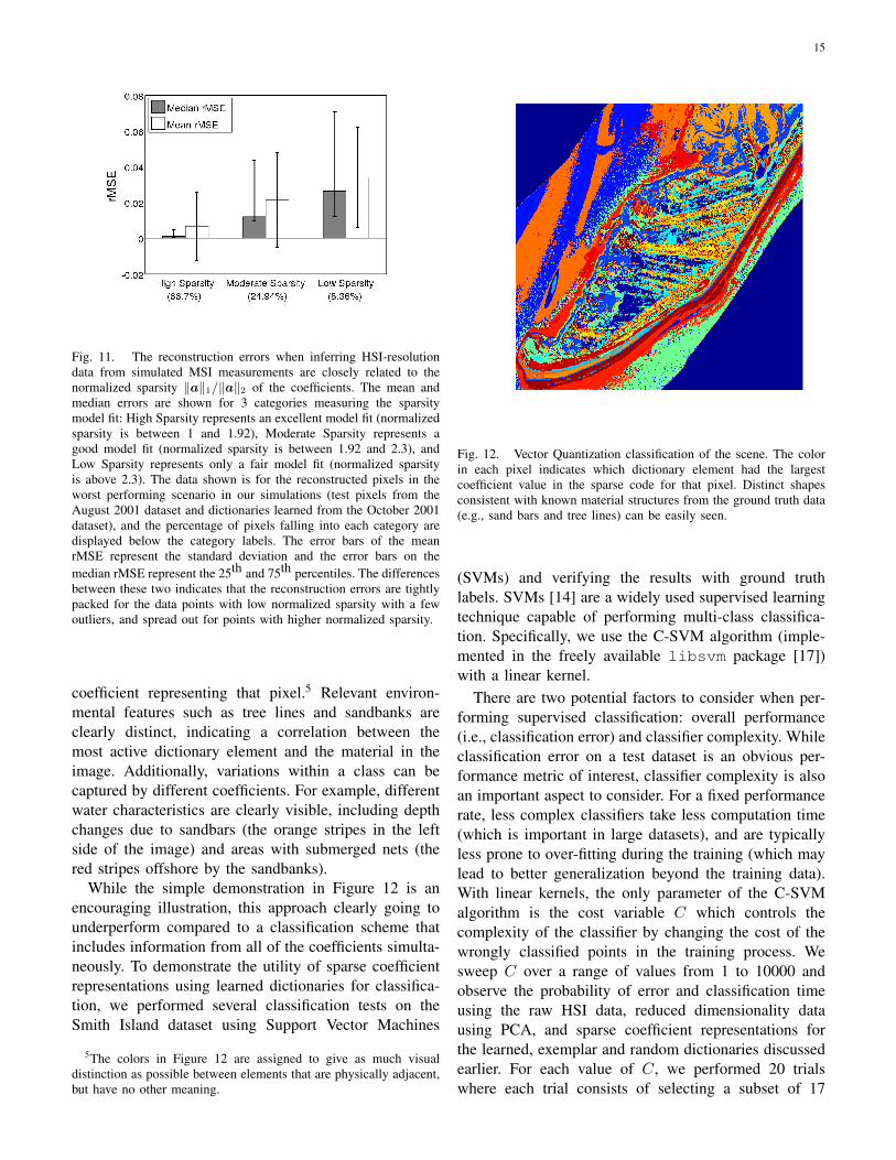
Though the results of the high-resolution reconstruc-tions given above are very encouraging, as with anyengineering application it is important to characterizewhat causes variations in the performance. Figure 11shows a more detailed analysis of the errors for theworst performing case in the above simulations: using

simulated MSI data with a dictionary that was learnedon data taken on a different date from the test data.This analysis quantifies the observation that the betterthe model is at fitting the data, the better we expect theresulting algorithm to perform. Specifically, we groupthe pixels in the test dataset into three groups basedon the (normalized) sparsity of their resulting inferredcoefficients (i.e., how well the data point is fit by asparsity model) measured by ‖a‖1/‖a‖2. The clear trendis that the performance in this task is strongly dependenton how amenable that pixel is to admitting a sparsedecomposition. Fortunately, only a small fraction of thedata (less than 9%) falls into the worst performingcategory. Currently we have not found any quantitativecorrelations between material classes and model fit, butanecdotally we observe that classes such as pine treesand water appear prevalent among the pixels with thelowest rMSE in the reconstruction task, and classessuch as mixed vegetation and mud are more prevalentin the outliers that have higher rMSE. Of course, aninteresting topic of future study would be to understandmore precisely how to modify the model to improvethe fit with the current outliers (and subsequently theperformance on the current task).

We note that there are many other linear inverse prob-lems that may be of interest, including other methods

14

Fig. 10. Reconstructing HSI data from simulated MSI measurements using training and testing data collected on different dates (in differentseasons). Plots show original HSI spectrum in blue (113 bands), simulated coarse HSI spectrum (8 bands), inferred sparse coefficients, andreconstructed HSI spectrum in green. Examples were selected to illustrate a range of recovery performance, from examples of the bestrecovery on top to examples of the worst recovery on the bottom.

for reducing data acquisition resources. For example,in the field of compressed sensing [40], a sparsitymodel is also assumed and data is measured by using acoded aperture that forms each measurement by taking a(generally random) linear combination of the input data.In this case, the original data is recovered by solvingthe same optimization problem as in (5). Indeed, similaracquisition strategies have already been implemented innovel HSI sensors [25], [52]. Looking carefully, the onlydifference between the compressed sensing strategy andthe approach presented above is in the choice of B.The “blurring” choice of B in our experiments shouldactually result in a more difficult reconstruction problemthan when B is chosen to be a random matrix becausethe introduction of randomness will tend to improvethe conditioning of the acquisition operator. We haveperformed similar simulations to the ones above (notshown) using B drawn randomly and independentlyfrom a Bernoulli distribution, and the results indicatethat recovery with similar accuracy is also possible whenusing this learned dictionary.

C. Supervised classification

Clearly one of the most important HSI applications isclassifying the dominant materials present in a pixel [4],

[7], [39]. Because sparse coding is a highly nonlinearoperation that appears to capture different spectral fea-tures by using different dictionary elements (and notjust changing the coefficient values on those elements),we suspect that performing classification on the sparsecoefficients can improve HSI classification performancecompared to classification on the raw data (or otherdimensionality reduced representations such as PCA).Intuition for this approach comes from the well-knownidea in machine learning that expanding a data rep-resentation with a highly nonlinear kernel can serveto separate the data classes and make classificationeasier (especially with a simple linear classifier). Indeed,several researchers have reported that sparse coding inhighly overcomplete learned dictionaries (which is ahighly nonlinear mapping) does improve classificationperformance [34], [49].

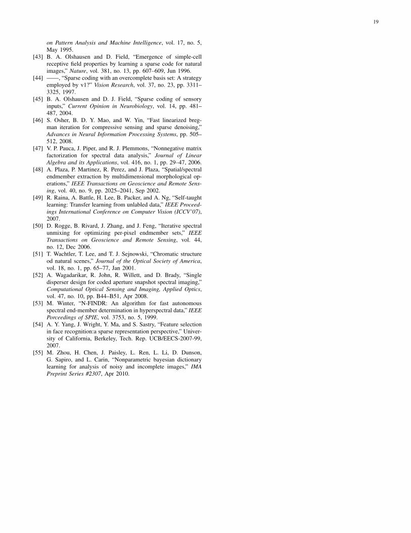
To gain further intuition, consider a very simple classi-fier based on finding the maximum sparse coefficient foreach pixel in the scene. This sparse decomposition withone coefficient can be thought of as a type of vectorquantization (VQ) [42], and the coefficient index canbe used as a rough determination of the class of thepixel. Figure 12 shows a segment of the Smith Islanddataset, where each pixel is independently unmixed andcolored according to the index of the maximum sparse

15

Fig. 11. The reconstruction errors when inferring HSI-resolutiondata from simulated MSI measurements are closely related to thenormalized sparsity ‖a‖1/‖a‖2 of the coefficients. The mean andmedian errors are shown for 3 categories measuring the sparsitymodel fit: High Sparsity represents an excellent model fit (normalizedsparsity is between 1 and 1.92), Moderate Sparsity represents agood model fit (normalized sparsity is between 1.92 and 2.3), andLow Sparsity represents only a fair model fit (normalized sparsityis above 2.3). The data shown is for the reconstructed pixels in theworst performing scenario in our simulations (test pixels from theAugust 2001 dataset and dictionaries learned from the October 2001dataset), and the percentage of pixels falling into each category aredisplayed below the category labels. The error bars of the meanrMSE represent the standard deviation and the error bars on themedian rMSE represent the 25th and 75th percentiles. The differencesbetween these two indicates that the reconstruction errors are tightlypacked for the data points with low normalized sparsity with a fewoutliers, and spread out for points with higher normalized sparsity.

coefficient representing that pixel.5 Relevant environ-mental features such as tree lines and sandbanks areclearly distinct, indicating a correlation between themost active dictionary element and the material in theimage. Additionally, variations within a class can becaptured by different coefficients. For example, differentwater characteristics are clearly visible, including depthchanges due to sandbars (the orange stripes in the leftside of the image) and areas with submerged nets (thered stripes offshore by the sandbanks).

While the simple demonstration in Figure 12 is anencouraging illustration, this approach clearly going tounderperform compared to a classification scheme thatincludes information from all of the coefficients simulta-neously. To demonstrate the utility of sparse coefficientrepresentations using learned dictionaries for classifica-tion, we performed several classification tests on theSmith Island dataset using Support Vector Machines

5The colors in Figure 12 are assigned to give as much visualdistinction as possible between elements that are physically adjacent,but have no other meaning.

Fig. 12. Vector Quantization classification of the scene. The colorin each pixel indicates which dictionary element had the largestcoefficient value in the sparse code for that pixel. Distinct shapesconsistent with known material structures from the ground truth data(e.g., sand bars and tree lines) can be easily seen.

(SVMs) and verifying the results with ground truthlabels. SVMs [14] are a widely used supervised learningtechnique capable of performing multi-class classifica-tion. Specifically, we use the C-SVM algorithm (imple-mented in the freely available libsvm package [17])with a linear kernel.

There are two potential factors to consider when per-forming supervised classification: overall performance(i.e., classification error) and classifier complexity. Whileclassification error on a test dataset is an obvious per-formance metric of interest, classifier complexity is alsoan important aspect to consider. For a fixed performancerate, less complex classifiers take less computation time(which is important in large datasets), and are typicallyless prone to over-fitting during the training (which maylead to better generalization beyond the training data).With linear kernels, the only parameter of the C-SVMalgorithm is the cost variable C which controls thecomplexity of the classifier by changing the cost of thewrongly classified points in the training process. Wesweep C over a range of values from 1 to 10000 andobserve the probability of error and classification timeusing the raw HSI data, reduced dimensionality datausing PCA, and sparse coefficient representations forthe learned, exemplar and random dictionaries discussedearlier. For each value of C, we performed 20 trialswhere each trial consists of selecting a subset of 17

16

Fig. 13. Classification on 22 material classes in the Smith Island dataset. (Left) Average classification error plotted as a function of averageclassification time (as a proxy for classifier complexity) as the complexity parameter of the SVM is varied. Using coefficients from a sparsecode in a learned dictionary as input to the SVM performs essentially as well as using the raw data, but with a classifier 30% less complex.(Right) Average classification error as a function of the training dataset size for each class. The power of the lower complexity classifier isdemonstrated in the ability to generalize better, with sparse coefficients in the learned dictionary clearly showing better performance for thevery small training sets.

pixels from the labeled data for each of the 22 classesto train a new SVM classifier and then testing theclassification performance on the remaining labeled datawithheld from the SVM training.6 We average over alltrials and all 22 classes to find the average classificationerror and average classification time (as a proxy forclassifier complexity). Figure 13 shows the changes inclassification time and probability of classification error.

There are three interesting things to note about theresults in Figure 13. First, while the raw data achievedthe lowest overall error for the range of C tested(P(error)=0.0721), the sparse coefficients in the learneddictionary are nearly as good (P(error)=0.0736) using amuch simpler classifier that operates ∼ 30% faster thanthe SVM on the raw data.7 Second, while PCA reduces

6We choose a training set size of 17 because we want the sameamount of training data per class, and the smallest class has 18labeled samples (leaving one testing pixel for the cross-validation).Average classification performance can be improved significantly onthis dataset when larger training samples are used (but at the expenseof consistent training set sizes per class).

7We note that in other simulations (not shown), the best clas-sification performance of the SVN does not improve when usinga nonlinear kernel such as a radial basis function (though thecomplexity obviously increases compared to the linear kernel). Thisindicates that linear decision boundaries are nearly optimal for thisparticular dataset, and little advantage is gained from a nonlinearmapping of the decision boundary. While in general we would hope tosee lower possible classification error when using sparse coefficients,it appears that nonlinear mappings simply do not add much value tothe decision boundaries for this particular dataset.

the classification time farther then the other approachesdue to its extremely low dimensionality (4 principlecomponents), it performs significantly worse than theraw data or the sparse coefficients. Third, using sparsecoefficients in the random dictionary surprisingly per-forms better (P(error)=0.0838) than sparse coefficientsin the exemplar dictionary (P(error)=0.1262), despitehaving no apparent relevance to material spectra in thescene. While this is counter-intuitive, other recent resultshave shown that projection onto random dictionaries canbe a way to preserve information useful for classifi-cation [34], [54], and it is likely that these dictionar-ies cover the signal space better than random pixelsdrawn from the labeled classes to form the exemplardictionaries. Despite this, the coefficients of the learneddictionary do perform better than the random dictionary,demonstrating the value of the learning process. Finally,we should note that while we only display averageclassification errors, there is a wide variety in the per-class classification errors classes (i.e., some classes areinherently very challenging to distinguish because oftheir similar spectral features [5]). In our observations(not plotted), the relative difficulty of these classes inthe classification task is roughly the same in the differentdata representations.

As mentioned earlier, one advantage of using clas-sifiers with less complexity is that they may generalizebetter from the training data, especially when the trainingdataset is very small. We test the generalization ability of

17

the SVM classification approach described above by re-peating the experiment with variable sizes for the trainingdataset, in the extreme case using only one training pixelper class. We performed and evaluated this simulationin largely the same manner as described above, fixingC = 10, 000 to achieve the lowest classification errorand conservatively using 50 trials (i.e., random selectionsof training data for calculating a new SVM) to mitigatethe increased result sensitivity due to the low trainingset size. Figure 13 plots the results, showing that thesparse coefficients in the learned dictionary do in factgeneralize better than the other methods, outperformingthe other data representations for very small training setsizes (less than 12 training pixels from the total groundtruth data).

IV. CONCLUSIONS

In this work we have shown that a sparse coding modeland the dictionary learning approach described in [44](with minor modifications) can yield valuable represen-tations of HSI data using no a priori information aboutthe dataset. The learned dictionary elements resemblemany of the spectra corresponding to known materialproperties in the scene, and the sparse decompositionof the HSI data using this dictionary shows that thevariations in the surface properties are often sensiblyrepresented. In particular, in contrast with a typicalendmember approach that seeks to contain the HSI datain a convex hull, this learned dictionary captures non-linear material variations directly by forming a locallylinear approximation to the manifolds observed within amaterial class.

The learned dictionaries capture many high-orderstatistics of the data they are learned from, and thisrepresentation showes advantages in applications rele-vant for remote sensing scenarios. For example, whencoupled with a linear inverse problem, this learned dic-tionary demonstrated that HSI-resolution spectra couldbe recovered with remarkable fidelity from (simulated)spectra collected with just MSI-level resolution. Thisperformance is only possible because the learned dictio-naries are capable of effectively capturing the high levelof statistical dependencies inherent in HSI data. Further-more, encouraging results show that the performance onthis task is still very good when there is some mismatchin the statistics because the training and testing data wascollected at different times (i.e., a different season of theyear, with different characteristics in the vegetation andthe atmosphere). While this reconstruction problem wasintended to mimic a realistic and useful data acquisitionscenario, we note that this linear inverse problem frame-work captures many problems of interest (including other

acquisition models such as those in compressed sens-ing [40]). Finally, we showed that the sparse coefficientsfrom this learned dictionary form a useful representationfor performing classification compared to the raw data,yielding classifiers with less complexity that generalizebetter when the training dataset size is very small.

From these results we can conclude that the sparsecoding model is a potentially valuable approach to an-alyzing HSI data, and the learned dictionaries for thismodel form a meaningful representation of the high-order statistics in the HSI data. While this approachshares the same linear model as the common endmemberapproach for spectral unmixing, the different philosophyof representing the data variations directly appears tohave value both in the general understanding of the dataand in specific applications. We believe that this explo-ration (along with the other related results in [16], [28],[29], [55]) demonstrates that more extensive explorationof the utility of this model in HSI is warranted, andimprovements in many specific applications are likely. Inthe future, in addition to more thorough application ofthese ideas to other datasets, it will be valuable to explorethe utility of including increasingly complex modelsin in the learning process. For example, there may bepotential benefits to learning much larger dictionariesthan those shown in this work, learning joint spectral-spatial dictionaries, learning dictionaries customized forspecific applications (such as in [16]), and learning dic-tionaries that attempt to explicitly capture features suchas correlations between pixels and nonlinear variationswithin material classes.

REFERENCES

[1] “The benefits of the 8-spectral bands ofworldview-2,” Mar 2010, available Online athttp://www.digitalglobe.com/downloads/spacecraft/WorldView-2 8-Band Applications Whitepaper.pdf.

[2] M. Aharon, M. Elad, A. Bruckstein, and Y. Katz, “K-SVD:An algorithm for designing of overcomplete dictionaries forsparse representations,” IEEE Proceedings - Special Issue onApplications of Compressive Sensing & Sparse Representation.

[3] M. Aharon, M. Elad, and A. Bruckstein.[4] C. M. Bachmann, “Improving the performance of classifiers

in high-dimensional remote sensing applications: An adaptiveresampling strategy for error-prone exemplars (ARESEPE),”IEEE Transactions on Geoscience and Remote Sensing, vol. 41,no. 9, pp. 2101–2112, Sept 2003.

[5] C. M. Bachmann, T. L. Ainsworth, and R. A. Fusina, “Ex-ploiting manifold geometry in hyperspectral imagery,” IEEETransactions on Geoscience and Remote Sensing, vol. 43, no. 3,pp. 441–454, 2005.

[6] C. M. Bachmann, M. H. Bettenhausen, R. A. Fusina, T. F.Donato, A. L. Russ, J. W. Burke, G. M. Lamela, W. J. Rhea, andB. R. Truitt, “A credit assignment approach to fusing classifiersof multiseasonal hyperspectral imagery,” IEEE Transactions onGeoscience and Remote Sensing, vol. 41, no. 11, pp. 2488–2499, Nov 2003.

18

[7] C. M. Bachmann, T. F. Donato, G. M. Lamela, W. J. Rhea,M. H. Bettenhausen, R. A. Fusina, K. R. D. Bois, J. H. Porter,and B. R. Truitt, “Automatic classification of land cover onsmith island, va, using hymap imagery,” IEEE Transactions onGeoscience and Remote Sensing, vol. 40, no. 10, pp. 2313–2330, Oct 2002.

[8] C. M. Bachmann, T. F. Donato, G. Lamela, J. Rhea, M. Bet-tenhausen, R. A. Fusina, K. D. Bois, J. Porter, and B. Truitt,“Automatic classification of land cover on Smith Island, VA,using HyMAP imagery,” IEEE Transactions on Geoscience andRemote Sensing, vol. 40, no. 10, pp. 2313–2330, 2002.

[9] A. Bateson and B. Curtiss, “A method for manual endmem-ber selection and spectral unmixing,” Remote Sens. Environ.,vol. 55, no. 3, pp. 229–243, Mar 1996.

[10] M. Berman, H. Kiiveri, R. Lagerstrom, A. Ernst, R. Dunne,and J. F. Huntington, “ICE: A statistical approach to itentifyingendmembers in hyperspectral images,” IEEE Transaction onGeoscience and Remote Sensing, vol. 42, no. 10, pp. 2085–2095.

[11] J. Bioucas-Dias and M. Figueiredo, “Alternating direction algo-rithms for constrained sparse regression application to hyper-spectral unmixing,” 2nd IEEE GRSS Workshop on Hyperspec-tral Image and Signal Processing -WHISPERS‘2010, raykjavik,Iceland.

[12] J. Bowles, P. J. Palmadesso, J. A. Antoniadas, M. M. Baumback,and J. L. Rickard, “Use of filter vectors in hyperspectral dataanalysis,” Proceedings of SPIE, Infrared Spaceborne RemoteSensing III, pp. 148–157, 1995.

[13] A. M. Bruckstein, M. Elad, and M. Zibulevsky, “On theuniqueness of nonegative sparse solutions to underdeterminedsparse solutions to underdetermined systems of equations,”IEEE Transactions on Information Theory, vol. 54, no. 11, pp.4813–4820, Nov 2008.

[14] C. Burges, “A tutorial on support vector machines for patternrecognition,” Data Mining and Knowledge Discovery, vol. 2,pp. 121–167, 1998.

[15] E. Candes and J. Romberg, “`1-Magic: Recoveryof sparse signals via convex programming,” 2005,http://www.acm.caltech.edu/l1magic/.

[16] A. Castrodad, Z. Xing, J. Greer, E. Bosch, L. Carin, andG. Sapiro, “Discriminative sparse representations in hyperspec-tral imagery,” IMA Preprint Series #2319, Mar 2010.

[17] C.-C. Chang and C.-J. Lin, LIBSVM: a library forsupport vector machines, 2001, software available athttp://www.csie.ntu.edu.tw/ cjlin/libsvm.

[18] A. S. Charles, B. A. Olshausen, and C. J. Rozell, “Sparse cod-ing for spectral signatures in hyperspectral images,” AsilomarConference on Signals, Systems and Computers, 2010.

[19] S. S. Chen, D. L. Donoho, and M. A. Saunders, “Atomicdecomposition by basis pursuit,” SIAM Review, vol. 43, no. 1,pp. 129–159, 2001.

[20] M. Elad, M. Figueiredo, and Y. Ma, “On the role of sparse andredundant representations in image processing,” IEEE Proceed-ings - Special Issue on Applications of Compressive Sensing &Sparse Representation, Oct 2008.

[21] S. Erard, P. Drossart, and G. Piccioni, “Multivariate analysisof visible and infrared thermal imaging spectrometer (virtis)venus express nightside and limb observations,” Journal ofGeophysical Research, vol. 114, 2009.

[22] M. A. T. Figueiredo, R. D. Nowak, and S. J. Wright, “Gradientprojection for sparse reconstruction: Application to compressedsensing and other inverse problems,” IEEE Journal of SelectedTopics in Signal Processing, 2007.

[23] O. Forni, S. M. Clegg, R. C. Wiens, and S. M. anc O. Gasnault,“Multivariate analysis of ChemCam first calibration samples,”40th Lunar and Planetary Science Conference, vol. 1523, 2009.

[24] O. Forni, F. Poulet, J.-P. Bibring, S. Erard, C. Gomez,Y. Langevin, B. Gondet, and Omega Team, “Component sepa-ration of omega spectra with ica,” Lunar and Planetary ScienceTechnical Report, vol. 1623, 2005.

[25] M. E. Gehm, R. John, D. J. Brady, R. M. Willett, and T. J.Schulz, “Single-shot compressive spectral imaging with dual-disperser architecture,” Optics Express, vol. 15, no. 21, pp.14 013–14 026, Oct 2007.

[26] Q. Geng, H. Wang, and J. Wright, “On thelocal correctness of `1-minimization for dic-tionary learning,” no. arXiv:1101.5672v1, 2011,http://arxiv4.library.cornell.edu/pdf/1101.5672v1.

[27] C. Gomez, H. L. Borgne, P. Allemand, C. Delacourt, andP. Ledru, “N-FindR method versus independent componentanalysis for lithological identification in hyperspectral imagery,”International Journal of Remote Sensing, vol. 28, no. 23, pp.5315–5338, Jun 2007.

[28] J. Greer, “Sparse demixing,” IEEE Proceedings of SPIE, vol.7695, May 2010.

[29] Z. Guo, T. Wittman, and S. Osher, “L1 unmixing and itsapplication to hyperspectral image enhancement,” Proc. SPIEConference on Algorithms and Technologies for Multispectral,Hyperspectral, and Ultraspectral Imagery XV, orlando, Florida.

[30] E. T. Hale, W. Yin, and Y. Zhang, “A fixed-point continuationmethod for l1-regularized minimization with applications tocompressed sensing,” Rice University Department of Computa-tional and Applied Mathematics, Tech. Rep., Jul 2007.

[31] P. O. Hoyer, “Non-negative matrix factorization with sparsenessconstraints,” Journal of Machine Learning Research, vol. 5,no. 9, pp. 1457–1469, Nov 2004.

[32] A. Ifarraguerri and C.-I. Chang, “Multispectral and hyperspec-tral image analysis with convex cones,” IEEE Transactions onGeoscience and Remote Sensing, vol. 37, no. 2, pp. 756–770,Mar 1999.

[33] M.-D. Iordache, J. M. B. Dias, and A. Plaza, “Sparse unmixingof hyperspectral data,” IEEE Transactions on Geoscience andRemote Sensing, 2010.

[34] K. Jarrett, K. Kavukcuoglu, M. Ranzato, and Y. LeCun, “Whatis the best multi-stage architecture for object recognition?”IEEE Proceedings International Conference on Computer Vi-sion (ICCV’09), 2009.

[35] S. Jia and Y. Qian, “Constrained nonnegative matrix fac-torization for hyperspectral imaging,” IEEE Transactions onGeoscience and Remote Sensing, vol. 47, no. 1, pp. 161–173,Jan 2009.

[36] J. P. Kerkes and J. R. Schott, “Hyperspectral imaging systems,”in Hyperspectral Data Exploitation: Theory and Applications,C.-I. Chang, Ed. John Wiley & Sons, Inc., 2007, pp. 19–45.

[37] N. Keshava and J. F. Mustard, “Spectral unmixing,” IEEE SignalProceesing Magazine, vol. 19, no. 1, pp. 44–57.

[38] S.-J. Kim, K. Koh, M. Lustig, S. Boyd, and D. Gorinevsky,“An interior-point method for large scale l1-regularized leastsquares,” IEEE Journal on Selected Topics in Signal Processing,vol. 1, no. 4, pp. 606–617, Dec 2007.

[39] D. Manolakis and G. Shaw, “Detection algorithms for hyper-spectral imaging applications,” IEEE Proceesings on SignalProcessing, vol. 19, no. 1, pp. 29–43, Jan 2002.

[40] R. Maraniuk, “Compressive sensing,” IEEE Signal ProcessingMagazine, vol. 24, no. 4, pp. 118–121, Jul 2007.

[41] S. Moussaoui, H. Hauksdottir, F. Schmidt, C. Jutten, J. Chanus-sot, D. Brie, S. Doute, and J. A. Benediksson, “On the de-composition of mars hyperspectral data by ica and bayesianpositive source separation,” Neurocomputing, vol. 71, no. 10-12, pp. 2194–2208, Jun 2008.

[42] K. L. Oehler and R. M. Gray, “Combining image compressionand classification using vector quantization,” IEEE Transactions

19

on Pattern Analysis and Machine Intelligence, vol. 17, no. 5,May 1995.

[43] B. A. Olshausen and D. Field, “Emergence of simple-cellreceptive field properties by learning a sparse code for naturalimages,” Nature, vol. 381, no. 13, pp. 607–609, Jun 1996.

[44] ——, “Sparse coding with an overcomplete basis set: A strategyemployed by v1?” Vision Research, vol. 37, no. 23, pp. 3311–3325, 1997.

[45] B. A. Olshausen and D. J. Field, “Sparse coding of sensoryinputs,” Current Opinion in Neurobiology, vol. 14, pp. 481–487, 2004.

[46] S. Osher, B. D. Y. Mao, and W. Yin, “Fast linearized breg-man iteration for compressive sensing and sparse denoising,”Advances in Neural Information Processing Systems, pp. 505–512, 2008.

[47] V. P. Pauca, J. Piper, and R. J. Plemmons, “Nonnegative matrixfactorization for spectral data analysis,” Journal of LinearAlgebra and its Applications, vol. 416, no. 1, pp. 29–47, 2006.

[48] A. Plaza, P. Martinez, R. Perez, and J. Plaza, “Spatial/spectralendmember extraction by multidimensional morphological op-erations,” IEEE Transactions on Geoscience and Remote Sens-ing, vol. 40, no. 9, pp. 2025–2041, Sep 2002.

[49] R. Raina, A. Battle, H. Lee, B. Packer, and A. Ng, “Self-taughtlearning: Transfer learning from unlabled data,” IEEE Proceed-ings International Conference on Computer Vision (ICCV’07),2007.

[50] D. Rogge, B. Rivard, J. Zhang, and J. Feng, “Iterative spectralunmixing for optimizing per-pixel endmember sets,” IEEETransactions on Geoscience and Remote Sensing, vol. 44,no. 12, Dec 2006.

[51] T. Wachtler, T. Lee, and T. J. Sejnowski, “Chromatic structureod natural scenes,” Journal of the Optical Society of America,vol. 18, no. 1, pp. 65–77, Jan 2001.

[52] A. Wagadarikar, R. John, R. Willett, and D. Brady, “Singledisperser design for coded aperture snapshot spectral imaging,”Computational Optical Sensing and Imaging, Applied Optics,vol. 47, no. 10, pp. B44–B51, Apr 2008.

[53] M. Winter, “N-FINDR: An algorithm for fast autonomousspectral end-member determination in hyperspectral data,” IEEEPorceedings of SPIE, vol. 3753, no. 5, 1999.

[54] A. Y. Yang, J. Wright, Y. Ma, and S. Sastry, “Feature selectionin face recognition:a sparse representation perspective,” Univer-sity of California, Berkeley, Tech. Rep. UCB/EECS-2007-99,2007.

[55] M. Zhou, H. Chen, J. Paisley, L. Ren, L. Li, D. Dunson,G. Sapiro, and L. Carin, “Nonparametric bayesian dictionarylearning for analysis of noisy and incomplete images,” IMAPreprint Series #2307, Apr 2010.