learning stable nonlinear dynamical systems with gaussian ... · learning stable nonlinear...

IEEE TRANSACTIONS ON ROBOTICS, VOL. 27, NO. 5, OCTOBER 2011 943

Learning Stable Nonlinear Dynamical SystemsWith Gaussian Mixture Models

S. Mohammad Khansari-Zadeh and Aude Billard

Abstract—This paper presents a method to learn discrete robotmotions from a set of demonstrations. We model a motion as a non-linear autonomous (i.e., time-invariant) dynamical system (DS) anddefine sufficient conditions to ensure global asymptotic stability atthe target. We propose a learning method, which is called StableEstimator of Dynamical Systems (SEDS), to learn the parametersof the DS to ensure that all motions closely follow the demonstra-tions while ultimately reaching and stopping at the target. Time-invariance and global asymptotic stability at the target ensures thatthe system can respond immediately and appropriately to pertur-bations that are encountered during the motion. The method isevaluated through a set of robot experiments and on a library ofhuman handwriting motions.

Index Terms—Dynamical systems (DS), Gaussian mixturemodel, imitation learning, point-to-point motions, stabilityanalysis.

I. INTRODUCTION

W E consider modeling of point-to-point motions, i.e.,movements in space stopping at a given target [1].

Modeling point-to-point motions provides basic componentsfor robot control, whereby more complex tasks can be decom-posed into sets of point-to-point motions [1], [2]. As an example,consider the standard “pick-and-place” task: First, reach for theitem, then after grasping, move to the target location, and finally,return home after release.

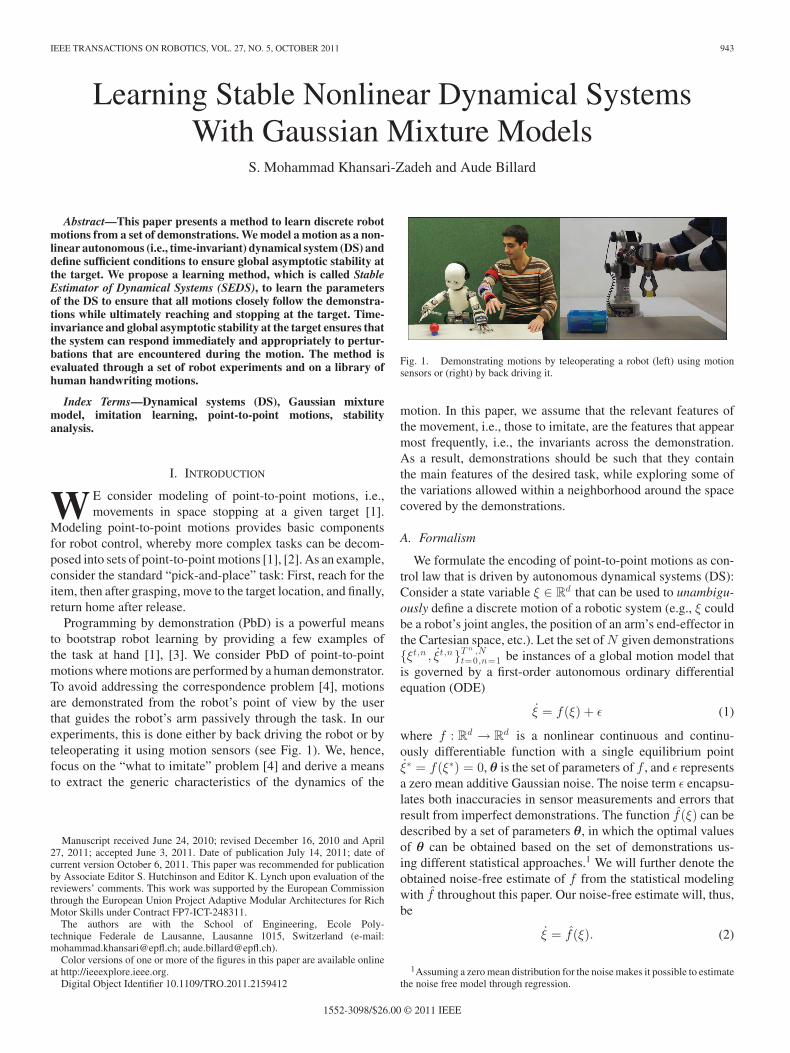
Programming by demonstration (PbD) is a powerful meansto bootstrap robot learning by providing a few examples ofthe task at hand [1], [3]. We consider PbD of point-to-pointmotions where motions are performed by a human demonstrator.To avoid addressing the correspondence problem [4], motionsare demonstrated from the robot’s point of view by the userthat guides the robot’s arm passively through the task. In ourexperiments, this is done either by back driving the robot or byteleoperating it using motion sensors (see Fig. 1). We, hence,focus on the “what to imitate” problem [4] and derive a meansto extract the generic characteristics of the dynamics of the

Manuscript received June 24, 2010; revised December 16, 2010 and April27, 2011; accepted June 3, 2011. Date of publication July 14, 2011; date ofcurrent version October 6, 2011. This paper was recommended for publicationby Associate Editor S. Hutchinson and Editor K. Lynch upon evaluation of thereviewers’ comments. This work was supported by the European Commissionthrough the European Union Project Adaptive Modular Architectures for RichMotor Skills under Contract FP7-ICT-248311.

The authors are with the School of Engineering, Ecole Poly-technique Federale de Lausanne, Lausanne 1015, Switzerland (e-mail:[email protected]; [email protected]).

Color versions of one or more of the figures in this paper are available onlineat http://ieeexplore.ieee.org.

Digital Object Identifier 10.1109/TRO.2011.2159412

Fig. 1. Demonstrating motions by teleoperating a robot (left) using motionsensors or (right) by back driving it.

motion. In this paper, we assume that the relevant features ofthe movement, i.e., those to imitate, are the features that appearmost frequently, i.e., the invariants across the demonstration.As a result, demonstrations should be such that they containthe main features of the desired task, while exploring some ofthe variations allowed within a neighborhood around the spacecovered by the demonstrations.

A. Formalism

We formulate the encoding of point-to-point motions as con-trol law that is driven by autonomous dynamical systems (DS):Consider a state variable ξ ∈ R

d that can be used to unambigu-ously define a discrete motion of a robotic system (e.g., ξ couldbe a robot’s joint angles, the position of an arm’s end-effector inthe Cartesian space, etc.). Let the set of N given demonstrations{ξt,n , ξt,n}T n ,N

t=0,n=1 be instances of a global motion model thatis governed by a first-order autonomous ordinary differentialequation (ODE)

ξ = f(ξ) + ε (1)

where f : Rd → R

d is a nonlinear continuous and continu-ously differentiable function with a single equilibrium pointξ∗ = f(ξ∗) = 0, θ is the set of parameters of f , and ε representsa zero mean additive Gaussian noise. The noise term ε encapsu-lates both inaccuracies in sensor measurements and errors thatresult from imperfect demonstrations. The function f(ξ) can bedescribed by a set of parameters θ, in which the optimal valuesof θ can be obtained based on the set of demonstrations us-ing different statistical approaches.1 We will further denote theobtained noise-free estimate of f from the statistical modelingwith f throughout this paper. Our noise-free estimate will, thus,be

ξ = f(ξ). (2)

1Assuming a zero mean distribution for the noise makes it possible to estimatethe noise free model through regression.

1552-3098/$26.00 © 2011 IEEE

944 IEEE TRANSACTIONS ON ROBOTICS, VOL. 27, NO. 5, OCTOBER 2011

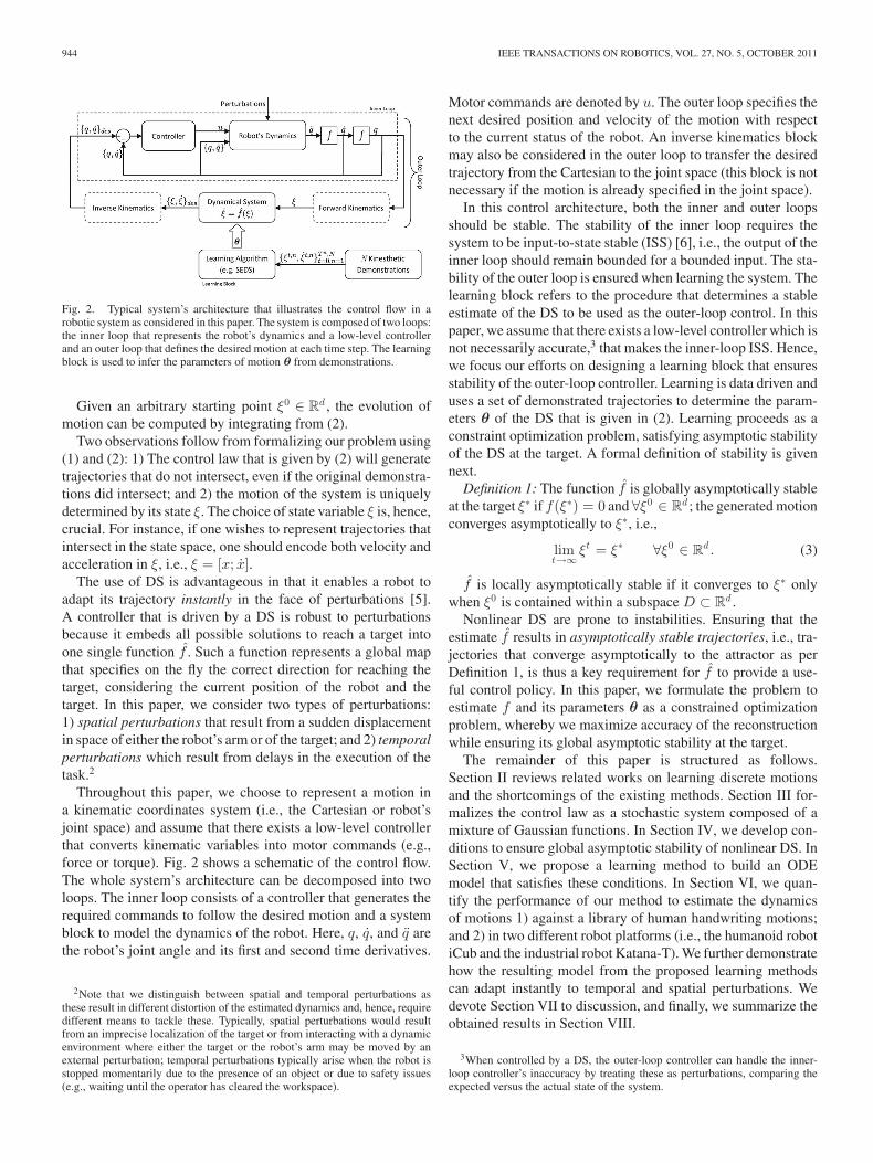
Fig. 2. Typical system’s architecture that illustrates the control flow in arobotic system as considered in this paper. The system is composed of two loops:the inner loop that represents the robot’s dynamics and a low-level controllerand an outer loop that defines the desired motion at each time step. The learningblock is used to infer the parameters of motion θ from demonstrations.

Given an arbitrary starting point ξ0 ∈ Rd , the evolution of

motion can be computed by integrating from (2).Two observations follow from formalizing our problem using

(1) and (2): 1) The control law that is given by (2) will generatetrajectories that do not intersect, even if the original demonstra-tions did intersect; and 2) the motion of the system is uniquelydetermined by its state ξ. The choice of state variable ξ is, hence,crucial. For instance, if one wishes to represent trajectories thatintersect in the state space, one should encode both velocity andacceleration in ξ, i.e., ξ = [x; x].

The use of DS is advantageous in that it enables a robot toadapt its trajectory instantly in the face of perturbations [5].A controller that is driven by a DS is robust to perturbationsbecause it embeds all possible solutions to reach a target intoone single function f . Such a function represents a global mapthat specifies on the fly the correct direction for reaching thetarget, considering the current position of the robot and thetarget. In this paper, we consider two types of perturbations:1) spatial perturbations that result from a sudden displacementin space of either the robot’s arm or of the target; and 2) temporalperturbations which result from delays in the execution of thetask.2

Throughout this paper, we choose to represent a motion ina kinematic coordinates system (i.e., the Cartesian or robot’sjoint space) and assume that there exists a low-level controllerthat converts kinematic variables into motor commands (e.g.,force or torque). Fig. 2 shows a schematic of the control flow.The whole system’s architecture can be decomposed into twoloops. The inner loop consists of a controller that generates therequired commands to follow the desired motion and a systemblock to model the dynamics of the robot. Here, q, q, and q arethe robot’s joint angle and its first and second time derivatives.

2Note that we distinguish between spatial and temporal perturbations asthese result in different distortion of the estimated dynamics and, hence, requiredifferent means to tackle these. Typically, spatial perturbations would resultfrom an imprecise localization of the target or from interacting with a dynamicenvironment where either the target or the robot’s arm may be moved by anexternal perturbation; temporal perturbations typically arise when the robot isstopped momentarily due to the presence of an object or due to safety issues(e.g., waiting until the operator has cleared the workspace).

Motor commands are denoted by u. The outer loop specifies thenext desired position and velocity of the motion with respectto the current status of the robot. An inverse kinematics blockmay also be considered in the outer loop to transfer the desiredtrajectory from the Cartesian to the joint space (this block is notnecessary if the motion is already specified in the joint space).

In this control architecture, both the inner and outer loopsshould be stable. The stability of the inner loop requires thesystem to be input-to-state stable (ISS) [6], i.e., the output of theinner loop should remain bounded for a bounded input. The sta-bility of the outer loop is ensured when learning the system. Thelearning block refers to the procedure that determines a stableestimate of the DS to be used as the outer-loop control. In thispaper, we assume that there exists a low-level controller which isnot necessarily accurate,3 that makes the inner-loop ISS. Hence,we focus our efforts on designing a learning block that ensuresstability of the outer-loop controller. Learning is data driven anduses a set of demonstrated trajectories to determine the param-eters θ of the DS that is given in (2). Learning proceeds as aconstraint optimization problem, satisfying asymptotic stabilityof the DS at the target. A formal definition of stability is givennext.

Definition 1: The function f is globally asymptotically stableat the target ξ∗ if f(ξ∗) = 0 and ∀ξ0 ∈ R

d ; the generated motionconverges asymptotically to ξ∗, i.e.,

limt→∞

ξt = ξ∗ ∀ξ0 ∈ Rd . (3)

f is locally asymptotically stable if it converges to ξ∗ onlywhen ξ0 is contained within a subspace D ⊂ R

d .Nonlinear DS are prone to instabilities. Ensuring that the

estimate f results in asymptotically stable trajectories, i.e., tra-jectories that converge asymptotically to the attractor as perDefinition 1, is thus a key requirement for f to provide a use-ful control policy. In this paper, we formulate the problem toestimate f and its parameters θ as a constrained optimizationproblem, whereby we maximize accuracy of the reconstructionwhile ensuring its global asymptotic stability at the target.

The remainder of this paper is structured as follows.Section II reviews related works on learning discrete motionsand the shortcomings of the existing methods. Section III for-malizes the control law as a stochastic system composed of amixture of Gaussian functions. In Section IV, we develop con-ditions to ensure global asymptotic stability of nonlinear DS. InSection V, we propose a learning method to build an ODEmodel that satisfies these conditions. In Section VI, we quan-tify the performance of our method to estimate the dynamicsof motions 1) against a library of human handwriting motions;and 2) in two different robot platforms (i.e., the humanoid robotiCub and the industrial robot Katana-T). We further demonstratehow the resulting model from the proposed learning methodscan adapt instantly to temporal and spatial perturbations. Wedevote Section VII to discussion, and finally, we summarize theobtained results in Section VIII.

3When controlled by a DS, the outer-loop controller can handle the inner-loop controller’s inaccuracy by treating these as perturbations, comparing theexpected versus the actual state of the system.

KHANSARI-ZADEH AND BILLARD: LEARNING STABLE NONLINEAR DYNAMICAL SYSTEMS WITH GAUSSIAN MIXTURE MODELS 945

II. RELATED WORKS

Statistical approaches to modeling robot motion have becomeincreasingly popular as a means to deal with the noise inherentin any mechanical system. They have proved to be interesting al-ternatives to classical control and planning approaches when theunderlying model cannot be well estimated. Traditional meansof encoding trajectories is based on spline decomposition af-ter averaging across training trajectories [7]–[10]. While thismethod is a useful tool for quick and efficient decompositionand generalization over a given set of trajectories, it is, how-ever, heavily dependent on heuristics to segment and align thetrajectories and gives a poor estimate of nonlinear trajectories.

Some alternatives to spline-based techniques perform regres-sion over a nonlinear estimate of the motion that is based onGaussian kernels [2], [11], [12]. These methods provide pow-erful means to encode arbitrary multidimensional nonlinear tra-jectories. However, similar to spline encoding, these approachesdepend on explicit time indexing and virtually operate in an openloop. Time dependence makes these techniques very sensitiveto both temporal and spatial perturbations. To compensate forthis deficiency,4 one requires a heuristic to reindex the new tra-jectory in time, while simultaneously optimizing a measure ofhow good the new trajectory follows the desired one. To finda good heuristic is highly task-dependent and a nontrivial task,and becomes particularly nonintuitive in high-dimensional statespaces.

Coates et al. [13] proposed an Expectation Maximization(EM) algorithm that uses an (extended) Kalman smoother tofollow a desired trajectory from the demonstrations. They usedynamic programming to infer the desired target trajectory anda time alignment of all demonstrations. Their algorithm alsolearns a local model of the robot’s dynamics along the desiredtrajectory. Although this algorithm is shown to be an efficientmethod to learn complex motions, it is time dependent and, thus,shares the disadvantages that are mentioned earlier.

DS have been advocated as a powerful alternative to mod-eling robot motions [5], [14]. Existing approaches to the sta-tistical estimation of f in (2) use either Gaussian Process Re-gression (GPR) [15], Locally Weighted Projection Regression(LWPR) [16], or Gaussian Mixture Regression (GMR) [14],where the parameters of the Gaussian Mixture are optimizedthrough EM [17]. GMR and GPR find a locally optimal modelof f by maximizing the likelihood that the complete model rep-resents the data well, while LWPR minimizes the mean squareerror (MSE) between the estimates and the data (for a detaileddiscussion on these methods, see [18]).

Because all of the aforementioned methods do not optimizeunder the constraint of making the system stable at the attractor,they are not guaranteed to result in a stable estimate of the mo-tion. In practice, they fail to ensure global stability, and they alsorarely ensure local stability of f (see Definition 1). Such esti-mates of the motion may, hence, converge to spurious attractorsor miss the target (diverging/unstable behavior) even when esti-

4If one is to model only time-dependent motions, i.e., motions that are deemedto be performed in a fixed amount of time, then one may prefer a time-dependentencoding.

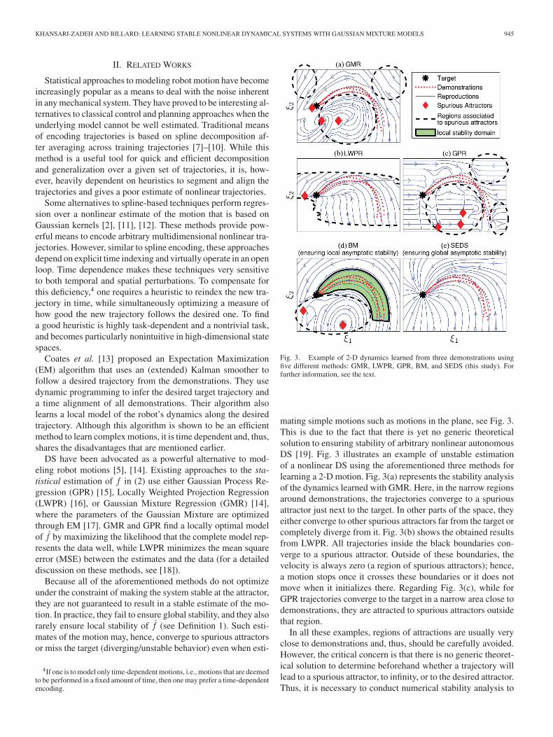
Fig. 3. Example of 2-D dynamics learned from three demonstrations usingfive different methods: GMR, LWPR, GPR, BM, and SEDS (this study). Forfurther information, see the text.

mating simple motions such as motions in the plane, see Fig. 3.This is due to the fact that there is yet no generic theoreticalsolution to ensuring stability of arbitrary nonlinear autonomousDS [19]. Fig. 3 illustrates an example of unstable estimationof a nonlinear DS using the aforementioned three methods forlearning a 2-D motion. Fig. 3(a) represents the stability analysisof the dynamics learned with GMR. Here, in the narrow regionsaround demonstrations, the trajectories converge to a spuriousattractor just next to the target. In other parts of the space, theyeither converge to other spurious attractors far from the target orcompletely diverge from it. Fig. 3(b) shows the obtained resultsfrom LWPR. All trajectories inside the black boundaries con-verge to a spurious attractor. Outside of these boundaries, thevelocity is always zero (a region of spurious attractors); hence,a motion stops once it crosses these boundaries or it does notmove when it initializes there. Regarding Fig. 3(c), while forGPR trajectories converge to the target in a narrow area close todemonstrations, they are attracted to spurious attractors outsidethat region.

In all these examples, regions of attractions are usually veryclose to demonstrations and, thus, should be carefully avoided.However, the critical concern is that there is no generic theoret-ical solution to determine beforehand whether a trajectory willlead to a spurious attractor, to infinity, or to the desired attractor.Thus, it is necessary to conduct numerical stability analysis to


locate the region of attraction of the desired target which maynever exist or may be very narrow.

The Dynamic Movement Primitives (DMP) [20] offer amethod by which a nonlinear DS can be estimated while en-suring global stability at an attractor point. Global stability isensured through the use of linear DS that takes precedence overthe nonlinear modulation to ensure stability at the end of themotion. The switch from nonlinear to linear dynamics proceedssmoothly according to a phase variable that acts as an implicitclock. Such an implicit time dependence requires a heuristicsto reset the phase variable in the face of temporal perturbations.When learning from a single demonstration, DMP offers a ro-bust and precise means of encoding a complex dynamics. Here,we take a different approach in which we aim at learning a gen-eralized dynamics from multiple demonstrations. We also aimto ensure time independence, and hence robustness to temporalperturbations. Learning also proceeds from extracting corre-lation across several dimensions. While DMP learns a modelfor each dimension separately, we here model a single multi-dimensional model. The approach that we propose is, hence,complementary to DMP. The choice between using DMP orstable estimator of dynamical systems (SEDS) to model a mo-tion is application dependent. For example, when the motion isintrinsically time dependent and only a single demonstration isavailable, one may use DMP to model the motion. In contrast,when the motion is time independent and when learning frommultiple demonstrations, one may opt to use SEDS. For a moredetailed discussion of these issues and for quantitative compar-isons across time-dependent and time-independent encoding ofmotions using DS, see [5] and [21].

In our prior work [14], we developed a hybrid controller thatis composed of two DS working concurrently in end-effectorand joint angle spaces, resulting in a controller that has nosingularities. While this approach was able to adapt online tosudden displacements of the target or unexpected movement ofthe arm during the motion, the model remained time dependentbecause, similarly to DMP, it relied on a stable linear DS with afixed internal clock.

We, then, considered an alternative DS approach that is basedon the hidden Markov model and GMR [22]. The method thatis presented here is time independent and, thus, robust to tem-poral perturbations. Asymptotic stability could, however, notbe ensured. Sole a brief verification to avoid large instabilitieswas done by evaluating the eigenvalues of each linear DS andensuring that they all have negative real parts. As stated in [22]and as we will show in Section IV, asking that all eigenvaluesbe negative is not a sufficient condition to ensure stability of thecomplete system (see, e.g., Fig. 5).

In [21] and [23], we proposed a heuristics to build iteratively alocally stable estimate of nonlinear DS. This heuristics requiresone to increase the number of Gaussians and retrain the mix-ture using EM iteratively until stability can be ensured. Stabilitywas tested numerically. This approach suffered from the factthat it was not ensured to find a (even locally) stable estimateand that it gave no explicit constraint on the form of the Gaus-sians to ensure stability. The model had a limited domain ofapplicability because of its local stability, and it was also com-

putationally intensive, making it difficult to apply the method inhigh dimensions.

In [18], we proposed an iterative method, which is calledBinary Merging (BM), to construct a mixture of Gaussians soas to ensure local asymptotic stability at the target; hence, themodel can be only applied in a region close to demonstrations[see Fig. 3(d)]. Although this study provided sufficient condi-tions to make DS locally stable, similar to [23], it still relied ondetermining numerically the stability region and had a limitedregion of applicability.

In this paper, we develop a formal analysis of stability andformulate explicit constraints on the parameters of the mixtureto ensure global asymptotic stability of DS. This approach pro-vides a sound ground for the estimation of nonlinear DS whichis not heuristic driven and, thus, has the potential for much largersets of applications, such as the estimation of second-order dy-namics and for control of multidegrees of freedom (multi-DOF)robots as we demonstrate here. Fig. 3(e) represents results thatare obtained in this paper. Being globally asymptotically sta-ble, all trajectories converge to the target. This ensures that thetask can be successfully accomplished starting from any pointin the operational space with no need to reindex or rescale. Notethat the stability analysis that we presented here was publishedin a preliminary form in [5]. This paper largely extends thiswork by 1) having a more depth discussion on stability; 2) byproposing two objective functions to learn parameters of DSand comparing their pros and cons; 3) by having a more de-tailed comparison of the performance of the proposed methodwith BM and three best regression methods to estimate motiondynamics, namely GMR, LWPR, and GPR; and 4) by havingmore robot experiments.

III. MULTIVARIATE REGRESSION

We use a probabilistic framework and model f via a finitemixture of Gaussian functions. Mixture modeling is a popularapproach for density approximation [24], and it allows a user todefine an appropriate model through a tradeoff between modelcomplexity and variations of the available training data. Mixturemodeling is a method that builds a coarse representation of thedata density through a fixed number (usually lower than 10) ofmixture components. An optimal number of components can befound using various methods, such as the Bayesian informationcriterion (BIC) [25], the Akaike information criterion (AIC)[26], the deviance information criterion (DIC) [27], that penalizea large increase in the number of parameters when it only offersa small gain in the likelihood of the model.

While nonparametric methods, such as Gaussian Process orvariants on these, offer optimal regression [15], [28], they sufferfrom the curse of dimensionality. Indeed, computing the esti-mate regressor f grows linearly with the number of data points,making such an estimation inadequate for on-the-fly recompu-tation of the trajectory in the face of perturbations. There ex-ists various sparse techniques to reduce the sensitivity of thesemethods to the number of data points. However, these tech-niques either become parametric by predetermining the optimalnumber of data points [29], or they rely on a heuristic such as


information gain to determine the optimal subset of data points[30]. These heuristics resemble that offered by the BIC, DIC, orAIC criteria.

Estimating f via a finite mixture of Gaussian functions, theunknown parameters of f become the prior πk , the mean μk

and the covariance matrices Σk of the k = 1 . . . K Gaussianfunctions (i.e., θk = {πk , μk ,Σk} and θ = {θ1 . . . θK }). Themean and the covariance matrices of a Gaussian k are definedby

μk =

(μk

ξ

μkξ

), Σk =

(Σk

ξ Σkξ ξ

Σkξξ

Σkξ

). (4)

Given a set of N demonstrations {ξt,n , ξt,n}T n ,Nt=0,n=1 , each

recorded point in the trajectories [ξt,n , ξt,n ] is associated with aprobability density function P(ξt,n , ξt,n ):

P(ξt,n , ξt,n ;θ) =K∑

k=1

P(k)P(ξt,n , ξt,n |k){ ∀n ∈ 1 . . . N

t ∈ 0 . . . T n

(5)where P(k) = πk is the prior, and P(ξt,n , ξt,n |k) is the condi-tional probability density function that is given by

P(ξt,n , ξt,n |k) = N (ξt,n , ξt,n ;μk ,Σk )

=1√

(2π)2d |Σk |e−

12 ([ξ t , n ,ξ t , n ]−μk )T (Σk )−1 ([ξ t , n ,ξ t , n ]−μk ) . (6)

Taking the posterior mean estimate of P(ξ|ξ) yields (as de-scribed in [31])

ξ =K∑

k=1

P(k)P(ξ|k)∑Ki=1 P(i)P(ξ|i)

(μk

ξ+ Σk

ξξ

(Σk

ξ

)−1(ξ − μk

ξ

)). (7)

The notation of (7) can be simplified through a change ofvariable. Let us define⎧⎪⎪⎪⎨

⎪⎪⎪⎩

Ak = Σkξξ

(Σkξ )−1

bk = μkξ− Akμk

ξ

hk (ξ) = P(k)P(ξ |k)∑K

i = 1P(i)P(ξ |i)

.

(8)

The substitution of (8) into (7) yields

ξ = f(ξ) =K∑

k=1

hk (ξ)(Akξ + bk ). (9)

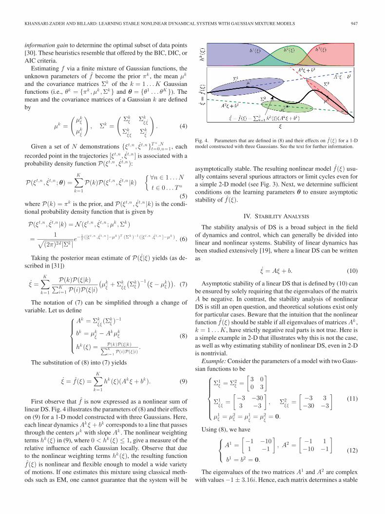
First observe that f is now expressed as a nonlinear sum oflinear DS. Fig. 4 illustrates the parameters of (8) and their effectson (9) for a 1-D model constructed with three Gaussians. Here,each linear dynamics Akξ + bk corresponds to a line that passesthrough the centers μk with slope Ak . The nonlinear weightingterms hk (ξ) in (9), where 0 < hk (ξ) ≤ 1, give a measure of therelative influence of each Gaussian locally. Observe that dueto the nonlinear weighting terms hk (ξ), the resulting functionf(ξ) is nonlinear and flexible enough to model a wide varietyof motions. If one estimates this mixture using classical meth-ods such as EM, one cannot guarantee that the system will be

Fig. 4. Parameters that are defined in (8) and their effects on f (ξ) for a 1-Dmodel constructed with three Gaussians. See the text for further information.

asymptotically stable. The resulting nonlinear model f(ξ) usu-ally contains several spurious attractors or limit cycles even fora simple 2-D model (see Fig. 3). Next, we determine sufficientconditions on the learning parameters θ to ensure asymptoticstability of f(ξ).

IV. STABILITY ANALYSIS

The stability analysis of DS is a broad subject in the fieldof dynamics and control, which can generally be divided intolinear and nonlinear systems. Stability of linear dynamics hasbeen studied extensively [19], where a linear DS can be writtenas

ξ = Aξ + b. (10)

Asymptotic stability of a linear DS that is defined by (10) canbe ensured by solely requiring that the eigenvalues of the matrixA be negative. In contrast, the stability analysis of nonlinearDS is still an open question, and theoretical solutions exist onlyfor particular cases. Beware that the intuition that the nonlinearfunction f(ξ) should be stable if all eigenvalues of matrices Ak ,k = 1 . . . K, have strictly negative real parts is not true. Here isa simple example in 2-D that illustrates why this is not the case,as well as why estimating stability of nonlinear DS, even in 2-Dis nontrivial.

Example: Consider the parameters of a model with two Gaus-sian functions to be⎧⎪⎪⎪⎪⎪⎨

⎪⎪⎪⎪⎪⎩

Σ1ξ = Σ2

ξ =[

3 00 3

]

Σ1ξ ξ

=[−3 −303 −3

], Σ2

ξ ξ=

[−3 3−30 −3

]μ1

ξ = μ2ξ = μ1

ξ= μ2

ξ= 0.

(11)

Using (8), we have⎧⎨⎩A1 =

[−1 −101 −1

], A2 =

[−1 1−10 −1

]b1 = b2 = 0.

(12)

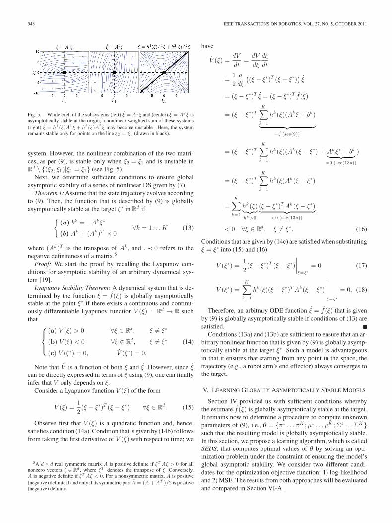
The eigenvalues of the two matrices A1 and A2 are complexwith values −1 ± 3.16i. Hence, each matrix determines a stable


Fig. 5. While each of the subsystems (left) ξ = A1 ξ and (center) ξ = A2 ξ isasymptotically stable at the origin, a nonlinear weighted sum of these systems(right) ξ = h1 (ξ)A1 ξ + h2 (ξ)A2 ξ may become unstable . Here, the systemremains stable only for points on the line ξ2 = ξ1 (drawn in black).

system. However, the nonlinear combination of the two matri-ces, as per (9), is stable only when ξ2 = ξ1 and is unstable inR

d \ {(ξ2 , ξ1)|ξ2 = ξ1} (see Fig. 5).Next, we determine sufficient conditions to ensure global

asymptotic stability of a series of nonlinear DS given by (7).Theorem 1: Assume that the state trajectory evolves according

to (9). Then, the function that is described by (9) is globallyasymptotically stable at the target ξ∗ in R

d if{(a) bk = −Akξ∗

(b) Ak + (Ak )T ≺ 0∀k = 1 . . . K (13)

where (Ak )T is the transpose of Ak , and . ≺ 0 refers to thenegative definiteness of a matrix.5

Proof: We start the proof by recalling the Lyapunov con-ditions for asymptotic stability of an arbitrary dynamical sys-tem [19].

Lyapunov Stability Theorem: A dynamical system that is de-termined by the function ξ = f(ξ) is globally asymptoticallystable at the point ξ∗ if there exists a continuous and continu-ously differentiable Lyapunov function V (ξ) : R

d → R suchthat ⎧⎪⎨

⎪⎩(a) V (ξ) > 0 ∀ξ ∈ R

d , ξ = ξ∗

(b) V (ξ) < 0 ∀ξ ∈ Rd , ξ = ξ∗

(c) V (ξ∗) = 0, V (ξ∗) = 0.

(14)

Note that V is a function of both ξ and ξ. However, since ξcan be directly expressed in terms of ξ using (9), one can finallyinfer that V only depends on ξ.

Consider a Lyapunov function V (ξ) of the form

V (ξ) =12(ξ − ξ∗)T (ξ − ξ∗) ∀ξ ∈ R

d . (15)

Observe first that V (ξ) is a quadratic function and, hence,satisfies condition (14a). Condition that is given by (14b) followsfrom taking the first derivative of V (ξ) with respect to time; we

5A d × d real symmetric matrix A is positive definite if ξT Aξ > 0 for allnonzero vectors ξ ∈ R

d , where ξT denotes the transpose of ξ. Conversely,A is negative definite if ξT Aξ < 0. For a nonsymmetric matrix, A is positive(negative) definite if and only if its symmetric part A = (A + AT )/2 is positive(negative) definite.

have

V (ξ) =dV

dt=

dV

dξ

dξ

dt

=12

d

dξ

((ξ − ξ∗)T (ξ − ξ∗)

)ξ

= (ξ − ξ∗)T ξ = (ξ − ξ∗)T f(ξ)

= (ξ − ξ∗)TK∑

k=1

hk (ξ)(Akξ + bk )

︸︷︷︸= ξ (see(9))

= (ξ − ξ∗)TK∑

k=1

hk (ξ)(Ak (ξ − ξ∗) + Akξ∗ + bk︸︷︷︸=0 (see(13a))

)

= (ξ − ξ∗)TK∑

k=1

hk (ξ)Ak (ξ − ξ∗)

=K∑

k=1

hk (ξ)︸︷︷︸hk >0

(ξ − ξ∗)T Ak (ξ − ξ∗)︸︷︷︸<0 (see(13b))

< 0 ∀ξ ∈ Rd , ξ = ξ∗. (16)

Conditions that are given by (14c) are satisfied when substitutingξ = ξ∗ into (15) and (16)

V (ξ∗) =12(ξ − ξ∗)T (ξ − ξ∗)

∣∣∣∣ξ=ξ ∗

= 0 (17)

V (ξ∗) =K∑

k=1

hk (ξ)(ξ − ξ∗)T Ak (ξ − ξ∗)

∣∣∣∣∣ξ=ξ ∗

= 0. (18)

Therefore, an arbitrary ODE function ξ = f(ξ) that is givenby (9) is globally asymptotically stable if conditions of (13) aresatisfied. �

Conditions (13a) and (13b) are sufficient to ensure that an ar-bitrary nonlinear function that is given by (9) is globally asymp-totically stable at the target ξ∗. Such a model is advantageousin that it ensures that starting from any point in the space, thetrajectory (e.g., a robot arm’s end effector) always converges tothe target.

V. LEARNING GLOBALLY ASYMPTOTICALLY STABLE MODELS

Section IV provided us with sufficient conditions wherebythe estimate f(ξ) is globally asymptotically stable at the target.It remains now to determine a procedure to compute unknownparameters of (9), i.e., θ = {π1 . . . πK ;μ1 . . . μK ; Σ1 . . . ΣK }such that the resulting model is globally asymptotically stable.In this section, we propose a learning algorithm, which is calledSEDS, that computes optimal values of θ by solving an opti-mization problem under the constraint of ensuring the model’sglobal asymptotic stability. We consider two different candi-dates for the optimization objective function: 1) log-likelihoodand 2) MSE. The results from both approaches will be evaluatedand compared in Section VI-A.


SEDS-Likelihood: Using log-likelihood as a means to con-struct a model

minθ

J(θ) = − 1T

N∑n=1

T n∑t=0

logP(ξt,n , ξt,n |θ) (19)

subject to

⎧⎪⎪⎪⎪⎪⎪⎪⎨⎪⎪⎪⎪⎪⎪⎪⎩

(a) bk = −Akξ∗

(b) Ak + (Ak )T ≺ 0

(c) Σk � 0

(d) 0 < πk ≤ 1

(e)∑K

k=1 πk = 1

∀k ∈ 1 . . . K (20)

where P(ξt,n , ξt,n |θ) is given by (5), and T =∑N

n=1 Tn is thetotal number of training data points. The first two constraintsin (20) are stability conditions from Section IV. The last threeconstraints are imposed by the nature of the Gaussian mixturemodel to ensure that Σk are positive-definite matrices, priorsπk are positive scalars smaller than or equal to one, and sum ofall priors is equal to one (because the probability value of (5)should not exceed 1).

SEDS-MSE: Using MSE as a means to quantify the accuracyof estimations that are based on demonstrations6

minθ

J(θ) =1

2T

N∑n=1

T n∑t=0

‖ ˆξt,n − ξt,n‖2 (21)

subject to the same constraints as given by (20). In (21), ˆξt,n =

f(ξt,n ) are computed directly from (9).Both SEDS-Likelihood and SEDS-MSE can be formulated

as a Nonlinear Programming (NLP) problem [32] and can besolved using standard constrained optimization techniques. Weuse a Successive Quadratic Programming (SQP) approach thatrelies on a quasi-Newton method7 to solve the constrained opti-mization problem [32]. SQP minimizes a quadratic approxima-tion of the Lagrangian function over a linear approximation ofthe constraints.8

Our implementation of SQP has several advantages over gen-eral purpose solvers. First, we have an analytic expression of

6In our previous work [5], we used a different MSE cost function, whichbalanced the effect of following the trajectory and the speed. See Appendix Afor a comparison of results using both cost functions and further discussion.

7Quasi-Newton methods differ from classical Newton methods in that theycompute an estimate of the Hessian function H (ξ) and, thus, do not require auser to provide it explicitly. The estimate of the Hessian function progressivelyapproaches to its real value as optimization proceeds. Among quasi-Newtonmethods, we use Broyden–Fletcher–Goldfard–Shanno [32].

8Given the derivative of the constraints and an estimate of the Hessian andthe derivatives of the cost function with respect to the optimization parameters,the SQP method finds a proper descent direction (if it exists) that minimizes thecost function while not violating the constraints. To satisfy equality constraints,SQP finds a descent direction that minimizes the cost function by varyingthe parameters on the hypersurface that satisfies the equality constraints. Forinequality constraints, SQP follows the gradient direction of the cost functionwhenever the inequality holds (inactive constraints). Only at the hypersurfacewhere the inequality constraint becomes active does SQP look for a descentdirection that minimizes the cost function by varying the parameters on thehypersurface or toward the inactive constraint domain.

the derivatives, improving significantly the performances. Sec-ond, our code is tailored to solve the specific problem at hand.For example, a reformulation guarantees that the optimizationconstraints (20a), (20c), (20d), and (20e) are satisfied. Thereis, thus, no longer the need to explicitly enforce them duringthe optimization. The analytical formulation of derivatives andthe mathematical reformulation to satisfy the optimization con-straints are explained in detail in [33].

Note that a feasible solution to these NLP problems alwaysexists. Algorithm 1 provides a simple and efficient way to com-pute a feasible initial guess for the optimization parameters.Starting from an initial value, the solver tries to optimize thevalue of θ such that the cost function J is minimized. How-ever, since the proposed NLP problem is nonconvex, one cannotensure to find the globally optimal solution. Solvers are usu-ally very sensitive to initialization of the parameters and willoften converge to some local minima of the objective function.Based on our experiments, running the optimization with theinitial guess that is obtained from Algorithm 1 usually results ina good local minimum. In all experiments that are reported inSection VI, we ran the initialization three to four times, and usethe result from the best run for the performance analysis.

We use the BIC to choose the optimal set K of Gaussians.The BIC determines a tradeoff between optimizing the model’slikelihood and the number of parameters that are needed toencode the data

BIC = T J(θ) +np

2log(T ) (22)

where J(θ) is the normalized log-likelihood of the model thatis computed using (19), and np is the total number of freeparameters. The SEDS-Likelihood approach requires the esti-mation of K(1 + 3d + 2d2) parameters (the priors πk , meanμk , and covariance Σk are of size 1, 2d, and d(2d + 1),


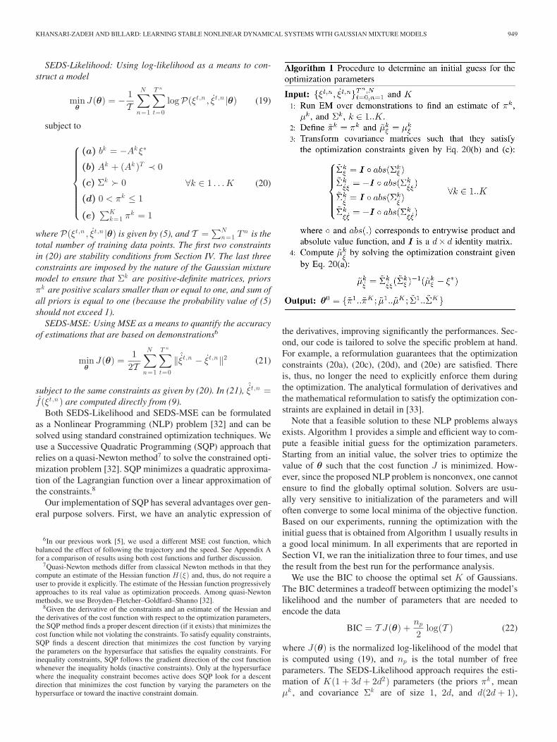
Fig. 6. Performance comparison of SEDS-Likelihood and SEDS-MSE through a library of 20 human handwriting motions.

respectively). However, the number of parameters can be re-duced since the constraints given by (20a) provide an explicitformulation to compute μk

ξfrom other parameters (i.e., μk

ξ , Σkξ ,

and Σkξξ

). Thus, the total number of parameters to construct a

GMM with K Gaussians is K(1 + 2d(d + 1)). As for SEDS-MSE, the number of parameters is even more reduced sincewhen constructing f , the term Σk

ξis not used and, thus, can be

omitted during the optimization. Taking this into account, thetotal number of learning parameters for the SEDS-MSE reducesto K(1 + 3

2 d(d + 1)). For both approaches, learning grows lin-early with the number of Gaussians and quadratically with thedimension. In comparison, the number of parameters in the pro-posed method is fewer than GMM and LWPR.9 The retrievaltime of the proposed method is low and in the same order ofGMR and LWPR.

The source code of SEDS can be downloaded fromhttp://lasa.epfl.ch/sourcecode/.

VI. EXPERIMENTAL EVALUATIONS

Performance of the proposed method is first evaluated againsta library of 20 human handwriting motions. These were chosenas they provide realistic human motions while ensuring thatimprecision in both recording and generating motion is minimal.Precisely, in Section VI-A, we compare the performance ofthe SEDS method when using either the likelihood or MSE.In Section VI-B, we validate SEDS to estimate the dynamicsof motion of two robot platforms: 1) the 7-DOF right arm of

9The number of learning parameter in GMR and LWPR is K (1 + 3d + 2d2 )and 7

2 K (d + d2 ), respectively.

the humanoid robot iCub and 2) the six DOF industrial robotKatana-T arm. In Sections VI-C and VI-D, we show that themethod can learn second- and higher order dynamics that allowsus to embed different local dynamics in the same model. Finally,in Section VI-E, we compare our method with those of fouralternative methods GMR, LWPR, GPR, and BM.

A. Stable Estimator of Dynamical Systems: Likelihood VersusMean Square Error

In Section V, we proposed two objective functions: likelihoodand MSE for training the SEDS model. We compare the resultsthat are obtained with each method for modeling 20 handwritingmotions. The demonstrations are collected from pen input usinga Tablet-PC. Fig. 6 shows a qualitative comparison of the esti-mate of handwriting motions. All reproductions were generatedin simulation to exclude the error due to the robot controllerfrom the modeling error. The accuracy of the estimate is mea-sured according to (23), with which the method accuracy inestimating the overall dynamics of the underlying model f isquantified by measuring the discrepancy between the directionand magnitude of the estimated and observed velocity vectorsfor all training data points10

10Equation (23) measures the error in our estimation of both the directionand magnitude of the velocity. It is, hence, a better estimate of how well ourmodel encapsulates the dynamics of the motion, in contrast with an MSE on thevelocity magnitude alone.


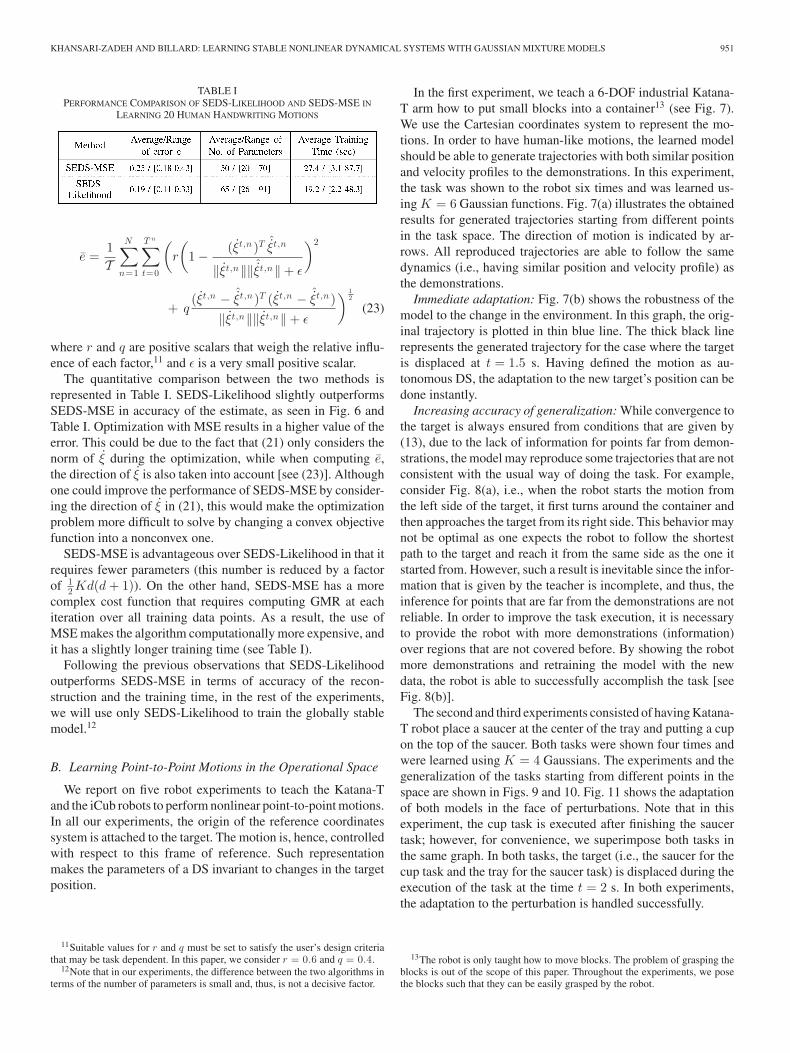
TABLE IPERFORMANCE COMPARISON OF SEDS-LIKELIHOOD AND SEDS-MSE IN

LEARNING 20 HUMAN HANDWRITING MOTIONS

e =1T

N∑n=1

T n∑t=0

(r

(1 − (ξt,n )T ˆ

ξt,n

‖ξt,n‖‖ ˆξt,n‖ + ε

)2

+ q(ξt,n − ˆ

ξt,n )T (ξt,n − ˆξt,n )

‖ξt,n‖‖ξt,n‖ + ε

) 12

(23)

where r and q are positive scalars that weigh the relative influ-ence of each factor,11 and ε is a very small positive scalar.

The quantitative comparison between the two methods isrepresented in Table I. SEDS-Likelihood slightly outperformsSEDS-MSE in accuracy of the estimate, as seen in Fig. 6 andTable I. Optimization with MSE results in a higher value of theerror. This could be due to the fact that (21) only considers thenorm of ξ during the optimization, while when computing e,the direction of ξ is also taken into account [see (23)]. Althoughone could improve the performance of SEDS-MSE by consider-ing the direction of ξ in (21), this would make the optimizationproblem more difficult to solve by changing a convex objectivefunction into a nonconvex one.

SEDS-MSE is advantageous over SEDS-Likelihood in that itrequires fewer parameters (this number is reduced by a factorof 1

2 Kd(d + 1)). On the other hand, SEDS-MSE has a morecomplex cost function that requires computing GMR at eachiteration over all training data points. As a result, the use ofMSE makes the algorithm computationally more expensive, andit has a slightly longer training time (see Table I).

Following the previous observations that SEDS-Likelihoodoutperforms SEDS-MSE in terms of accuracy of the recon-struction and the training time, in the rest of the experiments,we will use only SEDS-Likelihood to train the globally stablemodel.12

B. Learning Point-to-Point Motions in the Operational Space

We report on five robot experiments to teach the Katana-Tand the iCub robots to perform nonlinear point-to-point motions.In all our experiments, the origin of the reference coordinatessystem is attached to the target. The motion is, hence, controlledwith respect to this frame of reference. Such representationmakes the parameters of a DS invariant to changes in the targetposition.

11Suitable values for r and q must be set to satisfy the user’s design criteriathat may be task dependent. In this paper, we consider r = 0.6 and q = 0.4.

12Note that in our experiments, the difference between the two algorithms interms of the number of parameters is small and, thus, is not a decisive factor.

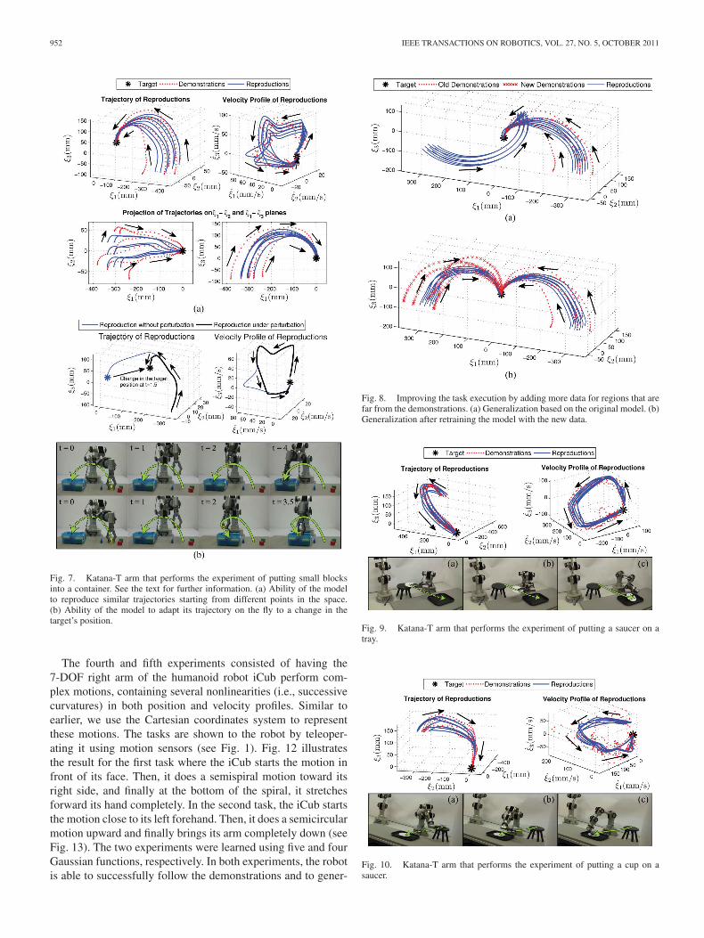
In the first experiment, we teach a 6-DOF industrial Katana-T arm how to put small blocks into a container13 (see Fig. 7).We use the Cartesian coordinates system to represent the mo-tions. In order to have human-like motions, the learned modelshould be able to generate trajectories with both similar positionand velocity profiles to the demonstrations. In this experiment,the task was shown to the robot six times and was learned us-ing K = 6 Gaussian functions. Fig. 7(a) illustrates the obtainedresults for generated trajectories starting from different pointsin the task space. The direction of motion is indicated by ar-rows. All reproduced trajectories are able to follow the samedynamics (i.e., having similar position and velocity profile) asthe demonstrations.

Immediate adaptation: Fig. 7(b) shows the robustness of themodel to the change in the environment. In this graph, the orig-inal trajectory is plotted in thin blue line. The thick black linerepresents the generated trajectory for the case where the targetis displaced at t = 1.5 s. Having defined the motion as au-tonomous DS, the adaptation to the new target’s position can bedone instantly.

Increasing accuracy of generalization: While convergence tothe target is always ensured from conditions that are given by(13), due to the lack of information for points far from demon-strations, the model may reproduce some trajectories that are notconsistent with the usual way of doing the task. For example,consider Fig. 8(a), i.e., when the robot starts the motion fromthe left side of the target, it first turns around the container andthen approaches the target from its right side. This behavior maynot be optimal as one expects the robot to follow the shortestpath to the target and reach it from the same side as the one itstarted from. However, such a result is inevitable since the infor-mation that is given by the teacher is incomplete, and thus, theinference for points that are far from the demonstrations are notreliable. In order to improve the task execution, it is necessaryto provide the robot with more demonstrations (information)over regions that are not covered before. By showing the robotmore demonstrations and retraining the model with the newdata, the robot is able to successfully accomplish the task [seeFig. 8(b)].

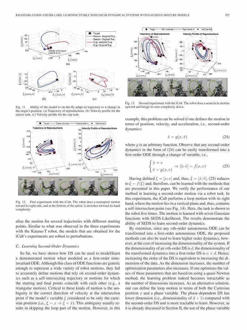
The second and third experiments consisted of having Katana-T robot place a saucer at the center of the tray and putting a cupon the top of the saucer. Both tasks were shown four times andwere learned using K = 4 Gaussians. The experiments and thegeneralization of the tasks starting from different points in thespace are shown in Figs. 9 and 10. Fig. 11 shows the adaptationof both models in the face of perturbations. Note that in thisexperiment, the cup task is executed after finishing the saucertask; however, for convenience, we superimpose both tasks inthe same graph. In both tasks, the target (i.e., the saucer for thecup task and the tray for the saucer task) is displaced during theexecution of the task at the time t = 2 s. In both experiments,the adaptation to the perturbation is handled successfully.

13The robot is only taught how to move blocks. The problem of grasping theblocks is out of the scope of this paper. Throughout the experiments, we posethe blocks such that they can be easily grasped by the robot.


Fig. 7. Katana-T arm that performs the experiment of putting small blocksinto a container. See the text for further information. (a) Ability of the modelto reproduce similar trajectories starting from different points in the space.(b) Ability of the model to adapt its trajectory on the fly to a change in thetarget’s position.

The fourth and fifth experiments consisted of having the7-DOF right arm of the humanoid robot iCub perform com-plex motions, containing several nonlinearities (i.e., successivecurvatures) in both position and velocity profiles. Similar toearlier, we use the Cartesian coordinates system to representthese motions. The tasks are shown to the robot by teleoper-ating it using motion sensors (see Fig. 1). Fig. 12 illustratesthe result for the first task where the iCub starts the motion infront of its face. Then, it does a semispiral motion toward itsright side, and finally at the bottom of the spiral, it stretchesforward its hand completely. In the second task, the iCub startsthe motion close to its left forehand. Then, it does a semicircularmotion upward and finally brings its arm completely down (seeFig. 13). The two experiments were learned using five and fourGaussian functions, respectively. In both experiments, the robotis able to successfully follow the demonstrations and to gener-

Fig. 8. Improving the task execution by adding more data for regions that arefar from the demonstrations. (a) Generalization based on the original model. (b)Generalization after retraining the model with the new data.

Fig. 9. Katana-T arm that performs the experiment of putting a saucer on atray.

Fig. 10. Katana-T arm that performs the experiment of putting a cup on asaucer.


Fig. 11. Ability of the model to on-the-fly adapt its trajectory to a change inthe target’s position. (a) Trajectory of reproductions. (b) Velocity profile for thesaucer task. (c) Velocity profile for the cup task.

Fig. 12. First experiment with the iCub. The robot does a semispiral motiontoward its right side, and at the bottom of the spiral, it stretches forward its handcompletely.

alize the motion for several trajectories with different startingpoints. Similar to what was observed in the three experimentswith the Katana-T robot, the models that are obtained for theiCub’s experiments are robust to perturbations.

C. Learning Second-Order Dynamics

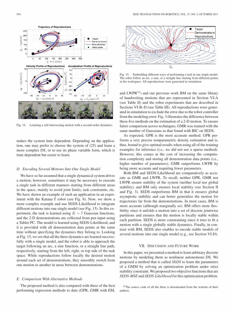
So far, we have shown how DS can be used to model/learna demonstrated motion when modeled as a first-order time-invariant ODE. Although this class of ODE functions are genericenough to represent a wide variety of robot motions, they failto accurately define motions that rely on second-order dynam-ics such as a self-intersecting trajectory or motions for whichthe starting and final points coincide with each other (e.g., atriangular motion). Critical to these kinds of motion is the am-biguity in the correct direction of velocity at the intersectionpoint if the model’s variable ξ considered to be only the carte-sian position (i.e., ξ = x ⇒ ξ = x). This ambiguity usually re-sults in skipping the loop part of the motion. However, in this

Fig. 13. Second experiment with the iCub. The robot does a semicircle motionupward and brings its arm completely down.

example, this problem can be solved if one defines the motion interms of position, velocity, and acceleration, i.e., second-orderdynamics:

x = g(x, x) (24)

where g is an arbitrary function. Observe that any second-orderdynamics in the form of (24) can be easily transformed into afirst-order ODE through a change of variable, i.e.,{

x = v

v = g(x, v)⇒ [x; v] = f(x, v) (25)

Having defined ξ = [x; v] and, thus, ξ = [x; v], (25) reducesto ξ = f(ξ) and, therefore, can be learned with the methods thatare presented in this paper. We verify the performance of ourmethod in learning a second-order motion via a robot task. Inthis experiment, the iCub performs a loop motion with its righthand, where the motion lies in a vertical plane and, thus, containsa self-intersection point (see Fig. 14). Here, the task is shown tothe robot five times. The motion is learned with seven Gaussianfunctions with SEDS-Likelihood. The results demonstrate theability of SEDS to learn second-order dynamics.

By extension, since any nth-order autonomous ODE can betransformed into a first-order autonomous ODE, the proposedmethods can also be used to learn higher order dynamics, how-ever, at the cost of increasing the dimensionality of the system. Ifthe dimensionality of an nth-order DS is d, the dimensionality ofthe transformed dynamics into a first-order DS is n × d. Hence,increasing the order of the DS is equivalent to increasing the di-mension of the data. As the dimension increases, the number ofoptimization parameters also increases. If one optimizes the val-ues of these parameters that are based on using a quasi-Newtonmethod, the learning problem indeed becomes intractable asthe number of dimensions increases. As an alternative solution,one can define the loop motion in terms of both the Cartesianposition x and a phase variable. The phase-dependent DS haslower dimension (i.e., dimensionality of d + 1) compared withthe second-order DS and is more tractable to learn. However, asit is already discussed in Section II, the use of the phase variable


Fig. 14. Learning a self-intersecting motion with a second-order dynamics.

makes the system time dependent. Depending on the applica-tion, one may prefer to choose the system of (25) and learn amore complex DS, or to use its phase variable form, which istime dependent but easier to learn.

D. Encoding Several Motions Into One Single Model

We have so far assumed that a single dynamical system drivesa motion; however, sometimes it may be necessary to executea single task in different manners starting from different areasin the space, mainly to avoid joint limits, task constraints, etc.We have shown an example of such an application in an exper-iment with the Katana-T robot (see Fig. 8). Now, we show amore complex example and use SEDS-Likelihood to integratedifferent motions into one single model (see Fig. 15). In this ex-periment, the task is learned using K = 7 Gaussian functions,and the 2-D demonstrations are collected from pen input usinga Tablet-PC. The model is learned using SEDS-Likelihood, andit is provided with all demonstration data points at the sametime without specifying the dynamics they belong to. Lookingat Fig. 15, we see that all the three dynamics are learned success-fully with a single model, and the robot is able to approach thetarget following an arc, a sine function, or a straight line path,respectively, starting from the left, right, or top side of the taskspace. While reproductions follow locally the desired motionaround each set of demonstrations, they smoothly switch fromone motion to another in areas between demonstrations.

E. Comparison With Alternative Methods

The proposed method is also compared with three of the bestperforming regression methods to date (GPR, GMR with EM,

Fig. 15. Embedding different ways of performing a task in one single model.The robot follow an arc, a sine, or a straight line starting from different pointsin the workspace. All reproductions were generated in simulation.

and LWPR14) and our previous work BM on the same libraryof handwriting motions that are represented in Section VI-A(see Table II) and the robot experiments that are described inSections VI-B–D (see Table III). All reproductions were gener-ated in simulation to exclude the error due to the robot controllerfrom the modeling error. Fig. 3 illustrates the difference betweenthese five methods on the estimation of a 2-D motion. To ensurefairer comparison across techniques, GMR was trained with thesame number of Gaussians as that found with BIC on SEDS.

As expected, GPR is the most accurate method. GPR per-forms a very precise nonparametric density estimation and is,thus, bound to give optimal results when using all of the trainingexamples for inference (i.e., we did not use a sparse method).However, this comes at the cost of increasing the computa-tion complexity and storing all demonstration data points (i.e.,higher number of parameters). GMR outperforms LWPR bybeing more accurate and requiring fewer parameters.

Both BM and SEDS-Likelihood are comparatively as accu-rate as GMR and LWPR. To recall, neither GPR, GMR norLWPR ensure stability of the system (neither local nor globalstability), and BM only ensures local stability (see Section IIand Fig. 3). SEDS outperforms BM in that it ensures globalasymptotic stability and can better generalize the motion fortrajectories far from the demonstrations. In most cases, BM ismore accurate (although marginally so). BM offers more flex-ibility since it unfolds a motion into a set of discrete jointwisepartitions and ensures that the motion is locally stable withineach partition. SEDS is more constraining since it tries to fit amotion with a single globally stable dynamics. Finally, in con-trast with BM, SEDS also enables to encode stable models ofseveral motions into one single model (e.g., see Section VI-D).

VII. DISCUSSION AND FUTURE WORK

In this paper, we presented a method to learn arbitrary discretemotions by modeling them as nonlinear autonomous DS. Weproposed a method that is called SEDS to learn the parametersof a GMM by solving an optimization problem under strictstability constraint. We proposed two objective functions that areSEDS-MSE and SEDS-Likelihood for this optimization problem.

14The source code of all the three is downloaded from the website of theirauthors.


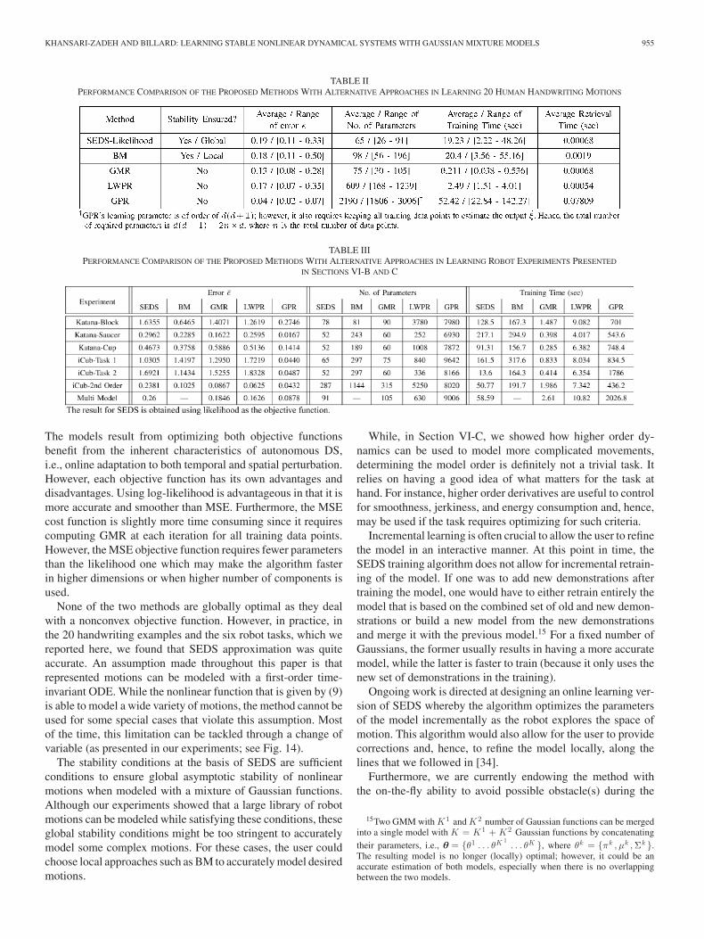
TABLE IIPERFORMANCE COMPARISON OF THE PROPOSED METHODS WITH ALTERNATIVE APPROACHES IN LEARNING 20 HUMAN HANDWRITING MOTIONS

TABLE IIIPERFORMANCE COMPARISON OF THE PROPOSED METHODS WITH ALTERNATIVE APPROACHES IN LEARNING ROBOT EXPERIMENTS PRESENTED

IN SECTIONS VI-B AND C

The models result from optimizing both objective functionsbenefit from the inherent characteristics of autonomous DS,i.e., online adaptation to both temporal and spatial perturbation.However, each objective function has its own advantages anddisadvantages. Using log-likelihood is advantageous in that it ismore accurate and smoother than MSE. Furthermore, the MSEcost function is slightly more time consuming since it requirescomputing GMR at each iteration for all training data points.However, the MSE objective function requires fewer parametersthan the likelihood one which may make the algorithm fasterin higher dimensions or when higher number of components isused.

None of the two methods are globally optimal as they dealwith a nonconvex objective function. However, in practice, inthe 20 handwriting examples and the six robot tasks, which wereported here, we found that SEDS approximation was quiteaccurate. An assumption made throughout this paper is thatrepresented motions can be modeled with a first-order time-invariant ODE. While the nonlinear function that is given by (9)is able to model a wide variety of motions, the method cannot beused for some special cases that violate this assumption. Mostof the time, this limitation can be tackled through a change ofvariable (as presented in our experiments; see Fig. 14).

The stability conditions at the basis of SEDS are sufficientconditions to ensure global asymptotic stability of nonlinearmotions when modeled with a mixture of Gaussian functions.Although our experiments showed that a large library of robotmotions can be modeled while satisfying these conditions, theseglobal stability conditions might be too stringent to accuratelymodel some complex motions. For these cases, the user couldchoose local approaches such as BM to accurately model desiredmotions.

While, in Section VI-C, we showed how higher order dy-namics can be used to model more complicated movements,determining the model order is definitely not a trivial task. Itrelies on having a good idea of what matters for the task athand. For instance, higher order derivatives are useful to controlfor smoothness, jerkiness, and energy consumption and, hence,may be used if the task requires optimizing for such criteria.

Incremental learning is often crucial to allow the user to refinethe model in an interactive manner. At this point in time, theSEDS training algorithm does not allow for incremental retrain-ing of the model. If one was to add new demonstrations aftertraining the model, one would have to either retrain entirely themodel that is based on the combined set of old and new demon-strations or build a new model from the new demonstrationsand merge it with the previous model.15 For a fixed number ofGaussians, the former usually results in having a more accuratemodel, while the latter is faster to train (because it only uses thenew set of demonstrations in the training).

Ongoing work is directed at designing an online learning ver-sion of SEDS whereby the algorithm optimizes the parametersof the model incrementally as the robot explores the space ofmotion. This algorithm would also allow for the user to providecorrections and, hence, to refine the model locally, along thelines that we followed in [34].

Furthermore, we are currently endowing the method withthe on-the-fly ability to avoid possible obstacle(s) during the

15Two GMM with K 1 and K 2 number of Gaussian functions can be mergedinto a single model with K = K 1 + K 2 Gaussian functions by concatenatingtheir parameters, i.e., θ = {θ1 . . . θK 1

. . . θK }, where θk = {πk , μk , Σk }.The resulting model is no longer (locally) optimal; however, it could be anaccurate estimation of both models, especially when there is no overlappingbetween the two models.


execution of a task. We will also focus on integrating physicalconstraints of the system (e.g., robot’s joints limit, the task’sconstraint, etc.) into the model to solve for this during our globaloptimization. Finally, while we have shown that the systemcould embed more than one motion and, hence, account fordifferent ways to approach the same target, depending on wherethe motion starts in the workspace, we have still yet to determinehow many different dynamics can be embedded in the samesystem.

VIII. SUMMARY

DS offer a framework that allows for fast learning of robotmotions from a small set of demonstrations. They are also ad-vantageous in that they can be easily modulated to producetrajectories with similar dynamics in areas of the workspacethat is not covered during training. However, their applicationto robot control has been given little attention so far, mainlybecause of the difficulty of ensuring stability. In this paper, wepresented an optimization approach for statistically encoding adynamical motion as a first-order autonomous nonlinear ODEwith Gaussian Mixtures. We addressed the stability problem ofautonomous nonlinear DS and formulated sufficient conditionsto ensure global asymptotic stability of such a system. Then,we proposed two optimization problems to construct a globallystable estimate of a motion from demonstrations.

We compared performance of the proposed method with cur-rent widely used regression techniques via a library of 20 hand-writing motions. Furthermore, we validated the methods in dif-ferent point-to-point robot tasks that are performed with twodifferent robots. In all experiments, the proposed method wasable to successfully accomplish the experiments in terms of highaccuracy during reproduction, the ability to generalize motionsto unseen contexts, and the ability to adapt on the fly to spatialand temporal perturbations.

APPENDIX A

COMPARISON WITH THE COST FUNCTION DESCRIBED IN [5]

In our previous work [5], we had used a different MSE costfunction from that proposed in this paper that balanced the errorin both position and velocity

minθ

J(θ) =1N

N∑n=1

T n∑t=0

(ωξ‖ξn (t) − ξt,n‖2

+ ωξ‖ˆξn (t) − ξt,n‖2

). (26)

ˆξn (t) = f(ξn (t)) are computed directly from (9). ξn (t) =∑t

i=0ˆξn (i)dt generate an estimate of the corresponding demon-

strated trajectory ξn by starting from the same initial points asthat demonstrated, i.e., ξn (0) = ξ0,n ∀n ∈ 1 . . . N . ωξ and ωξ

are positive scalars weighing the influence of the position andvelocity terms in the cost function.

In contrast with the cost function that is proposed in this pa-per that assumes independence across data points [see (21)], theaforementioned cost function propagates the effect of the esti-

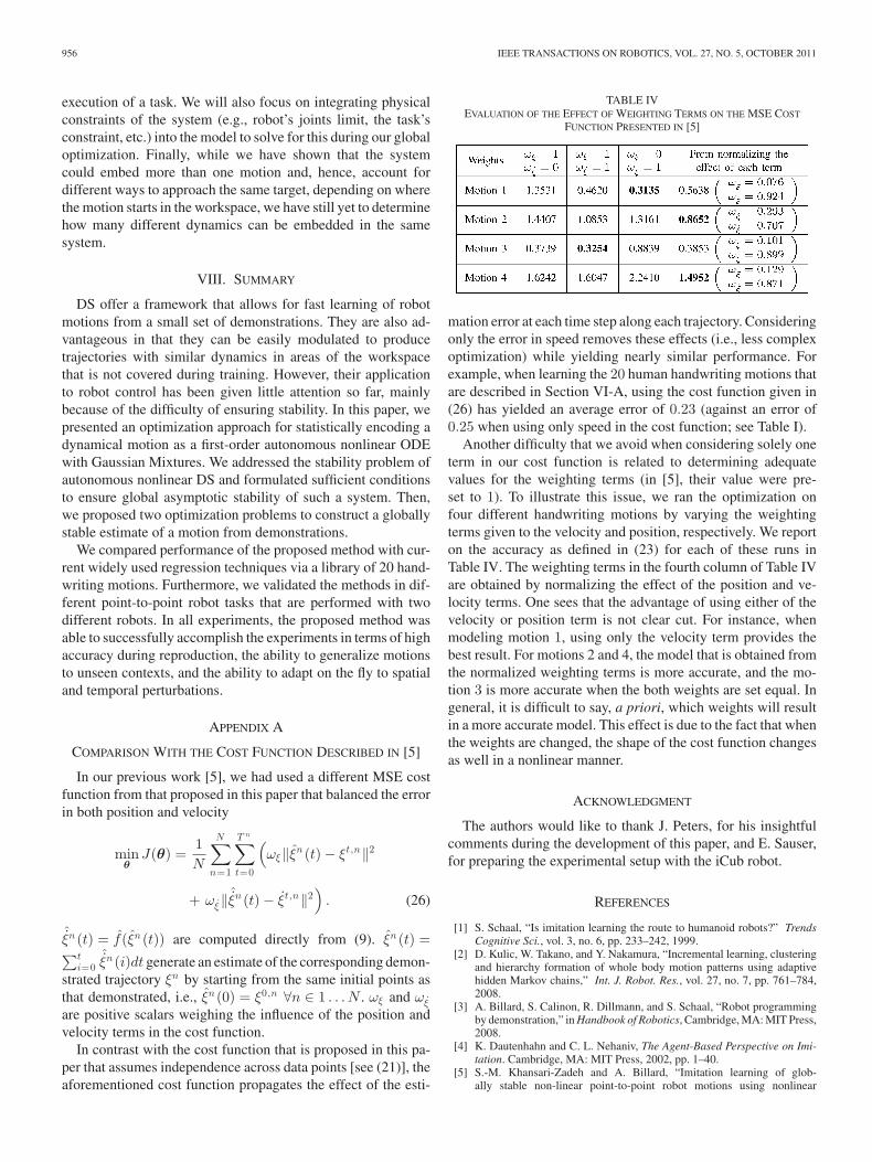
TABLE IVEVALUATION OF THE EFFECT OF WEIGHTING TERMS ON THE MSE COST

FUNCTION PRESENTED IN [5]

mation error at each time step along each trajectory. Consideringonly the error in speed removes these effects (i.e., less complexoptimization) while yielding nearly similar performance. Forexample, when learning the 20 human handwriting motions thatare described in Section VI-A, using the cost function given in(26) has yielded an average error of 0.23 (against an error of0.25 when using only speed in the cost function; see Table I).

Another difficulty that we avoid when considering solely oneterm in our cost function is related to determining adequatevalues for the weighting terms (in [5], their value were pre-set to 1). To illustrate this issue, we ran the optimization onfour different handwriting motions by varying the weightingterms given to the velocity and position, respectively. We reporton the accuracy as defined in (23) for each of these runs inTable IV. The weighting terms in the fourth column of Table IVare obtained by normalizing the effect of the position and ve-locity terms. One sees that the advantage of using either of thevelocity or position term is not clear cut. For instance, whenmodeling motion 1, using only the velocity term provides thebest result. For motions 2 and 4, the model that is obtained fromthe normalized weighting terms is more accurate, and the mo-tion 3 is more accurate when the both weights are set equal. Ingeneral, it is difficult to say, a priori, which weights will resultin a more accurate model. This effect is due to the fact that whenthe weights are changed, the shape of the cost function changesas well in a nonlinear manner.

ACKNOWLEDGMENT

The authors would like to thank J. Peters, for his insightfulcomments during the development of this paper, and E. Sauser,for preparing the experimental setup with the iCub robot.

REFERENCES

[1] S. Schaal, “Is imitation learning the route to humanoid robots?” TrendsCognitive Sci., vol. 3, no. 6, pp. 233–242, 1999.

[2] D. Kulic, W. Takano, and Y. Nakamura, “Incremental learning, clusteringand hierarchy formation of whole body motion patterns using adaptivehidden Markov chains,” Int. J. Robot. Res., vol. 27, no. 7, pp. 761–784,2008.

[3] A. Billard, S. Calinon, R. Dillmann, and S. Schaal, “Robot programmingby demonstration,” in Handbook of Robotics, Cambridge, MA: MIT Press,2008.

[4] K. Dautenhahn and C. L. Nehaniv, The Agent-Based Perspective on Imi-tation. Cambridge, MA: MIT Press, 2002, pp. 1–40.

[5] S.-M. Khansari-Zadeh and A. Billard, “Imitation learning of glob-ally stable non-linear point-to-point robot motions using nonlinear


programming,” in Proc. IEEE/RSJ Int. Conf. Intell. Robots Syst., 2010,pp. 2676–2683.

[6] E. D. Sontag, “Input to state stability: Basic concepts and results,” inNonlinear and Optimal Control Theory, Berlin/Heidelberg, Germany:Springer-Verlag, 2008, ch. 3, pp. 163–220.

[7] J.-H. Hwang, R. Arkin, and D.-S. Kwon, “Mobile robots at your fingertip:Bezier curve on-line trajectory generation for supervisory control,” inProc. IEEE/RSJ Int. Conf. Intell. Robots Syst., vol. 2, 2003, pp. 1444–1449.

[8] R. Andersson, “Aggressive trajectory generator for a robot ping-pongplayer,” IEEE Control Syst. Mag., vol. 9, no. 2, pp. 15–21, Feb. 1989.

[9] J. Aleotti and S. Caselli, “Robust trajectory learning and approximationfor robot programming by demonstration,” Robot. Auton. Syst., vol. 54,pp. 409–413, 2006.

[10] A. Ude, “Trajectory generation from noisy positions of object features forteaching robot paths,” Robot. Auton. Syst., vol. 11, no. 2, pp. 113–127,1993.

[11] M. Muehlig, M. Gienger, S. Hellbach, J. Steil, and C. Goerick, “Task levelimitation learning using variance-based movement optimization,” in Proc.IEEE Int. Conf. Robot. Autom., 2009, pp. 1177–1184.

[12] K. Yamane, J. J. Kuffner, and J. K. Hodgins, “Synthesizing animations ofhuman manipulation tasks,” ACM Trans. Graph., vol. 23, no. 3, pp. 532–539, 2007.

[13] A. Coates, P. Abbeel, and A. Y. Ng, “Learning for control from multipledemonstrations,” in Proc. 25th Int. Conf. Mach. Learning, 2008, pp. 144–151.

[14] M. Hersch, F. Guenter, S. Calinon, and A. Billard, “Dynamical systemmodulation for robot learning via kinesthetic demonstrations,” IEEETrans. Robot., vol. 24, no. 6, pp. 1463–1467, Dec. 2008.

[15] C. Rasmussen and C. Williams, Gaussian Processes for Machine Learn-ing. New York: Springer-Verlag, 2006.

[16] S. Schaal, C. Atkeson, and S. Vijayakumar, “Scalable locally weightedstatistical techniques for real time robot learning,” Appl. Intell.—Spec.Issue Scalable Robot. Appl. Neural Netw., vol. 17, no. 1, pp. 49–60, 2002.

[17] A. Dempster and N. L. D. Rubin, “Maximum likelihood from incompletedata via the EM algorithm,” J. R. Statist. Soc. B, vol. 39, no. 1, pp. 1–38,1977.

[18] S.-M. Khansari-Zadeh and A. Billard, “BM: An iterative algorithm to learnstable non-linear dynamical systems with Gaussian Mixture Models,” inProc. Int. Conf. Robot. Autom., 2010, pp. 2381–2388.

[19] J. Slotine and W. Li, Applied Nonlinear Control. Englewood Cliffs, NJ:Prentice-Hall, 1991.

[20] P. Pastor, H. Hoffmann, T. Asfour, and S. Schaal, “Learning and gener-alization of motor skills by learning from demonstration,” in Proc. Int.Conf. Robot. Autom., 2009, pp. 1293–1298.

[21] E. Gribovskaya, S. M. Khansari-Zadeh, and A. Billard, “Learning non-linear multivariate dynamics of motion in robotic manipulators,” Int. J.Robot. Res., vol. 30, pp. 1–37, 2010.

[22] S. Calinon, F. D’halluin, E. Sauser, D. Caldwell, and A. Billard, “Learningand reproduction of gestures by imitation: An approach based on hiddenMarkov model and Gaussian mixture regression,” IEEE Robot. Autom.Mag., vol. 17, no. 2, pp. 44–54, Jun. 2010.

[23] E. Gribovskaya and A. Billard, “Learning nonlinear multi-variate motiondynamics for real-time position and orientation control of robotic ma-nipulators,” in Proc. 9th IEEE-RAS Int. Conf. Humanoid Robots, 2009,pp. 472–477.

[24] G. McLachlan and D. Peel, Finite Mixture Models. New York: Wiley,2000.

[25] G. Schwarz, “Estimating the dimension of a model,” Ann. Statist., vol. 6,pp. 461–464, 1978.

[26] H. Akaike, “A new look at the statistical model identification,” IEEETrans. Automat. Control, vol. AC-19, no. 6, pp. 716–723, Dec. 1974.

[27] D. J. Spiegelhalter, N. G. Best, B. P. Carlin, and A. van der Linde,“Bayesian measures of model complexity and fit,” J. R. Statist. Soc.,Series B (Statist. Methodol.), vol. 64, pp. 583–639, 2002.

[28] D. Nguyen-Tuong, M. Seeger, and J. Peters, “Local Gaussian processregression for real time online model learning and control,” in Proc. Adv.Neural Inf. Process. Syst. 21, 2009, pp. 1193–1200.

[29] E. Snelson and Z. Ghahramani, “Sparse Gaussian processes using pseudo-inputs,” in Proc. Adv. Neural Inf. Process. Syst. 18, 2006, pp. 1257–1264.

[30] M. Seeger, C. K. I. Williams, and N. D. Lawrence, “Fast forward selec-tion to speed up sparse Gaussian Process Regression,” in Proc. 9th Int.Workshop Artif. Intell. Statist., 2003.

[31] D. Cohn and Z. Ghahramani, “Active learning with statistical models,”Artif. Intell. Res., vol. 4, pp. 129–145, 1996.

[32] M. S. Bazaraa, H. Sherali, and C. Shetty, Nonlinear Programming: Theoryand Algorithms, 3rd ed. New York: Wiley, 2006.

[33] S.-M. Khansari-Zadeh and A. Billard. (2010). “The derivativesof the SEDS optimization cost function and constraints with re-spect to its optimization parameters,” Ecole Polytech. Fed. Lau-sanne, Lausanne, Switzerland, Tech. Rep., [Online]. Available:http://lasa.epfl.ch/publications/publications.php

[34] B. D. Argall, E. Sauser, and A. Billard, “Tactile guidance for policyrefinement and reuse,” in Proc. 9th IEEE Int. Conf. Development Learning,2010, pp. 7–12.

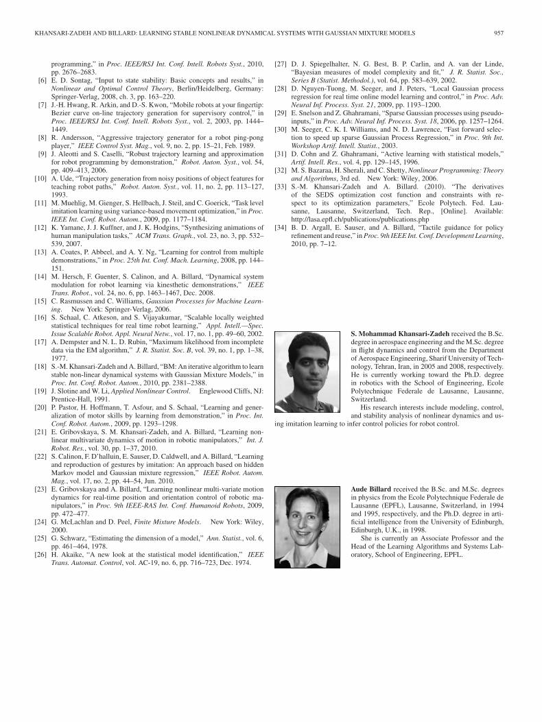
S. Mohammad Khansari-Zadeh received the B.Sc.degree in aerospace engineering and the M.Sc. degreein flight dynamics and control from the Departmentof Aerospace Engineering, Sharif University of Tech-nology, Tehran, Iran, in 2005 and 2008, respectively.He is currently working toward the Ph.D. degreein robotics with the School of Engineering, EcolePolytechnique Federale de Lausanne, Lausanne,Switzerland.

His research interests include modeling, control,and stability analysis of nonlinear dynamics and us-

ing imitation learning to infer control policies for robot control.

Aude Billard received the B.Sc. and M.Sc. degreesin physics from the Ecole Polytechnique Federale deLausanne (EPFL), Lausanne, Switzerland, in 1994and 1995, respectively, and the Ph.D. degree in arti-ficial intelligence from the University of Edinburgh,Edinburgh, U.K., in 1998.

She is currently an Associate Professor and theHead of the Learning Algorithms and Systems Lab-oratory, School of Engineering, EPFL.

learning stable nonlinear dynamical systems with gaussian ... · learning stable nonlinear...

Documents