learning the form of causal relationships using

Learning the Form of Causal Relationships UsingHierarchical Bayesian Models

Christopher G. Lucas and Thomas L. Griffiths

Department of Psychology, University of California, Berkeley

Received 20 January 2009; received in revised form 19 May 2009; accepted 3 June 2009

Abstract

People learn quickly when reasoning about causal relationships, making inferences from limited

data and avoiding spurious inferences. Efficient learning depends on abstract knowledge, which is

often domain or context specific, and much of it must be learned. While such knowledge effects are

well documented, little is known about exactly how we acquire knowledge that constrains learning.

This work focuses on knowledge of the functional form of causal relationships; there are many kinds

of relationships that can apply between causes and their effects, and knowledge of the form such a

relationship takes is important in order to quickly identify the real causes of an observed effect. We

developed a hierarchical Bayesian model of the acquisition of knowledge of the functional form of

causal relationships and tested it in five experimental studies, considering disjunctive and conjunctive

relationships, failure rates, and cross-domain effects. The Bayesian model accurately predicted

human judgments and outperformed several alternative models.

Keywords: Causal reasoning; Bayesian networks; Bayesian models; Hierarchical models; Rational

inference; Structure learning; Human experimentation; Computer simulation

1. Introduction

Causal inference—learning what causal relationships are present in the world by

observing events—is often taken to rely primarily on universal cues such as spatiotempo-

ral contingency or reliable covariation between effects and their prospective causes

(Hume, 1748). While recognizing covariation may be central to causal learning, there is

both experimental and intuitive support for the idea that people also use domain-specific

knowledge. For instance, children come to conclusions that they would not be able to

Correspondence should be sent to Christopher G. Lucas, Department of Psychology, University of California,

Berkeley, 3210 Tolman Hall # 1650, Berkeley, CA 94720-1650. E-mail: [email protected]

Cognitive Science 34 (2010) 113–147Copyright � 2009 Cognitive Science Society, Inc. All rights reserved.ISSN: 0364-0213 print / 1551-6709 onlineDOI: 10.1111/j.1551-6709.2009.01058.x

reach if they were ignorant about the mechanisms behind causal relationships, as shown

by experiments where they pick mechanistically plausible causes over spatially and tem-

porally contingent ones (Shultz, 1982) or prefer mechanical causes for mechanical effects

except when physical constraints make such a relationship unrealistic (Bullock, Gelman,

& Baillargeon, 1982). There is also evidence that this kind of knowledge is learned. For

example, children use mechanism knowledge differently as they age, with older children

showing an understanding of a broader range of mechanisms (Bullock et al., 1982; Shultz,

1982).

Despite these indications that prior knowledge plays a role in causal learning, popular

accounts of causal learning frame prior knowledge as orthogonal to (e.g., Cheng, 1997) or

incompatible with (e.g., Ahn, Kalish, Medin, & Gelman, 1995; Shultz, 1982) statistical

information provided by covariation between causes and effects. Even accounts that accept

that knowledge about mechanisms, domains, and categories need to be combined with

covariation information tend not to provide for how we acquire such knowledge (e.g.,

Waldmann, 1996). The topic has not been ignored, however: In recent years some studies

have explicitly considered the interplay of abstract knowledge and statistical information,

examining how knowledge about categories and the nature of causal relationships affect the

conclusions people draw from covariational evidence (Kemp, Goodman, & Tenenbaum,

2007; Lien & Cheng, 2000; Waldmann, 2007).

In this paper, we present a framework that reconciles covariation-based inference with

acquired knowledge about kinds of causal relationships. Our goal was to explain how chil-

dren and adults extract abstract information about causal relationships from experience and

use this information to guide causal learning. We focus here on knowledge about the

functional form of causal relationships—the nature of the relationship between causes and

effects—and specifically on how causes interact in producing their effects. For example,

imagine a light and two switches. Each switch is connected to the light, and affects whether

the light is on or off. However, there are a variety of ways in which the light and the

switches could be connected: The light might only turn on when both switches are pressed,

or turn on when either is pressed, or turn on only some of the time when either switch is

pressed but more often when both are pressed. Similar possibilities hold for other causal sys-

tems, with causes either acting independently or in conjunction to bring about or prevent

effects. If learners know how causes influence effects in a particular kind of causal system,

they can use this information to inform their reasoning about the existence of causal

relationships.

Our perspective on how people acquire and use knowledge about the functional form of

causal relationships follows in the spirit of rational analysis (Anderson, 1990) and previous

accounts of causal inference (Cheng, 1997): We are concerned with clearly specifying the

underlying computational problem and comparing human inferences to the optimal solution

to this problem. We take the basic challenge of causal induction to be acquiring rich, useful

representations of cause and effect that can be represented using causal graphical models(Pearl, 2000; Spirtes, Glymour, & Schienes, 1993), a formal language for representing

causal relationships, which we describe in more detail below. This formal language allows

us to clearly characterize the role that functional form plays in causal learning, and to

114 C. G. Lucas, T. L. Griffiths ⁄ Cognitive Science 34 (2010)

develop a mathematical framework in which we can analyze how knowledge of functional

form is acquired and used.

We make two contributions toward understanding how people combine prior knowledge

and covariational evidence in causal induction. Our first contribution is showing that the

problem of learning the functional form of a causal relationship can be formalized using

hierarchical Bayesian models, in which information about causal relationships is maintained

at multiple levels of abstraction, reflecting both hypotheses about which causal relationships

exist among specific sets of variables and more general theories about how causes relate to

their effects. This general approach is compatible with other recent work on the acquisition

of causal knowledge (Griffiths & Tenenbaum, 2007; Tenenbaum & Niyogi, 2003) and can

be applied to phenomena beyond those we consider explicitly. Our second contribution is a

series of experiments that test the qualitative predictions made by this approach, as well as

the quantitative predictions made by a specific hierarchical Bayesian model. Our experi-

ments focus on learning about a specific kind of causal system, related to the ‘‘blicket detec-

tor’’ used in previous work on causal learning (Gopnik & Sobel, 2000; Sobel et al., 2004).

We use this system to explore acquisition and use of abstract knowledge about functional

form when the causal structure is specified, as well as when it is learned from contingency

data. We also show that the scope of this knowledge seems to be restricted to the domain in

which it is learned.

The plan of the paper is as follows. The next section reviews previous experiments that

have explored the learning and use of knowledge of functional form. We then summarize

standard accounts of how people infer causal relationships from statistical evidence and con-

sider the role they provide for abstract knowledge. We go on to outline the hierarchical

Bayesian approach to analyzing the role of knowledge in causal induction and indicate how

this approach applies to functional form. This is followed by a series of experiments that test

the predictions of our model, revealing some sources of information that people use and

kinds of knowledge they acquire. We conclude by discussing related models and consider-

ing new questions we hope to answer with this line of work.

2. Using knowledge of functional form in causal induction

Most previous work on the effects of prior knowledge on causal induction has focused on

factors such as the plausibility of a causal relationship (Alloy & Tabachnik, 1984; Koslowski,

1996) and the types of entities in a domain (Lien & Cheng, 2000). However, three studies

have explicitly looked at how people learn and use information about the form of causal

relationships.

Zelazo and Shultz (1989) tested the ability of adults to predict the magnitude of an effect

as a function of two causal variables and found that their inferences depended on the form

of the relationship indicated by the physical system. Specifically, when asked to learn from

two training events and predict how far a counter-weighted balance would tilt or an

obstructed set of blocks would slide, people tended to make inferences consistent with the

dynamics of the specific physical system involved. By contrast, Zelazo and Shultz found

C. G. Lucas, T. L. Griffiths ⁄ Cognitive Science 34 (2010) 115

that 9 year olds’ inferences reflected an understanding that the magnitude of the effect

increased with the size of one block and decreased with the size of the other but did not cap-

ture the differences between specific forms of the two relationships. One interpretation of

this developmental difference is that adults had more experience with the two causal

systems and were thus able to make more precise inferences from the training events.

Waldmann (2007) also found that knowledge of the form of causal relationships strongly

influences evidence-based inference, using a subtler manipulation: He presented adults with

the task of determining the effect of consuming colored liquids on the heart rate of an ani-

mal, varying whether the stated mechanism by which the liquids influenced heart rate was

their taste or their strength as a drug. In the taste case, judgments made by the participants

indicated a tendency to believe that the effect of combining both liquids would be the aver-

age of their individual effects, whereas judgments in the strength case were consistent with

believing the combined effect would be the sum of the individual effects.

Finally, Beckers, De Houwer, Pineno, and Miller (2005) found evidence that the infer-

ences people draw from a set of evidence are shaped by having seen earlier ‘‘pre-training’’

events, suggesting that the magnitude of an effect will be an additive or subadditive function

of its combined causes. Importantly, the different pre-training events did not suggest differ-

ent stories: Beckers et al. only manipulated the strength of the effect in the presence of two

causes, so that in the additive condition it was the sum of the strength of the individual

causes and in the subadditive condition it was the maximum. Participants then saw data

from a standard ‘‘blocking’’ design, in which the effect occurred in the presence of one

cause, A, alone, as well as in the presence of the two causes A and B. Those participants

who had received additive pre-training showed a much stronger blocking effect, believing

that B alone was unlikely to cause the effect as it did not seem to increase the magnitude of

the effect when paired with A. This result is consistent with the assumptions of standard

associative learning models (e.g., Rescorla & Wagner, 1972), which assume additive combi-

nation of causes.

These three studies illustrate that when people make inferences about the presence or

strength of a causal relationship, they are sensitive to the form that any such relationship is

likely to take, and that they can learn the form of a relationship from data. Inspired by these

examples, the remainder of the paper explores the question of how we might use a computa-

tional model to explain how people learn about the functional form of causal relationships

and apply that knowledge. We do this by laying out a general formal framework for model-

ing such learning and then testing the predictions of this approach within a specific causal

system. We start by summarizing the key ideas behind existing models of causal learning.

3. Models of causal learning

Causal learning has been a topic of extensive study in cognitive psychology, resulting in

a large number of formal models of human behavior (for a review, see Perales & Shanks,

2007). Our emphasis here will be on rational models of causal learning: models that explain

human behavior as an optimal solution to a problem posed by the environment (Anderson,


1990; Marr, 1982). In the case of causal learning, the problem amounts to estimating the

strength of a causal relationship or inferring that such a relationship exists (Cheng, 1997;

Griffiths & Tenenbaum, 2005). In this section, we will briefly describe some of the most

prominent rational models of causal learning, dividing these models into those that focus on

learning causal strength and those that focus on learning causal structure. In each case

we will summarize the assumptions that these approaches make about functional

form—strength-based approaches tend to assume a single fixed functional form, while

structure-based approaches make weaker assumptions. First, however, we will describe

the formal language of causal graphical models, which we will use to characterize the

computational problem of causal induction.

3.1. Causal graphical models

Causal graphical models, or causal Bayes nets, are a formalism for representing and rea-

soning about causal relationships (Pearl, 2000; Spirtes et al., 1993). In a causal graphical

model, all relevant variables are represented with nodes, and all direct causal relationships

are represented using directed links, or edges, between nodes. In addition to carrying infor-

mation about statistical relationships between variables, the link structure provides informa-

tion about the effects of interventions and other exogenous influences on a causal system:

Acting to change a variable V may only influence its descendants, that is, variables associ-

ated with nodes reachable by following the links directed away from V.

A causal graphical model depicting the example scenario from the introduction is shown

in Fig. 1, in which one might, by intervening on the states of two switches, influence the

activation of a light. Here, the states of the switches and the activation of the light are the

variables being represented, so each is assigned a node. The links between the switch nodes

and the light node indicate that the switches are direct causes of the light.

Specifying a probability distribution for each variable conditioned on its parents in the

graph (i.e., those variables that are its direct causes) defines a joint distribution on all of the

variables, which can be used to reason about the probability of observing particular events

and the consequences of intervening on the system. However, an edge from one variable to

Fig. 1. Example of a causal graphical model describing the causal relationships behind the operation of a light,

in which two light switches are both causes of its activation.


another in a causal graphical model does not imply a specific functional form for the rela-

tionship between cause and effect. Rather, direct causal (and thus statistical) dependence is

all it indicates.

The full specification of any causal graphical model includes its parameterization, which

defines the probability that any given variable will take a particular value, conditional on its

direct causes. In our example, one might suppose that the probability that the light activates

will be close to zero if either of the switches is not flipped, and close to one otherwise. The

use of probabilities permits reasoning under incomplete information, which applies here as

the reasoner may not know about the internal state of the light—there may be a loose wire

or the filament might be broken. The functional form of a causal relationship is captured by

the parameterization, allowing, for example, the complete causal graphical model to distin-

guish a situation where both switches independently turn on the light from one where a

single switch turns it off, or where the light activates unreliably.

3.2. Learning causal strength

One approach to evaluating a prospective cause c is to take the difference between the

probability of the target effect e in its presence, P(e|c), and the probability of the effect in its

absence, Pðej�cÞ. This quantity, PðejcÞ � Pðej�cÞ, is known as DP, where the probabilities

P(e|c) and Pðej�cÞ are computed directly from contingency data. Proponents of DP argue that

it is a general purpose measure of the strength of a causal relationship (Jenkins & Ward,

1965) as might result from an associative learning process (Shanks, 1995), but it does make

assumptions about the nature of the causal relationship. This can be seen by viewing DPfrom the perspective of learning the structure and parameterization of a causal graphical

model (Griffiths & Tenenbaum, 2005; Tenenbaum & Griffiths, 2001). First, DP assumes that

a particular ‘‘focal set’’ of causes be identified, which is to say that the set of causes or

equivalently the structure of the causal graphical model is known in advance. Second, it

assumes a parameterization under which the probability of the effect given multiple causes

is a linear combination of its probability under separate causes: If the probability of the

effect in the presence of a single cause Ci is wi, then the probability of the effect given the

values of its causes C1,…,Cn is

Pðejc1; . . . ; cnÞ ¼ min 1;XNi¼1

ciwi

!ð1Þ

where ci takes the value one when the ith cause is present, zero otherwise. Under these

assumptions, the value computed by the DP rule for a particular cause Ci is the wi that maxi-

mizes the probability of the events observed by the learner, that is, the maximum likelihood

estimate.

The limitations of DP as a model of human judgments motivated the development of the

Power PC theory (Cheng, 1997), which takes causal learning to be a problem of inferring

the ‘‘causal power’’ of prospective causes. The power of a generative causal relationship is

defined to be


PðejcÞ � Pðej�cÞ1 � Pðej�cÞ ;

which is simply DP divided by the probability of the effect in the absence of the prospective

cause. As with DP, the assumptions of causal power can be made explicit by casting it as

inference about causal graphical models. As before, the structure is assumed a priori via the

choice of focal set, but here the assumption about parameterization is that the probability of

an effect given its causes follows a ‘‘noisy-OR’’ function (Cheng, 1997; Pearl, 1988), in

which each cause has an independent chance to produce its effect (Glymour, 1998; Griffiths

& Tenenbaum, 2005), with

Pðejc1; . . . ; cnÞ ¼ 1�Yni¼1ð1� wiÞci ð2Þ

where ci is defined as in Eq. 1. As with DP, causal power computes the value of wi that

maximizes the probability of the observed events.

Lu, Yuille, Liljeholm, Cheng, and Holyoak (2007, 2008) recently proposed an extension

of the causal power model in which Bayesian inference is used to identify the strength of a

causal relationship. In this model, a prior distribution is defined on the strength of the rela-

tionship wi, either being uniform or favoring stronger relationships, and this information is

combined with contingency data to obtain a posterior distribution. A single estimate of the

strength can be derived from this posterior distribution in several ways, such as taking the

most probable or the average value. The basic assumptions behind this model are the same

as those of the earlier causal power model (Cheng, 1997), taking the noisy-OR to be the

appropriate functional form for the causal relationship, but Lu et al. (2007) and Lu, Rojas,

Beckers, and Yuille (2008) showed that using an appropriate prior can improve the predic-

tions that the model makes.

Finally, Novick and Cheng (2004) explored a way of extending the causal power

model to accommodate relationships between multiple causes that go beyond the noisy-

OR. In this extension, interactions between causes are handled by introducing new vari-

ables that represent combinations of causes. By considering possible generative and

inhibitory effects of both the simple causes and their combinations, this model is capa-

ble of expressing a richer repertoire of functional forms. Yuille and Lu (2007) have

shown that this approach can be used to capture any pattern of dependencies between

multiple causes and an effect, with any conditional distribution being expressible as a

combination of noisy logic gates.

3.3. Learning causal structure

While DP and causal power are rational measures of the strength of a causal relationship

given certain assumptions about the nature of those relationships, another recent work has

explored an alternative view of the problem of causal induction, focusing on the structuraldecision as to whether a causal relationship exists rather than its strength (Griffiths &


Tenenbaum, 2005). There are two general approaches to learning what causal structure

underlies a set of observations.

The first approach to structure learning has been called the ‘‘constraint-based’’ approach

and involves using statistical tests of independence (such as chi-squared) to determine which

variables are related to one another and then reasoning deductively from patterns of depen-

dencies to causal structures (e.g., Pearl, 2000; Spirtes et al., 1993). Constraint-based causal

learning typically makes no assumptions about the nature of causal relationships, using sta-

tistical tests to search for violations of statistical independence and exploiting the fact that

the structure of a graphical model implies certain independence relations, to identify the

causal structure underlying the available evidence. This makes it possible to recover causal

structures regardless of the functional form of the underlying relationships. However, this

flexibility comes at the cost of efficiency. People can learn causal relationships from just a

few observations of cause and effect (Gopnik & Sobel, 2000; Shultz, 1982), but constraint-

based algorithms require relatively large numbers of data to determine causal structure

(enough to produce statistical significance in a test of independence).1

The second approach to structure learning is to frame causal induction as a problem of

Bayesian inference. In this approach, a learner must determine which hypothetical causal

graphical model h is likely to be the true one, given observed data d and a set of beliefs

about the plausibility of different models encoded in the prior probability distribution P(h).Answering this question requires computing the posterior probability P(h|d), which can be

found by applying Bayes’ rule

PðhjdÞ ¼ PðdjhÞPðhÞPh0 Pðdjh0ÞPðh0Þ

ð3Þ

where P(d|h) indicates the probability of observing d assuming that h is true, and is known

as the likelihood. The likelihood is computed using the probability distribution associated

with the causal graphical model h, and thus reflects the expectations of the learner about the

functional form of causal relationships. However, in applications of Bayesian structure

learning in machine learning (e.g., Cooper & Herskovits, 1992), minimal assumptions are

made about the functional form of causal relationships—typically just that the probability of

the effect differs in the presence and absence of a cause.

4. Modeling the effects of knowledge of functional form

The models of causal induction outlined in the previous section provide a basic frame-

work in which to explore how prior knowledge influences the inferences that people make

about causal relationships. However, none of these models directly addresses the problem of

learning the functional form of a causal relationship and using that knowledge to inform

future causal learning. Existing models either assume that causal relationships have a

specific functional form or make no assumptions about the functional form of a causal rela-

tionship. Causal power and DP do not allow for the possibility that people might assume


different functional forms in different contexts, and constraint-based algorithms and

standard Bayesian structure learning invoke minimal knowledge at the cost of efficiency.

However, the Bayesian approach to causal learning provides us with the tools we need in

order to explore how knowledge of functional form affects causal induction and how this

knowledge is acquired. We will focus on learning causal structure, although a similar

approach could be applied for learning causal strength.

4.1. Using knowledge of functional form

Bayesian inference uses two pieces of abstract knowledge. The first is some prior beliefs

about which hypotheses are more likely than others, encoded in the prior distribution P(h).The second is a set of expectations about what effects one should observe given that certain

causes are present, encoded in the likelihood function P(d|h). While most Bayesian structure

learning algorithms make relatively generic assumptions about the prior and likelihood, we

can make stronger assumptions in order to reflect the knowledge that learners possess. In

particular, we can capture knowledge about the functional form of a causal relationship

through our choice of likelihood.

We assume that the causal structures under consideration contain variables in two classes

(prospective causes and effects), that the class to which each variable belongs is known, and

that the only relationships that could potentially exist are those between causes and effects.

The data, d, are events observed by the learner, consisting of causes being present or absent

and effects either occurring or not. We also assume that the events in d are independent once

the underlying causal structure is known, so that P(d|h) ¼ PkP(dk|h) where dk is a single

event. Finally, we assume that the probability of a cause being present in a given event does

not depend on the causal structure h, with the causal structure merely determining the proba-

bility that the effect occurs. Defining the likelihood then reduces to specifying the probabil-

ity with which the effect occurs, given the number of its causes that are present.

Returning to the example of the light, different mechanisms translate into different proba-

bilities for certain events, and consequently different likelihood functions. For instance, one

might expect that a deterministic conjunctive function applies, giving the effect probability

1 when all causes are present, and 0 otherwise.2 Alternately, a deterministic disjunctive

function might apply, giving the effect probability 1 when at least one cause is present, and

0 otherwise. If there is reason to believe a noisy-OR relationship is at work, the probability

of the effect is given by Eq. 2, as discussed previously.

Assuming that a causal system follows a specific functional form such as one of the above

provides constraints that aid causal learning. For example, under a disjunctive function with-

out background causes, just one observation of the presence of a cause and the occurrence

of the effect is sufficient to indicate that a causal relationship exists. By exploiting this kind

of information, Bayesian models incorporating knowledge about the functional form of cau-

sal relationships are capable of identifying causal structure from limited data in the same

way as human learners (Tenenbaum & Griffiths, 2003).

This approach to characterizing how knowledge of functional form might be used is con-

sistent with previous work in causal learning. The idea that the functional form is expressed


through the likelihood, defining the probability of the effect given the cause, is standard in

statistical interpretations of causal strength estimation (Cheng, 1997; Glymour, 1998;

Griffiths & Tenenbaum, 2005; Lu et al., 2007, 2008). These models allow for a variety of

functional forms, including noisy-OR relationships and their generalization to incorporate

interactions and other kinds of noisy-logical circuits (Novick & Cheng, 2004; Yuille & Lu,

2007). By considering functional forms that allow linear combinations of causes (including

averaging), the results of Waldmann (2007) and Beckers et al. (2005) could also be accom-

modated within this framework. However, a more significant challenge is explaining how

people acquire knowledge of functional form that is appropriate to a given domain.

4.2. Learning causal theories

Bayesian inference provides a simple way to make use of abstract knowledge about the

functional form of a causal relationship. More generally, the abstract knowledge needed to

perform Bayesian inference can be expressed as a ‘‘theory’’ about a domain, identifying

types of objects, the plausibility of causal relationships, and the form of those relationships

(Griffiths, 2005; Griffiths & Tenenbaum, 2007). The Bayesian approach also allows us to

analyze how these theories themselves might be learned. The notion that we learn theo-

ries—complex, abstract, and consistent representations that like scientific theories reflect

and facilitate inference about the structure of the real world—has a long history in cognitive

development (Carey, 1991; Gopnik & Wellman, 1992). Recent work in computational mod-

eling of causal learning has begun to extend the Bayesian approach to inferring the structure

of causal graphical models to the level of theories, using hierarchical Bayesian models

(Griffiths & Tenenbaum, 2007; Tenenbaum & Griffiths, 2003).

The basic idea behind a hierarchical Bayesian model is to perform probabilistic inference

at multiple levels of abstraction. In the case of causal learning, these levels are the hypothet-

ical causal graphical models under consideration—the hypotheses h we have been discuss-

ing so far—and the abstract theories that generalize over these hypotheses. In the resulting

probabilistic model, we assume that each theory t defines a probability distribution over

hypotheses P(h|t), just as each hypothesis defines a probability distribution over data,

P(d|h). To return to the example of the light and switches, we might thus characterize our

knowledge of how electrical systems tend to work in terms of a probability distribution over

a set of causal graphical models that differ in their parameterization, reflecting conjunctive,

disjunctive, or other possible kinds of relationships. Each kind of parameterization would

correspond to a different theory, t, with each theory defining a prior distribution over causal

graphical models featuring that parameterization.

Like structure learning, theory learning can be reduced to a problem of Bayesian inference.

If our goal is to infer a theory t from data d, we can do this by applying Bayes’ rule, with

PðtjdÞ ¼ PðdjtÞPðtÞPt0 Pðdjt0ÞPðt0Þ

ð4Þ

where P(t) is a prior distribution on theories. The likelihood P(d|t) is obtained by summing

over all hypothetical causal structures, with P(d|t) ¼P

hP(d|h,t)P(h|t) where P(d|h,t) is the


probability of the data given the structural hypothesis h under the theory t (reflecting the

assumptions of the theory about the functional form of a causal relationship) and P(h|t) is

the probability of that hypothesis given the theory (reflecting assumptions about the plausi-

bility of particular relationships).

Equation 4 applies Bayes’ rule in the same way as it was applied to hypothetical causal

structures in Eq. 3. However, theories are defined at a higher level of abstraction than

hypotheses about the causal structure relating a specific set of variables. As a consequence,

this knowledge supports generalization. For example, upon learning that two switches need

to be pressed in order to turn on a light, a learner might believe that a conjunctive relation-

ship is likely to apply in similar settings in the future. The idea that unknown variables can

be shared across data sets is at the heart of hierarchical Bayesian models (for details, see

Gelman, Carlin, Stern, & Rubin, 1995) and makes it possible for information from one data

set to guide inferences from a second. More formally, learners who encounter a data set d (1)

can update their posterior distributions over theories, computing P(t|d (1)) as in Eq. 4. Upon

encountering more data, d (2) in a similar setting, this posterior distribution over theories can

be used to guide inferences about causal structure. Specifically, it takes the role of the prior

over theories for interpreting the new data. The joint distribution on hypotheses and theories

is given by

Pðh; tjd ð1Þ; d ð2ÞÞ / Pðd ð2Þjh; tÞPðhjtÞPðtjd ð1ÞÞ ð5Þ

where the constant of proportionality is obtained by normalizing the distribution to sum to

one over all h and t. The probability of a given causal structure is then obtained by summing

over all theories, with

Pðhjd ð1Þ; d ð2ÞÞ ¼Xt

Pðh; tjd ð1Þ; d ð2ÞÞ ð6Þ

allowing the abstract knowledge about causal relationships gleaned from d (1) to influence

the conclusions drawn from d (2). Hierarchical Bayesian models thus allow learners to iden-

tify the abstract principles that organize a domain, updating their expectations as more data

are observed.

This account of how knowledge of functional form can be acquired is the main novel

contribution of our approach. It provides a way to understand how learners might make

inferences about functional form from observing a causal system, and then use this knowl-

edge later when learning about causal relationships. It differs from the previous approaches

to modeling causal learning discussed above in allowing learners to flexibly identify a spe-

cific functional form for causal relationships in a given setting, instead of assuming a fixed

functional form for all causal relationships, or making weak and generic assumptions about

functional form. A similar approach was recently used by Lu, Rojas, Beckers, and Yuille

(2008) to explain the results of Beckers et al. (2005) (for details, Section 11) and could be

used to explain how children and adults form generalizations about the relationship between

physical variables in the experiments of Zelazo and Shultz (1989), with different kinds of

relationships corresponding to different causal theories. However, we chose to test the


predictions of this account by considering a novel causal system in which we can manipu-

late a variety of factors related to functional form.

5. Testing the predictions of the hierarchical Bayesian approach

The approach outlined in the previous section can be applied to the problem of acquiring

and using knowledge of the functional form of causal relationships: Abstract theories can

express different assumptions about functional form, allowing learners to infer what kind of

functional form is most appropriate for a given domain. There are two qualitative predic-

tions that distinguish this hierarchical Bayesian approach from other models of causal learn-

ing: (a) that people can make inferences appropriate to causal relationships with more than

one kind of functional form and (b) that people can use evidence from one data set to inform

their inferences from another involving different variables. In the remainder of the paper we

present a test of these predictions, using a specific causal system to explore whether people

can form generalizations about the functional form underlying a causal relationship and

what factors influence this process. To do so, we use a causal inference problem in which

knowledge of functional form is important, not known in advance, and which permits us to

generate quantitative predictions with a specific hierarchical Bayesian model.

Suppose a learner is faced with the problem of identifying which of a set of objects are

‘‘blickets’’ using a ‘‘blicketosity meter’’ knowing only that blickets possess something

called blicketosity and that the meter sometimes lights up and plays music (activates).3 The

hypotheses under consideration by the learner are partitions of objects into blicket and non-

blicket classes. As activating the meter is the result of a causal relationship between the

object and the detector, these hypotheses can be expressed as causal graphical models,

where objects are prospective causes, activation is the effect, and a causal relationship exists

between cause and effect if and only if the corresponding object is a blicket.

Crucially, two objects can be placed on the blicketosity meter simultaneously, making it

possible to explore different functional forms for the underlying causal relationship. Differ-

ent functional forms have strong implications for how the learner should interpret different

events. For instance, if the learner believes that two blickets’ worth of blicketosity are nec-

essary to activate the meter, then seeing a single object failing to activate the meter is unin-

formative. Under such a belief, two objects that together activate the meter are both

blickets, whereas that event under a disjunctive relationship suggests only that one or both

of the objects is probably a blicket.

If people assume that the functional form of a causal relationship is fixed (e.g., linear or

noisy-OR), or they make minimal assumptions about the functional form of causal relation-

ships, then they will make the same inferences about casual structure regardless of evidence

about functional form. Consequently, testing predictions in cases where structural inferences

are guided by knowledge of functional form is a way to evaluate the central claims of a hier-

archical Bayesian approach: that people entertain abstract theories about the functional form

of causal relationships and update their beliefs about these theories in light of evidence.

This logic motivated the experiments that we present in this paper. In describing these


experiments, we will also define a specific hierarchical Bayesian model, constructed by

choosing likelihoods and priors that are simple, flexible, and appropriate to the cover story

given to participants, and compare its numerical predictions to those generated by other

models of causal inference.

In our experiments, participants were first presented with one of three sets of events

involving three objects (A, B, C).4 Participants saw events that had high probability under

either a deterministic disjunctive, conjunctive, or noisy disjunctive theory (see Table 1).

Next, all groups saw a set of events with three new objects (D, E, F) that was compatible

with any of the three theories, D)D)D) E) DF+ DF+, that is, object D failing to activate

the meter three times, E failing once, and a combination of D and F succeeding twice. If

participants acquired knowledge about functional form using the first block of evidence,

then they would be expected to come to different conclusions about which objects in the

second were blickets.

Using the terms introduced in the previous section, the events involving A, B, and C form

an initial data set d (1), and the events involving D, E, and F form a second data set d (2).

After seeing d (1), learners can compute a posterior distribution over theories, P(t|d (1)) by

applying Eq. 4. This posterior distribution informs inferences about the hypothetical causal

structures that could explain d (2), as outlined in Eqs. 5 and 6. The key prediction is that

varying d (1) should affect inferences from d (2). This prediction is not made by any non-

hierarchical model, because the events in d (1) do not involve any of the prospective causes

in d (2). Without abstract acquired knowledge that spans multiple contexts, there is no conti-

nuity between the two sets of evidence.

While the qualitative predictions tested in our experiments are made by any hierarchical

Bayesian model, we can also obtain quantitative predictions by considering a specific model

that gives values to P(d|h,t), P(h|t), and P(t). The appropriate model will depend on the con-

text, as the hypotheses and theories that are relevant may vary. Our goal was thus not to

define a general purpose model that could explain all instances of learning of functional

form, but a simple model appropriate for characterizing the inferences that people make

about functional form for the blicketosity meter. The main purpose of developing this model

was to illustrate how people’s judgments should be affected by our experimental manipula-

tions, assuming a reasonable but relatively restricted set of possible functional forms.

Our hierarchical Bayesian model is defined in terms of the distributions P(d|h,t), P(h|t),and P(t). We will discuss P(h|t) first, then turn to P(d|h,t) and P(t). This is partly motivated

by the fact that P(h|t) is the simplest part of the model: We take all hypotheses regarding

causal structure to be a priori equally likely, yielding P(h|t) ¼ P(h) where P(h) is identical

Table 1

Evidence presented to participants in Experiment 1

Block Evidence Blicket

Conjunctive training A)B)C)AB)AC+BC) A, CNoisy-disjunctive training A+B)C)AB)AC+BC) ADeterministic disjunctive training A+B)C)AB+AC+BC) ATest D)D)D)E)DF+DF+


for all structures. If the learner learns what the causal structure is (e.g., he or she is told what

causal structure is present in the training block), then P(h) is updated to reflect that knowl-

edge, so that the probability of the known structure becomes 1.

As for P(d|h,t), we have already provided examples of how different functional forms

might translate into likelihood functions, and we chose for our model a space of theories that

can approximate noisy-OR, AND, and other relationships while being broadly compatible

with the cover story provided to participants and requiring a small number of parameters.

Specifically, we selected a sigmoid likelihood function:

PðejNblickets ¼ nÞ ¼ 1

1þ expf�gðn� bÞg ð7Þ

where Nblickets is the number of blickets among the present objects, b is the bias (i.e., the

number of blickets necessary to make the meter equally likely to activate as not), and g gives

the gain of the function. To give a sense of the generality of this function, when b ¼ 0.5 and

g >> 1 one obtains a deterministic-OR function, b ¼ 1.5, g >> 1 gives a deterministic con-

junctive function, and b ¼ 0.81, g ¼ 7.37 closely approximates a noisy-OR function with

wi ¼ 0.8 for all i (see Fig. 2). Under this specification, the theory held by a learner amounts

to his or her beliefs about the probable values of b and g.

Finally, we must provide a prior over theories, which under our model amounts to a prob-

ability density for b and g. For the sake of simplicity, we chose exponential priors for both band g, each with a single hyperparameter (kb and kg) setting how rapidly the probabilities

of values of b and g decrease. The probabilities of b and g were thus proportional to

exp {)kbb} and exp {)kgg}, respectively. If the mean of the prior distribution for the bias

parameter is less than one (i.e., kb > 1), the prior beliefs favor disjunctive relationships,

while a large value for the hyperparameter for the gain, kg, favors deterministic rather than

noisy functions.5 While we believe that our specification for the space of functional forms is

generally appropriate for the cover stories in our experiments, we do not assert that it

encompasses all theories that people can entertain. For example, Shanks and Darby (1998)

discuss an experiment in which people learn that causes can independently bring about an

effect but jointly do not, a functional form that cannot be specified in terms of the logistic

function. We return to the issue of more general models of functional form learning in the

Section 11.

With the training data we selected, our model predicts a disordinal interaction in which

the rank order of the ratings for objects D and E reverses: In the conjunctive conditions

object D was expected to be judged more likely to be a blicket than object E, and vice versa

in the disjunctive conditions. This interaction, which emerges with a wide range of plausible

values for kb and kg, is a consequence of the fact that the D) events should be taken as evi-

dence against D being a blicket under a disjunctive theory, while under a conjunctive theory

the D) events are uninformative and the DF+ events indicate that D is a blicket. To make

the quantitative predictions that we test in our experiments, a single value for each of kb and

kg was chosen to minimize sum-squared error when compared with participants’ ratings

over all experiments, resulting in kb¼4.329 and kg¼0.299. The predictions were fairly

insensitive to these values, a point that we explore in detail in Section 11.


In the remainder of the paper we present a series of experiments testing the predictions

that discriminate our account from others. Experiment 1 examines learning about the func-

tional form of causal relationships when the causal structure is known. Experiment 2

addresses the problem of learning about causal structure and functional form simulta-

neously, and Experiment 3 provides control conditions to confirm our interpretations of the

results of Experiment 2. Experiment 4 tests additional predictions about the consequences

of acquiring knowledge about functional forms, and Experiment 5 deals with the domain

specificity of this knowledge.

6. Experiment 1: Known causal structure

Experiment 1 was designed to be a direct test of the predictions that distinguish a hierar-

chical Bayesian account from others, namely that events involving one set of variables will

influence later inferences drawn about a different set of variables. Here, we simplified the

Fig. 2. Examples of different kinds of relationship forms expressed as sigmoid functions.


task by providing participants with the causal structure behind the first event set, leaving

them only the problem of learning about functional form.

6.1. Methods

6.1.1. ParticipantsParticipants were 57 undergraduates from the University of California, Berkeley,

who received course credit for participation. These participants were divided into deter-ministic disjunctive (n ¼ 20), noisy-disjunctive (n ¼ 20), and conjunctive (n ¼ 17)

conditions.

6.1.2. Materials and procedureThe stimuli were six identical beige 2¢¢ · 2¢¢ · 2¢¢ cubes, labeled A, B, C, D, E, and F, and

a green 5¢¢ · 7¢¢ · 3¢¢ box with a translucent orange panel on top, called a ‘‘blicketosity

meter.’’ A hidden foot-controlled switch allowed the experimenter to toggle the meter

between a state in which it activated when objects were placed on it and a state in which it

did not. When activated, the box played a short melody and the orange panel was illumi-

nated by a light inside.

The experiment consisted of two trials. In the first trial, participants were told that some

blocks are blickets, some are not, and that blickets possess blicketosity, while nonblickets

possess no blicketosity. They were also told that the blicketosity meter had a binary

response: It could either activate or not. One or two objects were then identified as blickets

(see Table 1, third column). They were given no more information about the nature of

blickets or the blicketosity meter. The experimenter provided participants with evidence by

placing the first three objects (A, B, and C), singly or in groups, on the box. By surrepti-

tiously toggling the hidden foot switch, the experimenter was able to control which combi-

nations of objects appeared to activate the machine. There were three different training

evidence conditions, labeled by the form of causal relationship they suggested: determinis-tic-disjunctive, noisy-disjunctive, and conjunctive. Table 1 gives the specific events

presented in each condition.

After the training block was presented, the objects were set aside, and three new objects

labeled D, E, and F were introduced. Participants then saw a block of test evidence that was

the same across all conditions, D) D) D) E) DF+ DF+. These specific events were chosen

to lead to different beliefs about which objects were blickets, depending on what kind of

relationship participants believed applied.

After participants saw the evidence in the test block, they recorded the probability they

assigned to each of the test objects D, E, and F being blickets on a 0–10 scale, having been

told that a 10 indicated they were absolutely certain the object was a blicket, a 0 indicated

absolute certainty it was not, and a 5 indicated that it was equally likely to be a blicket as

not.

Finally, after all participants had recorded their ratings, they were prompted to record in

plain English their theories of how the meter interacted with blickets and nonblickets, and

how the meter operated.


6.2. Results and discussion

The mean ratings are shown in Fig. 3. The prediction that causal knowledge derived from

one set of objects constrains subsequent inferences was supported: One-way anovas found

an effect of the Trial 1 data on judgments in Trial 2 for both object D (F[2,54] ¼58.1, p < 0.001, g2 ¼ 0.68) and object E (F[2,54] ¼ 11.353, p < 0.001, g2 ¼ 0.2). The

specific effects we expected were that object D would be given higher ratings in the con-junctive condition than in the deterministic-disjunctive condition, and that object E would

have a higher rating in the noisy-disjunctive condition than in the deterministic-disjunctivecondition. We found support for the first of these effects (t[35] ¼ 8.759, p < 0.001, d ¼1.64) and a trend consistent with the second (t[38] ¼ )1.603, p ¼ 0.117, d ¼ )0.50). The

data also supported the hypothesis that many participants in the conjunctive test block were

inferring that a conjunctive relationship applied to the events: the mean rating of D in the

conjunctive condition was significantly higher than 5(t[16] ¼ 3.15, p < 0.01, d ¼ 0.76),

indicating that D was considered more likely than not to be a blicket, something that is

inconsistent with all linear and noisy-disjunctive interpretations.6

The numerical predictions of our model closely matched participants’ behavior: The

within-condition rank orders of ratings were in perfect agreement, mean-squared error was

0.38, and the linear correlation between the ratings and participants’ judgments was 0.99.

We can evaluate the performance of the model by comparing it with alternative models that

also make quantitative predictions. As mentioned previously, DP and causal power do not

predict that responses will vary between any of our conditions. Under DP, the predicted

response for D is PðejDÞ � Pðej �DÞ, or 25, for a rating of 4. Causal power normalizes that

quantity by 1 � Pðej �DÞ, also giving 4 for D. The predicted ratings for E and F under both

DP and causal power are 0 and 10, respectively. These models’ predictions are accurate in

the disjunctive conditions where their assumptions regarding functional form are appropri-

ate, but in the conjunctive condition their predictions diverge from the data, leading to an

Fig. 3. Results of Experiment 1, showing the model predictions and human ratings of the probability that test

condition objects are blickets.


overall mean-squared error per rating of 5.83 and a correlation of 0.82 with human ratings.

We will evaluate some extensions of these models in Section 11.

We can also compare the performance of our model with that of the best possible model

that is blind to the training evidence. This model would make optimal predictions for the rat-

ings of D, E, and F, under the constraint that the ratings must be the same across all three

conditions. The best predictions for D, E, and F—in terms of minimizing error and maxi-

mizing correlation—are equal to their observed means across all three conditions. Such pre-

dictions yield a mean-squared error of 3.97 and a linear correlation of 0.83. The best

possible model that ignores condition thus performs much worse than our Bayesian model,

as this model fails to capture the change in ratings produced by providing different informa-

tion about the functional form of the causal relationship.

In order to establish that participants’ ratings reflected their beliefs about the form of the

causal relationships and were likely to generalize appropriately to evidence beyond that pro-

vided in our experiment, we analyzed the plain English theories participants expressed after

the second trial. Two hypothesis- and condition-blind research assistants coded participants’

theories about how the meter worked, resolving any differences through discussion. The fea-

tures recorded for each theory included the following: (a) whether the theory was interpret-

able, (b) whether blickets and nonblickets increased, decreased, or had no influence on the

probability of the effect, (c) whether the effect was perfectly, imperfectly, or not predictable

given its observable causes, and (d) whether the relationship was conjunctive. The overall

proportion of theories that was interpretable was 0.74, and it did not differ significantly

between conditions (Fisher’s exact text, p > 0.5).

Differences in participants’ explicit theories were consistent with learning about the form

of the causal relationship: A greater proportion of interpretable theories in the conjunctivecondition were consistent with a conjunctive relationship (12 of 13) than in the determinis-tic- and noisy-disjunctive conditions (3 of 16 and 4 of 13, respectively) (Fisher’s exact test,

p < 0.01). Participants in the noisy-disjunctive condition expressed theories that involved

noise or imperfect predictive ability more frequently (5 of 13 interpretable theories versus 1

of 16 for the deterministic-disjunctive condition and 0 of 13 for the conjunctive condition;

Fisher’s exact test, p < 0.05).

The results of the experiment support our account of causal learning: People developed

different theories about the functional form of the causal relationship, and they used these

theories when reasoning about the existence of individual causal relationships. However, as

people were provided with information about the relationships that existed among the objects

presented in the training block, this remains a modest test of their ability to learn the functional

form of causal relationships. As a more ambitious test, we conducted Experiment 2, in which

participants were forced to learn about causal structure and functional form simultaneously.

7. Experiment 2: Unknown causal structure

Having found the predicted pattern of judgments when participants knew which train-

ing objects were blickets, we conducted Experiment 2 to test the prediction that people


can concurrently learn about the causal structure and functional form of causal relation-

ships. We did this using a procedure identical to Experiment 1, save that we withheld

the identities of the blickets in the training block, effectively hiding the underlying

causal structure. In addition, we took the opportunity to address an alternative interpre-

tation of the results of Experiment 1, under which participants took there to be the

same number of blickets in both blocks of evidence and mapped objects in the test

block to objects in the training block. We ran a new condition to test this possibility,

in which participants saw evidence that was probably given a deterministic-OR relation-

ship and two blickets. If the alternative explanation were true, then participants would

be expected to pick out two of the D, E, and F objects as blickets. If people are using

information about the functional form of causal relationships to make inferences in the

test condition, then their judgments should be similar to those in the one-blicket

deterministic disjunctive condition.

7.1. Methods

7.1.1. ParticipantsParticipants were 102 undergraduates from the University of California, Berkeley, who

received course credit for participation, again divided into deterministic-disjunctive (n ¼26), noisy-disjunctive (n ¼ 26), and conjunctive (n ¼ 24) conditions, with an additional

deterministic disjunctive base-rate control (n ¼ 26) condition.

7.1.2. Materials and procedureThe first three conditions were identical to those in Experiment 1, but participants were

told nothing about which objects were blickets in the training block, and instead were asked

to provide probabilities as in the test block. These will again be referred to as the determinis-tic-disjunctive, noisy-disjunctive, and conjunctive conditions. The base-rate control condi-

tion was an additional control to establish that participants were not merely using base-rate

information to infer that a specific number of blickets were present in the test block. The

evidence participants saw was intended to be compatible with a deterministic disjunctive

relationship, but with two blickets present rather than one. The procedure was the same as

in the previous three conditions, but the specific training evidence participants saw was

A+ B+ C) AB+ AC+ BC+.


Our first analyses focused on the three conditions from Experiment 1, the deterministic-disjunctive, noisy-disjunctive, and conjunctive conditions. As in Experiment 1, there was an

effect of the training block on judgments in Trial 2 for D (F[2,73] ¼ 6.026, p < 0.01, g2 ¼0.14). More specifically, object D was given higher ratings in the conjunctive condition than

in the deterministic-disjunctive condition (t[48] ¼ 3.472, p < 0.01, d ¼ 0.89). Contrary to

our predictions, the mean rating given to object E was not higher in the noisy-disjunctivecondition than in the conjunctive condition, which we discuss below. With the exception of


this reversal, the ordinal match between numerical predictions of our model and partici-

pants’ ratings was exact. Mean-squared error was 0.29 and the linear correlation between

the predictions and participants’ ratings was 0.99. The mean ratings and model predictions

are shown in Fig. 4. For comparison, the predictions of both DP and causal power yielded

an MSE of 4.03 and a correlation of 0.90. Because the ratings varied less between condi-

tions, the best-possible training-blind predictions were better than in Experiment 1, giving

an MSE of 0.63 and a correlation of 0.97. As in Experiment 1, participants’ explicit theories

mentioned conjunctive relationships more often in the conjunctive condition (13 of 17) than

in the noisy-disjunctive (6 of 23) and deterministic-disjunctive (5 of 23) conditions (Fisher’s

exact test, p < 0.001)

In retrospect, the higher-than-expected rating for D in the noisy-disjunctive condition is

unsurprising given that the training events were also compatible with complex deterministic

theories, and previous work suggests that people tend to believe that complex deterministic

causal relationships are more likely than simple stochastic relationships (Schulz & Sommer-

ville, 2006). The theories participants expressed were compatible with this interpretation:

only 13% (3 of 23) of the interpretable theories mentioned noise or an imperfectly predict-

able effect versus 38% (5 of 13) in the noisy-disjunctive condition of Experiment 1, although

this difference was not significant (Fisher’s exact test, p ¼ 0.11). If people are inferring that

deterministic relationships outside our space of theories apply, then making it clear that the




generative relationship is subject to occasional failure will bring participants’ ratings back

in line with our predictions. We explore this possibility in the next experiment.

Finally, the results of our additional control condition were consistent with our account.

In the base-rate control condition the mean ratings for objects D and E were lower than in

the original deterministic-disjunctive condition, giving a larger effect when comparing

conjunctive condition ratings for D (t[48] ¼ 4.18, p < 0.001, d ¼ 1.02), as predicted by our

model and contrary to what an alternative explanation based on the frequency with which

blickets appear in the training data would predict.

8. Experiment 3: The effects of noise

In Experiment 2 we found that participants’ judgments in the noisy-disjunctive condition

deviated from the predictions of our model, and we speculated that participants were infer-

ring that complex deterministic relationships produced the events. To test whether this was

the case, we ran two new conditions in which we provided explicit evidence that the meter

was subject to unpredictable failures to activate. In the first, we gave participants training

events that were incompatible with a deterministic explanation by prepending two failure

events (A) A)) to the noisy-disjunctive data in Experiment 2. In the second we told partici-

pants that the meter was failure prone. If participants’ unexpected judgments in Experiment

2 were the result of their rejecting the possibility that the relationship was noisy, then both

interventions should lead to ratings for D being lower than those for E.

8.1. Methods


received course credit for participation, divided into event-based noise (n ¼ 3) and

description-based noise (n ¼ 28) conditions.

8.1.2. Materials and procedureThe two conditions used a procedure based on that in the noisy-disjunctive condition of

Experiment 2. In the description-based noise condition participants were told, ‘‘Sometimes,

the blicketosity meter randomly fails to go off when it should.’’ The event-based noise con-

dition added two events in which object A failed to activate the meter to the noisy-disjunc-tive training block, so that participants saw the events A+ A) A) B) C) AB) AC+ BC) in

the training block. The two conditions were otherwise identical. As in Experiments 1 and 2,

the test evidence was D) D) D) E) DF+ DF+.


Under both manipulations, the mean participant ratings for D were lower than E, a result-

that was significant after aggregating data from the two manipulations (t[40] ¼ )2.03,


p ¼ 0.049, d ¼ 0.32). Comparing the effect of these two manipulations on the difference

between the D and E ratings with the D ) E difference in the noisy-disjunctive condition of

Experiment 2, yielded a significant difference in the description-based noise condition

(t[52] ¼ 2.41, p ¼ 0.019, d ¼ 0.63), and a trend in the event-based noise condition

(t[37] ¼ 1.92, p ¼ 0.062, d ¼ 0.63).

The correlation between the ratings of participants and the predictions of the model was

0.98, and the mean-squared error was 0.55. Mean ratings and model predictions are given in

Fig. 5. With this indication that people make the inferences one would expect when they

have evidence for a failure-prone system, we can test another prediction of our model: that

people can use covariation evidence to learn how noisy a class of causal relationships is and

use that information to make more accurate inferences about causal structures involving

novel objects.

9. Experiment 4: Manipulating causal strength

If people are transferring knowledge about the strength of the relationship between

the presence of blickets and activation of the meter, then one would expect to see dif-

ferent ratings for the probability of D, E, and F being blickets as the training set is

manipulated to suggest higher or lower failure rates for the meter. Specifically, our

intuitions and model predict that the probability that D is a blicket given the test data

are higher under a high failure rate noisy-disjunctive relationship than one that fails

infrequently; under a nearly failure-free relationship, the three failures to activate under

D constitute strong evidence against D being a blicket, while the evidence against E—a

single failure—is weaker. At the opposite extreme, when the meter rarely activates for

a blicket, the three failures constitute weak evidence that D is not a blicket, while the

activation under D and F together is now positive evidence for D being a blicket. We

tested this prediction with another experiment.




9.1. Methods


received course credit for participation, divided into high-noise (n ¼ 20) and low-noise(n ¼ 21) conditions. One participant was excluded for explaining that the blicketosity meter

detected nonblickets.

9.1.2. Materials and procedureThe procedure was similar to that used in the event-based noise condition in Experiment

3, but the evidence was varied between two conditions to indicate different failure rates.

The evidence in the low-noise condition was A+ A+ A+ A) A+ A+ B) C) AB) AC+ BC),

where the meter activated five out of six times given object A alone. The evidence in the

high-noise condition was A) A) A) A+ A) A) B) C) AB) AC+ BC), where the meter

activated one out of six times given object A alone.


The mean rating for D was higher in the high-noise condition (3.8, SD 2.4) than in the

low-noise condition (1.8, SD 2.4), (t[39] ¼ 2.57, p ¼ 0.014, d ¼ 0.753), consistent with

the predictions of the model. As in the previous experiments, the quantitative predictions of

the model were accurate, with a correlation with ratings of 0.98 and a mean-squared error of

0.52.

At this point we have shown that people used covariational evidence to learn about

the functional form of causal relationships—including whether the basic structure of

the relationship was conjunctive or disjunctive, and the strength of disjunctive relation-

ships—and used that knowledge to guide their later inferences. However, it might be

argued that what we have observed was not the acquisition of abstract knowledge, but

rather a sort of domain-general priming effect, in which participants’ inferences after

the training block might broadly favor kinds of relationships consistent with the evi-

dence they had seen, and confabulated when recording their theories. One might also

argue that our results were peculiar to our particular cover story or manner of

presenting evidence to participants. We designed Experiment 5 to address these

possibilities.

10. Experiment 5: Effects of domain

This experiment had three goals: (a) to gather support for the idea that the learning

demonstrated in previous experiments is a matter of acquiring domain-specific knowl-

edge rather than priming kinds of causal relationships in a domain-independent way,

(b) to establish that the effects observed do not depend on the use of a live demonstra-

tion, and (c) to show that the transfer-learning effect is not restricted to the ‘‘blicketosity


meter’’ cover story. Accordingly, we used a survey procedure in which we described a

causal learning scenario and manipulated the domains in which the training and test stimuli

were presented, as well as whether those domains matched or differed from one another.

The critical prediction is that we should see knowledge of functional form acquired

through training having a far greater effect on inferences at test when the domains of the

training and test scenarios match.

10.1. Methods

10.1.1. ParticipantsParticipants were 60 undergraduates from the University of California, Berkeley, split

equally over four conditions corresponding to two test domains crossed with whether the

training domain matched or differed from the test domain.

10.1.2. Materials and procedureEach participant completed one of four surveys, which varied according to two

factors. The first was whether the test block of evidence had a cover story identical to

that used in Experiments 1–4, or a novel one which replaced the activation of the

meter with a fearful response by a cat and blickets with ‘‘Daxes’’—rodents of a partic-

ular kind. The second factor was the use of a matched or different cover story for the

training block of evidence, which had the same structure as the conjunctive condition

in Experiment 1.

The first page of each survey contained the training block cover story, evidence, and rat-

ings questions, which were identical to those used in the previous experiments. The second

page contained ‘‘answers’’ identifying which prospective causes in the training block were

blickets/daxes, in order to maximize the effect of training as predicted by the model and

observed in previous experiments. The third page contained the cover story and evidence

and ratings questions for the transfer block, and the fourth page contained a question about

participants’ beliefs about the mechanism behind the blicket-meter or dax-cat causal rela-

tionship. In this experiment the items corresponding to D, E, and F were identified as X, Y,

and Z but will be referred to as D, E, and F here for the sake of clarity.


Mean ratings for all test objects in all four conditions are shown in Fig. 6. The variable of

interest was the rating capturing participants’ beliefs that D was a cause. A two-way anova

(cross-domain by transfer domain) revealed a main effect of changing domains between the

training and test blocks (F[1,56] ¼ 12.8, p < 0.001, g2 ¼ 0.18), a nonsignificant effect of

domain (F[1,56] ¼ 2.231, p ¼ 0.141, g2 ¼ 0.03) and no interaction F[1,56] ¼ 0.532, p ¼0.532. The main effect of crossing domain, absent any interaction, indicates that participants

did not blindly map the prospective causes in the second block to those in the first, and that

the transfer learning effect was not merely a consequence of learning an abstract function

without attaching it to a context or domain.


11. General discussion

Previous work has shown that people can use and acquire knowledge of the functional

form of causal relationships. We have outlined a general formal framework providing a

rational analysis of these processes in terms of hierarchical Bayesian inference, and pre-

sented a series of experiments that test the predictions of this account. Experiment 1 showed

that people can learn and generalize the functional form of a causal relationship when they

are provided with explicit information about causal structure. Experiment 2 showed that

such inferences can be made directly from covariational evidence. Experiments 3 and 4

showed that people’s inferences about functional form are appropriately sensitive to manip-

ulations of noise and the strength of causal relationships. Experiment 5 showed that transfer

of knowledge of functional form from one causal learning scenario to another was greater

when those scenarios used the same causal system than when they came from quite different

domains. The inferences that people made in all of these experiments were consistent with

the predictions of our model, both qualitatively and quantitatively.

In this section, we turn to several important issues that have arisen at various points in the

paper and deserve further discussion. First, we consider robustness of the model predictions to

variation in parameter values. Second, we discuss individual differences in our data, and how

these individual differences line up with model predictions. Finally, we provide a more detailed

discussion of how our hierarchical Bayesian approach relates to other models of causal learning.

11.1. Robustness and interpretation of parameters

Our model has only two parameters—the hyperparameters kb and kg that determine the

prior on functional form—and we used a single pair of values for these parameters to predict

Fig. 6. Mean ratings of the probability that the test block items D, E, and F are blickets or daxes, by condition.

The first label term gives the training cover story, and the second term gives the test cover story.


the results from all of the experiments. However, understanding the consequences of manip-

ulating these parameters is an important part of evaluating our model. As with any model

with fitted parameters, it is possible that the specific values of kb and kg we selected were

crucial for the model to make accurate predictions of human judgments. Given that only

two parameters were used to predict 18 distinct ratings across the experiments we presented,

the concern is not with overfitting the data, but that we need to understand what range of

parameter values defines an appropriate space of theories.

To address this issue, we examined the sensitivity of the model to parameter choices by

evaluating the model’s performance given all combinations of 1/kb values ranging from 0.15

to 0.5 in increments of 0.025 and 1/kg values ranging from 2.5 to 5 in increments of 0.25.

We used the reciprocal of kb and kg because those quantities correspond to the mean gain

and bias sampled from the resultant prior distribution. We excluded the description-basednoise condition from this analysis because the only way to express the additional verbal

information would have been to introduce a new condition-specific parameter altering the

prior distribution over gain and bias. The results of this investigation are displayed in Fig. 7,

which shows the mean-squared error of the model over all experiments as a function of 1/kb

and 1/kg. This analysis shows that it is important that the mean of the prior on the bias be

low (1/kb > 0.35), but the mean of the gain distribution is not especially important.

Fig. 7. Mean-squared error of the model for all conditions except verbal explicit-noise as a function of parameter

values. For comparison, the lowest possible MSE for a model that does not take advantage of training block

information is 1.92.


These results are interesting not just in terms of understanding the robustness of the

model predictions, but in what they reveal about the inductive biases of human learners.

The range of parameter values that produce a low MSE are those that are consistent with a

prior over theories that favors disjunctive relationships over conjunctive relationships. Such

a prior seems appropriate for the blicketosity meter, and also fits well with the large body of

work suggesting that people assume a noisy-OR relationship for many kinds of causal

systems (Cheng, 1997; Griffiths & Tenenbaum, 2005).

11.2. Individual differences

When evaluating our model, we compared its predictions with the mean responses of our

participants. While this is a common practice, it leaves open the question of whether the

observed fits are artifacts of averaging different modes in the responses, each of which is

poorly fit by the model (Estes, 1956; Myung, Kim, & Pitt, 2000; Navarro, Griffiths,

Steyvers, & Lee, 2006). Exploring individual differences also gives us the opportunity to

conduct a more fine-grained analysis of how well our model predicts the responses of the

participants in our experiments, including information about the variability in responses as

well as the mean.

To examine the correspondence between the model predictions and the data produced

by individual participants, we used our model to generate predictions about the distribu-

tion of ratings in Experiment 1 and compared these predictions with the observed dis-

tribution of participants’ ratings. The predictive distribution was generated in

accordance with previous research indicating that individuals probability-match: Rather

than averaging over all hypotheses to produce a single judgment, they select a single

hypothesis randomly with probability equal to its subjective probability of being true

(Vul & Pashler, 2008). Specifically, we sampled 5,000 hypotheses per condition of

Experiment 1, each with probability equal to the hypothesis’ probability of being true,

conditioned on the training block for that condition and the common test block. Each

hypothesis gives a probability that D, E, and F are blickets. We mapped these to the

participants’ scale by multiplying by 10 and rounding to the nearest whole number and

compared their distribution with participants’ responses for objects D and E given the

same evidence, leaving out ratings for object F because they were not essential to our

earlier analysis, they varied less between conditions, and they would have made visual-

izing the distribution more difficult. The two sets of distributions are shown in Fig. 8,

which indicates that there are no major disparities. Moreover, many of the differences

can be ascribed to participants preferentially selecting values of 0, 5, and 10, which

were mentioned explicitly in the task instructions.

11.3. Related work

In the body of the paper, we discussed some well-known models of causal inference, and

we showed that these models are unable to explain our experimental data. The main prob-

lem with these models is that they are not designed to predict the effects of learning about


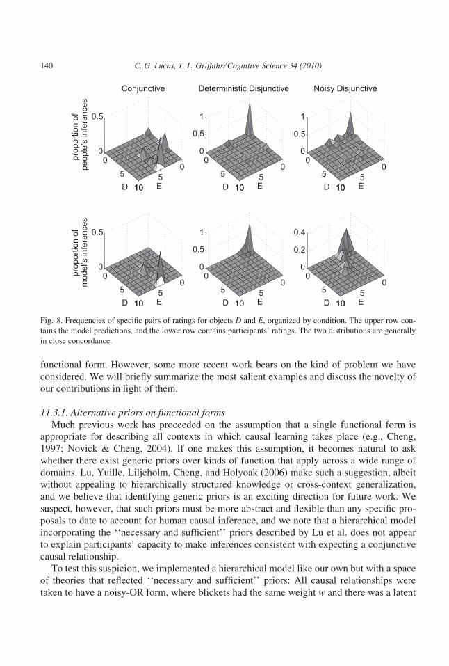
functional form. However, some more recent work bears on the kind of problem we have

considered. We will briefly summarize the most salient examples and discuss the novelty of

our contributions in light of them.

11.3.1. Alternative priors on functional formsMuch previous work has proceeded on the assumption that a single functional form is

appropriate for describing all contexts in which causal learning takes place (e.g., Cheng,

1997; Novick & Cheng, 2004). If one makes this assumption, it becomes natural to ask

whether there exist generic priors over kinds of function that apply across a wide range of

domains. Lu, Yuille, Liljeholm, Cheng, and Holyoak (2006) make such a suggestion, albeit

without appealing to hierarchically structured knowledge or cross-context generalization,

and we believe that identifying generic priors is an exciting direction for future work. We

suspect, however, that such priors must be more abstract and flexible than any specific pro-

posals to date to account for human causal inference, and we note that a hierarchical model

incorporating the ‘‘necessary and sufficient’’ priors described by Lu et al. does not appear

to explain participants’ capacity to make inferences consistent with expecting a conjunctive

causal relationship.

To test this suspicion, we implemented a hierarchical model like our own but with a space

of theories that reflected ‘‘necessary and sufficient’’ priors: All causal relationships were

taken to have a noisy-OR form, where blickets had the same weight w and there was a latent

Fig. 8. Frequencies of specific pairs of ratings for objects D and E, organized by condition. The upper row con-

tains the model predictions, and the lower row contains participants’ ratings. The two distributions are generally

in close concordance.


background cause with weight wn. The prior probability of a pair of weights was the same

as given in Lu et al.:

1

Z½e�aðwn�wÞ þ e�aðw�wnÞ�;

where Z is a normalizing constant. Once we optimized a, giving a ¼ 2.40, this model per-

formed much better than those that assume a fixed relationship, with an MSE of 0.71

(approximately twice the MSE resulting from using our sigmoid theory space). Nonetheless,

this model failed to make the key prediction that people would infer that two blickets were

necessary to activate the meter in the Experiment 2 conditions, leading us to conclude that

any psychologically real generic prior must be more flexible than these ‘‘necessary and suf-

ficient’’ priors.

11.4. Causal coherence

Lien and Cheng (2000) presented a theory explaining how people might identify the level

of generality at which causal inferences should be made and use that knowledge to aid later

inference. For example, in learning about the effects of a set of chemicals, one might either

infer a relationship between a specific chemical and an outcome, or form generalizations

about the effects of particular types of chemicals. There are some similarities between the

basic structure of their experimental design and our own that raise the question of how well

the notion of ‘‘causal coherence’’ they articulated might explain our results.

The basic argument in Lien and Cheng (2000) is that people learn what level of generality

is best for representing particular causal variables by selecting the best level from a set iden-

tified a priori, where the best level maximizes PðejcÞ � Pðej�cÞ, with c denoting a cause

identified at that level and e the effect. Lien and Cheng illustrate this idea with an example

using cigarettes and lung cancer: Given enough data, one could infer that lung cancer is

caused by (a) smoking particular brands of cigarettes, (b) smoking cigarettes, or (c) inhaling

any kind of fumes. Option (b) is preferable to (a) under the contrast criterion because

P(e|brand) � P(e|cigarettes) and P(e|brand) > P(e|cigarettes), and option (b) is preferable to

(c) under the assumption that ‘‘fumes’’ includes substances such that P(e|fumes) )P(e|fumes) < P(e|cigarettes) ) P(e|cigarettes).

While it does predict certain kinds of transfer of knowledge, such a theory cannot explain

our data: The only levels of generality our participants could have identified were specific

objects, ‘‘blickets’’ and ‘‘all objects,’’ and inference to any of these as causes leads to the

problems faced by any nonhierarchical model. A more general variation on the idea of

identifying the appropriate level of abstraction leads to the argument that a learner could use

preexisting domain knowledge to identify arbitrary events as prospective causes and use

the same contrast criterion to select amongst those. For instance, the ‘‘levels of abstraction’’

could include ‘‘one blicket,’’ ‘‘two blickets,’’ ‘‘one blicket and one nonblicket,’’ and so on

as possible causes. This might explain the results of Experiment 1, but more machinery is

necessary to explain the fact that participants concurrently learned causal structure and func-

tional form in Experiment 2. Moreover, this variation leads to so many possible causes that


a graded measure of plausibility is necessary along with a description of how that would

interact with contrast. We believe that filling these holes in a natural, parsimonious way

would lead to a model indistinguishable from a hierarchical Bayesian approach.

11.5. Other hierarchical Bayesian models

Other hierarchical Bayesian models of causal inference have been presented recently,

including one concerned with learning ‘‘causal schemata’’ (Kemp et al., 2007) and an

account of sequential causal learning (Lu, Rojas, et al., 2008). We would like to make clear

that our approach is not in competition with these. Rather, these perspectives are comple-

mentary. Kemp et al.’s contribution extends the infinite relational model (Kemp,

Tenenbaum, Griffiths, Yamada, & Ueda, 2006) to account for learning concurrently about

types and the causal relationships between them, but it makes no provision for flexibly

learning the form of causal relationships. Integrating a hierarchical representation of the

functional form with causal schemata would provide a natural answer to the question of

how people learn about functional form across diverse contexts.

Lu et al.’s (2008) sequential learning research touches on inferring the form of causal

relationships, but it commits to using two explicit forms—additive (linear sum) and subad-

ditive (noisy-MAX) functions for continuous variables—being largely concerned with

explaining the effects of presentation order. While their model cannot explain the range of

phenomena we have discussed, it nicely complements our focus on functional forms for bin-

ary variables. Taken together with the results we have presented in this paper, this work sug-

gests that a hierarchical Bayesian approach has the potential to provide a unifying

framework for explaining how people learn the functional form of causal relationships.

11.6. Toward a more general model of functional form learning

The specific hierarchical Bayesian model we used to generate quantitative predictions, in

which the set of possible functional forms is constrained to those that are consistent with the

logistic function, was motivated by its simplicity, flexibility, and consistency with the cover

stories that framed the evidence that participants saw in our experiments. While this model

was consistent with the judgments that participants made in these experiments, it was not

intended as a general account of how people learn the functional form of causal relation-

ships. In particular, it is inconsistent with functional forms that have previously been

explored in the causal learning literature, such as the experiment by Shanks and Darby

(1998) in which people learned that two causes produced an effect independently but not

when they occurred together.

The hierarchical Bayesian framework we have presented provides the basis for a more

general model of functional form learning, but it would need to be supplemented with a

richer set of theories concerning possible functional forms. The challenge in doing so lies in

defining a systematic way to specify these theories. One possibility is suggested by the

recent work of Yuille and Lu (2007), who showed that noisy-logical circuits consisting of

combinations of variables interacting through noisy-OR, noisy-AND, and negation opera-


tions could approximate any discrete probability distribution. This result suggests that

noisy-logical circuits might provide a reasonable foundation for characterizing a richer

hypothesis space of an functional forms, with the prior probability of a particular functional

form depending on the complexity of its expression in terms of these operations (for exam-

ples of this kind of an approach in categorization, see Feldman, 2000; Goodman, Tenen-

baum, Feldman, & Griffiths, 2008).

One important step toward understanding how people learn the functional form of causal

relationships more generally is identifying the prior probability assigned to different kinds

of relationships. The simple model we used in this paper made it possible to draw inferences

about this prior directly from people’s judgments, through the parameter kb and kg. Identify-

ing priors over richer sets of functions poses more of a challenge and will require experi-

ments investigating the difficulty that people encounter in learning functions of different

forms. We are currently conducting experiments looking at a wider range of functional

forms, and exploring the possibility of using a probabilistic logic to capture the human abil-

ity to make inferences consistent with a wide range of functional forms while still exploiting

prior knowledge, as in the cases we consider here.

12. Conclusion

The results of our experiments show that people efficiently learn about the functional

forms of causal relationships using covariation data, category information, and verbal cues,

making judgments that are accurately predicted by a hierarchical Bayesian model. These

results are compatible with earlier experimental results suggesting that people are sensitive

to causal mechanisms and with developmental theories about domain knowledge and frame-

work theories, but they are not predicted by most existing models of covariation-based cau-

sal inference. The Bayesian approach we have taken in this paper is capable of explaining

not just how knowledge of causal mechanisms should influence causal inference, but how

that knowledge could itself be acquired.

If human causal inference is tightly coupled to abstract knowledge, then some questions

remain to be answered. How flexible is this knowledge? Do we possess general inductive

mechanisms that permit us to learn a broader set of kinds of causal relationships than are

common in the world given sufficient evidence, or do we operate under tight constraints?

Where does abstract knowledge about categories and properties intersect with causal infer-

ence? Work along these lines is in progress and we ultimately hope to begin to chart both

the structure of adults’ causal theories and the developmental trajectory of the acquisition of

this knowledge.

Notes

1. Nothing prevents constraint-based approaches from including assumptions about func-

tional form to facilitate rapid learning—in such cases one would test specific classes


of relationships reflecting the assumptions rather than general statistical indepen-

dence—but such assumptions lead to the same restrictions that face other fixed-form

models.

2. A note on terminology: We have chosen to use the terms disjunctive and conjunctiveinstead of, for example, OR and Noisy-AND, in the interest of accuracy. A disjunctive(generative) causal relationship is one in which the probability of the effect increases

at most linearly with the number of causes present, and a conjunctive relationship is

one in which the probability effect increases more sharply once some number of

causes (n > 1) is exceeded. Noisy-OR and noisy-AND functions are special cases of

these and are used where appropriate.

3. Previous work using a similar device has referred to it as a ‘‘blicket machine’’ or

‘‘blicket detector’’ (Gopnik & Sobel, 2000; Sobel, Tenenbaum, & Gopnik, 2004). We

chose to call it a ‘‘blicketosity meter’’ as this gave minimal cues to functional form,

while ‘‘blicket detector’’ seems more consistent with an OR function.

4. We will represent events as a set of present or active prospective causes and the presence

or absence of an effect, for example, if possible causes A and B are present and the effect

is observed, the event can be written down as ({a,b},e) or, more concisely, as AB+.

5. Based on the suspicion that people would strongly favor deterministic functions, we

considered using an inverse-exponential prior for the steepness—which assigns very

low probability to values near zero—but abandoned it in favor of the exponential

which can also strongly favor deterministic theories with the right parameter and is

compatible with a wider range of beliefs, such as that the meter is acting randomly.

6. Hypothetically, a noisy-disjunctive relationship with a high failure rate coupled with a

belief that almost all objects are blickets could lead to such an inference, but such an

explanation is incompatible with ratings participants gave for E.

Acknowledgments

We are grateful for support from the James S. McDonnell Foundation’s Causal Learning

Initiative and grant number FA9550-07-1-0351 from the Air Force Office of Scientific

Research. We thank David Danks and two anonymous reviewers for their helpful comments

and suggestions regarding this research, parts of which were presented at the 41st Annual

Meeting of the Society for Mathematical Psychology and the 30th Annual Meeting of the

Cognitive Science Society.

References

Ahn, W., Kalish, C. W., Medin, D. L., & Gelman, S. A. (1995). The role of covariation versus mechanism

information in causal attribution. Cognition, 54, 299–352.

Alloy, L. B., & Tabachnik, N. (1984). Assessment of covariation by humans and animals: The joint influence of

prior expectations and current situational information. Psychological Review, 91, 112–149.


Anderson, J. R. (1990). The adaptive character of thought. Hillsdale, NJ: Erlbaum.

Beckers, T., De Houwer, J., Pineno, O., & Miller, R. R. (2005). Outcome additivity and outcome maximality

influence cue competition in human causal learning. Journal of Experimental Psychology: Learning,Memory, and Cognition, 31(2), 238–249.

Bullock, M., Gelman, R., & Baillargeon, R. (1982). The development of causal reasoning. In W. J. Friedman

(Ed.), The developmental psychology of time (pp. 209–254). New York: Academic Press.

Carey, S. (1991). Knowledge acquisition: Enrichment or conceptual change? In S. Carey & R. Gelman

(Eds.), The epigenesis of mind: Essays on biology and cognition (pp. 257–292). Hillsdale, NJ: Erlbaum

Associates.

Cheng, P. (1997). From covariation to causation: A causal power theory. Psychological Review, 104, 367–405.

Cooper, G., & Herskovits, E. (1992). A Bayesian method for the induction of probabilistic networks from data.

Machine Learning, 9, 308–347.

Estes, W. (1956). The problem of inference from curves based on group data. Psychological Bulletin, 53(2),

134–140.

Feldman, J. (2000). Minimization of Boolean complexity in human concept learning. Nature, 407, 630–633.

Gelman, A., Carlin, J. B., Stern, H. S., & Rubin, D. B. (1995). Bayesian data analysis. New York: Chapman &

Hall.

Glymour, C. (1998). Learning causes: Psychological explanations of causal explanation. Minds and Machines,

8, 39–60.

Goodman, N. D., Tenenbaum, J. B., Feldman, J., & Griffiths, T. L. (2008). A rational analysis of rule–based

concept learning. Cognitive Science, 32, 108–154.

Gopnik, A., & Sobel, D. (2000). Detecting blickets: How young children use information about novel causal

powers in categorization and induction. Child Development, 71, 1205–1222.

Gopnik, A., & Wellman, H. (1992). Why the child’s theory of mind really is a theory. Mind and Language, 7,

145–171.

Griffiths, T. L. (2005). Causes, coincidences, and theories. Unpublished doctoral dissertation, Stanford Univer-

sity.

Griffiths, T. L., & Tenenbaum, J. B. (2005). Structure and strength in causal induction. Cognitive Psychology,

51, 354–384.

Griffiths, T. L., & Tenenbaum, J. B. (2007). Two proposals for causal grammars. In A. Gopnik & L. E. Schulz

(Eds.), Causal learning: Psychology, philosophy, and computation (pp. 323–346). Oxford, England: Oxford

University Press.

Hume, D. (1748). An enquiry concerning human understanding. Indianapolis, IN: Hackett.

Jenkins, H. M., & Ward, W. C. (1965). Judgment of contingency between responses and outcomes. Psychologi-cal Monographs, 79, 1–17.

Kemp, C., Goodman, N. D., & Tenenbaum, J. B. (2007). Learning causal schemata. In Proceedings of the 29thAnnual Conference of the cognitive science society (pp. 389–394). Mahwah, NJ: Erlbaum.

Kemp, C., Tenenbaum, J. B., Griffiths, T. L., Yamada, T., & Ueda, N. (2006). Learning systems of concepts with

an infinite relational model. In 21st national conference on artificial Intelligence). Menlo Park, CA: AAAI

Press.

Koslowski, B. (1996). Theory and evidence: The development of scientific reasoning. Cambridge, MA: MIT

Press.

Lien, Y., & Cheng, P. W. (2000). Distinguishing genuine from spurious causes: A coherence hypothesis. Cogni-tive Psychology, 40, 87–137.

Lu, H., Rojas, R. R., Beckers, T., & Yuille, A. (2007). Sequential causal learning in humans and rats.

In D. McNamara & G. Trafton (Eds.), Proceedings of the 29th annual conference of the cognitive sciencesociety (pp. 185–188). Mahwah, NJ: Erlbaum.

Lu, H., Yuille, A., Liljeholm, M., Cheng, P. W., & Holyoak, K. J. (2006). Modeling causal learning using Bayes-

ian generic priors on generative and preventive powers. In R. Sun & N. Miyake (Eds.), Proceedings of the28th conference of the cognitive science society (pp. 519–524). Hillsdale, NJ: Erlbaum.


Lu, H., Yuille, A., Liljeholm, M., Cheng, P. W., & Holyoak, K. J. (2007). Bayesian models of judgments of

causal strength: A comparison. In D. S. McNamara & G. Trafton (Eds.), Proceedings of the 29th annualconference of the cognitive science society (pp. 1241–1246). Mahwah, NJ: Erlbaum.

Lu, H., Yuille, A. L., Liljeholm, M., Cheng, P. W., & Holyoak, K. J. (2008). Bayesian generic priors for causal

learning. Psychological Review, 115(4), 955–984.

Marr, D. (1982). Vision. San Francisco: W.H. Freeman.

Myung, I. J., Kim, C., & Pitt, M. A. (2000). Toward an explanation of the power law artifact: Insights from

response surface analysis. Memory & Cognition, 28(5), 832–840.

Navarro, D. J., Griffiths, T. L., Steyvers, M., & Lee, M. D. (2006). Modeling individual differences using Dirich-

let processes. Journal of Mathematical Psychology, 50, 101–122.

Novick, L. R., & Cheng, P. W. (2004). Assessing interactive causal influence. Psychological Review, 111, 455–

485.

Pearl, J. (1988). Probabilistic reasoning in intelligent systems. San Francisco: Morgan Kaufmann.

Pearl, J. (2000). Causality: Models, reasoning and inference. Cambridge, England: Cambridge University Press.

Perales, J. C., & Shanks, D. R. (2007). Models of covariation-based causal judgment: A review and synthesis.

Psychonomic Bulletin and Review, 14(4), 577–596.

Rescorla, R. A., & Wagner, A. R. (1972). A theory of Pavlovian conditioning: Variations on the effectiveness of

reinforcement and non-reinforcement. In A. H. Black & W. F. Prokasy (Eds.), Classical conditioning II:Current research and theory (pp. 64–99). New York: Appleton-Century-Crofts.

Schulz, L., & Sommerville, J. (2006). God does not play dice: Causal determinism and preschoolers causal

inferences. Child Development, 77(2), 427–442.

Shanks, D. R. (1995). The psychology of associative learning. Cambridge, England: Cambridge University

Press.

Shanks, D. R., & Darby, R. J. (1998). Feature- and rule-based generalization in human associative learning.

Journal of Experimental Psychology: Animal Behavior Processes, 24(4), 405–415.

Shultz, T. R. (1982). Rules of causal attribution. Monographs of the Society for Research in Child Development,47(Serial no. 194), 1–51.

Sobel, D. M., Tenenbaum, J. B., & Gopnik, A. (2004). Children’s causal inferences from indirect evidence:

Backwards blocking and Bayesian reasoning in preschoolers. Cognitive Science, 28, 303–333.

Spirtes, P., Glymour, C., & Schienes, R. (1993). Causation prediction and search. New York: Springer-Verlag.

Tenenbaum, J. B., & Griffiths, T. L. (2001). Structure learning in human causal induction. In T. Leen, T. Dietterich,

& V. Tresp (Eds.), Advances in neural information processing systems 13 (pp. 59–65). Cambridge, MA: MIT

Press.

Tenenbaum, J. B., & Griffiths, T. L. (2003). Theory–based causal induction. In S. Becker, S. Thrun, & K. Ober-

mayer (Eds.), Advances in neural information processing systems 15 (pp. 35–42). Cambridge, MA: MIT

Press.

Tenenbaum, J. B., & Niyogi, S. (2003). Learning causal laws. In R. Alterman & D. Kirsh (Eds.), Proceedings ofthe 25th annual meeting of the cognitive science society (pp. 1152–1157). Hillsdale, NJ: Erlbaum.

Vul, E., & Pashler, H. (2008). Measuring the crowd within: Probabilistic representations within individuals.

Psychological Science, 19(7), 645–647.

Waldmann, M. R. (1996). Knowledge–based causal induction. In D. Shanks, K. Holyoak & D. Medin (Eds.),

The psychology of learning and motivation (Vol. 34, pp. 47–88). San Diego, CA: Academic Press.

Waldmann, M. R. (2007). Combining versus analyzing multiple causes: How domain assumptions and task

context affect integration rules. Cognitive Science, 31, 233–256.

Yuille, A. L., & Lu, H. (2007). The noisy–logical distribution and its application to causal inference. In J. C.

Platt, D. Koller, Y. Singer & S. Rowets (Eds.), Advances in neural information processing systems 20(pp. 449–456). Cambridge, MA: MIT Press.

Zelazo, P. R., & Shultz, T. R. (1989). Concepts of potency and resistance in causal prediction. ChildDevelopment, 60, 1307–1315.


Appendix: Materials for Experiment 5

The cover story for the dax blocks:

You will read about some rodents. Your goal is to figure out which of them are

Daxes—some are and some are not. People cannot tell Daxes from non-Daxes, but cats can

smell Daxes and are afraid of them. There are three rodents, called A, B, and C. The list

below describes what happened when a cat was exposed to different rodents or groups of

rodents.

The training block evidence in the Dax condition:

One time, the cat was exposed to A. The cat did not run away.

Another time, the cat was exposed to B. The cat did not run away.

Another time, the cat was exposed to C. The cat did not run away.

Another time, the cat was exposed to A and B. The cat did not run away.

Another time, the cat was exposed to A and C. The cat ran away.

Another time, the cat was exposed to B and C. The cat did not run away.

The questions people were asked in the Dax-condition training block:

Write down for rodents A, B, and C the probability that each is a Dax, using a number

from 0 to 10 where 0 means you are absolutely certain it is not a Dax, 10 means you are

absolutely certain it is a Dax, and 5 means it is equally likely to be a Dax as not.

Test block materials differed only in the specific evidence given.


learning the form of causal relationships using

Documents