learning the virtual work method in statics: what is a ... · learning the virtual work method in...

2006-823: LEARNING THE VIRTUAL WORK METHOD IN STATICS: WHAT IS ACOMPATIBLE VIRTUAL DISPLACEMENT?

Ing-Chang Jong, University of ArkansasIng-Chang Jong serves as Professor of Mechanical Engineering at the University of Arkansas. Hereceived a BSCE in 1961 from the National Taiwan University, an MSCE in 1963 from SouthDakota School of Mines and Technology, and a Ph.D. in Theoretical and Applied Mechanics in1965 from Northwestern University. He was Chair of the Mechanics Division, ASEE, in 1996-97.His research interests are in mechanics and engineering education.

© American Society for Engineering Education, 2006

1.878.1

Learning the Virtual Work Method in Statics:

What Is a Compatible Virtual Displacement?

Abstract

Statics is a course aimed at developing in students the concepts and skills related to the analysis

and prediction of conditions of bodies under the action of balanced force systems. At a number

of institutions, learning the traditional approach using force and moment equilibrium equations is

followed by learning the energy approach using the virtual work method to enrich the learning of

students. The transition from the traditional approach to the energy approach requires learning

several related key concepts and strategy. Among others, compatible virtual displacement is a

key concept, which is compatible with what is required in the virtual work method but is not

commonly recognized and emphasized. The virtual work method is initially not easy to learn for

many people. It is surmountable when one understands the following: (a) the proper steps and

strategy in the method, (b) the displacement center, (c) some basic geometry, and (d ) the radian

measure formula to compute virtual displacements. For learning and pedagogical purposes, this

paper includes seven examples with various levels of challenge.

I. Introduction

More often than not, it is manifested that the virtual work method is used to treat problems in-

volving mainly machines. This manifestation comes about as a consequence of focusing on the

determination of the equilibrium configuration of a series of pin-connected members by restrict-

ing virtual displacements to be consistent with constraints at the supports. In general, such a re-

striction is too strong and is an over restriction. It prevents the virtual work method from being

effectively used to treat problems involving beams and frames, and it diminishes the usefulness

of the virtual work method in Statics. As a result, some feel that the virtual work method lacks

broad appeal in Statics. Nonetheless, the virtual work method is a standing topic contained in

most textbooks of Statics. By and large, such a topic is covered in Statics at the discretion of the

instructors to enrich the learning of students.

Both the traditional method and the virtual work method equally require and emphasize the

drawing of free-body diagrams, although the former involves more algebra and the latter uses

more geometry in solving problems. Most students find that learning the virtual work method is

challenging, since they are generally better at algebra than geometry. It is not the intent of this

paper to urge anyone to teach the virtual work method or to upstage the time-honored traditional

method in Statics. Rather, this paper is mainly aimed at being an extension to previous efforts1-9

of mechanics educators and textbook authors who included the virtual work method in Statics. In

particular, this paper identifies key concepts, steps, and strategy that have been helpful to stu-

dents in learning the virtual work method. Readers, who are familiar with this method, may skip

the refresher on the rudiments included in the early part of this paper.

A displacement of a body is a change of position of the body. A rigid-body displacement of a

body is a change of position of the body without inducing any strain in the body. A virtual dis-

Page 11.878.2

placement of a body is an imaginary, first-order differential displacement, which is possible but

does not actually take place. A rigid-body virtual displacement of a body is a rigid-body dis-

placement as well as a virtual displacement of the body, where the body undergoes an imaginary,

first-order differential deflection to a neighboring position without experiencing any strain.

Work is energy in transition to a system due to force or moment acting on the system during a

displacement of the system. Heat is energy in transition to a system due to temperature differ-

ence between the system and its surroundings. Work, as well as heat, is dependent on the path of

a process. Like heat, work crosses the system boundary when the system undergoes a process.

Unlike kinetic energy and potential energy, work is not a property possessed by a system. In me-

chanics, a body receives work from a force or a moment that acts on it while it undergoes a dis-

placement in the direction of the force or moment, respectively, during the action. It is the force

or moment, rather than the body, which does work. A virtual work is the work done by force or

moment during a virtual displacement of the body.

Fig. 1 Compatible virtual displacement of body AB to position A B| |

In virtual work method, compatible virtual displacements (besides rigid-body virtual displace-

ments) are to be used, where second-order (not first-order) straining of members in a system is

permitted in drawing virtual displacement diagrams. This may initially come across as being

against the grain of the usual mentality of rigid bodies held for Statics. Notwithstanding, a work-

ing definition is in order. As shown in Fig. 1, a compatible virtual displacement of a body AB

is an imaginary displacement resulting from a first-order differential angular displacement fs of

the body about a certain point D, called its displacement center,6,7

during which the body de-

flects from position AB to another position A B| | and the following conditions exist

AA AD| ` BB BD| ` A B AB| | ‡

The displacement vectors AA|iiif

and BB|iiif

in Fig. 1 are called the compatible virtual displacements

of points A and B, respectively.

The concept of compatible virtual displacement is compatible with what is required in the virtual

work method, and it is a critical one in teaching and learning the virtual work method. Note that

this concept has a subtle shade of difference from the traditional concept of rigid-body virtual

displacement defined earlier.

Page 11.878.3

II. Rigid-Body versus Compatible Virtual Displacements

All bodies considered in this paper are rigid bodies or systems of pin-connected rigid bodies,

where the pins are taken as frictionless and no resisting moments are developed in the joints. If a

body AB undergoes a rigid-body virtual displacement by rotating about its end A, as its dis-

placement center, through an angular displacement fs , it will experience no axial strain to reach

the position AB|| , not AB| , as illustrated in Fig. 2. However, if the body AB undergoes a com-

patible virtual displacement by rotating about its end A, as its displacement center, through an

angular displacement fs , it will experience some axial strain to reach the position AB| , not

AB|| , as illustrated in Fig. 2.

Fig. 2 Rigid-body versus compatible virtual displacements of body AB

Using series expansion in terms of the first-order differential angular displacement fs, which is

infinitesimal, we find that the difference between AB| and AB|| is given by

2 4 65 611

2 24 720sec 1 ( ) ( ) ( )B B L L L Lfs fs fs fs|| | Ç ×? / ? - - - - ©© © /É Ú

^ 2

2( )LB B fs|| | … + higher order terms of fs (1)

Since fs"is infinitesimally small, the amount of axial strain experienced by body AB is

2

1 22

2

( )( )

LB B

LAB

fsg fs|| |? … ? (2)

Thus, in undergoing compatible virtual displacement from position AB to position AB| , the body

AB may, at most, experience an axial strain of the second order of fs. Meanwhile, the compati-

ble virtual displacement of point B in Fig. 2 is the displacement vector from B to . The magni-

tude of this displacement vector is

|B

3 5 7171 2

3 15 315tan ( ) ( ) ( )BB L L Lfs fs fs fs fs f| Ç ×? ? - - - - ©© © …É Ú s (3)

In Fig. 2, the lengths of the chord |BB and the arc fl||BB can be taken as equal as 0fs › in the

limit. Equation (3) shows that the magnitude of the compatible virtual displacement of point B

may indeed be computed by using the radian measure formula in calculus; i.e.,

s?s r (4)

where s is the arc subtending an angle s (in radians) included by two radii of length r. Note that

Eq. (4) is extremely useful and important in solving problems by the virtual work method!

Page 11.878.4

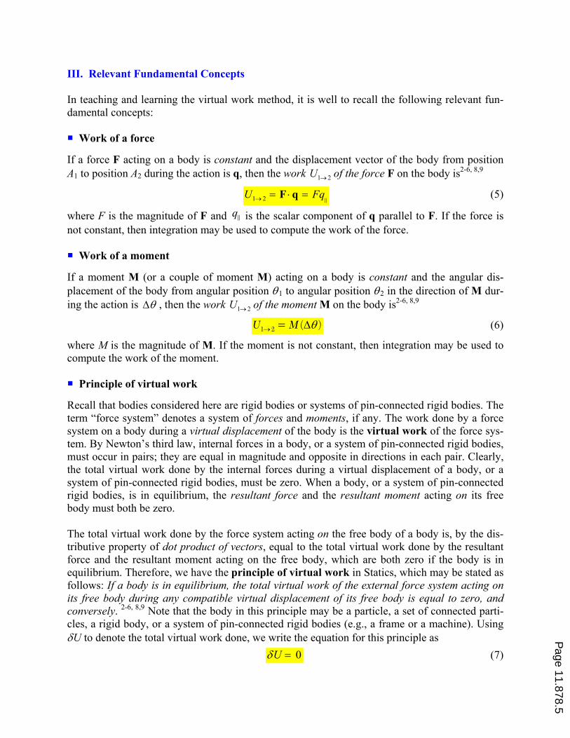
III. Relevant Fundamental Concepts

In teaching and learning the virtual work method, it is well to recall the following relevant fun-

damental concepts:

Work of a force

If a force F acting on a body is constant and the displacement vector of the body from position

A1 to position A2 during the action is q, then the work of the force F on the body is1 2U ›2-6, 8,9

1 2U › Fq? © ?F qE (5)

where F is the magnitude of F and q is the scalar component of q parallel to F. If the force is

not constant, then integration may be used to compute the work of the force.

E

Work of a moment

If a moment M (or a couple of moment M) acting on a body is constant and the angular dis-

placement of the body from angular position s1 to angular position s2 in the direction of M dur-

ing the action is sF , then the work of the moment M on the body is1 2U ›2-6, 8,9

s› F?1 2 (U M ) (6)

where M is the magnitude of M. If the moment is not constant, then integration may be used to

compute the work of the moment.

Principle of virtual work

Recall that bodies considered here are rigid bodies or systems of pin-connected rigid bodies. The

term “force system” denotes a system of forces and moments, if any. The work done by a force

system on a body during a virtual displacement of the body is the virtual work of the force sys-

tem. By Newton’s third law, internal forces in a body, or a system of pin-connected rigid bodies,

must occur in pairs; they are equal in magnitude and opposite in directions in each pair. Clearly,

the total virtual work done by the internal forces during a virtual displacement of a body, or a

system of pin-connected rigid bodies, must be zero. When a body, or a system of pin-connected

rigid bodies, is in equilibrium, the resultant force and the resultant moment acting on its free

body must both be zero.

The total virtual work done by the force system acting on the free body of a body is, by the dis-

tributive property of dot product of vectors, equal to the total virtual work done by the resultant

force and the resultant moment acting on the free body, which are both zero if the body is in

equilibrium. Therefore, we have the principle of virtual work in Statics, which may be stated as

follows: If a body is in equilibrium, the total virtual work of the external force system acting on

its free body during any compatible virtual displacement of its free body is equal to zero, and

conversely. 2-6, 8,9

Note that the body in this principle may be a particle, a set of connected parti-

cles, a rigid body, or a system of pin-connected rigid bodies (e.g., a frame or a machine). Using

fU to denote the total virtual work done, we write the equation for this principle as

0f ?U (7)

Page 11.878.5

Conventional method versus virtual work method

With the conventional method, equilibrium problems are solved by applying two basic equilib-

rium equations: (a) force equilibrium equation, and (b) moment equilibrium equation; i.e.,

U ?F 0 (8)

U ?P

M 0 (9)

With the virtual work method, equilibrium problems are solved by applying the virtual work

equation, which sets to zero the total virtual work fU done by the force system on the free body

during a chosen compatible virtual displacement of the free body; i.e.,

0f ?U (Repeated) (7)

IV. Learning the Virtual Work Method: Examples

There are three major steps and one strategy in using the virtual work method. Step 1: Draw

the free-body diagram (FBD). Step 2: Draw the virtual-displacement diagram (VDD) with a

strategy. Step 3: Set to zero the total virtual work done. The strategy in step 2 is to give the free

body a compatible virtual displacement in such a way that only the unknown to be determined,

besides the applied loads that are already known, will be involved in the total virtual work done.

This strategy is the key to successful solutions of problems using the virtual work method. It is

important to understand and master this strategy before attempting to solve any problem.

In a nutshell, the virtual work method simply consists of three major steps and one strategy! To

be more helpful to those who wish to compare the features between the virtual work method and

the traditional method, the following seven illustrative examples are chosen for pedagogical pur-

poses and are arranged in increasing level of challenge. In particular, Example 1 presents a paral-

lel comparison between the traditional method and the virtual work method. Naturally, teaching

of the virtual work method in Statics is usually aimed at enriching the learning of students as cir-

cumstances warrant.

Example 1. Determine the vertical reaction force By at the roller support B of the simple beam

loaded as shown in Fig. 3 by using (a) the traditional method, and (b) the virtual work method.

Fig. 3 A simple beam carrying an inclined concentrated load

Solution. Note that color codes are here employed in the solution to enhance head-to-head com-

parison of (a) the traditional method, and (b) the virtual work method.

(a) Traditional method to solve for By: It is a usual procedure in the traditional method to first

draw the FBD of the beam as shown in Fig. 4.

Page 11.878.6

Fig. 4 Free-body diagram (FBD) for the simple beam

Next, we refer to the FBD in Fig. 4 and apply Eq. (9) to write

+S"UMA = 0: 4

53 (600) 5 0( ) yB/ - ?

^ By = 288 288 N y ? ‹B

(b) Virtual work method to solve for By: We shall follow the steps and strategy as outlined.

Step 1: We draw the FBD for the beam as shown in Fig. 4.

Fig. 4 FBD for the simple beam (Repeated)

Step 2: Keeping an eye on the FBD in Fig. 4, we draw a VDD for the beam with a strategy as

shown in Fig. 5, where we let the beam rotate counterclockwise through an imaginary angular

displacement fs about point A as the displacement center, and we have applied Eq. (4), the ra-

dian measure formula, in labeling the magnitudes of the virtual displacements of points C and B

as follows:

3CC fs| ? 5BB fs| ?

Fig. 5 Virtual-displacement diagram (VDD) for determining only By

The resulting VDD is well done because it will allow no unknowns except By to be involved in

the total virtual work done.

Step 3: We refer to Figs. 4 and 5 and apply Eqs. (5) and (7) to write

fU = 0: 4

5(600)( 3 ) (5 ) 0yBfs fs/ - ?

^ By = 288 288 N y ? ‹B

Remarks. We see in Example 1 that both the traditional method and the virtual work method

can solve the same simple problem and arrive at the same solution. Although using the virtual

work method to solve a simple problem may appear “unconventional,” we shall see that this

method has more advantage in solving more challenging problems, such as those shown below.

Page 11.878.7

Example 2. A combined beam (a Gerber beam) is loaded as shown in Fig. 6. Using the virtual

work method, determine only the reaction moment MA at the fixed support A.

Fig. 6 A combined beam with hinge connections at B, D, and G

Solution. We shall follow the outlined steps and strategy in the method to directly solve for MA.

Step 1: We draw the FBD for the combined beam as shown in Fig. 7.

Fig. 7 FBD for the combined beam

Step 2: Keeping an eye on the FBD in Fig. 7 and applying Eq. (4), we draw a VDD for the beam

with a strategy as shown in Fig. 8. Note that we let member AB rotate about A through an imagi-

nary angle fs S to get a compatible virtual displacement of the beam as shown, where the mem-

bers DEFG and GHI are unmoved according to the strategy. The resulting VDD is well done

because it will allow no unknowns except MA to be involved in the total virtual work done.

Fig. 8 VDD for determining only MA

Step 3: We refer to Figs. 7 and 8 and apply Eqs. (5), (6), and (7) to write

fU = 0: ( ) 500( 4 ) 600( ) 0AM fs fs fs- / - ? 1400AM ? 1400 lb ft A ? ©M S

Remarks. If we are to use the traditional method, we refer to the FBD in Fig. 7 and write

„ At hinge B, MB = 0: 4A yM A 0/ ? (i)

„ At hinge D, MD = 0: 8 4(500) 600 0yAM A/ - / ? (ii)

These two simultaneous equations yield: Ay = 350 and MA = 1400.

Thus, the traditional method confirms the same solution: 1400 lb ft A ? ©M S

Page 11.878.8

Example 3. A combined beam is loaded as shown in Fig. 6. Using the virtual work method, de-

termine only the vertical reaction force Ay at the fixed support A.

Fig. 6 A combined beam with hinge connections at B, D, and G (Repeated)

Solution. We shall follow the outlined steps and strategy in the method to directly solve for Ay.


Fig. 7 FBD for the combined beam (Repeated)


with a strategy as shown in Fig. 9, where we let member BCD rotate about D through an imagi-

nary angle fs R to get a compatible virtual displacement of the beam as shown, where the

members DEFG and GHI are unmoved according to the strategy. The resulting VDD is well

done because it will allow no unknowns except Ay to be involved in the total virtual work done.

Fig. 9 VDD for determining only Ay


fU = 0: (4 ) 500( 4 ) 600( ) 0yA fs fs fs- / - ? 350yA ? 350 lb y ? ‹A




These two simultaneous equations yield: Ay = 350 and MA = 1400.

Thus, the traditional method confirms the same solution: 350 lb y ? ‹A

Page 11.878.9


termine only the vertical reaction force at the roller support E. yE


Solution. We shall follow the outlined steps and strategy in the method to directly solve for Ey.




with a strategy as shown in Fig. 10, where we let member DEFG rotate about G through an

imaginary angle fs R to get a compatible virtual displacement of the beam as shown. Members

AB and GHI are unmoved according to the strategy. The resulting VDD is well done because it

will allow no unknowns except to be involved in the total virtual work done. yE

Fig. 10 VDD for determining only Ey


fU = 0: 4

5600( 2.5 ) (6 ) (1500)( 4 ) 0yEfs fs fs/ - - / ? 1050yE ? 1050 lb y ? ‹E




„ At hinge G, MG = 0: 4

518 14 (500) 600 6 4 (1500) 0( )y yAM A E/ - / / - ? (iii)

These three simultaneous equations yield: Ay = 350, MA = 1400, and Ey = 1050.

Thus, the traditional method confirms the same solution: 1050 lb y ? ‹E

Page 11.878.10


termine only the vertical reaction force at the roller support H. yH


Solution. We shall follow the outlined steps and strategy in the method to directly solve for Hy.




with a strategy as shown in Fig. 11, where we let member BCD rotate about B through an

imaginary angle fs R and unmoved points E and I to get a compatible virtual displacement of

the beam as shown. Member AB is, by strategy, unmoved. The resulting VDD is well done be-

cause it will allow no unknowns except to be involved in the total virtual work done. yH

Fig. 11 VDD for determining only Hy


fU = 0: 4

5600( ) (1500)( 2 ) 200( 6 ) (4 ) 0yHfs fs fs fs- / - / - ? 750yH ? 750 lb y ? ‹H


„ At hinge G, MG = 0: (i) 6 2y yI H/ - ? 0

„ At hinge D, MD = 0: 4

516 12 10(200) 6 (1500) 4 0( )y y yI H E/ - / / - ? (ii)

„ At hinge B, MB = 0: 4

520 16 14(200) 10 (1500) 8 600 0( )y y yI H E/ - / / - / ? (iii)

These three simultaneous equations yield: Ey = 1050, Hy = 750, and Iy = 250.

Thus, the traditional method confirms the same solution: 750 lb y ? ‹H

.878.11

Example 6. A frame is loaded as shown in Fig. 12. Using the virtual work method, determine

only the reaction moment MA at the fixed support A.

Fig. 12 A frame with a fixed support at A and a hinge support at D

Solution. We shall follow the outlined steps and strategy in the method to directly solve for MA.

Step 1: We draw the FBD for the frame as shown in Fig. 13.

Fig. 13 FBD for the frame Fig. 14 VDD for determining only MA

Step 2: Keeping an eye on the FBD in Fig. 13 and applying Eq. (4), we draw a VDD for the

frame with a strategy as shown in Fig. 14, where we let member DEF rotate about D through an

imaginary angle fs S and unmoved points A and D. The resulting VDD is well done because it

will allow no unknowns except MA to be involved in the total virtual work done.


fU = 0: ( 2 ) 6(12 ) 2( 4 ) 10 0AM fs fs fs fs/ - - / - ? 37AM ? 37 kN m A ? ©M S


„ At pin B of member ABC, MB = 0: 2 4(6) 0xAM A- / ? (i)

„ At pin E of members BGE & ABC, ME = 0: 2 6 4(6) 3(4) 0yA xM A A- / / - ? (ii)

„ For entire frame, +S"UMD = 0: 6 6 3(4) 10 4(2) 0x yAM A A- / - - / ? (iii)

These three simultaneous equations yield: Ax = &6.5, Ay = 2, and MA = 37.

Thus, the traditional method confirms the same solution: 37 kN m A ? ©M S

Page 11.878.12

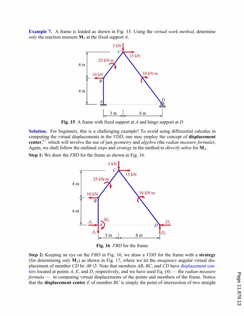
Example 7. A frame is loaded as shown in Fig. 15. Using the virtual work method, determine

only the reaction moment MA at the fixed support A.

Fig. 15 A frame with fixed support at A and hinge support at D

Solution. For beginners, this is a challenging example! To avoid using differential calculus in

computing the virtual displacements in the VDD, one may employ the concept of displacement

center,6,7

which will involve the use of just geometry and algebra (the radian measure formula).

Again, we shall follow the outlined steps and strategy in the method to directly solve for MA.

Step 1: We draw the FBD for the frame as shown in Fig. 16.

Fig. 16 FBD for the frame

Step 2: Keeping an eye on the FBD in Fig. 16, we draw a VDD for the frame with a strategy

(for determining only MA) as shown in Fig. 17, where we let the imaginary angular virtual dis-

placement of member CD be fs S. Note that members AB, BC, and CD have displacement cen-

ters located at points A, E, and D, respectively, and we have used Eq. (4) — the radian measure

formula — in computing virtual displacements of the points and members of the frame. Notice

that the displacement center E of member BC is simply the point of intersection of two straight

Page 11.878.13

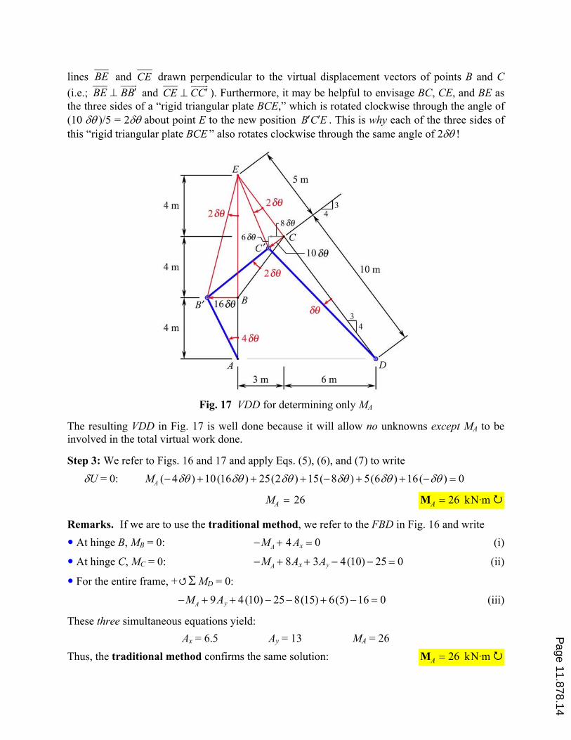
lines BE and CE drawn perpendicular to the virtual displacement vectors of points B and C

(i.e.; BE BB|`iiif

and CE CC|`iiif

). Furthermore, it may be helpful to envisage BC, CE, and BE as

the three sides of a “rigid triangular plate BCE,” which is rotated clockwise through the angle of

(10 fs )/5 = 2fs about point E to the new position B C E| | . This is why each of the three sides of

this “rigid triangular plate BCE ” also rotates clockwise through the same angle of 2fs !

Fig. 17 VDD for determining only MA

The resulting VDD in Fig. 17 is well done because it will allow no unknowns except MA to be

involved in the total virtual work done.


" fU = 0: ( 4 ) 10(16 ) 25(2 ) 15( 8 ) 5(6 ) 16( ) 0AM fs fs fs fs fs fs/ - - - / - - / ?

26AM ? 26 kN·m A ?M R "


„ At hinge B, MB = 0: 4 0A xM A/ - ? (i)

„ At hinge C, MC = 0: 8 3 4(10) 25 0yA xM A A/ - - / / ? (ii)

„ For the entire frame, +S"UMD = 0:

(iii) 9 4(10) 25 8(15) 6(5) 16 0yAM A/ - - / / - / ?

These three simultaneous equations yield:

Ax = 6.5 Ay = 13 MA = 26

Thus, the traditional method confirms the same solution: 26 kN·m A ?M R

Page 11.878.14

V. Concluding Remarks

Oftentimes, the virtual work method is used to treat problems involving mainly machines, where

virtual displacements are restricted to be consistent with constraints at the supports. Such a re-

striction is generally too strong and is an over restriction in treating other types of problems. In

particular, it prevents the virtual work method from being effectively used to treat problems in-

volving beams and frames, and it diminishes the usefulness of the virtual work method in Statics.

The subtle shade of difference between a compatible virtual displacement and a rigid-body

virtual displacement is pointed out in the presentation, although it has not been commonly rec-

ognized and emphasized in the literature. In using the virtual work method to solve problems in-

volving beams, frames, or machines, we need to remember that all compatible virtual displace-

ments are acceptable virtual displacements. There are three major steps and one strategy in the

virtual work method.

Solving a simple equilibrium problem by the virtual work method may come across as “uncon-

ventional” or “an act of overkill,” as witnessed in Example 1. Still, the virtual work method is a

standing topic in Statics, and it has been shown to have advantages in solving challenging prob-

lems as illustrated in Examples 2 through 7. Naturally, teaching of such a topic in Statics is usu-

ally at the discretion of the instructors to enrich the learning of students. It may be true that the

virtual work method is initially not easy to learn for many people. Nevertheless, it is surmount-

able when one understands the following: (a) the proper steps and strategy in the method, (b) the

displacement center, (c) some basic geometry, and (d ) the radian measure formula to compute

virtual displacements. George Bernard Shaw once said, “You see things; and you say, ‘Why?’

But I dream things that never were; and I say, ‘Why not?’”

References

1. Jong, I. C., “Teaching Students Work and Virtual Work Method in Statics: A Guiding Strategy with Illustrative

Examples,” Session 1368, Mechanics Division, Proceedings of the 2005 ASEE Annual Conference & Exposi-

tion, Portland, OR, June 12-15, 2005.

2. Beer, F. P., and E. R. Johnston, Jr., Mechanics for Engineers: Statics and Dynamics, McGraw-Hill Book Com-

pany, Inc., 1957, pp. 332-334.

3. Beer, F. P., E. R. Johnston, Jr., E. R. Eisenberg, and W. E. Clausen, Vector Mechanics for Engineers: Statics

and Dynamics, Seventh Edition, McGraw-Hill Higher Education, 2004, pp. 562-564.

4. Huang, T. C., Engineering Mechanics: Volume I Statics, Addison-Wesley Publishing Company, Inc., 1967, pp.

359-371.

5. Bedford, A., and W. Fowler, Engineering Mechanics: Statics & Dynamics, Fourth Edition, Pearson Prentice-

Hall, 2005, pp. 568-573.

6. Jong, I. C., and B. G. Rogers, Engineering Mechanics: Statics and Dynamics, Saunders College Publishing,

1991; Oxford University Press, 1995, pp. 418-424.

7. Jong, I. C., and C. W. Crook, “Introducing the Concept of Displacement Center in Statics,” Engineering Educa-

tion, ASEE, Vol. 80, No. 4, May/June 1990, pp. 477-479.

8. Meriam, J. L., and L. G. Kraige, Engineering Mechanics: Statics, Fifth Edition, John Wiley & Sons, Inc., 2002.

9. Pytel, A., and J. Kiusalaas, Engineering Mechanics: Statics, Second Edition, Brooks/Cole Publishing Company,

1999.

Page 11.878.15

learning the virtual work method in statics: what is a ... · learning the virtual work method in...

Documents