learning to detect events with markov-modulated poisson ... · learning to detect events with...

Learning to Detect Events with Markov-Modulated

Poisson Processes

Alexander Ihler

Toyota Technological Institute at Chicago,

Jon Hutchins

Department of Computer Science

University of California, Irvine

and

Padhraic Smyth

Department of Computer Science

University of California, Irvine

Time-series of count data occur in many different contexts, including internet navigation logs,freeway traffic monitoring, and security logs associated with buildings. In this paper we describe

a framework for detecting anomalous events in such data using an unsupervised learning approach.Normal periodic behavior is modeled via a time-varying Poisson process model, which in turn ismodulated by a hidden Markov process that accounts for bursty events. We outline a Bayesian

framework for learning the parameters of this model from count time series. Two large realworld data sets of time series counts are used as test beds to validate the approach, consisting offreeway traffic data and logs of people entering and exiting a building. We show that the proposedmodel is significantly more accurate at detecting known events than a more traditional threshold-

based technique. We also describe how the model can be used to investigate different degrees ofperiodicity in the data, including systematic day-of-week and time-of-day effects, and to makeinferences about different aspects of events such as number of vehicles or people involved. The

results indicate that the Markov-modulated Poisson framework provides a robust and accurateframework for adaptively and autonomously learning how to separate unusual bursty events fromtraces of normal human activity.

Categories and Subject Descriptors: I.5.1 [Pattern Recognition]: Models—statistical; G.3 [Pro-

bability and Statistics]: Probabilistic Algorithms

General Terms: Algorithms

Additional Key Words and Phrases: Event detection, Markov modulated, Poisson

1. INTRODUCTION

Advances in sensor and storage technologies allow us to record increasingly detailedpictures of human behavior. Examples include logs of user navigation and search

Portions of this work have appeared at the ACM Conference on Knowledge Discovery and Data

Mining (SIGKDD), 2006.Permission to make digital/hard copy of all or part of this material without fee for personalor classroom use provided that the copies are not made or distributed for profit or commercial

advantage, the ACM copyright/server notice, the title of the publication, and its date appear, andnotice is given that copying is by permission of the ACM, Inc. To copy otherwise, to republish,to post on servers, or to redistribute to lists requires prior specific permission and/or a fee.c© 2007 ACM 0000-0000/2007/0000-0001 $5.00

ACM Journal Name, Vol. V, No. N, August 2007, Pages 1–0??.

2 ·

6:00 12:00 18:00

20

40

60

Time

Do

or

Co

un

t

A

B

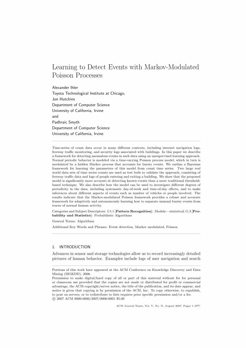
Fig. 1. Jittered scatterplot of the number of people entering on any weekday over a fifteen week

period, shown as a function of the time of day (in half-hour intervals). Although certain points(e.g., set A) clearly represent unusual periods of increased activity, it is less clear which, if any, ofthe values in set B represent something similar.

on the internet, RFID traces, security video archives, and loop-sensor records offreeway traffic. These time series often reflect the underlying hourly, daily, andweekly rhythms of natural human activity. At the same time, the time series areoften corrupted by events corresponding to bursty periods of unusual behavior. Ex-amples include anomalous bursts of activity on a network, large occasional meetingsin a building, traffic accidents, and so forth.

In this paper we address the problem of identifying such events, by learning thepatterns of both normal behavior and events from historical data. While at firstglance this problem might seem relatively straightforward, the problem becomesdifficult in an unsupervised context when events are not labeled or tagged in thedata. Learning a model of normal behavior requires the removal of the abnormalevents from the historical record—but detecting the abnormal events can be ac-complished reliably only by knowing the baseline of normal behavior. This leadsto a “chicken and egg” problem that is the main focus of this paper.

We focus in particular on time series data where time is discrete and N(t) is ameasurement of the number of individuals or objects engaged in some activity overthe time-interval [t−1, t], e.g., counts of the number of people who enter a buildingevery 15 minutes, or the number of vehicles that pass a certain location on thefreeway every 5 minutes. As an example, Figure 1 shows counts of the estimatednumber of people entering a building over time from an optical sensor at the frontdoor of a UC Irvine (UCI) campus building. The data are “jittered” slightly byGaussian noise to give a better sense of the density of counts at each time. Thereare parts of this signal which are clearly periodic, and other parts which are obviousoutliers; but there are many samples which fall into a gray area. For example, set(A) in Figure 1 is clearly far from the typical behavior for their time period; butset (B) contains many points which are somewhat unusual but may or may notbe due to the presence of an event. In order to separate the two, we need todefine a model of uncertainty (how unusual is the measurement?), and additionallyincorporate a notion of event persistence, i.e., the idea that a single, somewhatunusual measurement may not signify anything but several in a row could indicatethe presence of an event.

ACM Journal Name, Vol. V, No. N, August 2007.

· 3

6:00 12:00 18:00

20

40

Time

Veh

icle

Cou

nt

6:00 12:00 18:00

20

40

Time

Veh

icle

Cou

nt

(a) (b)

Fig. 2. Example of freeway traffic data for Fridays for a particular on-ramp. (a) Average timeprofile for normal, non game-day Fridays (dark curve) and data for a particular Friday (6/10/05)with a baseball game that night (light curve). (b) Average time profile over all Fridays (darkcurve) superposed on the same Friday data (light curve) as in the top panel.

Another example of this chicken-and-egg problem is illustrated in Figure 2. Thetop panel shows vehicle counts every five minutes for an on-ramp on the 101 freewayin Los Angeles (LA) located near Dodger Stadium, where the LA Dodgers baseballteam plays their home games. The darker line shows the average count for theset of “normal” Fridays when there were no baseball games (averaged over everynon game-day Friday for each specific 5-minute time slice). The daily rhythm ofnormal Friday vehicle flow is clear from the data: little traffic in the early hours ofthe morning, followed by a sharp consistent increase during the morning rush hour,relatively high volume and variability of traffic during the day, another increase forthe evening rush hour, and a slow decay into the night back to light traffic.

The light line in the top panel shows the counts for a particular Friday whenthere was a baseball game: the “event” can be seen in the form of significantlyincreased traffic around 22:00 hours, corresponding to a surge of vehicles leavingfrom the baseball stadium. It is clear that relative to the average profile (the darkerline) that the baseball traffic is anomalous and should be relatively easy to detect.

Now consider what would happen if we did not know when the baseball gameswere being held. The lower panel shows the time series for the same Friday as thetop panel (the lighter line) but now with the average over all Fridays superposed,i.e., the average time-profile including both game-day and non game-day Fridays.This average profile has now been pulled upwards around 22:00 hours and sitsroughly halfway between normal traffic for that time of night (the darker line inthe top panel) and the profile that corresponds to a baseball event (the light curve).Ideally we would like to learn both the patterns of normal behavior and to detectevents that indicate departures from the norm. For example, given the time seriesshown in Figure 2, we would like to learn a model that reflects the bimodal natureof such data, namely a combination of the normal traffic patterns and occasionaladditional counts caused by aperiodic events.

2. RELATED WORK AND OUTLINE OF THE PAPER

There has been a significant amount of prior work in both data mining and statisticson finding surprising patterns, outliers, and change-points in time series. For ex-ample, Keogh et al. [2002] described a technique that represents a real-valued timeseries by quantizing into it a finite set of symbols and then used a Markov model todetect surprising patterns in the symbol sequence. Guralnik and Srivastava [1999]


4 ·

proposed an iterative likelihood-based method for segmenting a time series intopiecewise homogeneous regions. Salmenkivi and Mannila [2005] investigated theproblem of segmenting sets of low-level time-stamped events into time-periods ofrelatively constant intensity, using a combination of Poisson models and Bayesianestimation methods. Kleinberg [2002] demonstrated how a method based on aninfinite automaton could be used to detect bursty events in text streams.

All of these approaches share a common goal with that of this paper, namelydetection of novel and unusual data points or segments in time series. However,none of this earlier work focuses on the specific problem we address here, namelydetection of bursty events embedded in time series of counts that reflect the normaldiurnal and calendar patterns of human activity.

The framework we propose to address this problem is derived from the Markov–modulated Poisson processes used by Scott and Smyth [2003] for analysis of Websurfing behavior and Scott [2002] for telephone network fraud detection. We extendthis work by employing a more flexible model of event-related counts as well as al-lowing for missing data. We adopt a Bayesian approach to learning and inference,allowing us to pose and answer a variety of queries within a probabilistic frame-work, such as “did any events occur in this time-period?”, “how many additionalcounts were caused by a particular event?”, “what is the estimated duration of anevent?”, and so forth. Different high-level questions about the data can also beaddressed, such as “are Monday and Tuesday normal patterns the same?” or “arethe patterns of normal behavior consistent over time or changing?” using Bayesianmodel selection techniques.

The remainder of the paper proceeds by first describing, in Section 3, the two datasets used throughout the paper: freeway traffic data and entry/exit counts for abuilding. Section 4 illustrates the limitations of a simple baseline approach to eventdetection based on thresholding. In Section 5 we describe our proposed probabilisticmodel and Section 6 describes how this model can be learned from data using aBayesian estimation framework. Section 7 discusses how we can use the learnedmodel for event detection and validates the model’s predictions of anomalous eventsusing known ground-truth schedules of events. We show that our proposed approachis significantly more accurate in practice than a baseline threshold-based method.Section 8 describes how the model can be used to answer other, related inferencequestions, such as investigating different degrees of time-heterogeneity in the modeland estimating event attendance. In Section 9 we conclude with a brief discussionof open research problems and summary comments.

3. DATA SET CHARACTERISTICS

We use two different data sets throughout the paper to illustrate our approach. Inthis section we describe these data sets in more detail.

The first data set will be referred to as the building data, consisting of fifteenweeks of count data automatically recorded every 30 minutes at the front door ofthe Calit2 institute building on the UC Irvine campus. The data are generated by apair of battery–powered optical detectors that measure the presence and directionof objects as they pass through the building’s main set of doors. The number ofcounts in each direction are then communicated via a wireless link to a base station


· 5

(a)

S M T W T F S S M T W T F S S M T W T F S

20

40

Time

Doo

r C

ount

N+(t)

(b)


20

40

Time

Doo

r C

ount

N−(t)

Fig. 3. (a) Entry data for the main entrance of the Calit2 building for three weeks,beginning 7/23/05 (Sunday) and ending 8/13/05 (Saturday). (b) Exit data for thesame door over the same time period.

with internet access, where they are stored.

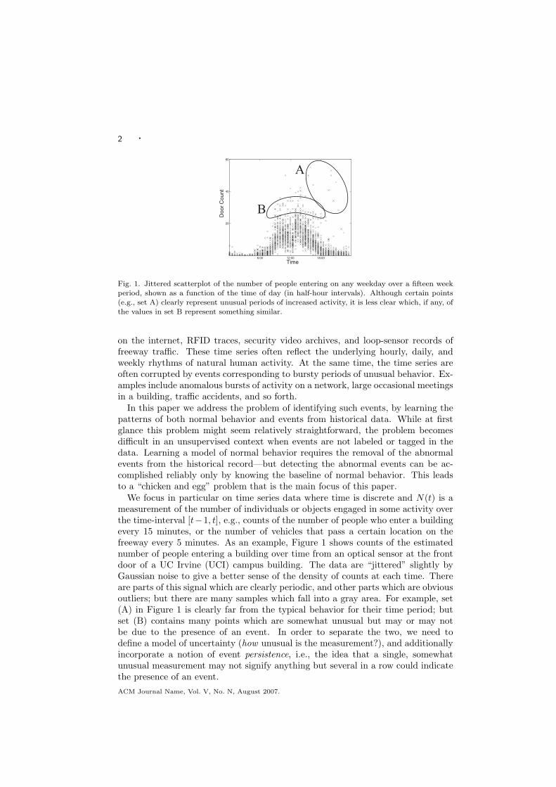
The observation sequences (“door counts”) acquired at the front door form anoisy time series with obvious structure but many outliers (see Figure 3). The dataare corrupted by the presence of events, namely, non-periodic activities which takeplace in the building and (typically) cause an increase in foot traffic entering thebuilding before the event, and leaving the building after the event, possibly withadditional people going in and out during the event. Some of these events can beseen easily in the time–series, for example the two large spikes in both entry andexit data on days four and twelve in Figure 3. However, many of these events maybe less obvious and only become visible when compared to the behavior over a longperiod of time.

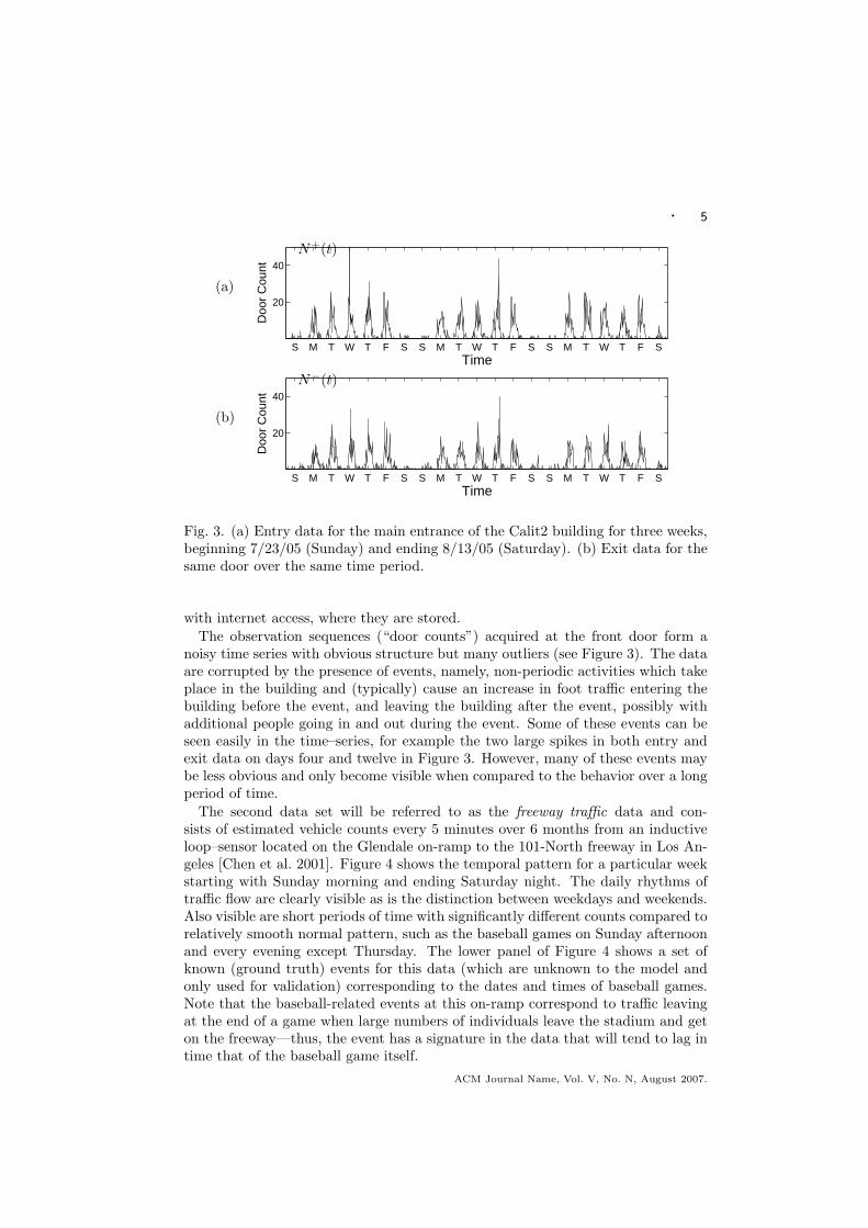
The second data set will be referred to as the freeway traffic data and con-sists of estimated vehicle counts every 5 minutes over 6 months from an inductiveloop–sensor located on the Glendale on-ramp to the 101-North freeway in Los An-geles [Chen et al. 2001]. Figure 4 shows the temporal pattern for a particular weekstarting with Sunday morning and ending Saturday night. The daily rhythms oftraffic flow are clearly visible as is the distinction between weekdays and weekends.Also visible are short periods of time with significantly different counts compared torelatively smooth normal pattern, such as the baseball games on Sunday afternoonand every evening except Thursday. The lower panel of Figure 4 shows a set ofknown (ground truth) events for this data (which are unknown to the model andonly used for validation) corresponding to the dates and times of baseball games.Note that the baseball-related events at this on-ramp correspond to traffic leavingat the end of a game when large numbers of individuals leave the stadium and geton the freeway—thus, the event has a signature in the data that will tend to lag intime that of the baseball game itself.


6 ·

SUN MON TUE WED THU FRI SAT

20

40

Veh

icle

Cou

nt

eventsTime

(a)

(b)

Fig. 4. (a) One week of traffic data (light curve) from Sunday to Saturday (June 5-11), with the

estimated normal traffic profile (estimated by the proposed model described later in the paper)superposed as a dark curve. (b) Ground truth list of events (baseball games).

4. SIMPLE POISSON MODELS

Let N(t), for t ∈ {1, . . . , T}, generically refer to the observed count at time t forany of the time-dependent counting processes, such as the freeway traffic 5-minuteaggregate count process or either of the two (entering or exiting) building 30-minuteaggregate door count processes.

Perhaps the most common probabilistic model for count data is the Poissondistribution, whose probability mass function is given by

P(N ;λ) = e−λλN/N ! N = 0, 1, . . . (1)

where the parameter λ represents the rate, or average number of occurrences ina fixed time interval. When λ is a function of time, i.e. λ(t), (1) becomes anonhomogeneous Poisson distribution, in which the degree of heterogeneity dependson the function λ(t).

4.1 Testing the Poisson Assumption

The assumption of a Poisson distribution may not always hold in practice, and it isreasonable to ask whether it fits the data at hand. For a simple Poisson distributionthere are a number of classical goodness-of-fit tests which can be applied, such asthe chi-squared test [Papoulis 1991]. However, in this case we typically have a largenumber of potentially different rates, each of which has only a few observationsassociated with it. For example in the freeway traffic data, there are 2016 five-minute time slices in a week, each of which may be described by a different rate,and for each time-slice there are between 22 and 25 non-missing observations overthe 25 weeks of our study.

Although classical extensions for hypothesis testing exist in such situations [Svens-son 1981], here we use a more qualitative approach since our goal is simply to assesswhether the Poisson assumption is reasonable for the data. Specifically, we knowthat, if the data are Poisson, the true mean and variance of the observations ateach time slice should be equal. Given finite data, the empirical mean and varianceat each time provide noisy estimates of the true mean and variance, and we canvisually assess whether these estimates are close to equal by comparing them to the


· 7

10 20 30 40

100

200

300

Mean

Var

ianc

e

10 20 30 40

20

40

60

80

MeanV

aria

nce

0 5 10 15 20 25

20

40

60

Mean

Var

ianc

e

(a) (b) (c)

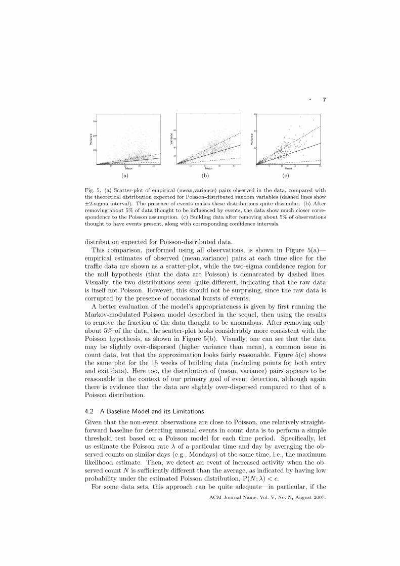
Fig. 5. (a) Scatter-plot of empirical (mean,variance) pairs observed in the data, compared withthe theoretical distribution expected for Poisson-distributed random variables (dashed lines show

±2-sigma interval). The presence of events makes these distributions quite dissimilar. (b) Afterremoving about 5% of data thought to be influenced by events, the data show much closer corre-spondence to the Poisson assumption. (c) Building data after removing about 5% of observationsthought to have events present, along with corresponding confidence intervals.

distribution expected for Poisson-distributed data.This comparison, performed using all observations, is shown in Figure 5(a)—

empirical estimates of observed (mean,variance) pairs at each time slice for thetraffic data are shown as a scatter-plot, while the two-sigma confidence region forthe null hypothesis (that the data are Poisson) is demarcated by dashed lines.Visually, the two distributions seem quite different, indicating that the raw datais itself not Poisson. However, this should not be surprising, since the raw data iscorrupted by the presence of occasional bursts of events.

A better evaluation of the model’s appropriateness is given by first running theMarkov-modulated Poisson model described in the sequel, then using the resultsto remove the fraction of the data thought to be anomalous. After removing onlyabout 5% of the data, the scatter-plot looks considerably more consistent with thePoisson hypothesis, as shown in Figure 5(b). Visually, one can see that the datamay be slightly over-dispersed (higher variance than mean), a common issue incount data, but that the approximation looks fairly reasonable. Figure 5(c) showsthe same plot for the 15 weeks of building data (including points for both entryand exit data). Here too, the distribution of (mean, variance) pairs appears to bereasonable in the context of our primary goal of event detection, although againthere is evidence that the data are slightly over-dispersed compared to that of aPoisson distribution.

4.2 A Baseline Model and its Limitations

Given that the non-event observations are close to Poisson, one relatively straight-forward baseline for detecting unusual events in count data is to perform a simplethreshold test based on a Poisson model for each time period. Specifically, letus estimate the Poisson rate λ of a particular time and day by averaging the ob-served counts on similar days (e.g., Mondays) at the same time, i.e., the maximumlikelihood estimate. Then, we detect an event of increased activity when the ob-served count N is sufficiently different than the average, as indicated by having lowprobability under the estimated Poisson distribution, P(N ;λ) < ǫ.

For some data sets, this approach can be quite adequate—in particular, if the


8 ·

May 17 May 18

20

40

0

1

Time

May 17 May 18

20

40

0

1

Time

[ L ] [ R ]

(a)

(b)

(c)

Veh

icle

count

p(z 6= 0)

events

Fig. 6. [L]: Illustration of the baseline threshold model set to detect the event on the second day,with (a) original freeway traffic time series (light curve) for May 17-18, and mean profile as usedby the threshold model (dark curve), (b) events detected by the threshold method, and (c) ground

truth (known events) in the bottom panel. Note the false alarms. [R]: Using a lower threshold todetect the full duration of the large event on the second day, causing many more false alarms.

events interspersed in the data are sufficiently few compared to the amount of non–event observations, and if they are sufficiently noticeable in the sense that theycause a dramatic change in activity. However, these assumptions do not alwayshold, and we can observe several modes of failure in such a simple model.

One way this model can fail is due to the “chicken and egg” problem mentionedin the introduction and illustrated in Figure 2. As discussed earlier, the presenceof large events distorts the estimated rate of “normal”behavior, which causes thethreshold test to miss the presence of other events around that same time.

A second type of failure occurs when there is a slight change in traffic levelwhich is not of sufficient magnitude to be noticed; however, the change is sustained

over a period of several observations signaling the presence of a persistent event. InFigure 6[L], the event indicated for the first day can be easily found by the thresholdmodel by setting the threshold sufficiently high enough to detect the event but lowenough so that there are no false alarms. In order for the threshold model to detectthe event on the second day, however, the threshold must be decreased, which alsocauses the detection of a few false alarms over the two-day period. Anomaliesdetected by the threshold model are shown in Figure 6[L](b), while the knownevents (baseball games) are displayed in panel (c).

A third weakness of the threshold model is its difficulty in capturing the durationof an event. In order to detect not only the presence of the event on the second daybut also its duration, the threshold must be raised to the point that the numberof false alarms becomes quite prohibitive, as illustrated in Figure 6[R]. Note thatthe traffic event, corresponding to people departing the game, begins at or near theend of the actual game time.

In the remaining sections of the paper we discuss a more sophisticated proba-bilistic model that accounts for these different aspects of the problem, and show(in Section 7) that it can be used to obtain significantly more accurate detectionperformance than the simple thresholding method.


· 9

5. PROBABILISTIC MODELING

Section 4, and in particular the failures of Figure 6, motivate the use of a probabilis-tic model capable of reasoning simultaneously about the rate of normal behavior(intuitively corresponding to the periodic portion of the data) and the presence andduration of events (relatively rare deviations from the norm). Let us assume thatthe two processes are additive, so that

N(t) = N0(t) + NE(t), N(t) ≥ 0 (2)

where N0(t) is the number of occurrences attributed to the normal building oc-cupancy, and NE(t) represents the change in the number of occurrences which isattributed to an event at time t (positive or negative); the non-negativity conditionindicates that we cannot observe fewer than zero counts. We discuss modeling eachof the variables N0, NE in turn. Note that, although the models described hereare defined for discrete time periods, it may also be possible to extend them tocontinuous time measurements [Scott 1998; 2002].

5.1 Modeling Periodic Count Data

To model the periodic, predictable portion of behavior corresponding to normalactivity, we use a nonhomogeneous Poisson process (see Section 4) with a particularparameterization of the rate λ(t); our model is derived from that of Scott [1998],and has been used to detect and segment fraud patterns in telephone networkusage [Scott 2002]. Specifically, we decompose λ(t) as

λ(t) = λ0 δd(t) ηd(t),h(t) (3)

where d(t) takes on values {1, . . . , 7} and indicates the day on which time t falls (sothat Sunday = 1, Monday = 2, and so forth), and h(t) indicates the interval (e.g.,half-hour periods for the building data) in which time t falls. By further requiring

that∑7

j=1 δj = 7 and∑D

i=1 ηj,i = D ∀j, where D is the number of time intervalsin a day (48 for the building data and 288 for the freeway traffic data), we canensure that the values λ0, δ, and η are easily interpretable: λ0 is the average rateof the Poisson process over a full week, δj is the day effect, or the relative changefor day j (so that, for example, Sundays have a lower rate than Mondays), and ηj,i

is the relative change in time period i given day j (the time of day effect).Figure 7 illustrates these two effects for the building data. Figure 7(a) shows

one week’s worth of data alongside the estimated rate with day effect only, i.e.,λ0 δd(t); this is the full Poisson rate λ(t) averaged over the time of day. Figure 7(b)then shows how ηd(t),h(t) then modulates λ(t) over a single day to achieve a sensibletime–dependent rate value.

Graphical models provide a useful and general formalism for characterizing thedependence structure among a set of random variables [Jordan 1998]. In a directedgraphical model or Bayesian network, directed edges indicate a factorization of thejoint distribution into a product of conditionals, in which each node depends onlyon the values of its parents in the graph. Figure 8(a) shows a graphical model inthe form of a plate diagram for the periodic data N0(t) and associated parameters.The plate notation (shown as a rectangle in Figure 8(a)) is used in graphical modelsto indicate sets of replicated variables that are conditionally independent given


10 ·

SUN MON TUE WED THU FRI SAT

5

10

15

20

Time

Doo

r C

ount

Counts

Mean

Day

6:00 12:00 18:00

5

10

15

20

Time

Doo

r C

ount

Counts

Mean

Day

ToD Effect

(a) (b)

Fig. 7. (a) The effect of δd(t), as seen over a week of building exit data. The relative rates over theweekend (Sunday, Saturday) are much lower than those on weekdays. (b) The effect of ηd(t),h(t)

in modulating the Poisson rate of building exit data over a single day. There is a noticeable peakaround lunchtime, and a heavy bias towards the end of the day.

common parent nodes that are outside the plate [Buntine 1994]. The plates indicatethat there are multiple variables λ(t) and N0(t), one for each value of t ∈ {1 . . . T},and that the λ(t) variables are conditionally independent of each other given λ0,σ, and η. A key point is that, given N0(t), the parameters λ0, δ, and η are allindependent of N(t).

By choosing conjugate prior distributions for these variables we can ensure thatthe inference computations in Section 6 have a simple closed form:

λ0 ∼ Γ(λ; aL, bL)

1

7[δ1, . . . , δ7] ∼ Dir(αd

1, . . . , αd7)

1

D[ηj,1, . . . , ηj,D] ∼ Dir(αh

1 , . . . , αhD)

where Γ is the Gamma distribution,

Γ(λ; a, b) ∝ λa−1e−bλ

and Dir(·) is a Dirichlet distribution with the specified parameter vector.

5.2 Modeling Rare, Persistent Events

In the data examined in this paper, the anomalous measurements can be intuitivelythought of as being due to relatively short, rare periods in which an additional ran-dom process changes the observed behavior, increasing or decreasing the number ofobserved counts. In cases of increased activity (“positive” events), these deviationsmay arise from the presence of some cause (e.g., people arriving for an event in thebuilding), while decreased activity patterns (“negative” events) can be thought ofas a suppression or removal of counts which would normally have been observed.

To model the behavior of anomalous periods of time, we use a ternary processz(t) to indicate the presence of an event and its type, i.e.,

z(t) =

0 if there is no event at time t

+1 if there is a positive event

−1 if there is a negative event


· 11

λ0

δ

η

λ(t)

N0(t)

1 : T z(t − 1) z(t) z(t + 1)

N0(t)NE(t)

N(t)

(a) (b)

Fig. 8. (a) Graphical model for λ(t) and N0(t). The parameters λ0, δ, and η (the periodiccomponents of λ(t)) couple the distributions over time. (b) Graphical model for z(t) and N(t).

The Markov structure of z(t) couples the variables over time [in addition to the coupling of N0(t)from (a)].

and define the probability distribution over z(t) to be Markov in time, with tran-sition probability matrix

Mz =

z00 z0+ z0−

z+0 z++ z+−

z−0 z−+ z−−

with each row summing to one, e.g., z00 + z0+ + z0− = 1. These variables canbe interpreted in terms of intuitive characteristics of the system; for example, thelength of each time period between events is geometric with expected value 1/(1−z00), the length of each positive event is geometric with expected value 1/(1−z++),and so forth. We give the transition probability variables priors specified as

[z00, z0+, z0−] ∼ Dir(z ; [aZ00, aZ

0+, aZ0−])

and similarly for the other matrix rows, where Dir(·) is again the Dirichlet distri-bution.

Given z(t), we can model the increase or decrease in observation counts due tothe event, NE(t), as Poisson with rate γ(t)

NE(t) ∼

{

0 z(t) = 0

P( z(t)N ; γ(t)) z(t) 6= 0

and γ(t) as independent at each time t

γ(t) ∼ Γ(γ; aE , bE).

In fact, γ(t) may be marginalized over analytically, since∫

P(N ; γ)Γ(γ; aE , bE) = NBin(N ; aE , bE/(1 + bE)) (4)

where NBin is the negative binomial distribution. A graphical model representingthe distribution over z(t), NE(t), and N(t) is shown in Figure 8(b). Here, z(t)provides the time–dependent structure of the process; from Figure 8(a)–(b), onecan see that N(t) has temporal structure both from λ(t) and z(t).


12 ·

This type of gated Poisson contribution, called a Markov–modulated Poissonmodel, is a common component of many network traffic models [Heffes and Lucan-toni 1984; Scott 2002]. In our application we are specifically interested in detectingthe periods of time in which the event process z(t) is active, and we can use the rateγ(t) or the associated count NE(t) to provide information about its “popularity.”While it is also possible to couple the rates γ(t) in order to capture the idea that,for example, two detections at times t and t + 1 are likely to be related and thushave correlated count increases, we do not address this additional complexity here.

6. LEARNING AND INFERENCE

Let us initially assume that our total length of observation comprises some integralnumber of weeks, so that T = 7 ∗D ∗W for some integer W . Although not strictlynecessary, this assumption greatly simplifies the inference procedure for estimatingthe parameters of the model [Scott 2002]. In fact it is not restrictive in our setting,since we can always extend a region of interest to cover an integer number of weeksby taking the additional data to be unobserved.

Given the complete data {N0(t), NE(t), z(t)}, it is straightforward to computemaximum a posteriori (MAP) estimates or draw posterior samples of the parametersλ(t) and Mz, since all variables λ0, δ, η, and Mz are conditionally independent (seeFigure 8 or Section 6.2).

We can thus infer posterior distributions over each of the variables of interestusing Markov chain Monte Carlo (MCMC) methods [Geman and Geman 1984;Gelfand and Smith 1990]. Specifically, we iterate between drawing samples of thehidden variables {z(t), N0(t), NE(t)} (described in Section 6.1) and the parametersgiven the complete data (described in Section 6.2). The complexity of each iterationof MCMC is O(T ), linear in the length of the time series. Experimentally we havefound that the sampler converges quite rapidly on the data sets used in this paper,where convergence is informally assessed by monitoring the parameter values andvalues of the marginal likelihood. For both data sets used in this paper, 10 burn-initerations followed by 50 more sampling iterations appeared quite sufficient. Inpractice, on a 3GHz Xeon desktop machine in Matlab, the building data (15 weeksof 30-minute intervals) took about 3 minutes while the traffic data (25 weeks of5-minute intervals) took about one hour. The samples obtained from MCMC canbe used to not only to provide a point estimate of the value of each parameter(for example, its posterior mean) but also to gauge the amount of uncertaintyabout that value. If this degree of uncertainty is not of interest (for example, ifthe data are sufficiently many that the uncertainty is very small) we could use analternative method such as expectation–maximization (EM) to learn the parametervalues [Buntine 1994].

6.1 Sampling the Hidden Variables Given Parameters

Given the periodic Poisson mean λ(t) and the transition probability matrix M ,it is relatively straightforward to draw a sample sequence z(t) using a variant ofthe forward–backward algorithm [Baum et al. 1970]. We provide below the nec-essary equations for completeness. Specifically, in the forward pass we compute,for each t ∈ {1, . . . , T} the conditional distribution p(z(t)|{N(t′), t′ ≤ t}) using the


· 13


10

20

Doo

r C

ount

0

0.5

1

Time

N+(t)

(a)

(b) p(z 6= 0)

(c) events:

Fig. 9. (a) Entry data, along with λ(t), over a period of three weeks (Sept. 25–Oct. 15). Also shown are (b) the posterior probability of an event being present,p(z(t) 6= 0), and (c) the periods of time in which an event was scheduled for thebuilding. All but one of the scheduled events are detected, along with a few othertime periods (such as a period of greatly heightened activity on the first Saturday).

likelihood functions

p(N(t)|z(t)) =

P(N(t);λ(t)) z(t) = 0∑

i P(N(t) − i;λ(t))NBin(i) z(t) = +1∑

i P(N(t) + i;λ(t))NBin(i) z(t) = −1

(where the parameters of NBin(·) are as in (4)). Then, for t ∈ {T, . . . , 1}, we drawsamples

Z(t) ∼ p( z(t) | z(t + 1) = Z(t + 1), {N(t′), t′ ≤ t} ).

Given z(t) = Z(t), we can then determine N0(t) and NE(t) by sampling. If z(t) =0, we simply take N0(t) = N(t); if z(t) = +1 we draw N0(t) from the discretedistribution

N0(t) ∼ f+(i) ∝ P(N(t) − i;λ(t))NBin(i; aE , bE/(1 + bE))

and if z(t) = −1 from the distribution

N0(t) ∼ f−(i) ∝ P(N(t) + i;λ(t))NBin(i; aE , bE/(1 + bE))

then setting NE(t) = N(t) − N0(t). Note that, if z(t) = +1, N0 takes values in{0 . . . N}; if z(t) = −1, however, N0 has no fixed upper limit. In practice, forcomputational efficiency we truncate the distribution (imposing an upper limit) atthe point given by P(N(t) + i;λ(t)) < 10−4.

When N(t) is unobserved (missing), N0(t) and NE(t) are coupled only throughz(t) and the positivity condition on N(t). Thus, when z(t) 6= −1 (positive or noevent), N0 and NE can be drawn independently, and when z(t) = −1 (negativeevent) they can be drawn fairly easily through rejection sampling, i.e., repeat-edly drawing the variables independently until they satisfy the positivity condition.Overall, missing data are relatively rare, with essentially no observations missing


14 ·

in the building data and about 7% of observations missing in the traffic data (dueto loop sensor errors or down-time).

6.2 Sampling the Parameters Given the Complete Data

Because T is an integral number of weeks, T = 7 ∗ D ∗ W , the complete datalikelihood is

∏

t

e−λ(t)λ(t)N0(t)∏

t

p(Z(t)|Z(t − 1))∏

Z(t)=1

NBin(NE(t))

Considering the first term, which only involves λ0, δ, and η, we have

e−Tλ0λP

N0(t)0

∏

j

δP

d(t)=jN0(t)

j

∏

j,i

η(...)j,i

By virtue of choosing conjugate prior distributions, the posteriors are distributionsof the same form, but with parameters given by the sufficient statistics of the data.Defining

Sj,i =∑

t:d(t)=j,

h(t)=i

N0(t) Sj =∑

i

Sj,i S =∑

j

Sj

the posterior distributions are

λ0 ∼ Γ(λ; aL + S, bL + T )

1

7[δ1, . . . , δ7] ∼ Dir(αd

1 + S1, . . . , αd7 + S7)

1

D[ηj,1, . . . , ηj,D] ∼ Dir(αh

1 + Sj,1, . . . , αhD + Sj,D).

Sampling the transition matrix parameters {z00, z0+, . . . z−−} is similarly straightforward—we compute

Zij =∑

t:z(t)=i,z(t+1)=j

1 for i, j ∈ {0,+1,−1}

to obtain the posterior distribution

[z00, z0+, z0−] ∼ Dir(z; [aZ00 + Z00, aZ

0+ + Z0+, aZ0− + Z0−])

and similar forms for the other zij . As noted by Scott [2002], Markov–modulatedPoisson processes appear to be relatively sensitive to the selection of prior distri-butions over the zij and γ(t), perhaps because there are no direct observations ofthe processes they describe. This appears to be particularly true for our model,which has considerably more freedom in the anomaly process (i.e., in γ(t)) than thetelephony application of Scott [2002]. However, for an event detection applicationsuch as those under consideration, we have fairly strong ideas of what constitutesa “rare” event, e.g., approximately how often we expect to see events occur (say,1–2 per day) and how long we expect them to last (perhaps an hour or two).We can leverage this information to form relatively strong priors on the transitionparameters of z(t) which force the marginal probability of z(t). This avoids over-explanation of the data, such as using the event process to compensate for the fact


· 15

that the “normal” data exhibits slightly larger than expected variance for Poissondata (see Section 4.1). By adjusting these priors one can also increase or decreasethe model’s sensitivity to deviations and thus the number of events detected; seeSection 7.

7. ADAPTIVE EVENT DETECTION

One of the primary goals in our application is to automatically detect the presenceof unusual events in the observation sequence. The presence or absence of theseevents is captured by the process z(t), and thus we may use the posterior probabilityp(z(t) 6= 0|{N(t)}) as an indicator of when such events occur.

Given a sequence of data, we can use the samples drawn in the MCMC proce-dure (Section 6) to estimate the posterior marginal distribution over events. Forcomparison to a ground truth of the events in the building data set, we obtaineda list of the events which had been scheduled over the entire time period from thebuilding’s event coordinator. For the freeway traffic data set, the game times for78 home games in the LA Dodgers 2005 regular season were used as the validationset. Three additional regular season games were not included in this set becausethey occurred during extended periods of missing loop sensor count information.Note that both sets of “ground truth” may represent an underestimate of the truenumber of events that occurred (e.g., due to unscheduled meetings and gatherings,concerts held at the baseball stadium, etc.). Nonetheless this ground truth is veryuseful in terms of measuring how well a model can detect a known set of events.

The results obtained by performing MCMC for the building data are shown inFigure 9. We plot the observations N(t) together with the posterior mean of therate parameters λ(t) over a three week period (Sept. 25–Oct. 15); Figure 9 showsincoming (entry) data for the building. Displayed below the time series is theposterior probability of z(t) 6= 0 at each time t, drawn as a sequence of bars, belowwhich dashes indicate the times at which scheduled events in the building tookplace. In this sequence, all of the known events are successfully detected, alongwith a few additional detections that were not listed in the building schedule. Suchunscheduled activities often occur over weekends where the baseline level of activityis particularly low.

Figure 10 shows a detailed view of one particular day, during which there wasan event scheduled in the building atrium. Plots of the probability of an unusualevent for both the entering and exiting data show a high probability over the entireperiod allocated to the event, while slight increases earlier in the day were deemedmuch less significant due to their relatively short duration.

The results obtained by performing MCMC for the freeway traffic data for threegame-days are shown in Figures 11–12. Figure 11 shows a Friday game that ismore sparsely attended than the Friday game plotted in Figure 2 and providesan example in which our model successfully separates the normal Friday eveningactivity from game-day evening activity. The threshold model was able to detectthe Friday games with heavy attendance, but more sparsely attended games suchas this one were missed.

Figure 12 displays the same two–day period as Figure 6, where the thresholdmodel was shown to detect false alarms when the threshold level was set low enough


16 ·

10

20

0

0.5

1

6:00 12:00 18:00Time

10

20

0

0.5

1

6:00 12:00 18:00Time

p(z 6= 0)

N+(t) N−(t)

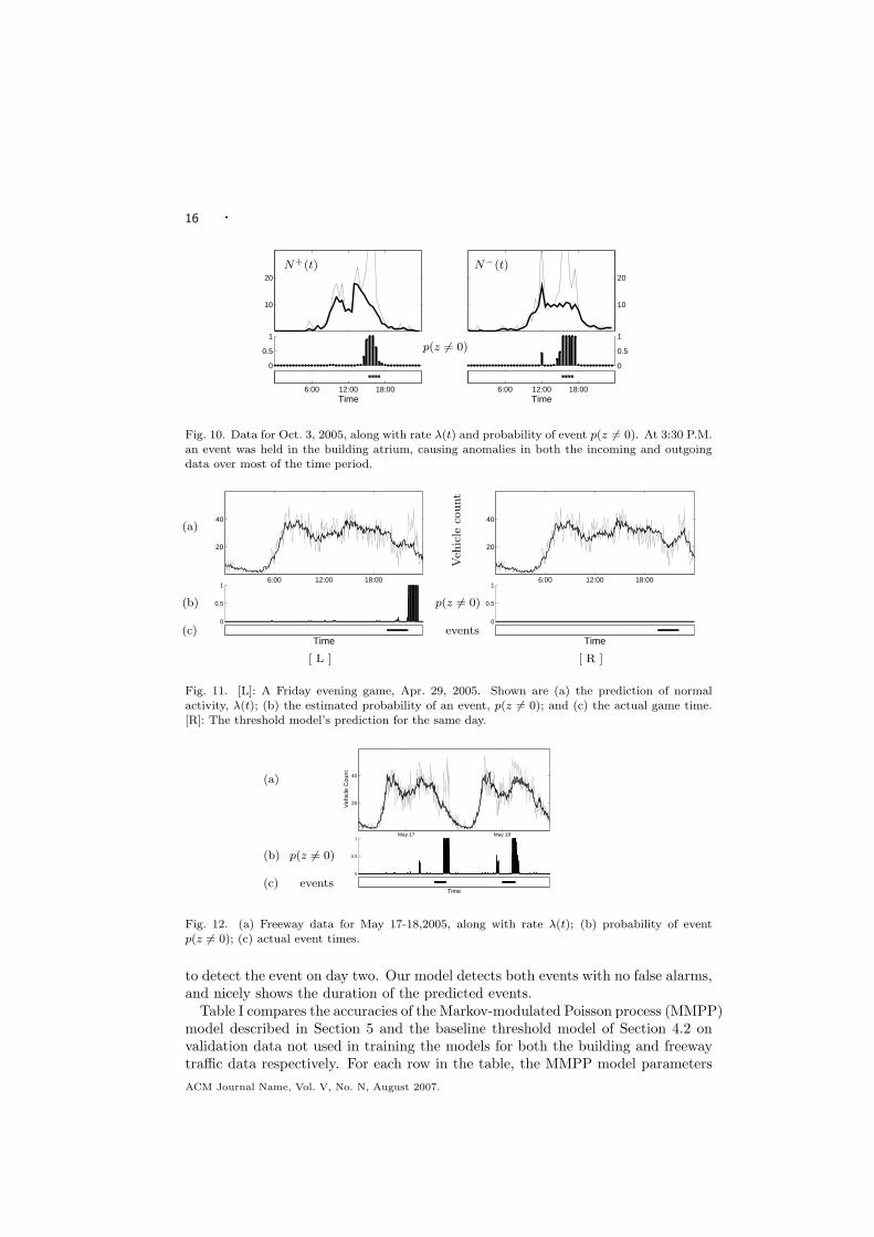
Fig. 10. Data for Oct. 3, 2005, along with rate λ(t) and probability of event p(z 6= 0). At 3:30 P.M.an event was held in the building atrium, causing anomalies in both the incoming and outgoing

data over most of the time period.

6:00 12:00 18:00

20

40

0

0.5

1

Time

6:00 12:00 18:00

20

40

0

0.5

1

Time

[ L ] [ R ]

(a)

(b)

(c)

Veh

icle

count

p(z 6= 0)

events

Fig. 11. [L]: A Friday evening game, Apr. 29, 2005. Shown are (a) the prediction of normal

activity, λ(t); (b) the estimated probability of an event, p(z 6= 0); and (c) the actual game time.[R]: The threshold model’s prediction for the same day.

May 17 May 18

20

40

Veh

icle

Cou

nt

0

0.5

1

Time

(a)

(b)

(c)

p(z 6= 0)

events

Fig. 12. (a) Freeway data for May 17-18,2005, along with rate λ(t); (b) probability of eventp(z 6= 0); (c) actual event times.

to detect the event on day two. Our model detects both events with no false alarms,and nicely shows the duration of the predicted events.

Table I compares the accuracies of the Markov-modulated Poisson process (MMPP)model described in Section 5 and the baseline threshold model of Section 4.2 onvalidation data not used in training the models for both the building and freewaytraffic data respectively. For each row in the table, the MMPP model parameters


· 17

Building Data: Freeway Data:

Total # of MMPP ThresholdPredicted Events Model Model

149 100.0% 89.7%98 86.2% 82.8%

68 79.3% 65.5%

Total # of MMPP ThresholdPredicted Events Model Model

355 100.0% 85.9%264 100.0% 82.1%

154 100.0% 66.7%

129 97.4% 55.1%

Table I. Accuracies of predictions for the two data sets, in terms of the percentages of knownevents found by each model, for different total numbers of events predicted. There were 29 knownevents in the building data, and 78 in the freeway data.

were adjusted so that a specific number of events were detected, by adjusting thepriors on the transition probability matrix. The threshold model was then modifiedto find the same number of events as the MMPP model by adjusting its thresholdǫ.

In both data sets, for a fixed number of predicted events (each row), the numberof true events detected by the MMPP model is significantly higher than that ofthe baseline model. This validates the intuitive discussion of Section 4.2 in whichwe outlined some of the possible limitations of the baseline approach, namely itsinability to solve the “chicken and egg” problem and the fact that it does notexplicitly represent event persistence. As mentioned earlier, the events detected bythe MMPP model that are not in the ground truth list may plausibly correspond toreal events rather than false alarms, such as unscheduled activities for the buildingdata and accidents and non-sporting events for the freeway traffic data.

Negative events (corresponding to lower than expected activity) tend to be morerare than positive events (higher than expected activity), but can play an importantrole in the model. For example, in the building data the presence of holidays(during which very little activity is observed) can corrupt the estimates of normalbehavior. If known, these days can be explicitly removed (marked as missing) [Ihleret al. 2006], but by treating such periods as negative events the model can be maderobust to such periods. Although negative events are quite rare in the building data(comprising about 5% of the events detected), they are more common in the trafficdata set (about 40% of events). Figure 13 shows a typical example of a negativetraffic event. Here, only three cars were observed on the ramp during a 15 minuteperiod with normally high traffic followed by a 30 minute period with much higherthan normal activity. We might speculate that the initial negative event could bedue to an accident or construction, which shut down the ramp for a short period,followed by a positive event during which the resulting build-up of cars were finallyallowed onto the highway.

8. OTHER INFERENCES

Given that our model is capable of detecting and separating the influence of unusualperiods of activity, we may also wish to use the model to estimate other quantitiesof interest. For example, we can separate out the normal patterns of behavior anduse a goodness-of-fit test to answer questions about the degree of heterogeneity inthe data and thus the underlying human behavior. Alternatively, we might wishto use our estimates of the amounts of abnormal behavior to infer other, indirectly


18 ·

6:00 12:00 18:00

20

40

Veh

icle

Cou

nt

0

0.5

1p(z=−1)

0

0.5

1p(z=+1)

Time

(a)

(b)

(c)

Fig. 13. Negative and positive events: (a) Freeway data and estimated profile for May 6; (b) when

the number of observed cars drops sharply, the probability of a negative event is high; (c) thedecrease is followed by a short but large increase in traffic, detected as a positive event.

related aspects of the event, such as its popularity or importance. We discuss eachof these cases next.

8.1 Testing Heterogeneity

One question we may wish to ask about the data is, how time–varying is the processitself? For example, how different is Friday afternoon from that of any other week-day? By increasing the number of degrees of freedom in our model, we improve itspotential for accuracy but may increase the amount of data required to learn themodel well. This also has important consequences in terms of data representation(for example, compression), which may need to be a time–dependent function aswell. Thus, we may wish to consider testing whether the data we have acquiredthus far supports a particular degree of heterogeneity.

We can phrase many of these questions as tests over sub-models which requireequality among certain subsets of the variables. For example, we may wish to testfor the presence of the day effect, and determine whether a separate effect for eachday is warranted. Specifically, we might test between three possibilities:

D0 : δ1 = . . . = δ7 (all days the same)

D1 : δ1 = δ7, δ2 = . . . = δ6 (weekends, weekdays the same)

D2 : δ1 6= . . . 6= δ7 (all day effects separate)

We can compare these various models by estimating each of their marginal like-lihoods [Gelfand and Dey 1990]. The marginal likelihood is the likelihood of thedata under the model, having integrated out the uncertainty over the parametervalues, e.g.,

p(N |D2) =

∫

p(N |λ0, δ, η)p(λ0, δ, η) ∂λ0 ∂δ ∂η

Since uncertainty over the parameter values is explicitly accounted for, there is noneed to penalize for an increasing number of parameters. Moreover, we can use thesame posterior samples drawn during the MCMC process (Section 6) to find themarginal likelihood, using the estimate of Chib [1995].

Computing the marginal likelihoods for each of the models D1, . . . ,D3 for thebuilding data, and normalizing by the number of observations T , we obtain thevalues shown in Table II. From these values, it appears that D0 (all days the same)


· 19

Model E[log2 p(N−(t))] E[log2 p(N+(t))]

D0 -2.86 -2.58D1 -2.55 -2.29D2 -2.55 -2.29

Table II. Average log marginal likelihood of the data (exit and entry) under various day–

dependency models: D0, all days the same; D1, weekends and weekdays separate; and D2, eachday separate. There does not appear to be a significant change in behavior among weekend daysor among weekdays. Parameters ηi,j were unconstrained.

Model E[log2 p(N−(t))] E[log2 p(N+(t))]

T0 -2.58 -2.30T1 -2.52 -2.27T2 -2.55 -2.29

Table III. Average log marginal likelihood under various time-of-day dependency models for thebuilding data: T0, all days have the same time profile; T1, weekend days and weekdays share timeprofiles; T2, each day has its own individual time profile. The model appears to slightly prefer T1,

indicating strong profile similarities among weekdays and among weekends. Parameters δj wereunconstrained.

is a considerably worse model, and that D1 and D2 are essentially equal, indicatingthat either model will do an equally good job of predicting behavior.

We can derive similar tests for other symmetries that might exist. For example,we might wonder whether every day has the same time profile. (Note that this ispossible, since Sunday might be a severely squashed version of Monday, i.e., fewerpeople come to work, but they follow a similar hourly pattern.) Alternatively,is each day of the week unique, or (again) might all weekdays be the same, andsimilarly weekend days? Our tests become

T0 : ∀i, η1,i = . . . = η7,i (same time every day)

T1 : ∀i, η1,i = η7,i, η2,i = . . . = η6,i (weekends, weekdays)

T2 : ∀i, η1,i 6= . . . 6= η7,i (all time effects separate)

The results, shown in Table III, show a small but distinct preference for T1, indi-cating that although weekends and weekdays have differing profiles, one can betterpredict behavior by combining data across weekdays and weekends. Other tests,such as whether Fridays differ from other days, can be accomplished using similarestimates.

8.2 Estimating Event Attendance

Along with estimating the probability that an unusual event is taking place, as partof the inference procedure our model also estimates the number of counts whichappear to be associated with that event. Marginalizing over the other variables,we obtain a distribution over how many additional (or fewer) people seem to beentering or leaving the building or the number of extra (or missing) vehicles enteringthe freeway during a particular time period. One intriguing use for this informationis to provide a score, or some measure of popularity, of each event.

As an example, taking our collection of LA Dodgers baseball games, we compute


20 ·

0 100 200 300 400 500 6003

4

5

6x 10

4

number of extra vehicles

gam

e at

tend

ance

Fig. 14. The attendance of each baseball game (y-axis) shows correlation with the number ofadditional (event–related) vehicles detected by the model (x-axis).

and sum the posterior mean of extra (event-related) vehicles observed, NE(t), dur-ing the duration of the event detection. Figure 14 shows that our estimate of thenumber of additional cars is positively correlated with the actual overall attendancerecorded for the games (correlation coefficient 0.67). Similar attendance scores canbe computed for the building data, or other quantities such as duration estimated,though for these examples no ground truth exists for comparison.

9. CONCLUSION

We have described a framework for building a probabilistic model of time–varyingcounting processes, in which we observe a superposition of both time–varying butregular (periodic) and aperiodic processes. We then applied this model to twodifferent time series of counts of the number of people entering and exiting throughthe main doors of a campus building and the number of vehicles entering a freeway,both over several months. We described how the parameters of the model maybe estimated using MCMC sampling methods, while simultaneously detecting thepresence of anomalous increases or decreases in the counts. This detection processnaturally accumulates information over time, and by virtue of having a modelof uncertainty provides a natural way to compare potentially anomalous eventsoccurring on different days or times.

Using a probabilistic model also allows us to pose alternative models and testamong them in a principled way. Doing so we can answer questions about how theobserved behavior varies over time, and how predictable that behavior is. Finally,we described how the information obtained in the inference process can be used toprovide an interesting source of feedback, for example estimating event popularityand attendance.

Although the current model is very effective in accurately detecting events in thedata sets we looked at, it is also a relatively simple model and there are a numberof potential extensions that could improve its performance for specific applications.For example, the Poisson parameters for nearby time-periods could be coupled inthe model to share information during learning and encourage smoothness in theinferred mean profiles over time. Similarly, it could be valuable to incorporateadditional exogenous variables into the proposed model, e.g., allowing both normaland event-based intensities to be dependent on factors such as weather. The eventprocess could be generalized from a Markov to a semi-Markov process to handleevents with specific (non-geometric) duration signatures. In principle all of theseextensions could be handled via appropriate extensions of the graphical models


· 21

and Bayesian estimation techniques described earlier in the paper, with attendantincreases in modeling and computational complexity.

A further interesting direction for future work is to simultaneously model multiplecorrelated time series, such as those arising from door counts from multiple doors(and perhaps from more than one type of sensor) as well as multiple time seriesfrom different loop sensors along a freeway. More sensors provide richer informationabout occupancy and behavioral patterns, but it is an open question how these co-varying data streams should be combined, and to what degree their parameters canbe shared.

Acknowledgments

The authors would like to thank Chris Davison and Anton Popov for their as-sistance with logistics and data collection, and Shellie Nazarenus for providing alist of scheduled events for the Calit2 building. This material is based upon worksupported in part by the National Science Foundation under Award Numbers ITR-0331707, IIS-0431085, and IIS-0083489.

REFERENCES

Baum, L. E., Petrie, T., Soules, G., and Weiss, N. 1970. A maximization technique occurringin statistical analysis of probabilistic functions of Markov chains. Annals of Mathematical

Statistics 41, 1 (February), 164–171.

Buntine, W. 1994. Operations for learning with graphical models. Journal of Artificial Intelli-

gence Research 2, 159–225.

Chen, C., Petty, K., Skabardonis, A., Varaiya, P., and Jia, Z. 2001. Freeway performancemeasurement system: mining loop detector data. 80th Annual Meeting of the TransportationResearch Board, Washington, D.C. http://pems.eecs.berkeley.edu/.

Chib, S. 1995. Marginal likelihood from the Gibbs output. Journal of the American Statistical

Association 90, 432 (Dec.), 1313–1321.

Gelfand, A. E. and Dey, D. K. 1990. Bayesian model choice: asymptotics and exact calculations.Journal of Royal Statistical Society, Series C 56, 3, 501–514.

Gelfand, A. E. and Smith, A. F. M. 1990. Sampling-based approaches to calculating marginal

densities. Journal of the American Statistical Association 85, 398–409.

Geman, S. and Geman, D. 1984. Stochastic relaxation, Gibbs distributions, and the Bayesian

restoration of images. IEEE Transactions on Pattern Analysis and Machine Intelligence 6, 6(Nov.), 721–741.

Guralnik, V. and Srivastava, J. 1999. Event detection from time series data. In KDD ’99:

Proceedings of the fifth ACM SIGKDD international conference on Knowledge discovery and

data mining. ACM Press, New York, NY, USA, 33–42.

Heffes, H. and Lucantoni, D. M. 1984. A Markov-modulated characterization of packetizedvoice and data traffic and related statistical multiplexer performance. IEEE Journal on Selected

Areas in Communications 4, 6, 856–868.

Ihler, A., Hutchins, J., and Smyth, P. 2006. Adaptive event detection with time–varying Pois-son processes. In KDD ’06: Proceedings of the twelfth ACM SIGKDD international conference

on Knowledge discovery and data mining. ACM Press, New York, NY, USA, 207–216.

Jordan, M. I., Ed. 1998. Learning in Graphical Models. MIT Press, Cambridge, MA.

Keogh, E., Lonardi, S., and chi’ Chiu, B. Y. 2002. Finding surprising patterns in a time series

database in linear time and space. In KDD ’02: Proceedings of the eighth ACM SIGKDD

international conference on Knowledge discovery and data mining. ACM Press, New York,NY, USA, 550–556.


22 ·

Kleinberg, J. 2002. Bursty and hierarchical structure in streams. In KDD ’02: Proceedings of

the eighth ACM SIGKDD international conference on Knowledge discovery and data mining.ACM Press, New York, NY, USA, 91–101.

Papoulis, A. 1991. Probability, Random Variables, and Stochastic Processes, 3rd ed. McGraw-Hill Inc., New York, NY.

Salmenkivi, M. and Mannila, H. 2005. Using Markov chain Monte Carlo and dynamic pro-gramming for event sequence data. Knowledge and Information Systems 7, 3, 267–288.

Scott, S. 1998. Bayesian methods and extensions for the two state Markov modulated Poissonprocess. Ph.D. thesis, Harvard University, Dept. of Statistics.

Scott, S. 2002. Detecting network intrusion using a Markov modulated nonhomogeneous Poissonprocess. http://www-rcf.usc.edu/∼sls/mmnhpp.ps.gz.

Scott, S. L. and Smyth, P. 2003. The Markov modulated Poisson process and Markov Poissoncascade with applications to web traffic data. Bayesian Statistics 7, 671–680.

Svensson, A. 1981. On a goodness of fit test for multiplicative Poisson models. The Annals of

Statistics 9, 4, 697–704.


learning to detect events with markov-modulated poisson ... · learning to detect events with...

Documents