Learning to Integrate Web Taxonomies

Dell Zhang1,2

1Department of Computer Science School of Computing

S15-05-24, 3 Science Drive 2 National University of Singapore

Singapore 117543 2Singapore-MIT Alliance

E4-04-10, 4 Engineering Drive 3 Singapore 117576 Tel: +65-68744251 Fax: +65-67794580

dell.z@ieee.org

Wee Sun Lee1,2 1Department of Computer Science

School of Computing SOC1-05-26, 3 Science Drive 2 National University of Singapore

Singapore 117543 2Singapore-MIT Alliance

E4-04-10, 4 Engineering Drive 3 Singapore 117576 Tel: +65-68744526 Fax: +65-67794580

leews@comp.nus.edu.sg

ABSTRACT We investigate machine learning methods for automatically integrating objects from different taxonomies into a master taxonomy. This problem is not only currently pervasive on the Web, but is also important to the emerging Semantic Web. A straightforward approach to automating this process would be to build classifiers through machine learning and then use these classifiers to classify objects from the source taxonomies into categories of the master taxonomy. However, conventional machine learning algorithms totally ignore the availability of the source taxonomies. In fact, source and master taxonomies often have common categories under different names or other more complex semantic overlaps. We introduce two techniques that exploit the semantic overlap between the source and master taxonomies to build better classifiers for the master taxonomy. The first technique, Cluster Shrinkage, biases the learning algorithm against splitting source categories by making objects in the same category appear more similar to each other. The second technique, Co-Bootstrapping, tries to facilitate the exploitation of inter-taxonomy relationships by providing category indicator functions as additional features for the objects. Our experiments with real-world Web data show that these proposed add-on techniques can enhance various machine learning algorithms to achieve substantial improvements in performance for taxonomy integration.

Keywords Semantic Web, Ontology Mapping, Taxonomy Integration, Classification, Machine Learning.

1. INTRODUCTION A taxonomy, or directory or catalog, is a division of a set of objects (documents, images, products, goods, services, etc.) into a set of categories. There are a tremendous number of taxonomies on the Web, and we often need to integrate objects from various taxonomies into a master taxonomy.

This problem is currently pervasive on the Web, given that many websites are aggregators of information from various other websites [1]. For example, a Web marketplace like Amazon1 may want to combine goods from multiple vendors’ catalogs into its own; a Web portal like NCSTRL2 may want to combine documents from multiple libraries’ directories into its own; a company may want to merge its service taxonomy with its partners’; a researcher may want to merge his/her bookmark taxonomy with his/her peers’; Singapore-MIT Alliance 3, an innovative engineering education and research collaboration among MIT, NUS and NTU, has a need to integrate the academic resource (course, seminar, report, software, etc.) taxonomies of these three universities.

This problem is also important to the emerging Semantic Web [2], where data has structures and ontologies describe the semantics of the data, thus better enabling computers and people to work in cooperation. On the Semantic Web, data often come from many different ontologies, and information processing across ontologies is not possible without knowing the semantic mappings between them. Since taxonomies are central components of ontologies, ontology mapping necessarily involves finding the correspondences between two taxonomies, which is often based on integrating objects from one taxonomy into the other and vice versa [3, 4].

If all taxonomy creators and users agreed on a universal standard, taxonomy integration would not be so difficult. But the Web has evolved without central editorship. Hence the correspondences between two taxonomies are inevitably noisy and fuzzy. For illustration, consider the taxonomies of two Web portals Google4 and Yahoo5: what is “Arts/ Music/Styles/” in one may be “Entertainment/Music/Genres/” in the other, category “Computers_and_Internet/ Software/Freeware/” and category “Computers/Open_Source/Software/” have similar contents but show non-trivial differences, and so on. It is unclear if a universal standard will appear outside specific domains, and even for those domains, there is a need to integrate objects from legacy taxonomies into the standard taxonomy.

Manual taxonomy integration is tedious, error-prone, and clearly not possible at the Web scale. A straightforward approach to automating this process would be to formulate it as a classification problem, a problem that has been well-studied in the machine learning area [5]. Conventional machine learning algorithms would simply train classifiers on the master taxonomy data while totally ignoring the source taxonomy data. However, the availability of the source taxonomy data could be helpful to build better classifiers for the master taxonomy if there is some

1 http://www.amazon.com/ 2 http://www.ncstrl.org/ 3 http://web.mit.edu/sma/ 4 http://www.google.com/ 5 http://www.yahoo.com/

semantic overlap between the source and master taxonomies, particularly when the number of training examples is not very large.

One of the simplest assumptions that can be helpful for improving learning is that each source category is likely to be mapped entirely into a master category. Under this assumption, it is helpful to bias the learning algorithm to prefer functions that do not split objects of the source categories into different master categories. Agrawal and Srikant proposed the Enhanced Naive Bayes algorithm [1] which modifies the Naive Bayes algorithm [5] such that if most of the objects from a source category are classified into a single master category, it intends to classify more objects from that source category into that master category. This has the effect of reducing the number of objects that are classified differently from the majority class within a source category. In this paper, we describe a different mechanism, Cluster Shrinkage, which biases learning algorithms that use object distance/similarity measures from splitting the objects in a source category into different master categories. This is done by changing the distance/similarity measure so that objects in the same source category become closer to each other. We applied this technique to the Transductive Support Vector Machine [6-8] and the Spectral Graph Transducer [9].

While useful, assuming that each source category is mapped entirely into a master category is clearly simplistic. Potentially useful semantic relationships between a master category C and a source category S include: • C S= (identical): an object belongs to C if and only if it belongs to S ; • C S = ∅∩ (mutual exclusion): if an object belongs to S it cannot belong to C ; • C S⊇ (superset): any object that belonging to S must also belong to C ;

• C S⊆ (subset): any object not belonging to S also cannot belong to C ;

• C and S overlap but neither is a superset of the other. In addition, semantic relationships may involve multiple source and master categories. For example, a master category C may be a subset of the union of two source categories aS and bS , so if an object does not belong to

either aS or bS , it cannot belong to C . The real-world semantic relationships are noisy and fuzzy, but they can still

provide valuable information for classification. For example, knowing that most (80%) objects in a source category S belong to one master category aC and the rest (20%) of the examples belong to another master category bC is

obviously helpful. The difficulty is that knowledge about those semantic relationships is not explicit but hidden in the data. One method of exploiting these relationships without explicitly knowing them is to include indicator variables for source categories as additional features for the objects so that machine learning algorithms can utilize such information. Unfortunately the values of these variables are not known for the objects in the master taxonomy which we use for learning. We propose an iterative technique that alternatively uses information in the source and master taxonomies to construct the required features for taxonomies. We call this technique Co-Bootstrapping as it “bootstraps” on the information from the classifier of the other taxonomy in order to improve itself at each iteration. We applied this technique to the AdaBoost algorithm [10-12] and the Support Vector Machine [13, 14].

Our experiments on the datasets from two of today's main Web taxonomies (Google/Dmoz and Yahoo) show that all the proposed techniques can enhance various machine learning algorithms to achieve substantial improvements in performance for taxonomy integration. The Co-Bootstrapping technique, which may be able to exploit more source-master relationships than the Cluster Shrinkage technique, appears to give better performance although we have not done extensive experimentation on this comparison.

The rest of this paper is organized as follows. In section 2, we give the formal problem statement. In section 3-5, we describe Enhanced Naive Bayes, Cluster Shrinkage and Co-Bootstrapping. In section 6, we conduct experimental evaluations. In section 7, we review the related work. In section 8, we discuss hierarchical taxonomies and other extensions. In section 9, we make concluding remarks.

2. PROBLEM STATEMENT Taxonomies are often organized as hierarchies. In this work, we assume for simplicity that any objects assigned to an interior node really belong to a leaf node which is an offspring of that interior node. Since we now have all objects only at leaf nodes, we can flatten the hierarchical taxonomy to a single level and treat it as a set of categories [1]. Possible extensions that may be able to exploit the presence of hierarchies are discussed in section 8.

Now we formally define the taxonomy integration problem that we are solving. Given two taxonomies: • a master taxonomy M with a set of categories 1 2, ,..., MC C C each containing a set of objects, and

• a source taxonomy N with a set of categories 1 2, ,..., NS S S each containing a set of objects,

we need to find the correct categories in M for each object in N.

The objects in M are called master objects, and the objects in N are called source objects. 1 2, ,..., MC C C are called

master categories, and 1 2, ,..., NS S S are called source categories.

To formulate taxonomy integration as a classification problem, we take master categories 1 2, ,..., MC C C as classes, the

master objects as training examples and the source objects as test examples, so that taxonomy integration can be automatically accomplished by predicting the classes of each test example. Such a classification problem has several prominent characteristics: • it is essentially a multi-class multi-label classification problem, in the sense that there could be more than two

possible classes (multi-class) and one object could belong to more than one class (multi-label); • the test examples are already known to the machine learning algorithm; • the test examples are already labeled with a set of categories which are usually not identical with but relevant to

the set of categories to be assigned.

For machine learning algorithms that only lead to binary (positive/negative) classifiers, multi-class multi-label classification could be achieved via the popular one-vs-rest ensemble method: creating a binary classifier for each class iC that takes the objects belonging to iC as positive examples and all other objects as negative examples. For

the binary classifier corresponding to iC , we denote the class of negative examples (objects that do not belong to iC )

by iC .

Some of the algorithms for this problem require a tune set, i.e., a set of objects whose source categories and master categories are all known, to find the optimal values of its parameters. To achieve good performance using those algorithms, there should be an adequate number of objects in the tune set. If the set of master objects and the set of source objects have a decent size intersection, then this intersection can act as a tune set. Otherwise, a tune set can only be made available by selecting a subset of source objects and manually labeling their master categories. Selection of the source objects to be placed in the tune set can be done via random sampling or active learning [1].

In this paper, we focus on text data, i.e., objects in taxonomies are actually documents. Other types of data can be treated using similar techniques.

3. THE ENHANCED NAIVE BAYES TECHNIQUE In this section, we describe Agrawal and Srikant’s Enhanced Naïve Bayes (ENB) algorithm [1] for taxonomy integration.

3.1 Naïve Bayes Naïve Bayes (NB) is a well-known text classification algorithm [5]. NB tries to fit a generative model for documents using training examples and then apply this model to classify test examples. The generative model of NB assumes that a document is generated by first choosing its class according to a prior distribution of classes, and then producing its words independently according to a (typically multinomial) distribution of terms conditioned on the chosen class [15].

Given a test document d , NB classifies d into a class iC if and only if Pr[ | ] Pr[ | ]i iC d C d> . The posterior

probability Pr[ | ]C d can be computed via Bayes’s rule:

Pr[ | ]C d Pr[ , ]

Pr[ ]

C d

d=

Pr[ ]Pr[ | ]

Pr[ ]

C d C

d= Pr[ ]Pr[ | ]C d C∝ .

The probability Pr[ ]C can be estimated by

Pr[ ]C

iiC

C

C=∑

,

where C is the number of training documents in C . With the “naïve” assumption that the words of d occur

independently given the class C , the probability Pr[ | ]d C can be estimated by

Pr[ | ]d C ( ) ( , )Pr[ | ]

n d w

w dw C

∈= ∏ ,

where ( , )n d w is the number of occurrences of w in d . The probability Pr[ | ]w C can be estimated by

Pr[ | ]w C ( )( , )

( , )i

iw V

n C w

n C w

ηη

∈

++

=∑

,

where ( , )n C w is the number of occurrences of w in training documents in C , V is the vocabulary of terms, and

0 1η< ≤ is the Lidstone’s smoothing parameter [16]. Taking logs, we see that NB is actually a linear classifier:

log Pr[ | ]C d ( )( )( , )log Pr[ ] Pr[ | ]

n d w

w dC w C

∈∝ ∏ ( ) log Pr[ ]( , ) log Pr[ | ]

w dCn d w w C

∈= × +∑ .

3.2 Enhanced Naïve Bayes Suppose that the classifier predicts that 90% of the objects in the source category S fall in the master category C and the other 10% fall in other master categories. Those 10% that fall in the other master categories are probably prediction errors [1]. We can exploit this idea to enhance classification performance by making the master categories that own a large percentage of objects from S receive more objects from S and at the same time making the master categories that own a small percentage of objects from S receive fewer objects from S . One effect of doing this is that it reduces the likelihood of splitting source categories, particularly those with most objects classified into one master category.

Agrawal and Srikant recently proposed the Enhanced Naïve Bayes (ENB) algorithm [1] according to the above idea. They assumed that one document only belongs to one master category. Here we relax this assumption and extend their ENB algorithm to multi-class multi-label classification via the one-vs-rest method (as stated in section 2).

Given a source document d in a source category S , ENB classifies it into a master category iC if and only if

Pr[ | , ] Pr[ | , ]i iC d S C d S> . The posterior probability Pr[ | , ]C d S can be computed as

Pr[ | , ]C d S Pr[ , , ]

Pr[ , ]

C d S

d S=

Pr[ ]Pr[ , | ]

Pr[ , ]

S C d S

d S= Pr[ , | ]C d S∝ .

ENB invokes a simplification that assumes d and S are independent given C , therefore

Pr[ , | ]C d S Pr[ | ]Pr[ | , ]C S d S C= Pr[ | ]Pr[ | ]C S d C= ( ) ( , )Pr[ | ] Pr[ | ]

n d w

w dC S w C

∈= ∏ .

The probability Pr[ | ]w C can be estimated in the same way as in NB.

For the probability Pr[ | ]C S , a simple estimation could be achieved by first using trained NB classifiers to tentatively classify source objects (test examples) into master categories (classes). and then calculating

Pr[ | ]C S C S

S

←=

C

C S

C S

←

←=∑

,

where S is the number of documents in S and C S← is the number of documents in S that are classified into

C by NB. However, this simple estimation is based on NB’s classification result and is therefore not so reliable. As

an illustration, consider a scenario where we know that the categorizations of M and N are exactly identical. With a

perfect classifier, the above estimation should be 1 for the true class and 0 for all other classes. With a classifier that is 90% accurate, the above estimation would be 0.9 for the true class and 0.1 distributed over all other classes. In this case, we would like to increase Pr[ | ]C S for the class having most examples from S and decrease Pr[ | ]C S for all

other classes. More generally, we would like to use a parameter 0ω ≥ that reflects the degree of semantic overlap

between M and N to decide the strength of such induction bias. In addition, we would like to use Pr[ ]C to smooth

the estimation of Pr[ | ]C S . ENB uses an estimation formula that satisfies theses goals:

Pr[ | ]C S ( )C

C C S

C C S

ω

ω

× ←

× ←=∑

C C Sω∝ × ← .

Taking logs, we see that ENB is still a linear classifier:

log Pr[ | , ]C d S ( )( )( , )log Pr[ | ] Pr[ | ]

n d w

w dC S w C

∈∝ ∏ ( )( , ) log Pr[ | ] logPr[ | ]n d w w C C Sw d= × +∑ ∈ .

When a source document d belongs to multiple source categories (1) (2) ( ), ,..., gS S S , the above ENB formulas should

be amended by substituting (1) (2) ( ), ,..., gS S S for S .

Comparing the classification functions of ENB and NB, it is obvious that all ENB does is to shift the classification thresholds of its base NB classifiers, no more and no less. When 0ω = , ENB is same as NB. When 0ω > , we have the following result from [1] which indicates that ENB tends to re-classify the documents from S into the classes with more S-documents.

THEOREM 1 [1]. Let xC S← denote the number of documents in S that are classified into xC by NB. For any

document d in a source category S , suppose ENB with parameter 1 0ω ≥ predicts its class to be 1x

C and ENB with

parameter 2 0ω ≥ predicts its class to be 2xC . If 1 2ω ω> , then

1 2x xC S C S← ←≥ .

From the above theorem, we see that a document d in a source category S can only switch from a class with fewer S-documents to a class with more S-documents and not the other way around as ENB increases its parameter ω . This

has the effect of reducing the number of objects that are classified differently from the majority class within a source category. A good value for ω can be found using a tune set.

4. THE CLUSTER SHRINKAGE TECHNIQUE In this section, we describe the Cluster Shrinkage technique in detail, and show how it can enhance the Transductive Support Vector Machine [6-8] and the Spectral Graph Transducer [9] for taxonomy integration.

4.1 Vector Space Model Documents (text objects) can be represented as vectors using Vector Space Model [17]. For each document d in a collection of documents D , it is first pre-processed by removal of stop-words and stemming, and then represented as a feature vector 1 2( , , ..., )mx x x=x , where ix indicates the importance weight of term iw (the i-th distinct word

occurred in D ). Following the popular TF×IDF weighting scheme, we set the value of ix to the product of the term

frequency ( , )iTF w d and the inverse document frequency ( )iIDF w , i.e., ( , ) ( )i iTF w d IDF w× . The term frequency

( , )iTF w d means the number of occurrences of iw in d . The inverse document frequency is defined as

( )( ) log ( )i iIDF w D DF w= , where D is the total number of documents in D , and ( )iDF w is the number of

documents in which iw occur. Finally all feature vectors are normalized to have unit length.

4.2 Support Vector Machine Support Vector Machine (SVM) [13, 14] is a powerful machine learning algorithm which has shown outstanding classification performance in practice. It is based on a solid theoretical foundation — structural risk minimization [18].

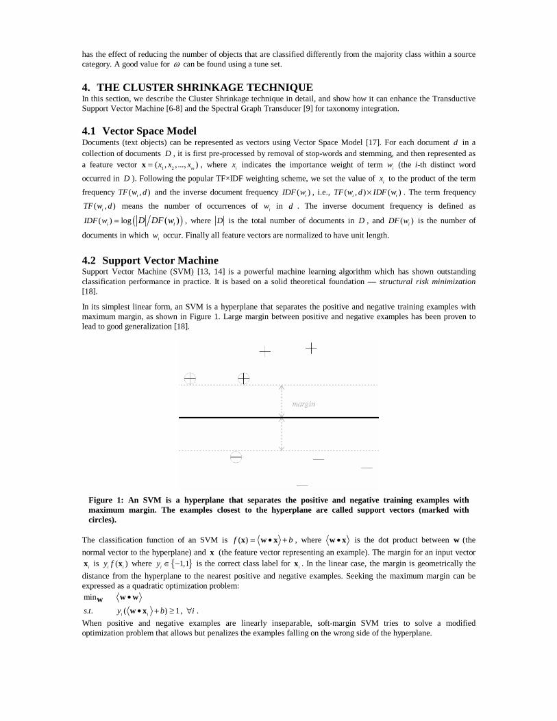
In its simplest linear form, an SVM is a hyperplane that separates the positive and negative training examples with maximum margin, as shown in Figure 1. Large margin between positive and negative examples has been proven to lead to good generalization [18].

The classification function of an SVM is ( )f b= • +x w x , where •w x is the dot product between w (the

normal vector to the hyperplane) and x (the feature vector representing an example). The margin for an input vector

ix is ( )i iy f x where { }1,1iy ∈ − is the correct class label for ix . In the linear case, the margin is geometrically the

distance from the hyperplane to the nearest positive and negative examples. Seeking the maximum margin can be expressed as a quadratic optimization problem: minw •w w

. .s t ( ) 1i iy b• + ≥w x , i∀ .

When positive and negative examples are linearly inseparable, soft-margin SVM tries to solve a modified optimization problem that allows but penalizes the examples falling on the wrong side of the hyperplane.

Figure 1: An SVM is a hyperplane that separates the positive and negative training examples with maximum margin. The examples closest to the hyperplane are called support vectors (marked with circles).

4.3 Transductive Learning Regular learning algorithms try to induce a general classification function which has high accuracy on the whole distribution of examples. However, this so-called inductive learning setting is often unnecessarily complex. For the classification problem in taxonomy integration context, the set of test examples to be classified are already known to the learning algorithm. In fact, we do not care about the general classification function, but rather attempt to achieve good classification performance on that particular set of test examples. This is exactly the goal of transductive learning [6].

The transductive learning task is defined on a fixed array of n examples 1 2( , ,..., )nX = x x x . Each example has a

desired classification 1 2( , ,..., )nY y y y= , where { }1, 1iy ∈ + − for binary classification. Given the labels for a subset

[1.. ]lY n⊂ of lY l n= < (training) examples, a transductive learning algorithm attempts to predict the labels of the

remaining (test) examples in X as accurately as possible.

Why can transductive learning algorithms outperform inductive learning algorithms? Transductive learning algorithms can observe the examples in the test set and potentially exploit structure in their distribution. For example, there usually exists a clustering structure of examples: the examples in same class tend to be close to each other in feature space, and such kind of knowledge is helpful to learning, especially when there are only a small number of training examples [8].

Most machine learning algorithms assume that both the training and test examples come from the identical data distribution. This assumption does not necessarily hold in the case of taxonomy integration. Intuitively, transductive learning algorithms seem to be more robust than inductive learning algorithms to the violation of this assumption, since transductive learning algorithms takes the test examples into account for learning. This interesting issue needs to be stressed in the future.

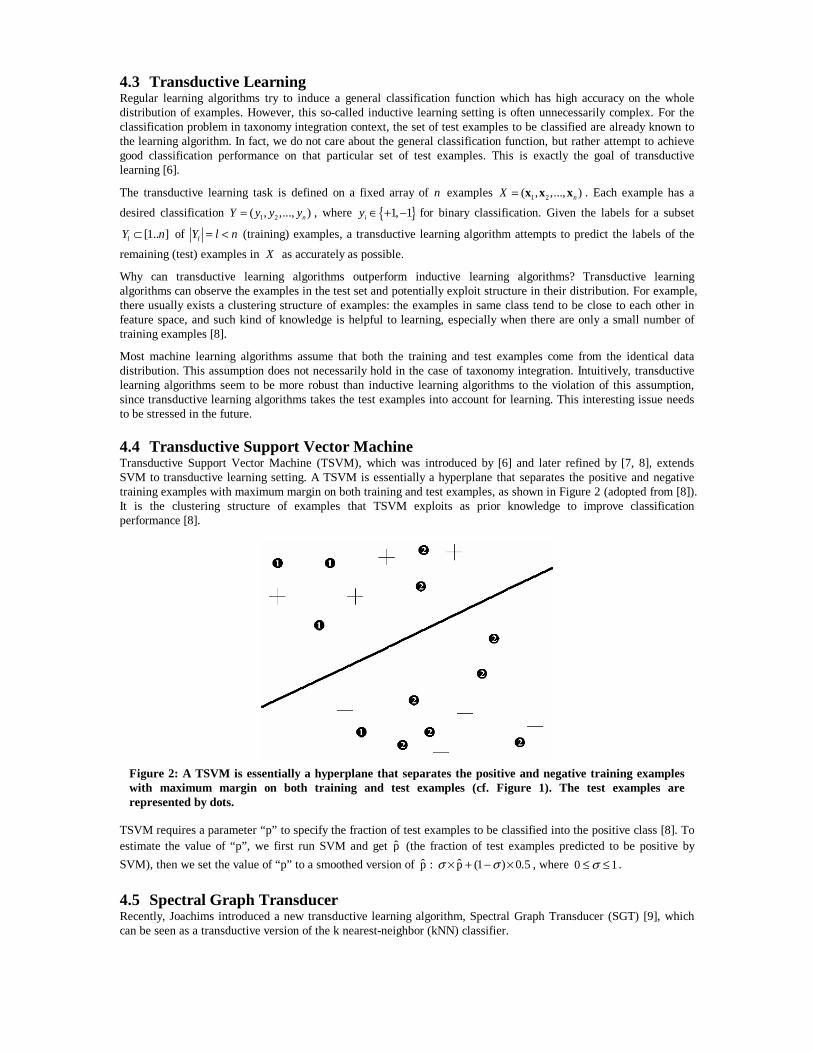
4.4 Transductive Support Vector Machine Transductive Support Vector Machine (TSVM), which was introduced by [6] and later refined by [7, 8], extends SVM to transductive learning setting. A TSVM is essentially a hyperplane that separates the positive and negative training examples with maximum margin on both training and test examples, as shown in Figure 2 (adopted from [8]). It is the clustering structure of examples that TSVM exploits as prior knowledge to improve classification performance [8].

TSVM requires a parameter “p” to specify the fraction of test examples to be classified into the positive class [8]. To estimate the value of “p”, we first run SVM and get p̂ (the fraction of test examples predicted to be positive by

SVM), then we set the value of “p” to a smoothed version of p̂ : p̂ (1 ) 0.5σ σ× + − × , where 0 1σ≤ ≤ .

4.5 Spectral Graph Transducer Recently, Joachims introduced a new transductive learning algorithm, Spectral Graph Transducer (SGT) [9], which can be seen as a transductive version of the k nearest-neighbor (kNN) classifier.

Figure 2: A TSVM is essentially a hyperplane that separates the positive and negative training examples with maximum margin on both training and test examples (cf. Figure 1). The test examples are represented by dots.

SGT works in three steps. The first step is to build the k nearest-neighbor (kNN) graph G on the set of examples X .

The kNN graph G is similarity-weighted and symmetrized: its adjacency matrix is defined as TA A A′ ′= + , where

( )

( , ) if ( )

( , )

0 elsek i

i jj i

i kij knn

simknn

simA ∈

⎧∈⎪′ = ⎨

⎪⎩

∑ x x

x xx x

x x .

The function ( , )sim ⋅ ⋅ can be any reasonable similarity measure. In the following, we will use a common similarity function

( , ) cosi j

i j

i j

sim θ•

= =x x

x xx x

,

where θ represents the angle between ix and jx . The second step is to decompose G into spectrum, specifically,

compute the smallest 2 to 1d + eigenvalues and corresponding eigenvectors of G ’s normalized Laplacian 1( )L B B A−= − , where B is the diagonal degree matrix with ii ijj

B A=∑ . The third step is to classify the examples.

Given a set of training labels lY , SGT makes predictions by solving the following optimization problem which

minimizes the normalized graph cut with constraints:

miny { } { }( , )

: 1 : 1i i

cut G G

i y i y

+ −

= + = −

. .s t 1, if and positivei ly i Y= + ∈

1, if and negativei ly i Y= − ∈

{ }1, 1n= + −y ,

where G+ and G− denote the set of examples (vertices) with 1iy = + and 1iy = − respectively, and the cut-value

( , )cut G G+ − iji G j GA+ −∈ ∈

=∑ ∑ is the sum of the edge weights across the cut (bi-partitioning) defined by G+ and

G− . Although this optimization problem is known to be NP-hard, there are highly efficient techniques based on the spectrum of the graph that give good approximation to the global optimal solution [9].

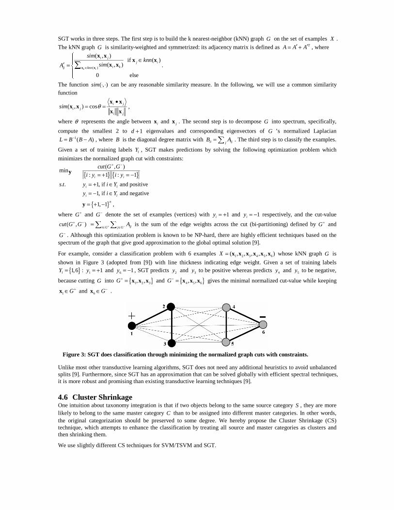
For example, consider a classification problem with 6 examples 1 2 3 4 5 6( , , , , , )X = x x x x x x whose kNN graph G is

shown in Figure 3 (adopted from [9]) with line thickness indicating edge weight. Given a set of training labels

{ }1,6lY = : 1 1y = + and 6 1y = − , SGT predicts 2y and 3y to be positive whereas predicts 4y and 5y to be negative,

because cutting G into { }1 2 3, ,G+ = x x x and { }4 5 6, ,G− = x x x gives the minimal normalized cut-value while keeping

1 G+∈x and 6 G−∈x .

Unlike most other transductive learning algorithms, SGT does not need any additional heuristics to avoid unbalanced splits [9]. Furthermore, since SGT has an approximation that can be solved globally with efficient spectral techniques, it is more robust and promising than existing transductive learning techniques [9].

4.6 Cluster Shrinkage One intuition about taxonomy integration is that if two objects belong to the same source category S , they are more likely to belong to the same master category C than to be assigned into different master categories. In other words, the original categorization should be preserved to some degree. We hereby propose the Cluster Shrinkage (CS) technique, which attempts to enhance the classification by treating all source and master categories as clusters and then shrinking them.

We use slightly different CS techniques for SVM/TSVM and SGT.

Figure 3: SGT does classification through minimizing the normalized graph cuts with constraints.

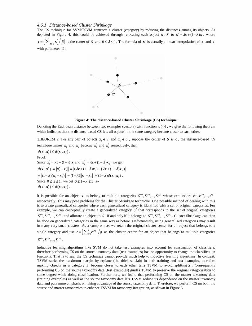
4.6.1 Distance-based Cluster Shrinkage The CS technique for SVM/TSVM contracts a cluster (category) by reducing the distances among its objects. As depicted in Figure 4, this could be achieved through relocating each object S∈x to ' (1 )λ λ= + −x c x , where

( )SS

∈= ∑x

c x is the center of S and 0 1λ≤ ≤ . The formula of ′x is actually a linear interpolation of x and c

with parameter λ .

Denoting the Euclidean distance between two examples (vectors) with function ( , )d ⋅ ⋅ , we give the following theorem which indicates that the distance-based CS lets all objects in the same category become closer to each other.

THEOREM 2. For any pair of objects 1 S∈x and 2 S∈x , suppose the center of S is c , the distance-based CS

technique makes 1x and 2x become 1′x and 2

′x respectively, then

1 2 1 2( , ) ( , )d d′ ′ ≤x x x x .

Proof: Since 1 1(1 )λ λ′ = + −x c x and 2 2(1 )λ λ′ = + −x c x , we get

1 2( , )d ′ ′x x 1 2′ ′= −x x ( ) ( )1 2(1 ) (1 )λ λ λ λ= + − − + −c x c x

1 2(1 )( )λ= − −x x 1 2(1 )λ= − −x x 1 2(1 ) ( , )dλ= − x x .

Since 0 1λ≤ ≤ , we get 0 1 1λ≤ − ≤ , so

1 2 1 2( , ) ( , )d d′ ′ ≤x x x x .

It is possible for an object x to belong to multiple categories (1) (2) ( ), ,..., gS S S whose centers are (1) (2) ( ), ,..., gc c c respectively. This may pose problems for the Cluster Shrinkage technique. One possible method of dealing with this is to create generalized categories where each generalized category is identified with a set of original categories. For example, we can conceptually create a generalized category S ′ that corresponds to the set of original categories

(1) (2) ( ), ,..., gS S S , and allocate an object to S ′ if and only if it belongs to (1) (2) ( ), ,..., gS S S . Cluster Shrinkage can then be done on generalized categories in the same way as before. Unfortunately, using generalized categories may result in many very small clusters. As a compromise, we retain the original cluster center for an object that belongs to a

single category and use ( )( )

1

g h

hg

== ∑c c as the cluster center for an object that belongs to multiple categories

(1) (2) ( ), ,..., gS S S .

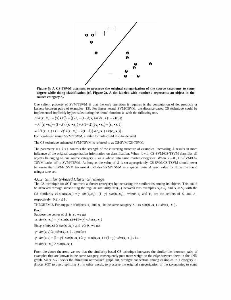
Inductive learning algorithms like SVM do not take test examples into account for construction of classifiers, therefore performing CS on the source taxonomy data (test examples) has no opportunity to change the classification functions. That is to say, the CS technique cannot provide much help to inductive learning algorithms. In contrast, TSVM seeks the maximum margin hyperplane (the thickest slab) in both training and test examples, therefore making objects in a category S become closer to each other tells TSVM to avoid splitting S . Consequently performing CS on the source taxonomy data (test examples) guides TSVM to preserve the original categorization to some degree while doing classification. Furthermore, we found that performing CS on the master taxonomy data (training examples) as well as the source taxonomy data lets TSVM reduce its dependence on the master taxonomy data and puts more emphasis on taking advantage of the source taxonomy data. Therefore, we perform CS on both the source and master taxonomies to enhance TSVM for taxonomy integration, as shown in Figure 5.

Figure 4: The distance-based Cluster Shrinkage (CS) technique.

One salient property of SVM/TSVM is that the only operation it requires is the computation of dot products or kernels between pairs of examples [13]. For linear kernel SVM/TSVM, the distance-based CS technique could be implemented implicitly by just substituting the kernel function k with the following one.

1 2- ( , )cs k x x 1 2′ ′= •x x ( ) ( )1 1 2 2(1 ) (1 )λ λ λ λ= + − • + −c x c x

( )2 2

1 2 1 2 1 2 2 1(1 ) (1 )λ λ λ λ= • + − • + − • + •c c x x c x c x

( )2 2

1 2 1 2 1 2 2 1( , ) (1 ) ( , ) (1 ) ( , ) ( , )k k k kλ λ λ λ= + − + − +c c x x c x c x .

For non-linear kernel SVM/TSVM, similar formula could also be derived.

The CS technique enhanced SVM/TSVM is referred to as CS-SVM/CS-TSVM.

The parameter 0 1λ≤ ≤ controls the strength of the clustering structure of examples. Increasing λ results in more influence of the original categorization information on classification. When 1λ = , CS-SVM/CS-TSVM classifies all objects belonging to one source category S as a whole into same master categories. When 0λ = , CS-SVM/CS-TSVM backs off to SVM/TSVM. As long as the value of λ is set appropriately, CS-SVM/CS-TSVM should never be worse than SVM/TSVM because it includes SVM/TSVM as a special case. A good value for λ can be found using a tune set.

4.6.2 Similarity-based Cluster Shrinkage The CS technique for SGT contracts a cluster (category) by increasing the similarities among its objects. This could be achieved through substituting the regular similarity ( , )sim ⋅ ⋅ between two examples i iS∈x and j jS∈x with the

CS similarity - ( , )i jcs sim x x ( , ) (1 ) ( , )i j i jsim simγ γ= ⋅ + − ⋅c c x x , where ic and jc are the centers of iS and jS

respectively, 0 1γ≤ ≤ .

THEOREM 3. For any pair of objects ix and jx in the same category S , - ( , ) ( , )i j i jcs sim sim≥x x x x .

Proof: Suppose the center of S is c , we get

- ( , ) ( , ) ( , )(1 )i j i jcs sim sim simγ γ= ⋅ + − ⋅x x x xc c

Since ( , ) ( , )i jsim sim≥ x xc c and 0γ ≥ , we get

( , ) ( , )i jsim simγ γ⋅ ≥ x xc c , therefore

( , ) ( , )(1 ) i jsim simγ γ⋅ + − ⋅ x xc c ( , ) ( , )(1 )i j i jsim simγ γ≥ ⋅ + − ⋅x x x x , i.e.

- ( , ) ( , )i j i jcs sim sim≥x x x x .

From the above theorem, we see that the similarity-based CS technique increases the similarities between pairs of examples that are known in the same category, consequently puts more weight to the edge between them in the kNN graph. Since SGT seeks the minimum normalized graph cut, stronger connection among examples in a category S directs SGT to avoid splitting S , in other words, to preserve the original categorization of the taxonomies to some

Figure 5: A CS-TSVM attempts to preserve the original categorization of the source taxonomy to some degree while doing classification (cf. Figure 2). A dot labeled with number i represents an object in the source category Si.

degree while doing classification. Due to the same reason as in section 4.6.1, we perform CS on both the source and master taxonomies to enhance SGT for taxonomy integration.

The CS technique enhanced SGT is referred to as CS-SGT.

The parameter γ in CS-SGT plays the same role as the parameter λ in CS-SVM/CS-TSVM.

5. THE CO-BOOTSTRAPPING TECHNIQUE In this section, we describe the Co-Bootstrapping technique in detail, and show how it can enhance the AdaBoost algorithm [10-12] and the Support Vector Machine [13, 14] for taxonomy integration.

5.1 AdaBoost Boosting [19, 20] is a general method for combining classifiers, usually weak hypotheses (moderately accurate classification rules), into a highly accurate classifier.

Documents (text objects) can be represented using a set of term-features 1 2{ , ,... }T T T T nF f f f= . The term-feature

Thf (1 )h n≤ ≤ of a given object x is a binary feature indicating the presence or absence of hw (the h-th distinct

word in the document collection) in x , i.e.,

1 if

0 if h

Thh

w xf

w x

∈⎧= ⎨ ∉⎩

.

Let X denote the domain of possible objects, and let Y be a set of k possible classes. A labeled example is a pair

( , )x Y where x∈X is an object and Y ⊆ Y is the set of classes which x belongs to. Define [ ]Y l for l ∈Y to be

1 if [ ]

1 if

l YY l

l Y

+ ∈⎧= ⎨− ∉⎩

.

A hypothesis is a real-valued function :h × → RX Y . The sign of ( , )h x l is a prediction of [ ]Y l for x , i.e., whether

object x is contained in class l . The magnitude of ( , )h x l is interpreted as a measure of confidence in the prediction.

Based on a binary feature f , we are interested in weak hypotheses h which are simple decision stumps of the form

1

0

if 1( , )

if 0l

l

c fh x l

c f

=⎧= ⎨ =⎩

,

where 1 0,l lc c ∈� .

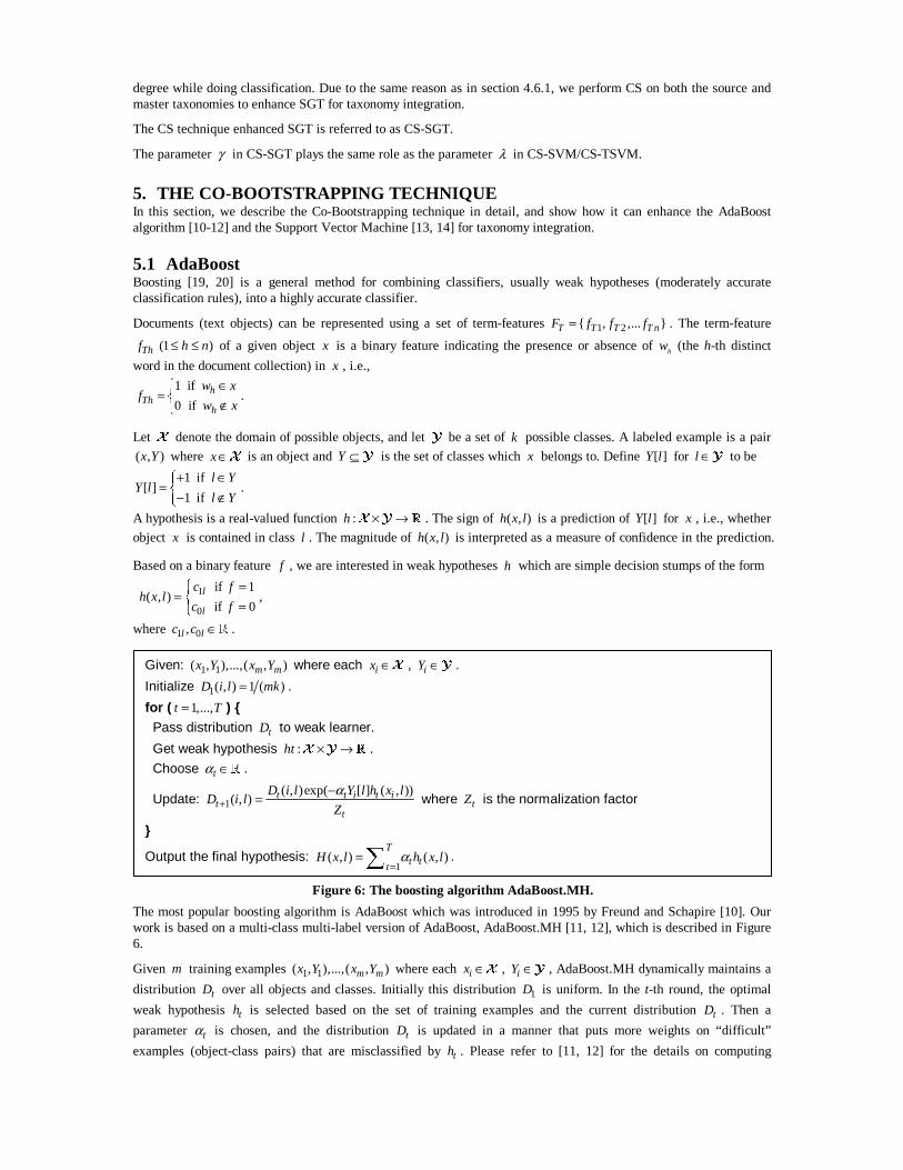
The most popular boosting algorithm is AdaBoost which was introduced in 1995 by Freund and Schapire [10]. Our work is based on a multi-class multi-label version of AdaBoost, AdaBoost.MH [11, 12], which is described in Figure 6.

Given m training examples 1 1( , ),...,( , )m mx Y x Y where each ix ∈X , iY ∈Y , AdaBoost.MH dynamically maintains a

distribution tD over all objects and classes. Initially this distribution 1D is uniform. In the t-th round, the optimal

weak hypothesis th is selected based on the set of training examples and the current distribution tD . Then a

parameter tα is chosen, and the distribution tD is updated in a manner that puts more weights on “difficult”

examples (object-class pairs) that are misclassified by th . Please refer to [11, 12] for the details on computing

Given: 1 1( , ),...,( , )m mx Y x Y where each ix ∈X , iY ∈Y .

Initialize 1( , ) 1 ( )D i l mk= .

for ( 1,...,t T= ) { Pass distribution tD to weak learner.

Get weak hypothesis :ht × → RX Y .

Choose tα ∈� .

Update: 1( , )exp( [ ] ( , ))

( , ) t t i t it

t

D i l Y l h x lD i l

Z

α+

−= where tZ is the normalization factor

}

Output the final hypothesis: 1

( , ) ( , )T

t ttH x l h x lα

==∑ .

Figure 6: The boosting algorithm AdaBoost.MH.

optimal th and tα . This procedure repeats for T rounds. The final hypothesis ( , )H x l is actually a weighted vote of

weak hypotheses 1

( , )T

t tth x lα

=∑ , and the final prediction can be computed according to the sign of ( , )H x l .

5.2 Co-Bootstrapping If we have indicator functions for each category of N, we can imagine taking those indicator functions as features

when we learn the classifier for M. This allows us to exploit the semantic relationships among the categories of M

and N without explicitly figuring out what the semantic relationships are. More specifically, for each object in M,

we augment the ordinary term-features with a set of category-features 1 2{ , ..., }NF f f f=N N N N derived from N.

The category-feature jfN (1 )j N≤ ≤ of a given object x is a binary feature indicating whether x belongs to

category jS (the j-th category of N), i.e.,

1 if

0 if

jj

j

x Sf

x S

∈⎧⎪= ⎨ ∉⎪⎩N .

In the same way, we can get a set of category-features 1 2{ , ..., }MF f f f=M M M M derived from M to be used for

supplementing the features of objects in N. The remaining problem is to obtain these indicator functions, which are

initially not available.

The Co-Bootstrapping technique overcomes the above obstacle by utilizing the bootstrapping idea, as shown in Figure

7 and 8. Let ( )r FTB denote a classifier for taxonomy T’s categorization based on feature set F at step r . Initially

we build a classifiers 0 ( )TFBN based on only term-features, then use it to classify the objects in M (the training

examples) into the categories of N, thus we can predict the value of each category-feature jf F∈N N for each object

x ∈M . At the next step we will be able to build 1 ( )TF F∪MNB using the predicted values of FN of the training

examples. Similarly we can build 0 ( )TFMB and 1 ( )TF F∪NMB . The new classifier 1 ( )TF F∪N

MB ought to be

better than 0 ( )TFBN because 1 ( )TF F∪NMB leverages more knowledge. Hence we can predict the value of each

category-feature jf F∈N N for each object x ∈M more accurately using 1 ( )TF F∪NMB instead of 0 ( )TFBN , and

afterwards we can build 2 ( )TF F∪M

NB . Also 2 ( )TF F∪MNB is very likely to be better than 1 ( )TF F∪M

NB

because 2 ( )TF F∪MNB is based on a more accurate prediction of FN . This process can be repeated iteratively in a

“ping-pong” manner. We call this technique Co-Bootstrapping6 (CB) since the two classifiers ( )r TF F∪BM N and

( )r TF F∪BN M collaborate to bootstrap themselves together.

6 This idea is named Cross-Training in [21].

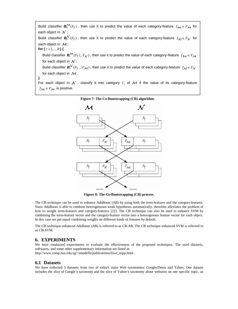
The CB technique can be used to enhance AdaBoost (AB) by using both the term-features and the category-features. Since AdaBoost is able to combine heterogeneous weak hypotheses automatically, therefore alleviates the problem of how to weight term-features and category-features [22]. The CB technique can also be used to enhance SVM by combining the term-feature vector and the category-feature vector into a heterogenous feature vector for each object. In this case we put equal combining weights on different kinds of features by default.

The CB technique enhanced AdaBoost (AB) is referred to as CB-AB. The CB technique enhanced SVM is referred to as CB-SVM.

6. EXPERIMENTS We have conducted experiments to evaluate the effectiveness of the proposed techniques. The used datasets, softwares, and some other supplementary information are listed in http://www.comp.nus.edu.sg/~smadellz/publications/ltiwt_supp.html .

6.1 Datasets We have collected 5 datasets from two of today's main Web taxonomies: Google/Dmoz and Yahoo. One dataset includes the slice of Google’s taxonomy and the slice of Yahoo’s taxonomy about websites on one specific topic, as

Build classifier 0 ( )TFBM , then use it to predict the value of each category-feature if F∈M M for

each object in N ;

Build classifier 0 ( )TFBN , then use it to predict the value of each category-feature jf F∈N N for

each object in M ; for ( 1,...,r R= ) {

Build classifier ( )r TF F∪BM N , then use it to predict the value of each category-feature if F∈M M

for each object in N ;

Build classifier ( )r TF F∪BN M , then use it to predict the value of each category-feature jf F∈N N

for each object in M ; } For each object in N , classify it into category iC of M if the value of its category-feature

if F∈M M is positive.

Figure 7: The Co-Bootstrapping (CB) algorithm.

Figure 8: The Co-Bootstrapping (CB) process.

shown in Table 1. In each slice of taxonomy, we take only the top level directories as categories, e.g., the “Movie” slice of Google’s taxonomy has categories like “Action”, “Comedy”, “Horror”, etc.

For each dataset, we show in Table 2 the number of categories occurred in Google and Yahoo respectively.

In each category, we take all items listed on the corresponding directory page and its sub-directory pages as its objects. An object (list item) corresponds to a website on the World Wide Web, which is usually described by its URL, its title, and optionally a short annotation about its content, as illustrated in Figure 9. Here each object is considered as a text document composed of its title and annotation7.

For each dataset, we show in Table 3 the number of objects occurred in Google (G), Yahoo (Y), either of them (G∪Y), and both of them (G∩Y) respectively. The set of objects in G∩Y covers only a small portion (usually less than 10%) of the set of objects in Google or Yahoo alone, which suggests the great benefit of automatically integrating them. This observation is consistent with [1].

The number of categories per object in these datasets is 1.54 on average. This observation confirms our previous statement in section 2 that an object may belong to multiple categories. Hence, multi-label classification methods and performance measures should be used.

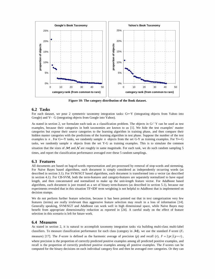
The category distributions in all theses datasets are highly skewed. For example, in Google’s Book taxonomy, the most common category contains 21% objects, but 88% categories contain fewer than 3% objects and 49% categories contain fewer than 1% objects. The category distributions of the Book dataset are shown in Figure 10. In fact, skewed category distributions have been commonly observed in real-world text categorization applications [23].

7 Note that this is different with [1, 21] which take actual Web pages as objects.

Table 3: The number of objects.

Google Yahoo G∪Y G∩Y Book 10,842 11,268 21,111 999 Disease 34,047 9,785 41,439 2,393 Movie 36,787 14,366 49,744 1,409 Music 76,420 24,518 95,971 4,967 News 31,504 19,419 49,303 1,620

Figure 9: An object (listed item) corresponds a website, which is usually described by its URL, its title, and optionally a short annotation about its content.

Table 1: The datasets.

Google Yahoo Book /Top/Shopping/Publications/Books/ /Business_and_Economy/Shopping_and_Services/Books/Bookstores/

Disease /Top/Health/Conditions_and_Diseases/ /Health/Diseases_and_Conditions/

Movie /Top/Arts/Movies/Genres/ /Entertainment/Movies_and_Film/Genres/

Music /Top/Arts/Music/Styles/ /Entertainment/Music/Genres/

News /Top/News/By_Subject/ /News_and_Media/

Table 2: The number of categories.

Google Yahoo Book 49 41 Disease 30 51 Movie 34 25 Music 47 24 News 27 34

6.2 Tasks For each dataset, we pose 2 symmetric taxonomy integration tasks: G←Y (integrating objects from Yahoo into Google) and Y←G (integrating objects from Google into Yahoo).

As stated in section 2, we formulate each task as a classification problem. The objects in G∩Y can be used as test examples, because their categories in both taxonomies are known to us [1]. We hide the test examples’ master categories but expose their source categories to the learning algorithm in training phase, and then compare their hidden master categories with the predictions of the learning algorithm in test phase. Suppose the number of the test examples is n . For G←Y tasks, we randomly sample n objects from the set G-Y as training examples. For Y←G tasks, we randomly sample n objects from the set Y-G as training examples. This is to simulate the common

situation that the sizes of M and N are roughly in same magnitude. For each task, we do such random sampling 5

times, and report the classification performance averaged over these 5 random samplings.

6.3 Features All documents are based on bag-of-words representation and pre-processed by removal of stop-words and stemming. For Naïve Bayes based algorithms, each document is simply considered as independently occurring words (as described in section 3.1). For SVM/SGT based algorithms, each document is transformed into a vector (as described in section 4.1). For CB-SVM, both the term-features and category-features are separately normalized to have equal length, and then concatenated and normalized to make up the unit-length feature vector. For AdaBoost based algorithms, each document is just treated as a set of binary term-features (as described in section 5.1), because our experiments revealed that in this situation TF×IDF term weighting is not helpful to AdaBoost that is implemented on decision stumps.

We do not perform further feature selection, because it has been pointed out that in text categorization very few features (terms) are really irrelevant thus aggressive feature selection may result in a loss of information [14]. Generally speaking, SVM/SGT and AdaBoost can work well in high dimensional space, while Naïve Bayes may benefit from appropriate dimensionality reduction as reported in [24]. A careful study on the effect of feature selection in this scenario is left for future work.

6.4 Measures As stated in section 2, it is natural to accomplish taxonomy integration tasks via building multi-class multi-label classifiers. To measure classification performance for each class (category in M), we use the standard F-score (F1

measure) [17]. The F-score is defined as the harmonic average of precision (p) and recall (r), 2 ( )F pr p r= + ,

where precision is the proportion of correctly predicted positive examples among all predicted positive examples, and recall is the proportion of correctly predicted positive examples among all positive examples. The F-scores can be computed for the binary decisions on each individual category first and then be averaged over categories. Or they can

Google's Book Taxonomy

0%

5%

10%

15%

20%

25%

0 10 20 30 40 50

category rank (from common to rare)

prop

ortio

n of

obj

ects

Yahoo's Book Taxonomy

0%

5%

10%

15%

20%

25%

0 10 20 30 40 50

category rank (from common to rare)

prop

ortio

n of

obj

ects

Figure 10: The category distribution of the Book dataset.

be computed globally over all the M n× binary decisions where M is the number of categories in consideration (the

number of categories in M) and n is the number of total test examples (the number of objects in N). The former

way is called macro-averaging and the latter way is called micro-averaging [23]. It is understood that the micro-averaged F-score (miF) tends to be dominated by the classification performance on common categories, and that the macro-averaged F-score (maF) is more influenced by the classification performance on rare categories [23]. Since the category distributions are highly skewed (see section 6.1), providing both kinds of scores is more informative than providing either alone.

6.5 Settings We use our own implementation of NB. The Lidstone’s smoothing parameter η in NB is set to an appropriate value 0.1 [16]. The performance of ENB would be greatly affected by its parameter ω . We run ENB with a series of exponentially increasing values of ω : (0, 1, 3, 10, 30, 100, 300, 1000) [1] for each taxonomy integration task, and report the best experimental results.

We use SVMlight8 [8, 14] for the implementation of SVM/TSVM. We take linear kernel, and accept all default values of parameters except “j” and “p”. The parameter “j” is set to the ratio of negative training examples over positive training examples, thus balance the cost of training errors on positive and negative examples. The parameter “p” for TSVM that means the fraction of test examples to be classified into the positive class is set to

p̂ (1 ) 0.5σ σ× + − × , where p̂ is the fraction of test examples predicted to be positive by SVM, and 0.99σ = . In all

our CS-SVM/CS-TSVM experiments, the parameter λ is set to 0.5.

We use SGTlight9 [9] for the implementation of SGT, with the following parameters: “-k 10”, “-d 100”, “-c 1000 –t f –p s”. In all our CS-SGT experiments, the parameter γ is set to 0.2.

Fine-tuning λ or γ using tune sets may generate better results than sticking with a pre-fixed value. In other words, the performance superiority of applying the CS technique is under-estimated in our experiments but performance inferiority would not be reliably established.

We use BoosTexter10 [11] for the implementation of AdaBoost. We set the boosting rounds 1000T = . BoosTexter uses only decision stumps as weak hypotheses/learners. Using more advanced learning algorithms such decision trees as weak learners in AdaBoost is likely to produce better performance..

The Co-Bootstrapping iteration number is set to 8R = for both CB-AB and CB-SVM experiments.

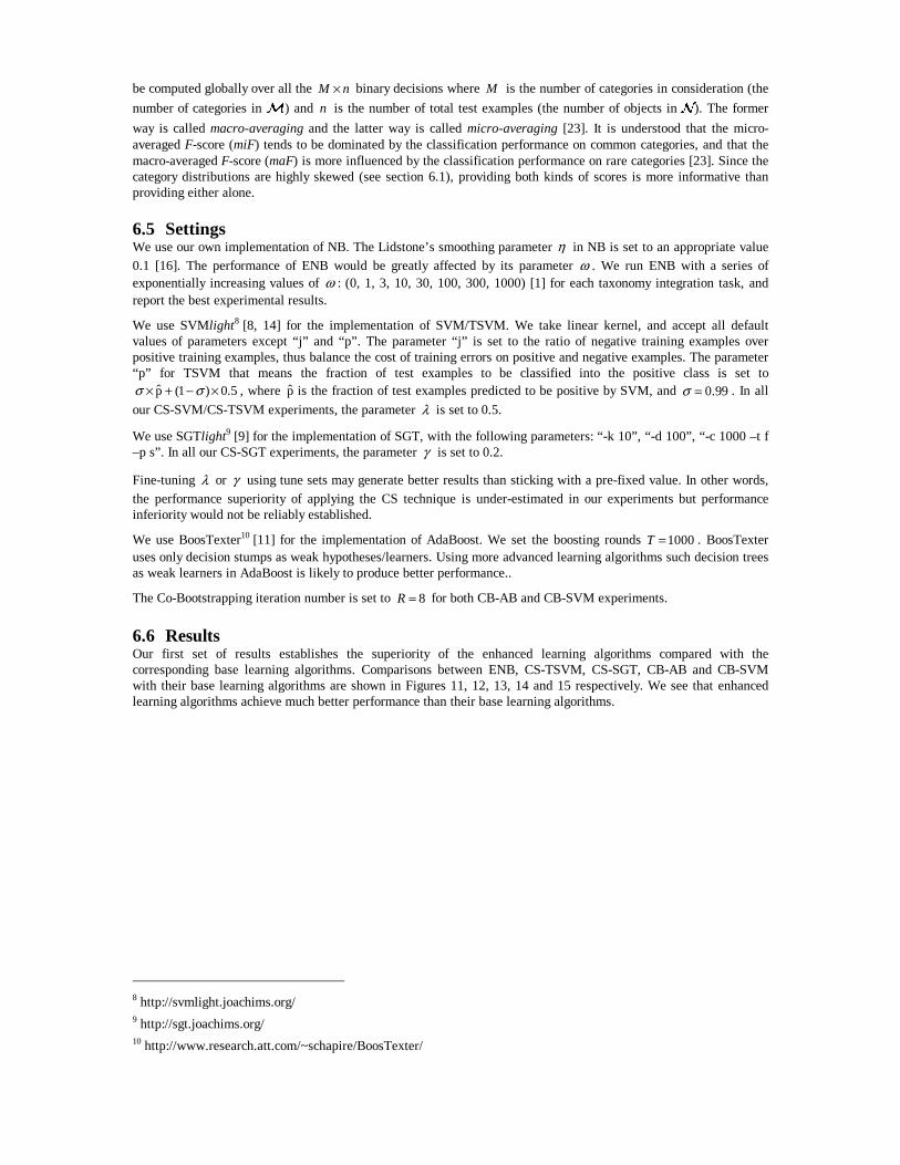
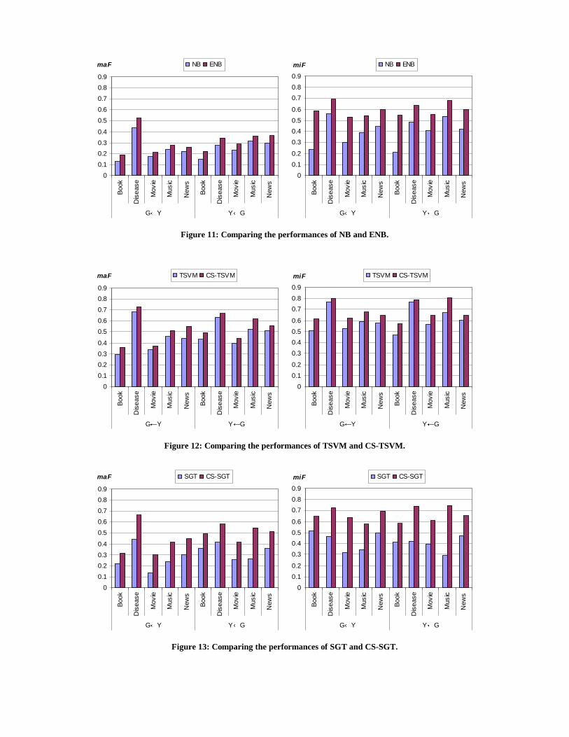
6.6 Results Our first set of results establishes the superiority of the enhanced learning algorithms compared with the corresponding base learning algorithms. Comparisons between ENB, CS-TSVM, CS-SGT, CB-AB and CB-SVM with their base learning algorithms are shown in Figures 11, 12, 13, 14 and 15 respectively. We see that enhanced learning algorithms achieve much better performance than their base learning algorithms.

8 http://svmlight.joachims.org/ 9 http://sgt.joachims.org/ 10 http://www.research.att.com/~schapire/BoosTexter/

0

0.1

0.2

0.3

0.4

0.5

0.6

0.7

0.8

0.9

Boo

k

Dis

ease

Mov

ie

Mus

ic

New

s

Boo

k

Dis

ease

Mov

ie

Mus

ic

New

s

G←Y Y←G

maF SGT CS-SGT

0

0.1

0.2

0.3

0.4

0.5

0.6

0.7

0.8

0.9

Boo

k

Dis

ease

Mov

ie

Mus

ic

New

s

Boo

k

Dis

ease

Mov

ie

Mus

ic

New

s

G←Y Y←G

miF SGT CS-SGT

Figure 13: Comparing the performances of SGT and CS-SGT.

0

0.1

0.2

0.3

0.4

0.5

0.6

0.7

0.8

0.9

Boo

k

Dis

ease

Mov

ie

Mus

ic

New

s

Boo

k

Dis

ease

Mov

ie

Mus

ic

New

s

G←Y Y←G

maF TSVM CS-TSVM

0

0.1

0.2

0.3

0.4

0.5

0.6

0.7

0.8

0.9

Boo

k

Dis

ease

Mov

ie

Mus

ic

New

s

Boo

k

Dis

ease

Mov

ie

Mus

ic

New

s

G←Y Y←G

miF TSVM CS-TSVM

Figure 12: Comparing the performances of TSVM and CS-TSVM.

0

0.1

0.2

0.3

0.4

0.5

0.6

0.7

0.8

0.9

Boo

k

Dis

ease

Mov

ie

Mus

ic

New

s

Boo

k

Dis

ease

Mov

ie

Mus

ic

New

s

G←Y Y←G

maF NB ENB

0

0.1

0.2

0.3

0.4

0.5

0.6

0.7

0.8

0.9

Boo

k

Dis

ease

Mov

ie

Mus

ic

New

s

Boo

k

Dis

ease

Mov

ie

Mus

ic

New

s

G←Y Y←G

miF NB ENB

Figure 11: Comparing the performances of NB and ENB.

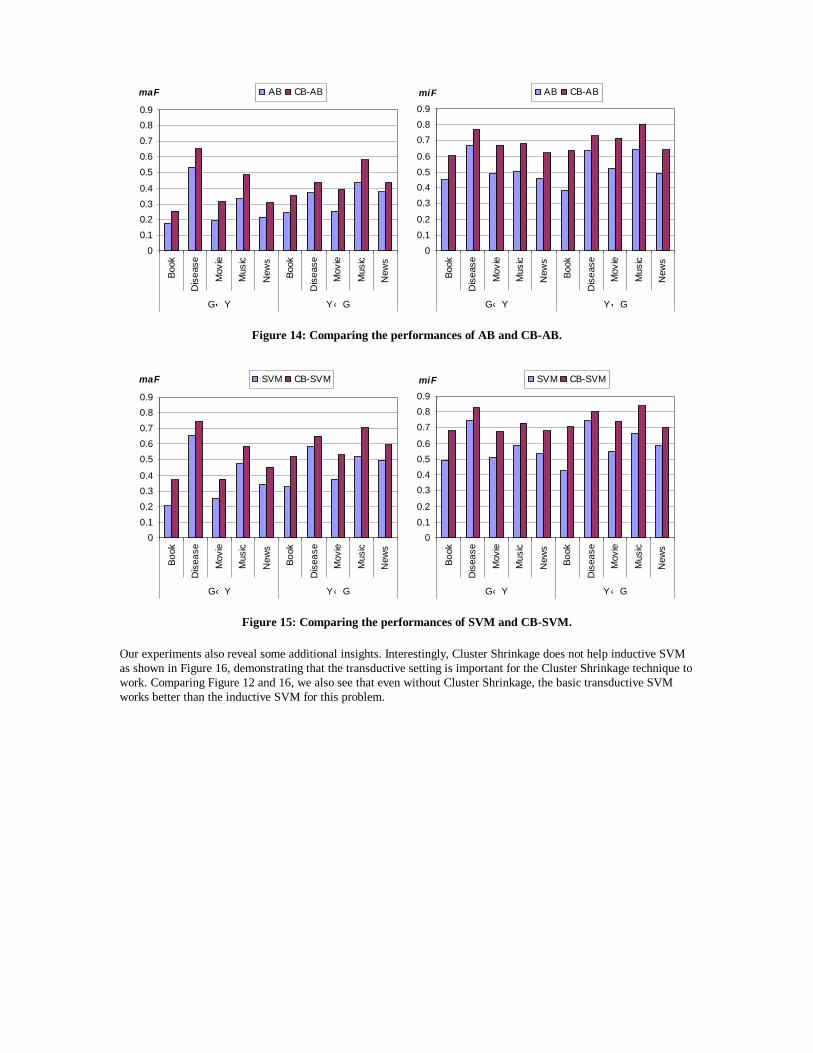
Our experiments also reveal some additional insights. Interestingly, Cluster Shrinkage does not help inductive SVM as shown in Figure 16, demonstrating that the transductive setting is important for the Cluster Shrinkage technique to work. Comparing Figure 12 and 16, we also see that even without Cluster Shrinkage, the basic transductive SVM works better than the inductive SVM for this problem.

0

0.1

0.2

0.3

0.4

0.5

0.6

0.7

0.8

0.9

Boo

k

Dis

ease

Mov

ie

Mus

ic

New

s

Boo

k

Dis

ease

Mov

ie

Mus

ic

New

s

G←Y Y←G

maF SVM CB-SVM

0

0.1

0.2

0.3

0.4

0.5

0.6

0.7

0.8

0.9

Boo

k

Dis

ease

Mov

ie

Mus

ic

New

s

Boo

k

Dis

ease

Mov

ie

Mus

ic

New

s

G←Y Y←G

miF SVM CB-SVM

Figure 15: Comparing the performances of SVM and CB-SVM.

0

0.1

0.2

0.3

0.4

0.5

0.6

0.7

0.8

0.9

Boo

k

Dis

ease

Mov

ie

Mus

ic

New

s

Boo

k

Dis

ease

Mov

ie

Mus

ic

New

s

G←Y Y←G

maF AB CB-AB

0

0.1

0.2

0.3

0.4

0.5

0.6

0.7

0.8

0.9

Boo

k

Dis

ease

Mov

ie

Mus

ic

New

s

Boo

k

Dis

ease

Mov

ie

Mus

ic

New

s

G←Y Y←G

miF AB CB-AB

Figure 14: Comparing the performances of AB and CB-AB.

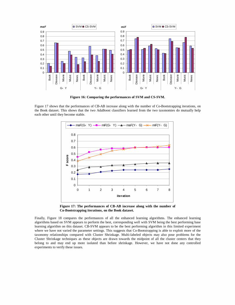
Figure 17 shows that the performances of CB-AB increase along with the number of Co-Bootstrapping iterations, on the Book dataset. This shows that the two AdaBoost classifiers learned from the two taxonomies do mutually help each other until they become stable.

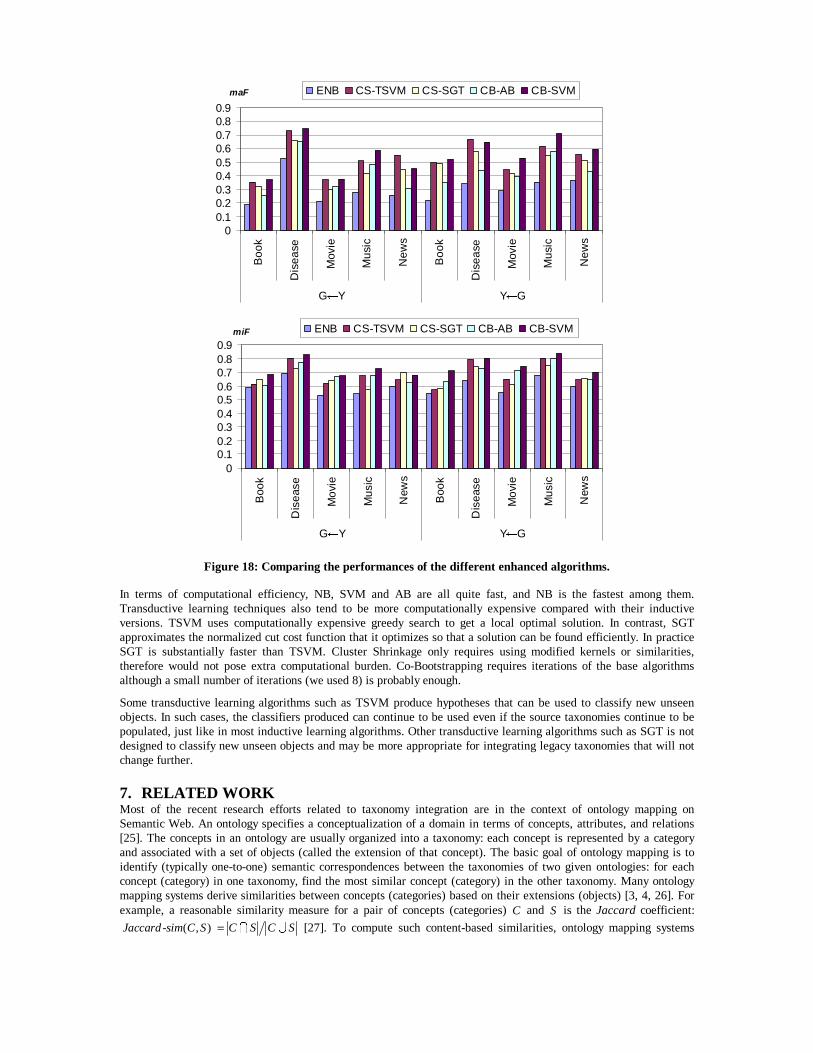
Finally, Figure 18 compares the performances of all the enhanced learning algorithms. The enhanced learning algorithms based on SVM appears to perform the best, corresponding well with SVM being the best performing base learning algorithm on this dataset. CB-SVM appears to be the best performing algorithm in this limited experiment where we have not varied the parameter settings. This suggests that Co-Bootstrapping is able to exploit more of the taxonomy relationships compared with Cluster Shrinkage. Multi-labeled objects may also pose problems for the Cluster Shrinkage techniques as these objects are drawn towards the midpoint of all the cluster centers that they belong to and may end up more isolated than before shrinkage. However, we have not done any controlled experiments to verify these issues.

0

0.1

0.2

0.3

0.4

0.5

0.6

0.7

0.8

0.9

Boo

k

Dis

ease

Mov

ie

Mus

ic

New

s

Boo

k

Dis

ease

Mov

ie

Mus

ic

New

s

G←Y Y←G

maF SVM CS-SVM

0

0.1

0.2

0.3

0.4

0.5

0.6

0.7

0.8

0.9

Boo

k

Dis

ease

Mov

ie

Mus

ic

New

s

Boo

k

Dis

ease

Mov

ie

Mus

ic

New

s

G←Y Y←G

miF SVM CS-SVM

Figure 16: Comparing the performances of SVM and CS-SVM.

0

0.1

0.2

0.3

0.4

0.5

0.6

0.7

0.8

0 1 2 3 4 5 6 7 8

iteration

F s

core

maF(G←Y) miF(G←Y) maF(Y←G) miF(Y←G)

Figure 17: The performances of CB-AB increase along with the number of Co-Bootstrapping iterations, on the Book dataset.

In terms of computational efficiency, NB, SVM and AB are all quite fast, and NB is the fastest among them. Transductive learning techniques also tend to be more computationally expensive compared with their inductive versions. TSVM uses computationally expensive greedy search to get a local optimal solution. In contrast, SGT approximates the normalized cut cost function that it optimizes so that a solution can be found efficiently. In practice SGT is substantially faster than TSVM. Cluster Shrinkage only requires using modified kernels or similarities, therefore would not pose extra computational burden. Co-Bootstrapping requires iterations of the base algorithms although a small number of iterations (we used 8) is probably enough.

Some transductive learning algorithms such as TSVM produce hypotheses that can be used to classify new unseen objects. In such cases, the classifiers produced can continue to be used even if the source taxonomies continue to be populated, just like in most inductive learning algorithms. Other transductive learning algorithms such as SGT is not designed to classify new unseen objects and may be more appropriate for integrating legacy taxonomies that will not change further.

7. RELATED WORK Most of the recent research efforts related to taxonomy integration are in the context of ontology mapping on Semantic Web. An ontology specifies a conceptualization of a domain in terms of concepts, attributes, and relations [25]. The concepts in an ontology are usually organized into a taxonomy: each concept is represented by a category and associated with a set of objects (called the extension of that concept). The basic goal of ontology mapping is to identify (typically one-to-one) semantic correspondences between the taxonomies of two given ontologies: for each concept (category) in one taxonomy, find the most similar concept (category) in the other taxonomy. Many ontology mapping systems derive similarities between concepts (categories) based on their extensions (objects) [3, 4, 26]. For example, a reasonable similarity measure for a pair of concepts (categories) C and S is the Jaccard coefficient:

- ( , )Jaccard sim C S C S C S= ∩ ∪ [27]. To compute such content-based similarities, ontology mapping systems

00.10.20.30.40.50.60.70.80.9

Boo

k

Dis

ease

Mov

ie

Mus

ic

New

s

Boo

k

Dis

ease

Mov

ie

Mus

ic

New

s

G←Y Y←G

maF ENB CS-TSVM CS-SGT CB-AB CB-SVM

00.10.20.30.40.50.60.70.80.9

Boo

k

Dis

ease

Mov

ie

Mus

ic

New

s

Boo

k

Dis

ease

Mov

ie

Mus

ic

New

s

G←Y Y←G

miF ENB CS-TSVM CS-SGT CB-AB CB-SVM

Figure 18: Comparing the performances of the different enhanced algorithms.

need to first integrate objects from one taxonomy into the other and vice versa, i.e., do taxonomy integration. So our work can be used for this kind of content-based ontology mapping.

As stated in section 2, taxonomy integration can be formulated as a classification problem. The Rocchio algorithm [17, 28] has been applied to this problem in [3]; and the Naïve Bayes (NB) algorithm [5] has been applied to this problem in [4], without exploiting information in the source taxonomies.

In [1], Agrawal and Srikant proposed the Enhanced Naïve Bayes (ENB) approach to taxonomy integration, which we have analyzed in depth and compared with our proposed approaches. In [21], Sarawagi, Chakrabarti and Godboley independently proposed the Co-Bootstrapping technique (which they named Cross-Training) to enhance SVM for taxonomy integration, as well as an Expectation Maximization (EM) based approach EM2D (2-Dimensional Expectation Maximization).

In [22], AdaBoost is selected as the framework to combine term-features and automatically extracted semantic-features in the context of text categorization. We also choose AdaBoost to combine heterogeneous features (term-features and category-features), but it is for a different problem (taxonomy integration) and it works in a different way (Co-Bootstrapping).

Recently there has been considerable interest in learning from a small number of labeled examples together with a large number of unlabeled examples. This is called semi-supervised learning. Representative works on this topic include employing the Expectation Maximization (EM) technique [29] and Co-Training [30-33]. Basically Co-Training attempts to utilize unlabeled data to help classification through exploiting a particular form of redundancy in data: each object is described by multiple views (disjoint feature sets) which are compatible and uncorrelated (conditionally independent) [30]. Co-Bootstrapping is similar to Co-Training in the sense that both techniques iteratively train two classifiers which mutually reinforce each other. Nevertheless, Co-Bootstrapping and Co-Training are essentially targeted for different kinds of problems, as shown in Table 5.

8. HIERARCHICAL TAXONOMIES AND OTHER EXTENSIONS As most taxonomies are hierarchical in nature, it would be important to extend the techniques proposed in this paper to handle hierarchical taxonomies effectively. Although it is possible to flatten the hierarchy to a single level, past studies have shown that exploiting the hierarchical structure can lead to better classification results [34, 35]. While we have not investigated techniques of incorporating the information in the hierarchies, it is possible to suggest various simple extensions to the current techniques.

To handle hierarchies in SVM/TSVM, it is possible to use the technique proposed in [35]. One could also incorporate a hierarchical version of Cluster Shrinkage that is similar to the idea explored in [36]: transforming each object’s position to a weighted average of its original position, its parent-cluster’s center, its grandparent-cluster’s center, …, all the way up to the root. For example, consider a two-level taxonomy H where jkS is a sub-category of jS .

Suppose the center of jkS is jkc and the center of jS is jc . For each ik iS S∈ ⊂x , one reasonable way to achieve

hierarchical CS is as follows: first compute (1 )ik i ikµ µ′ = + −c c c using a parameter 0 1µ≤ ≤ , and then replace x

with (1 )ikλ λ′ ′= + −x c x using a parameter 0 1λ≤ ≤ .

To extend Co-Bootstrapping, it is useful to consider hierarchies as trees. One simple technique to exploit the hierarchy in Co-Bootstrapping would then be to include indicator functions for both internal and leaf nodes, where the indicator function for an internal node would indicate whether the object belongs to the subtree rooted at that internal node. This allows the learning algorithm to also exploit relationships between subtrees in the taxonomies

Table 5: Comparison between Co-Training and Co-Bootstrapping.

Co-Training Co-Bootstrapping

Classes One set of classes. Two sets of classes: (1) the set of source categories ; (2) the set of master categories.

Features Two disjoint sets of features: V1 and V2.

Two sets of features: (1) conventional-features plus source category-features; (2) conventional-features plus master category-features;

Assumption V1 and V2 are compatible and uncorrelated (conditionally independent).

The source and master taxonomies have some semantic overlap, i.e., they are somewhat correlated.

rather than just between leaves. Assuming that each internal node has more than one child, the number of indicator functions used will be at most two times the number of indicator functions used in the non-hierarchical technique as the number of internal nodes is always less than the number of leaves.

Many issues remain to be explored. Even within these algorithms, there are variations that we have not experimented with, such as combining transductive learning algorithms with Co-Bootstrapping. We also do not yet have a good characterization of when the techniques work (c.f. compatibility and conditional independence conditions in Co-Training).

9. CONCLUSION The problem itself, learning to integrate taxonomies, has been considered before in [1] that is also described as the starting point of the current investigation. The general idea is to use machine learning algorithms to automatically map objects from one taxonomy (more specifically, a set of classes) into another one. The intended application, taxonomy integration, is one of the key challenges for creating the Semantic Web.

Our main contributions in this paper are to propose and investigate two techniques, Cluster Shrinkage and Co-Bootstrapping, that can effectively enhance conventional machine learning algorithms for taxonomy integration by exploiting the background knowledge about how objects are classified in the source taxonomy. Cluster Shrinkage biases the learning algorithms against splitting source categories and works for algorithms that are based on the distance/similarity between objects. Our experiments indicate that it works well only when transductive learning algorithms such as the Transductive Support Vector Machine or Spectral Graph Transducer are used. Co-Bootstrapping tries to facilitate the exploitation of relationships between source and master categories by providing class indicator functions as additional features for the objects. This technique works for any learning algorithm that can utilize indicator features and appears to be able to exploit more semantic relationships between the taxonomies compared with Cluster Shrinkage. While Cluster Shrinkage still takes a rather “asymmetrical” view as ENB with a clear distinction between source and master classifications, Co-Bootstrapping takes a “symmetrical” view, relying on a Co-Training like idea of two classifications informing each other. The experiments show that both techniques can improve the base learning algorithms substantially. The experiments also suggest that Co-Bootstrapping with Support Vector Machines works the best although more work will have to be done before definitive conclusions can be drawn.

10. ACKNOWLEDGMENTS We would like to thank the anonymous reviewers for their helpful comments and many useful suggestions.

11. REFERENCES [1] R. Agrawal and R. Srikant, "On Integrating Catalogs," in Proceedings of the 10th International World Wide Web

Conference (WWW). Hong Kong, 2001, pp. 603-612. [2] T. Berners-Lee, J. Hendler, and O. Lassila, "The Semantic Web," in Scientific American, 2001. [3] M. S. Lacher and G. Groh, "Facilitating the Exchange of Explicit Knowledge through Ontology Mappings," in

Proceedings of the Fourteenth International Florida Artificial Intelligence Research Society Conference (FLAIRS). Key West, FL, 2001, pp. 305-309.

[4] A. Doan, J. Madhavan, P. Domingos, and A. Halevy, "Learning to Map between Ontologies on the Semantic Web," in Proceedings of the 11th International World Wide Web Conference (WWW). Hawaii, USA, 2002, pp. 662-673.

[5] T. Mitchell, Machine Learning, international ed. New York: McGraw Hill, 1997. [6] V. N. Vapnik, Statistical Learning Theory. New York, NY: Wiley, 1998. [7] K. Bennett, "Combining Support Vector and Mathematical Programming Methods for Classification," in

Advances in Kernel Methods -Support Vector Learning, B. Scholkopf, C. Burges, and A. Smola, Eds.: MIT-Press, 1999.

[8] T. Joachims, "Transductive Inference for Text Classification using Support Vector Machines," in Proceedings of the 16th International Conference on Machine Learning (ICML). Bled, Slovenia, 1999, pp. 200-209.

[9] T. Joachims, "Transductive Learning via Spectral Graph Partitioning," in Proceedings of the 20th International Conference on Machine Learning (ICML). Washington DC, USA, 2003, pp. 290-297.

[10] Y. Freund and R. E. Schapire, "A Decision-theoretic Generalization of On-line Learning and an Application to Boosting," Journal of Computer and System Sciences, vol. 55, pp. 119-139, 1997.

[11] R. E. Schapire and Y. Singer, "BoosTexter: A Boosting-based System for Text Categorization," Machine Learning, vol. 39, pp. 135-168, 2000.

[12] R. E. Schapire and Y. Singer, "Improved Boosting Algorithms Using Confidence-rated Predictions," Machine Learning, vol. 37, pp. 297-336, 1999.

[13] N. Cristianini and J. Shawe-Taylor, An Introduction to Support Vector Machines. Cambridge, UK: Cambridge University Press, 2000.

[14] T. Joachims, "Text Categorization with Support Vector Machines: Learning with Many Relevant Features," in Proceedings of the 10th European Conference on Machine Learning (ECML). Chemnitz, Germany, 1998, pp. 137-142.

[15] A. McCallum and K. Nigam, "A Comparison of Event Models for Naive Bayes Text Classification," in AAAI-98 Workshop on Learning for Text Categorization. Madison, WI, 1998, pp. 41-48.

[16] R. Agrawal, R. Bayardo, and R. Srikant, "Athena: Mining-based Interactive Management of Text Databases," in Proceedings of the 7th International Conference on Extending Database Technology (EDBT). Konstanz, Germany, 2000, pp. 365-379.

[17] R. Baeza-Yates and B. Ribeiro-Neto, Modern Information Retrieval. New York, NY: Addison-Wesley, 1999. [18] V. N. Vapnik, The Nature of Statistical Learning Theory, 2nd ed. New York, NY: Springer-Verlag, 2000. [19] R. E. Schapire, "The Boosting Approach to Machine Learning: An Overview," in MSRI Workshop on Nonlinear

Estimation and Classification. Berkeley, CA, 2002. [20] R. Meir and G. Ratsch, "An Introduction to Boosting and Leveraging," in Advanced Lectures on Machine

Learning, LNCS, S. Mendelson and A. J. Smola, Eds.: Springer-Verlag, 2003, pp. 119-184. [21] S. Sarawagi, S. Chakrabarti, and S. Godbole, "Cross-Training: Learning Probabilistic Mappings between

Topics," in Proceedings of the 9th ACM SIGKDD International Conference on Knowledge Discovery and Data Mining (KDD). Washington DC, USA, 2003, pp. 177-186.

[22] L. Cai and T. Hofmann, "Text Categorization by Boosting Automatically Extracted Concepts," in Proceedings of the 26th Annual International ACM SIGIR Conference on Research and Development in Information Retrieval (SIGIR). Toronto, Canada, 2003, pp. 182-189.

[23] Y. Yang and X. Liu, "A Re-examination of Text Categorization Methods," in Proceedings of the 22nd ACM International Conference on Research and Development in Information Retrieval (SIGIR). Berkeley, CA, 1999, pp. 42-49.

[24] D. Mladenic, "Turning Yahoo to Automatic Web-Page Classifier," in Proceedings of the 13th European Conference on Artificial Intelligence (ECAI). Brighton, UK, 1998, pp. 473-474.

[25] D. Fensel, Ontologies: A Silver Bullet for Knowledge Management and Electronic Commerce: Springer-Verlag, 2001.

[26] R. Ichise, H. Takeda, and S. Honiden, "Rule Induction for Concept Hierarchy Alignment," in Proceedings of the Workshop on Ontologies and Information Sharing at the 17th International Joint Conference on Artificial Intelligence (IJCAI). Seattle, WA, 2001, pp. 26-29.

[27] C. J. v. Rijsbergen, Information Retrieval, 2nd ed. London, UK: Butterworths, 1979. [28] J. J. Rocchio, "Relevance Feedback in Information Retrieval," in The SMART Retrieval System: Experiments in

Automatic Document Processing, G. Salton, Ed.: Prentice-Hall, 1971, pp. 313-323. [29] K. Nigam, A. McCallum, S. Thrun, and T. Mitchell, "Text Classification from Labeled and Unlabeled

Documents using EM," Machine Learning, vol. 39, pp. 103-134, 2000. [30] A. Blum and T. Mitchell, "Combining Labeled and Unlabeled Data with Co-Training," in Proceedings of the

11th Annual Conference on Computational Learning Theory (COLT). Madison, WI, 1998, pp. 92-100. [31] M. Collins and Y. Singer, "Unsupervised Models for Named Entity Classification," in Proceedings of the Joint

SIGDAT Conference on Empirical Methods in Natural Language Processing and Very Large Corpora (EMNLP). College Park, MD, 1999, pp. 189-196.

[32] K. Nigam and R. Ghani, "Analyzing the Effectiveness and Applicability of Co-training," in Proceedings of the 9th International Conference on Information and Knowledge Management (CIKM). McLean, VA, 2000, pp. 86-93.

[33] U. Brefeld and T. Scheffer, "Co-EM Support Vector Learning," in Proceedings of the 21st International Conference on Machine Learning (ICML). Banff, Alberta, Canada, 2004.

[34] S. Chakrabarti, B. Dom, R. Agrawal, and P. Raghavan, "Using Taxonomy, Discriminants, and Signatures for Navigating in Text Databases," in Proceedings of the 23rd International Conference on Very Large Data Bases (VLDB). Athens, Greece, 1997, pp. 446-455.

[35] S. Dumais and H. Chen, "Hierarchical Classification of Web Content," in Proceedings of the 23rd Annual International ACM SIGIR Conference on Research and Development in Information Retrieval (SIGIR). Athens, Greece, 2000, pp. 256-263.

[36] A. McCallum, R. Rosenfeld, T. Mitchell, and A. Y. Ng, "Improving Text Classification by Shrinkage in a Hierarchy of Classes," in Proceedings of the 15th International Conference on Machine Learning (ICML). Madison, WI, 1998, pp. 359-367.

Dell Zhang is a research fellow in the National University of Singapore (NUS) under the Singapore-MIT Alliance (SMA). He has received his BEng and PhD in Computer Science from the Southeast University, Nanjing, China. His primary research interests include machine learning, data mining and information retrieval.

Wee Sun Lee is an Associate Professor at the Department of Computer Science, National University of Singapore (NUS), and a Fellow of the Singapore-MIT Alliance (SMA). He obtained his Bachelor of Engineering degree in Computer Systems Engineering from the University of Queensland in 1992, and his PhD from the Department of Systems Engineering at the Australian National University in 1996. He is interested in computational learning theory, machine learning and information retrieval.