learning to optimize via posterior sampling arxiv:1301.2609v5 … · russo and van roy: learning to...

MATHEMATICS OF OPERATIONS RESEARCHVol. 00, No. 0, Xxxxx 0000, pp. 000–000

issn 0364-765X |eissn 1526-5471 |00 |0000 |0001

INFORMSdoi 10.1287/xxxx.0000.0000

c© 0000 INFORMS

Authors are encouraged to submit new papers to INFORMS journals by means ofa style file template, which includes the journal title. However, use of a templatedoes not certify that the paper has been accepted for publication in the named jour-nal. INFORMS journal templates are for the exclusive purpose of submitting to anINFORMS journal and should not be used to distribute the papers in print or onlineor to submit the papers to another publication.

Learning to Optimize Via Posterior Sampling

Daniel RussoDepartment of Management Science and Engineering, Stanford University, Stanford, California, 94305, [email protected]

Benjamin Van RoyDepartments of Management Science and Engineering and Electrical Engineering, Stanford University, Stanford, California,

94305, [email protected]

This paper considers the use of a simple posterior sampling algorithm to balance between exploration andexploitation when learning to optimize actions such as in multi-armed bandit problems. The algorithm, alsoknown as Thompson Sampling and as probability matching, offers significant advantages over the popularupper confidence bound (UCB) approach, and can be applied to problems with finite or infinite actionspaces and complicated relationships among action rewards. We make two theoretical contributions. Thefirst establishes a connection between posterior sampling and UCB algorithms. This result lets us convertregret bounds developed for UCB algorithms into Bayesian regret bounds for posterior sampling. Our secondtheoretical contribution is a Bayesian regret bound for posterior sampling that applies broadly and can bespecialized to many model classes. This bound depends on a new notion we refer to as the eluder dimension,which measures the degree of dependence among action rewards. Compared to UCB algorithm Bayesianregret bounds for specific model classes, our general bound matches the best available for linear modelsand is stronger than the best available for generalized linear models. Further, our analysis provides insightinto performance advantages of posterior sampling, which are highlighted through simulation results thatdemonstrate performance surpassing recently proposed UCB algorithms.

Key words : online optimization; multi–armed bandits; Thompson samplingMSC2000 subject classification : Primary: 93E35; secondary: 62L05OR/MS subject classification : Primary: decision analysis: sequential;History : Received February 26, 2013; revised November 21, 2013

1. Introduction. We consider an optimization problem faced by an agent who is uncertainabout how his actions influence performance. The agent selects actions sequentially, and upon eachaction observes a reward. A reward function governs the mean reward of each action. The agentrepresents his initial beliefs through a prior distribution over reward functions. As rewards areobserved the agent learns about the reward function, and this allows him to improve his behavior.Good performance requires adaptively sampling actions in a way that strikes an effective balancebetween exploring poorly understood actions and exploiting previously acquired knowledge toattain high rewards. In this paper, we study a simple algorithm for selecting actions and providefinite time performance guarantees that apply across a broad class of models.

The problem we study has attracted a great deal of recent interest and is often referred to asthe multi-armed bandit (MAB) problem with dependent arms. We refer to the problem as one oflearning to optimize to emphasize its divergence from the classical MAB literature. In the typicalMAB framework, there are a finite number of actions that are modeled independently; samplingone action provides no information about the rewards that can be gained through selecting other

1

arX

iv:1

301.

2609

v5 [

cs.L

G]

3 F

eb 2

014

mailto:[email protected]

mailto:[email protected]

Russo and Van Roy: Learning to Optimize Via Posterior Sampling2 Mathematics of Operations Research 00(0), pp. 000–000, c© 0000 INFORMS

actions. In contrast, we allow for infinite action spaces and for general forms of model uncer-tainty, captured by a prior distribution over a set of possible reward functions. Recent papershave addressed this problem in cases where the relationship among action rewards takes a knownparametric form. For example, Abbasi-Yadkori et al. [2], Dani et al. [17], Rusmevichientong andTsitsiklis [31] study the case where actions are described by a finite number of features and thereward function is linear in these features. Other authors have studied cases where the rewardfunction is Lipschitz continuous [13, 23, 36], sampled from a Gaussian process [35], or takes theform of a generalized [18] or sparse [3] linear model.

Each paper cited above studies an upper confidence bound (UCB) algorithm. Such an algorithmforms an optimistic estimate of the mean-reward value for each action, taking it to be the high-est statistically plausible value. It then selects an action that maximizes among these optimisticestimates. Optimism encourages selection of poorly-understood actions, which leads to informativeobservations. As data accumulates, optimistic estimates are adapted, and this process of explo-ration and learning converges toward optimal behavior.

We study an alternative algorithm that we refer to as posterior sampling. It is also also knownas Thompson sampling and as probability matching. The algorithm randomly selects an actionaccording to the probability it is optimal. Although posterior sampling was first proposed almosteighty years ago, it has until recently received little attention in the literature on multi-armedbandits. While its asymptotic convergence has been established in some generality [30], not muchelse is known about its theoretical properties in the case of dependent arms, or even in the case ofindependent arms with general prior distributions. Our work provides some of the first theoreticalguarantees.

Our interest in posterior sampling is motivated by several potential advantages over UCB algo-rithms, which we highlight in Section 4.3. While particular UCB algorithms can be extremelyeffective, performance and computational tractability depends critically on the confidence sets usedby the algorithm. For any given model, there is a great deal of design flexibility in choosing thestructure of these sets. Because posterior sampling avoids the need for confidence bounds, its usegreatly simplifies the design process and admits practical implementations in cases where UCBalgorithms are computationally onerous. In addition, we show through simulations that posteriorsampling outperforms various UCB algorithms that have been proposed in the literature.

In this paper, we make two theoretical contributions. The first establishes a connection betweenposterior sampling and UCB algorithms. In particular, we show that while the regret of a UCBalgorithm can be bounded in terms of the confidence bounds used by the algorithm, the Bayesianregret of posterior sampling can be bounded in an analogous way by any sequence of confidencebounds. In this sense, posterior sampling preserves many of the appealing theoretical propertiesof UCB algorithms without requiring explicit, designed, optimism. We show that, due to this con-nection, existing analysis available for specific UCB algorithms immediately translates to Bayesianregret bounds for posterior sampling.

Our second theoretical contribution is a Bayesian regret bound for posterior sampling that appliesbroadly and can be specialized to many specific model classes. Our bound depends on a new notionof dimension that measures the degree of dependence among actions. We compare our notion ofdimension to the Vapnik-Chervonenkis dimension and explain why that and other measures ofdimension used in the supervised learning literature do not suffice when it comes to analyzingposterior sampling.

The remainder of this paper is organized as follows. The next section discusses related literature.Section 3 then provides a formal problem statement. We describe UCB and posterior samplingalgorithms in Section 4. We then establish in Section 5 a connection between them, which we applyin Section 6 to convert existing bounds for UCB algorithms to bounds for posterior sampling.Section 7 develops a new notion of dimension and presents Bayesian regret bounds that depend onit. Section 8 presents simulation results. A closing section makes concluding remarks.

Russo and Van Roy: Learning to Optimize Via Posterior SamplingMathematics of Operations Research 00(0), pp. 000–000, c© 0000 INFORMS 3

2. Related Literature. One distinction of results presented in this paper is that they centeraround Bayesian regret as a measure of performance. In the next subsection, we discuss this choiceand how it relates to performance measures used in other work. Following that, we review priorresults and their relation to results of this paper.

2.1. Measures of Performance. Several recent papers have established theoretical resultson posterior sampling. One difference between this work and ours is that we focus on a differentmeasure of performance. These papers all study the algorithm’s regret, which measures its cumu-lative loss relative to an algorithm that always selects the optimal action, for some fixed rewardfunction. To derive these bounds, each paper fixes an uninformative prior distribution with a con-venient analytic structure, and studies posterior sampling assuming this particular prior is used.With one exception [6], the focus is on the classical multiarmed bandit problem, where samplingone action provides no information about others.

Posterior sampling can be applied to a much broader class of problems, and one of its greateststrengths is its ability to incorporate prior knowledge in a flexible and coherent way. We thereforeaim to develop results that accommodate the use of a wide range of models. Accordingly, most ofour results allow for an arbitrary prior distribution over a particular class of mean reward functions.In order to derive meaningful results at this level of generality, we study the algorithm’s expectedregret, where the expectation is taken with respect to the prior distribution over reward functions.This quantity is sometimes called the algorithm’s Bayesian regret. We find this to be a practicallyrelevant measure of performance and find this choice allows for more elegant analysis. Further, aswe discuss in Section 3, the Bayesian regret bounds we provide in some cases immediately yieldregret bounds.

In addition, studying Bayesian regret reveals deep connections between posterior sampling andthe principle of optimism in the face of uncertainty, which we feel provides new conceptual insightinto the algorithm’s performance. Optimism in the face of uncertainty is a general principle andis not inherently tied to any measure of performance. Indeed, algorithms based on this principlehave been shown to be asymptotically efficient in terms of both regret [26] and Bayesian regret[25], to satisfy order optimal minimax regret bounds [8], to satisfy order optimal bounds on regretand Bayesian regret when the reward function is linear [31], and to satisfy strong bounds whenthe reward function is sampled from a Gaussian process prior [35]. We take a very general viewof optimistic algorithms, allowing upper confidence bounds to be constructed in an essentiallyarbitrary way based on the algorithm’s observations and possibly the prior distribution over rewardfunctions.

2.2. Related Results. Though it was first proposed in 1933, posterior sampling has untilrecently received relatively little attention. Interest in the algorithm grew after empirical studies[15, 34] demonstrated performance exceeding state-of-the-art methods. An asymptotic convergenceresult was established by May et al. [30], but finite time guarantees remain limited. The developmentof further performance bounds was raised as an open problem at the 2012 Conference on LearningTheory [28].

Three recent papers [4, 5, 22] provide regret bounds for posterior sampling when applied to MABproblems with finitely many independent actions and rewards that follow Bernoulli processes. Theseresults demonstrate that posterior sampling is asymptotically optimal for the class of problemsconsidered. A key feature of the bounds is their dependence on the difference between the optimaland second-best mean-reward values. Such bounds tend not to be meaningful when the numberof actions is large or infinite unless they can be converted to bounds that are independent of thisgap, which is sometimes the case.

In this paper, we establish distribution-independent bounds. When the action space A is finite,we establish a finite time Bayesian regret bound of order

√|A|T logT . This matches what is


implied by the analysis of Agrawal and Goyal [5]. However, our bound does not require actions aremodeled independently, and our approach also leads to meaningful bounds for problems with largeor infinite action sets.

Only one other paper has studied posterior sampling in a context involving dependent actions[6]. That paper considers a contextual bandit model with arms whose mean-reward values aregiven by a d-dimensional linear model. The cumulative T -period regret is shown to be of orderd2

ε

√T 1+ε ln(Td) ln 1

δwith probability at least 1 − δ. Here ε ∈ (0,1) is a parameter used by the

algorithm to control how quickly the posterior distribution concentrates. The Bayesian regretbounds we will establish are stronger than those implied by the results of Agrawal and Goyal [6].In particular, we provide a Bayesian regret bound of order d

√T lnT that holds for any compact

set of actions. This is order–optimal up to a factor of lnT [31].We are also the first to establish finite time performance bounds for several other problem classes.

One applies to linear models when the vector of coefficients is likely to be sparse; this boundis stronger than the aforementioned one that applies to linear models in the absence of sparsityassumptions. We establish the the first bounds for posterior sampling when applied to generalizedlinear models and to problems with a general Gaussian prior. Finally, we establish bounds thatapply very broadly and depend on a new notion of dimension.

Unlike most of the relevant literature, we study MAB problems in a general framework, allowingfor complicated relationships between the rewards generated by different actions. The closest relatedwork is that of Amin et al. [7], who consider the problem of learning the optimum of a functionthat lies in a known, but otherwise arbitrary set of functions. They provide bounds based on anew notion of dimension, but unfortunately this notion does not provide a bound for posteriorsampling. Other work provides general bounds for contextual bandit problems where the contextspace is allowed to be infinite, but the action space is small (see, e.g., [10]). Our model capturescontextual bandits as a special case, but we emphasize problem instances with large or infiniteaction sets, and where the goal is to learn without sampling every possible action.

A focus of our paper is the connection between posterior sampling and UCB approaches. Wediscuss UCB algorithms in some detail in Section 4. UCB algorithms have been the primaryapproach considered in the segment of the stochastic MAB literature that treats models withdependent arms. Other approaches are the knowledge gradient algorithm [32], forced explorationschemes for linear bandits [1, 16, 31], and exponential-weighting schemes [10].

There is an immense and rapidly growing literature on bandits with independent arms and onadversarial bandits. Theoretical work on stochastic bandits with independent arms often focuseson UCB algorithms [9, 26] or on the Gittin’s index approach [20]. Bubeck and Cesa-Bianchi [11]provide a review of work on UCB algorithms and on adversarial bandits. Gittins et al. [19] coverwork on Gittin’s indices and related extensions.

Since an initial version of this paper was made publicly available, the literature on the analysisof posterior sampling has rapidly grown. Korda et al. [24] extend their earlier work [22] to thecase where reward distributions lie in the 1–dimensional exponential family. Bubeck and Liu [12]combine the regret decomposition we derive in Section 5 with the confidence bound analysis ofAudibert and Bubeck [8] to tighten the bound provided in Section 6.1, and also consider a problemsetting where the regret of posterior sampling is bounded uniformly over time. Li [29] explores aconnection between posterior sampling and exponential weighting schemes, and Gopalan et al. [21]study the asymptotic growth rate of regret in problems with dependent arms.

3. Problem Formulation. We consider a model involving a set of actions A and a set ofreal-valued functions F = fρ :A 7→R|ρ ∈Θ, indexed by a parameter that takes values from anindex set Θ. We will define random variables with respect to a probability space (Ω,F,P). A randomvariable θ indexes the true reward function fθ. At each time t, the agent is presented with a possiblyrandom subset At ⊆A and selects an action At ∈At, after which she observes a reward Rt.


We denote by Ht the history (A1,A1,R1, . . . ,At−1,At−1,Rt−1,At) of observations available tothe agent when choosing an action At. The agent employs a policy π = πt|t ∈ N, which is adeterministic sequence of functions, each mapping the history Ht to a probability distribution overactions A. For each realization of Ht, πt(Ht) is a distribution over A with support At, thoughwith some abuse of notation, we will often write this distribution as πt. The action At is selectedby sampling from the distribution πt, so that P(At ∈ ·|πt) = P(At ∈ ·|Ht) = πt(·). We assume thatE[Rt|Ht, θ,At] = fθ(At). In other words, the realized reward is the mean-reward value corrupted byzero-mean noise. We will also assume that for each f ∈F and t∈N, arg maxa∈At f(a) is nonemptywith probability one, though algorithms and results can be generalized to handle cases where thisassumption does not hold.

The T -period regret of a policy π is the random variable defined by

Regret (T, π, θ) =T∑t=1

E[

maxa∈At

fθ(a)− fθ (At)

∣∣∣∣ θ] .The T -period Bayesian regret is defined by E [Regret (T, π, θ)], where the expectation is taken withrespect to the prior distribution over θ. Hence,

BayesRegret (T, π) =T∑t=1

E[maxa∈At

fθ(a)− fθ (At)

].

This quantity is also called Bayes risk, or simply expected regret.Remark 1. Measurability assumptions are required for the above expectations to be well-

defined. In order to avoid technicalities that do not present fundamental obstacles in the contextswe consider, we will not explicitly address measurability issues in this paper and instead simplyassume that functions under consideration satisfy conditions that ensure relevant expectations arewell-defined.Remark 2. All equalities between random variables in this paper hold almost surely with

respect to the underlying probability space.

3.1. On Regret and Bayesian Regret. To interpret results about the regret and Bayesianregret of various algorithms and to appreciate their practical implications, it is useful to takenote of several properties of and relationships between these performance measures. For starters,asymptotic bounds on Bayesian regret are essentially asymptotic bounds on regret. In partic-ular, if BayesRegret(T,π) = O(g(T )) for some non-negative function g then an application ofMarkov’s inequality shows Regret(T,π, θ) =OP (g(T )). Here OP indicates that Regret(T,π, θ)/g(T )is stochastically bounded under the prior distribution. In other words, for all ε > 0 there existsM > 0 such that

P(

Regret(T,π, θ)

g(T )≥M

)≤ ε ∀T ∈N.

This observation can be further extended to establish a sense in which Bayesian regret is robust toprior mis-specification. In particular, if the agent’s prior over θ is µ but for convenience he selectsactions as though his prior were an alternative µ, the resulting Bayesian regret satisfies

Eθ0∼µ [Regret(T,π, θ0)]≤∥∥∥∥dµdµ

∥∥∥∥µ,∞

Eθ0∼µ [Regret(T,π, θ0)] ,

where dµ/dµ is the Radon-Nikodym derivative1 of µ with respect to µ and ‖ · ‖µ,∞ is the essentialsupremum magnitude with respect to µ. Note that the final term on the right-hand-side is theBayesian regret for a problem with prior µ without mis-specification.

1 Note that the Radon-Nikodym derivative is only well defined when µ is absolutely continuous with respect to µ.


It is also worth noting that an algorithm’s Bayesian regret can only differ significantly from itsworst-case regret if regret varies significantly depending on the realization of θ. This provides onemethod of converting Bayesian regret bounds to regret bounds. For example, consider the linearmodel fθ(a) = θTφ(a) where Θ =

ρ∈Rd : ‖ρ‖2 = S

is the boundary of a hypersphere in Rd. Let

At =A for each t and let the set of feature vectors be φ(a)|a∈A=u∈Rd| ‖u‖2 ≤ 1

. Consider

a problem instance where θ is uniformly distributed over Θ, and the noise terms Rt − fθ(At) areindependent of θ. By symmetry, the regret of most reasonable algorithms for this problem shouldbe the same for all realizations of θ, and indeed this is the case for posterior sampling. Therefore,in this setting Bayesian regret is equal to worst–case regret. This view also suggests that in orderto attain strong minimax regret bounds, one should not choose a uniform prior as in Agrawal andGoyal [5], but should instead place more prior weight on the worst possible realizations of θ (seethe discussion of “least favorable” prior distributions in Lehmann and Casella [27]).

3.2. On Changing Action Sets. Our stochastic model of action sets At is distinct relativeto most of the multi-armed bandit literature, which assumes that At =A. This construct allowsour formulation to address a variety of practical issues that are usually viewed as beyond the scopeof standard multi-armed bandit formulations. Let us provide three examples.Example 1. Contextual Models. The contextual multi-armed bandit model is a special case

of the formulation presented above. In such a model, an exogenous Markov process Xt takingvalues in a set X influences rewards. In particular, the expected reward at time t is given byfθ(a,Xt). However, this is mathematically equivalent to a problem with stochastic time-varyingdecision sets At. In particular, one can define the set of actions to be the set of state-action pairsA := (x, a) : x∈A, a∈A(x), and the set of available actions to be At = (Xt, a) : a∈A(Xt).Example 2. Cautious Actions. In some applications, one may want to explore without

risking terrible performance. This can be accomplished by restricting the set At to conservativeactions. Then, the instantaneous regret in our framework is the gap between the reward from thechosen action and the reward from the best conservative action. In many settings, the Bayesianregret bounds we will establish for posterior sampling imply that the algorithm either attainsnear-optimal performance or converges to a point where any better decision is unacceptably risky.

A number of formulations of this flavor are amenable to efficient implementations of PosteriorSampling. For example, consider a problem where A is a polytope or ellipsoid in Rd and fθ(a) =〈a, θ〉. Suppose θ has a Gaussian prior and that reward noise is Gaussian. Then, the posterior dis-tribution of θ is Gaussian. Consider an ellipsoidal confidence set Ut =

u | ‖u−µt‖Σt ≤ β

, for some

scalar constant β > 0, where µt and Σt are the mean and covariance matrix of θ, conditioned onHt. One can attain good worst-case performance with high probability by solving the robust opti-mization problem Vrobust ≡maxa∈Aminu∈Ut 〈a,u〉, which is a tractable linear saddle-point problem.Letting our cautious set be given by

At =

a∈A |min

u∈Ut〈a,u〉 ≥ Vrobust−α

for some scalar constant α > 0, we can then select an optimal cautious action given θ by solvingmaxa∈At 〈a, θ〉, which is equivalent to

maximize 〈a, θ〉subject to a∈A

‖a‖Σ−1t≤ 1

β(〈a,µt〉−Vrobust +α) .

This problem is computationally tractable, which accommodates efficient implementation of pos-terior sampling.


Example 3. Adaptive Adversaries. Consider a model in which rewards are influenced bythe choices of an adaptive adversary. At each time period, the adversary selects an action A−t fromsome set A− based on past observations. The agent observes this action, responds with an actionA+t selected from a set A+, and receives a reward that depends on the pair of actions (A+

t ,A−t ).

This fits our framework if the action At is taken to be the pair (A+t ,A

−t ), and the set of actions

available to the agent is At = (a,A−t )|a∈A+.

4. Algorithms. We will establish finite time performance bounds for posterior sampling byleveraging prior results pertaining to UCB algorithms and a connection we will develop betweenthe two classes of algorithms. To set the stage for our analysis, we discuss the algorithms in thissection.

4.1. UCB Algorithms. UCB algorithms have received a great deal of attention in the MABliterature. Such an algorithm makes use of a sequence of upper confidence bounds U = Ut|t∈N,each of which is a function that takes the history Ht as its argument. For each realization ofHt, Ut(Ht) is a function mapping A to R. With some abuse of notation, we will often write thisfunction as Ut and its value at a ∈ A as Ut(a). The upper confidence bound Ut(a) representsthe greatest value of fθ(a) that is statistically plausible given Ht. A UCB algorithm selects anaction At ∈ arg maxa∈At Ut(a) that maximizes the upper confidence bound. We will assume thatthe argmax operation breaks ties among optima in a deterministic way. As such, each action isdetermined by the history Ht, and for the policy π= πt|t∈N followed by a UCB algorithm, eachaction distribution πt concentrates all probability on a single action.

As a concrete example, consider Algorithm 1, proposed by Auer et al. [9] to address MABproblems with a finite number of independent actions. For such problems, At =A, θ is a vectorwith one independent component per action, and the reward function is given by fθ(a) = θa.The algorithm begins by selecting each action once. Then, for each subsequent time t > |A|, thealgorithm generates point estimates of action rewards, defines upper confidence bounds based onthem, and selects actions accordingly. For each action a, the point estimate θt(a) is taken to be theaverage reward obtained from samples of action a taken prior to time t. The upper confidence boundis produced by adding an “uncertainty bonus” β

√log t/Nt(a) to the point estimate, where Nt(a) is

the number of times action a was selected prior to time t and β is an algorithm parameter generallyselected based on reward variances. This uncertainty bonus leads to an optimistic assessment ofexpected reward when there is uncertainty, and it is this optimism that encourages explorationthat reduces uncertainty. As Nt(a) increases, uncertainty about action a diminishes and so does theuncertainty bonus. The log t term ensures that the agent does not permanently rule out any action,which is important as there is always some chance of obtaining an overly pessimistic estimate byobserving an unlikely sequence of rewards.

Our second example treats a linear bandit problem. Here we assume θ is drawn from a normaldistribution N(µ0,Σ0) but without assuming that the covariance matrix is diagonal. We considera linear reward function fθ(a) = 〈φ(a), θ〉 and assume the reward noise Rt − fθ(At) is normallydistributed and independent from (Ht,At, θ). One can show that, conditioned on the history Ht,θ remains normally distributed. Algorithm 2 presents an implementation of UCB algorithm forthis problem. The expectations can be computed efficiently via Kalman filtering. The algorithmemploys upper confidence bound 〈φ(a), µt〉 + β log(t)‖φ(a)‖Σt . The term ‖φ(a)‖Σt captures theposterior variance of θ in the direction φ(a), and, as with the case of independent arms, causes theuncertainty bonus β log(t)‖φ(a)‖Σt to diminish as the number of observations increases.

4.2. Posterior Sampling. The posterior sampling algorithm simply samples each actionaccording to the probability it is optimal. In particular, the algorithm applies action sampling dis-tributions πt = P (A∗t ∈ · |Ht), where A∗t is a random variable that satisfies A∗t ∈ arg maxa∈At fθ(a).


Algorithm 1 Independent UCB

1: Initialize: Select each action once2: Update Statistics: For each a∈A,θt(a)← sample average of observed rewardsNt(a)← number of times a sampled so far

3: Select Action:Atarg max

a∈A

θt(a) +β

√log tNt(a)

4: Increment t and Goto Step 2

Algorithm 2 Linear–Gaussian UCB

1: Update Statistics:µt←E[θ|Ht]Σt←E[(θ−µt)(θ−µt)>|Ht]

2: Select Action:At ∈ arg max

a∈A

〈φ(a), µt〉+β log(t)‖φ(a)‖Σt


Practical implementations typically operate by, at each time t, sampling an index θt ∈Θ from thedistribution P (θ ∈ · |Ht) and then generating an action At ∈ arg maxa∈At fθt(a). To illustrate, letus provide concrete examples that address problems analogous to Algorithms 1 and 2.

Our first example involves a model with independent arms. In particular, suppose θ is drawnfrom a normal distribution N(µ0,Σ0) with a diagonal covariance matrix Σ0, the reward functionis given by fθ(a) = θa, and the reward noise Rt− fθ(At) is normally distributed and independentfrom (Ht,At, θ). It then follows that, conditioned on the history Ht, θ remains normally distributedwith independent components. Algorithm 3 presents an implementation of posterior sampling forthis problem. The expectations are easy to compute and can also be computed recursively.

Our second example treats a linear bandit problem. Algorithm 4 presents a posterior samplinganalogue to Algorithm 2. As before, we assume θ is drawn from a normal distribution N(µ0,Σ0).We consider a linear reward function fθ(a) = 〈φ(a), θ〉 and assume the reward noise Rt− fθ(At) isnormally distributed and independent from (Ht,At, θ).

Algorithm 3Independent Posterior Sampling

1: Sample Model:θt ∼N(µt−1,Σt−1)

2: Select Action:At ∈ arg maxa∈A θt(a)

3: Update Statistics: For each a,µta←E[θa|Ht]Σtaa←E[(θa−µta)2|Ht]


Algorithm 4Linear Posterior Sampling

1: Sample Model:θt ∼N(µt−1,Σt−1)

2: Select Action:At ∈ arg maxa∈A〈φ(a), θt〉

3: Update Statistics:µt←E[θ|Ht]Σt←E[(θ−µt)(θ−µt)>|Ht]


4.3. Potential Advantages of Posterior Sampling. Well designed optimistic algorithmscan be extremely effective. When simple and efficient UCB algorithms are available, they maybe preferable to posterior sampling. Our work is primarily motivated by the challenges in design-ing optimistic algorithms to address very complicated problems, and the important advantagesposterior sampling sometimes offers in such cases.

The performance of a UCB algorithm depends critically on the choice of upper confidence bounds(Ut : t∈N). These functions should be chosen so that Ut(A

∗)≥ fθ(A∗) with high probability. How-ever, unless the posterior distribution of fθ(a) can be expressed in closed form, computing highquantiles of this distribution can require extensive Monte Carlo simulation for each possible action.


In addition, since A∗ depends on θ, it isn’t even clear that Ut(a) should be set to a particular quan-tile of the posterior distribution of fθ(a). Strong frequentist upper confidence bounds were recentlydeveloped [14] for problems with independent arms, but it is often unclear how to generate tightconfidence sets for more complicated models. In fact, even in the case of a linear model, the designof confidence sets has required sophisticated tools from the study of multivariate self-normalizedmartingale processes [2]. We believe posterior sampling provides a powerful tool for practitioners,as a posterior sampling approach can be designed for complicated models without sophisticatedstatistical analysis. Further, posterior sampling does not require computing posterior distributionsbut only sampling from posterior distributions. As such, Markov chain Monte Carlo methods canoften be used to efficiently generate samples even when the posterior distribution is complex.

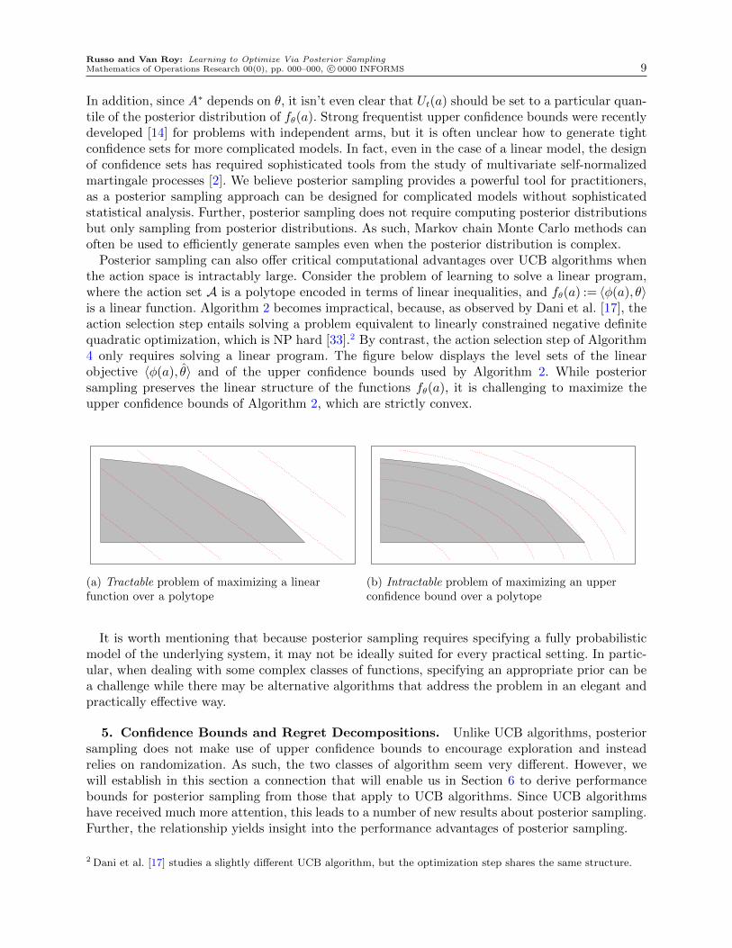
Posterior sampling can also offer critical computational advantages over UCB algorithms whenthe action space is intractably large. Consider the problem of learning to solve a linear program,where the action set A is a polytope encoded in terms of linear inequalities, and fθ(a) := 〈φ(a), θ〉is a linear function. Algorithm 2 becomes impractical, because, as observed by Dani et al. [17], theaction selection step entails solving a problem equivalent to linearly constrained negative definitequadratic optimization, which is NP hard [33].2 By contrast, the action selection step of Algorithm4 only requires solving a linear program. The figure below displays the level sets of the linearobjective 〈φ(a), θ〉 and of the upper confidence bounds used by Algorithm 2. While posteriorsampling preserves the linear structure of the functions fθ(a), it is challenging to maximize theupper confidence bounds of Algorithm 2, which are strictly convex.

(a) Tractable problem of maximizing a linearfunction over a polytope

(b) Intractable problem of maximizing an upperconfidence bound over a polytope

It is worth mentioning that because posterior sampling requires specifying a fully probabilisticmodel of the underlying system, it may not be ideally suited for every practical setting. In partic-ular, when dealing with some complex classes of functions, specifying an appropriate prior can bea challenge while there may be alternative algorithms that address the problem in an elegant andpractically effective way.

5. Confidence Bounds and Regret Decompositions. Unlike UCB algorithms, posteriorsampling does not make use of upper confidence bounds to encourage exploration and insteadrelies on randomization. As such, the two classes of algorithm seem very different. However, wewill establish in this section a connection that will enable us in Section 6 to derive performancebounds for posterior sampling from those that apply to UCB algorithms. Since UCB algorithmshave received much more attention, this leads to a number of new results about posterior sampling.Further, the relationship yields insight into the performance advantages of posterior sampling.

2 Dani et al. [17] studies a slightly different UCB algorithm, but the optimization step shares the same structure.


5.1. UCB Regret Decomposition. Consider a UCB algorithm with an upper confidencebound sequence U = Ut|t ∈ N. Recall that At ∈ arg maxa∈At Ut(a) and A∗t ∈ arg maxa∈At fθ(a).We have the following simple regret decomposition:

fθ (A∗t )− fθ(At)

= fθ (A∗t )−Ut(At) +Ut(At)− fθ(At)

≤ [fθ (A∗t )−Ut(A∗t )] +[Ut(At)− fθ

(At)]. (1)

The inequality follows from the fact that At is chosen to maximize Ut. If the upper confidencebound is an upper bound with high probability, as one would expect from a UCB algorithm, thenthe first term is negative with high probability. The second term, Ut(At)−fθ

(At), penalizes for the

width of the confidence interval. As actions are sampled Ut should diminish and converge on fθ.As such, both terms of the decomposition should eventually vanish. An important feature of thisdecomposition is that, so long as the first term is negative, it bounds regret in terms of uncertaintyabout the current action At.

Taking the expectation of (1) establishes that the T -period Bayesian regret of a UCB algorithmsatisfies

BayesRegret(T, πU

)≤E

T∑t=1

[Ut(At)− fθ(At)

]+E

T∑t=1

[fθ (A∗t )−Ut(A∗t )] , (2)

where πU is the policy derived from U .

5.2. Posterior Sampling Regret Decomposition. As established by the following propo-sition, the Bayesian regret of posterior sampling decomposes in a way analogous to what we haveshown for UCB algorithms. Recall that, with some abuse of notation, for an upper confidence boundsequence Ut|t∈N we denote by Ut(a) the random variable Ut(Ht)(a). The following propositionallows Ut to be an arbitrary real valued function of Ht and a∈A. Let πPS denote the policy followedby posterior sampling.

Proposition 1. For any upper confidence bound sequence Ut|t∈N,

BayesRegret(T, πPS

)=E

T∑t=1

[Ut(At)− fθ(At)] +ET∑t=1

[fθ (A∗t )−Ut(A∗t )] , (3)

for all T ∈N.

Proof. Note that, conditioned on Ht, the optimal action A∗t and the action At selected byposterior sampling are identically distributed, and Ut is deterministic. Hence, E [Ut(A

∗t ) |Ht] =

E [Ut(At) |Ht]. Therefore

E [fθ(A∗t )− fθ (At)] = E [E [fθ(A

∗t )− fθ (At) |Ht]]

= E [E [Ut (At)−Ut (A∗t ) + fθ(A∗t )− fθ (At) |Ht]]

= E [E [Ut(At)− fθ(At) |Ht] +E [fθ (A∗t )−Ut(A∗t ) |Ht]]= E [Ut(At)− fθ(At)] +E [fθ (A∗t )−Ut(A∗t )] .

Summing over t gives the result. To compare (2) and (3) consider the case where fθ takes values in [0, C]. Then,

BayesRegret(T, πU

)≤E

T∑t=1

[Ut(At)− fθ(At)

]+C

T∑t=1

P (fθ (A∗t )>Ut(A∗t ))

and

BayesRegret(T, πPS

)≤E

T∑t=1

[Ut(At)− fθ(At)] +CT∑t=1

P (fθ (A∗t )>Ut(A∗t )) .


An important difference to take note of is that the Bayesian regret bound of πU depends on thespecific upper confidence bound sequence U used by the UCB algorithm in question whereas thebound of πPS applies simultaneously for all upper confidence bound sequences. This suggests that,while the Bayesian regret of a UCB algorithm depends critically on the specific choice of confidencesets, posterior sampling depends on the best possible choice of confidence sets. This is a crucialadvantage when there are complicated dependencies among actions, as designing and computingwith appropriate confidence sets presents significant challenges. This difficulty is likely the mainreason that posterior sampling significantly outperforms recently proposed UCB algorithms in thesimulations presented in Section 8.

We have shown how upper confidence bounds characterize Bayesian regret bounds for posteriorsampling. We will leverage this concept in the next two sections. Let us emphasize, though, thatwhile our analysis of posterior sampling will make use of upper confidence bounds, the actualperformance of posterior sampling does not depend on upper confidence bounds used in the analysis.

6. From UCB to Posterior Sampling Regret Bounds. In this section we presentBayesian regret bounds for posterior sampling that can be derived by combining our regret decom-position (3) with results from prior work on UCB regret bounds. Each UCB regret bound wasestablished through a common procedure, which entailed specifying lower and upper confidencebounds Lt :A 7→ R and Ut :A 7→ R so that Lt(a)≤ fθ(a)≤ Ut(a) with high probability for each tand a, and then providing an expression that dominates the sum

∑T

1 (Ut−Lt)(at) for all sequencesof actions a1, .., aT . As we will show, each such analysis together with our regret decomposition (3)leads to a Bayesian regret bound for posterior sampling.

6.1. Finitely Many Actions. We consider in this section a problem with |A|<∞ actionsand rewards satisfying Rt ∈ [0,1] for all t almost surely. We note, however, that the results wediscuss can be extended to cases where Rt is not bounded but where instead its distribution is“light-tailed.” It is also worth noting that we make no further assumptions on the class of rewardfunctions F or on the prior distribution over θ.

In this setting, Algorithm 1, which was proposed by Auer et al. [9], is known to satisfy aproblem-independent regret bound of order

√|A|T logT . Under an additional assumption that

action rewards are independent and take values in 0,1, an order√|A|T logT regret bound for

posterior sampling is also available [5].Here we provide a Bayesian regret bound that is also of order

√|A|T logT but does not require

that action rewards are independent or binary. Our analysis, like that of Auer et al. [9], makes useof confidence sets that are Cartesian products of action-specific confidence intervals. The regretdecomposition (3) lets us use such confidence sets to produce bounds for posterior sampling evenwhen the algorithm itself may exploit dependencies among actions.

Proposition 2. If |A|=K <∞ and Rt ∈ [0,1], then for any T ∈N

BayesRegret(T,πPS)≤ 2minK,T+ 4√KT (2 + 6 log(T )). (4)

Proof. Let Nt(a) =∑t

l=1 1(At = a) denote the number of times a is sampled over the first tperiods, and µt(a) = Nt(a)−1

∑t

l=1 1(At = a)Rt denote the empirical average reward from thesesamples. Define upper and lower confidence bounds as follows:

Ut(a) = min

µt−1(a) +

√2 + 6 log(T )

Nt−1(a),1

Lt(a) = max

µt−1(a)−

√2 + 6 log(T )

Nt−1(a),0

. (5)

The next lemma, which is a consequence of analysis in Abbasi-Yadkori et al. [2], shows these holdwith high probability. Were actions sampled in an iid fashion, this lemma would follow immediatelyfrom the Hoeffding inequality. For more details, see Appendix A.


Lemma 1. If Ut(a) and Lt(a) are defined as in (5), then P(⋃T

t=1fθ(a) /∈ [Lt(a),Ut(a)])≤

1/T .

First consider the case where T ≤K. Since fθ(a)∈ [0,1], BayesRegret(T,πPS)≤ T = minK,T.Now, assume T >K. Then,

BayesRegret(T,πPS) ≤ E

[T∑t=1

(Ut−Lt)(At)

]+TP

(⋃a∈A

T⋃t=1

fθ(a) /∈ [Lt(a),Ut(a)]

)

≤ E

[T∑t=1

(Ut−Lt)(At)

]+K.

We now turn to bounding∑T

t=1(Ut − Lt)(At). Let Ta = t≤ T :At = a denote the periods in

which a is selected. Then,∑T

t=1(Ut−Lt)(At) =∑

a∈A∑

t∈Ta(Ut−Lt)(a). We show,

∑t∈Ta

(Ut−Lt)(a)≤ 1 + 2√

2 + 6 log(T )∑t∈Ta

(1 +Nt−1(a))−1/2 = 1 + 2√

2 + 6 log(T )

NT (a)−1∑j=0

(j+ 1)−1/2

andNT (a)−1∑j=0

(j+ 1)−1/2 ≤NT (a)∫x=0

x−1/2dx= 2√NT (a).

Summing over actions and applying the cauchy-shwartz inequality yields,

BayesRegret(T,πPS)≤ 2K + 4√

2 + 6 log(T )∑a∈A

√NT (a)

(a)

≤ 2K + 4

√(2 + 6 log(T ))K

∑a

NT (a)

= 2K + 4√KT (2 + 6 log(T ))

(b)= 2minK,T+ 4

√KT (2 + 6 log(T )),

where (a) follows from the cauchy-shwartz inequality and (b) follows from the assumption thatT >K.

6.2. Linear and Generalized Linear Models. We now consider function classes that rep-resent linear and generalized linear models. The bound of Proposition 2 applies so long as thenumber of actions is finite, but we will establish alternative bounds that depend on the dimensionof the function class rather than the number of actions. Such bounds accommodate problems withinfinite action sets and can be much stronger than the bound of Proposition 2 if there are manyactions.

The Bayesian regret bounds we provide in this section derive from regret bounds of the UCBliterature. In Section 7, we will establish a Bayesian regret bound that is as strong for the case oflinear models and stronger for the case of generalized linear models. Since the results of Section 7to a large extent supersede those we present here, we aim to be brief and avoid formal proofs inthis section’s discussion of the bounds and how they follow from results in the literature.

6.2.1. Linear Models In the “linear bandit” problem studied by [2, 3, 17, 31], reward func-tions are parameterized by a vector θ ∈Θ⊂Rd, and there is a known feature mapping φ :A 7→Rdsuch that fθ(a) = 〈φ(a), θ〉. The following proposition establishes Bayesian regret bounds for suchproblems. The proposition uses the term σ-sub-Gaussian to describe any random variable X thatsatisfies E exp(λX)≤ exp(λ2σ2/2) for all λ∈R.


Proposition 3. Fix positive constants σ, c1, and c2. If Θ ⊂ Rd, fθ(a) = 〈φ(a), θ〉 for someφ :A 7→ R, supρ∈Θ ‖ρ‖2 ≤ c1, and supa∈A ‖φ(a)‖2 ≤ c2, and for each t, Rt − fθ(At) conditioned on(Ht,At, θ) is σ-sub-Gaussian, then

BayesRegret(T, πPS

)=O(d logT

√T ),

and

BayesRegret(T, πPS

)= O

(E√‖θ‖0 dT

).

The second bound essentially replaces the dependence on the dimension d with one on E√‖θ‖0 d.

The “zero-norm” ‖θ‖0 is the number of nonzero components, which can be much smaller than dwhen the reward function admits a sparse representation. Note that O ignores logarithmic factors.Both bounds follow from our regret decomposition (3) together with the analysis of [2], in the caseof the first bound, and the analysis of [3], in the case of the second bound. We now provide a briefsketch of how these bounds can be derived.

If fθ takes values in [−C, C] then (3) implies

BayesRegret(T, πPS

)≤E

T∑t=1

[Ut(At)−Lt(At)]+2CT∑t=1

[P (fθ(A∗t )>Ut(A

∗t )) +P (fθ(At)<Lt(At))] .

(6)The analyses of [2] and [3] follow two steps that can be used to bound the right hand side ofthis equation. In the first step, an ellipsoidal confidence set Θt := ρ ∈ Rd : ‖ρ− θt‖Vt ≤

√βt is

constructed, where for some λ∈R, Vt :=∑t

k=1 φ(At)φ(At)T +λI captures the amount of exploration

carried out in each direction up to time t. The upper and lower bounds induced by the ellipsoid areUt(a) := maxC,maxρ∈Θt (ρTφ(a)) and Lt(a) := min−C,minρ∈Θt (ρTφ(a)). If the sequence ofconfidence parameters β1, . . . , βT is selected so that P(θ /∈Θt|Ht)≤ 1/T then the second term of theregret decomposition is less than 4C. For these confidence sets, the second step establishes a boundon∑T

1 (Ut−Lt)(at) that holds for any sequence of actions. The analyses presented on pages 7-8 of[17] and pages 14-15 of [2] each implies such a bound of order

√dmaxt≤T βtT log(T/λ). Plugging

in closed form expressions for βt provided in these papers leads to the bounds of Proposition 3.

6.2.2. Generalized Linear Models In a generalized linear model, the reward function takesthe form fθ(a) := g (〈φ(a), θ 〉) where the inverse link function g is strictly increasing and contin-uously differentiable. The analysis of [18] can be applied to establish a Bayesian regret bound forposterior sampling, but with one caveat. The algorithm considered in [18] begins by selecting asequence of actions a1, .., ad with linearly independent feature vectors φ(a1), . . . , φ(ad). Until now,we haven’t even assumed such actions exist or that they are guaranteed to be feasible over thefirst d time periods. After this period of designed exploration, the algorithm selects at each timean action that maximizes an upper confidence bound. What we will establish using the resultsfrom [18] is a bound on a similarly modified version of posterior sampling, in which the first dactions taken are a1, . . . , ad, while subsequent actions are selected by posterior sampling. Note thatthe posterior distribution employed at time d+ 1 is conditioned on observations made over thefirst d time periods. We denote this modified posterior sampling algorithm by πIPS

a1,...,ad. It is worth

mentioning here that in Section 7 we present a result with a stronger bound that applies to thestandard version of posterior sampling, which does not include a designed exploration period.

Proposition 4. Fix positive constants c1, c2, C, and λ. If Θ ⊂ Rd, fθ(a) = g(〈φ(a), θ〉)for some strictly increasing continuously differentiable function g : R 7→ R, supρ∈Θ ‖ρ‖2 ≤ c1,

supa∈A ‖φ(a)‖2 ≤ c2, At =A for all t,∑d

i=1 φ(ai)φ(ai)T λI for some a1, . . . , ad ∈A, and Rt ∈ [0,C]

for all t, thenBayesRegret

(T, πIPS

a1,...,ad

)=O(rd log3/2 T

√T ),


where r= supρ,a g′(〈φ(a), ρ〉)/ infρ,a g

′(〈φ(a), ρ〉).

Like the analyses of [2] and [3], which apply to linear models, the analysis of [18] follows twosteps that together bound both terms of our regret decomposition (6). First, an ellipsoidal con-fidence set Θt is constructed, centered around a quasi-maximum likelihood estimator. This con-fidence set is designed to contain θ with high probability. Given confidence bounds Ut(a) :=maxC,maxρ∈Θt g(〈φ(a), ρ〉) and Lt(a) := min0,minρ∈Θt g(〈φ(a), ρ〉), a worst case bound on∑T

1 (Ut −Lt)(at) is established. The bound is similar to those established for the linear case, butthere is an added dependence on the the slope of g.

6.3. Gaussian Processes. In this section we consider the case where the reward functionfθ is sampled from a Gaussian process. That is, the stochastic process (fθ(a) : a∈A) is such thatfor any a1, .., ak ∈ A the collection fθ(a1), .., fθ(ak) follows a multivariate Gaussain distribution.Srinivas et al. [35] study a UCB algorithm designed for such problems and provide general regretbounds. Again, through the regret decomposition (3) their analysis provides a Bayesian regretbound for posterior sampling.

For simplicity, we focus our discussion on the case where A is finite, so that (fθ(a) : a∈A) followsa multivariate Gaussian distribution. As shown by Srinivas et al. [35], the results extend to infiniteaction sets through a discretization argument as long as certain smoothness conditions are satisfied.

When confidence bounds hold, a UCB algorithm incurs high regret from sampling an action onlywhen the confidence bound at that action is loose. In that case, one would expect the algorithm tolearn a lot about fθ based on the observed reward. This suggests the algorithm’s cumulative regretmay be bounded in an appropriate sense by the total amount it is expected to learn. Leveragingthe structure of the Gaussian distribution, Srinivas et al. [35] formalize this idea. They bound theregret of their UCB algorithm in terms of the maximum amount that any algorithm could learnabout fθ. They use an information theoretic measure of learning: the information gain. This isdefined to be the difference between the entropy of the prior distribution of (fθ(a) : a∈A) andthe entropy of the posterior. The maximum possible information gain is denoted γT , where themaximum is taken over all sequences a1, .., aT .3 Their analysis also supports the following result onposterior sampling.

Proposition 5. If A is finite, (fθ(a) : a∈A) follows a multivariate Gaussian distribution withmarginal variances bounded by 1, Rt−fθ(At) is independent of (Ht, θ,At), and Rt−fθ(At)|t∈Nis an iid sequence of zero-mean Gaussian random variables with variance σ2, then

BayesRegret(T, πPS

)≤ 1 + 2

√TγT ln (1 +σ−2)

−1ln

((T 2 + 1) |A|√

2π

)for all T ∈N.

Srinivas et al. [35] also provide bounds on γT for kernels commonly used in Gaussian processregression, including the linear kernel, radial basis kernel, and Matern kernel. Combined with theabove proposition, this yields explicit Bayesian regret bounds in these cases.

We will briefly comment on their analysis and how it provides a bound for posterior sampling.First, note that the posterior distribution is Gaussian, which suggests an upper confidence boundof the form Ut(a) := µt−1(a) +

√βtσt−1(a), where µt−1(a) is the posterior mean, σt−1(a) is the

posterior standard deviation of fθ(a), and βt is a confidence parameter. We can provide a Bayesian

3 An important property of the Gaussian distribution is that the information gain does not depend on the observedrewards. This is because the posterior covariance of a multivariate Gaussian is a deterministic function of the pointsthat were sampled. For this reason, this maximum is well defined.


regret bound by bounding both terms of (3). The next lemma, which follows, bounds the secondterm. Some new analysis is required since the Gaussian distribution is unbounded, and we studyBayesian regret whereas Srinivas et al. [35] bound regret with high probability under the prior.

Lemma 2. If Ut(a) := µt−1(a) +√βtσt−1(a) and βt := 2 ln

((t2+1)|A|√

2π

)then for all T ∈ N

E∑T

t=1 [fθ (A∗t )−Ut(A∗t )]≤ 1.

Proof. First, if X ∼ N(µ,σ2) then if µ ≤ 0, E [X1X > 0] =∫∞

0x

σ√

2πexp

−(x−µ)2

2σ2

dx =

σ√2π

exp−µ22σ2

.

Then since the posterior distribution of fθ(a)−Ut(a) is normal with mean −√βtσt−1(a) and vari-

ance σ2t−1(a)

E [1fθ(a)−Ut(a)≥ 0 [fθ(a)−Ut(a)] |Ht] =σt−1(a)√

2πexp

−βt

2

=

σt−1(a)

(t2 + 1) |A|≤ 1

(t2 + 1) |A|. (7)

The final inequality above follows from the assumption that σ0(a)≤ 1. The claim follows from (7)since

ET∑t=1

[fθ(A∗t )−Ut(A∗t )]≤

∞∑t=1

∑a∈A

E [1fθ(a)−Ut(a)≥ 0 [fθ(a)−Ut(a)]]≤∞∑t=1

1

(t2 + 1)≤ 1.

Now, consider the first term of (3), which is:

ET∑t=1

(Ut− fθ)(At) =ET∑t=1

(Ut−µt−1)(At) =ET∑t=1

√βtσt−1(At)≤E

√T max

t≤Tβt

√√√√ T∑t=1

σ2t−1(At).

Here the second equality follows by the tower property of conditional expectation, and the finalstep follows from the Cauchy-Schwartz inequality. Therefore, to establish a Bayesian regret boundit is sufficient to provide a bound on the sum of posterior variances

∑T

t=1 σ2t−1(at) that holds

for any a1, .., aT . Under the assumption that σ0(a) ≤ 1, the proof of Lemma 5.4 of Srinivaset al. [35] shows that σ2

t−1(at)≤ α−1 log(1 +σ−2σ2

t−1(at)), where α= (1 +σ−2). At the same time,

Lemma 5.3 of Srinivas et al. [35] shows the information gain from selecting a1, ...aT is equal to12

∑T

t=1 log(1 +σ−2σ2

t−1(at)). This shows that for any actions a1, .., aT the the sum of posterior

variances∑T

t=1 σ2t−1(at) can be bounded in terms of the information gain from selecting a1, .., aT .

Therefore∑T

t=1 σ2t−1(At) can be bounded in terms of the largest possible information gain γT .

7. Bounds for General Function Classes. The previous section treated models in whichthe relationship among action rewards takes a simple and tractable form. Indeed, nearly all of themulti-armed bandit literature focuses on such problems. Posterior sampling can be applied to amuch broader class of models. As such, more general results that hold beyond restrictive cases areof particular interest. In this section, we provide a Bayesian regret bound that applies when thereward function lies in a known, but otherwise arbitrary class of uniformly bounded real-valuedfunctions F . Our analysis of this abstract framework yields a more general result that appliesbeyond the scope of specific problems that have been studied in the literature, and also identifiesfactors that unify more specialized prior results. Further, our more general result when specializedto linear models recovers the strongest known Bayesian regret bound and in the case of generalizedlinear models yields a bound stronger than that established in prior literature.

If F is not appropriately restricted, it is impossible to guarantee any reasonably attractive levelof Bayesian regret. For example, in a case where A= [0,1], fθ(a) = 1(θ= a), F = fθ|θ ∈ [0,1], and


θ is uniformly distributed over [0,1], it is easy to see that the Bayesian regret of any algorithm overT periods is T , which is no different from the worst level of performance an agent can experience.

This example highlights the fact that Bayesian regret bounds must depend on the function classF . The bound we develop in this section depends on F through two measures of complexity. Thefirst is the Kolmogorov dimension, which measures the growth rate of the covering numbers ofF and is closely related to measures of complexity that are common in the supervised learningliterature. It roughly captures the sensitivity of F to statistical over-fitting. The second measure isa new notion we introduce, which we refer to as the eluder dimension. This captures how effectivelythe value of unobserved actions can be inferred from observed samples. We highlight in Section7.3 why notions of dimension common to the supervised learning literature are insufficient for ourpurposes.

Though the results of this section are very general, they do not apply to the entire range ofproblems represented by the formulation we introduced in Section 3. In particular, throughout thescope of this section, we fix constants C > 0 and σ > 0 and impose two simplifying assumptions.The first concerns boundedness of reward functions.

Assumption 1. For all f ∈F and a∈A, f(a)∈ [0,C].

Our second assumption ensures that observation noise is light-tailed. Recall that we say a randomvariable x is σ-sub-Gaussian if E[exp(λx)]≤ exp(λ2σ2/2) almost surely for all λ.

Assumption 2. For all t∈N, Rt− fθ(At) conditioned on (Ht, θ,At) is σ-sub-Gaussian.

It is worth noting that the Bayesian regret bounds we provide are distribution independent, inthe sense that we show BayesRegret(T,πPS) is bounded by an expression that does not depend onP(θ ∈ ·).

Our analysis in some ways parallels those found in the literature on UCB algorithms. In thenext section we provide a method for constructing a set Ft ⊂F of functions that are statisticallyplausible at time t. Let wF(a) := supf∈F f(a)− inff∈F f(a) denote the width of F at a. Based onthese confidence sets, and using the regret decomposition (3), one can bound Bayesian regret interms of

∑T

1 wFt(At). In Section 7.2, we establish a bound on this sum in terms of the Kolmogorovand eluder dimensions of F .

7.1. Confidence Bounds. The construction of tight confidence sets for specific classes offunctions presents technical challenges. Even for the relatively simple case of linear bandit problems,significant analysis is required. It is therefore perhaps surprising that, as we show in this section,one can construct strong confidence sets for an arbitrary class of functions without much additionalsophistication. While the focus of our work is on providing a Bayesian regret bound for posteriorsampling, the techniques we introduce for constructing confidence sets may find broader use.

The confidence sets constructed here are centered around least squares estimates fLSt ∈arg minf∈F L2,t(f) where L2,t(f) =

∑t−1

1 (f(At)−Rt)2 is the cumulative squared prediction error.4

The sets take the form Ft := f ∈ F : ‖f − fLSt ‖2,Et ≤√βt where βt is an appropriately chosen

confidence parameter, and the empirical 2-norm ‖·‖2,Et is defined by ‖g‖22,Et =∑t−1

1 g2(Ak). Hence

‖f − fθ‖22,Et measures the cumulative discrepancy between the previous predictions of f and fθ.The following lemma is the key to constructing strong confidence sets (Ft : t∈N). For an arbitrary

function f , it bounds the squared error of f from below in terms of the empirical loss of the truefunction fθ and the aggregate empirical discrepancy ‖f − fθ‖22,Et between f and fθ. It establishesthat for any function f , with high probability, the random process (L2,t(f) : t∈N) never falls belowthe process (L2,t(fθ) + 1

2‖f − fθ‖22,Et : t ∈N) by more than a fixed constant. A proof of the lemma

is provided in the appendix.

4 The results can be extended to the case where the infimum of L2,t(f) is unattainable by selecting a function withsquared prediction error sufficiently close to the infimum.


Lemma 3. For any δ > 0 and f :A 7→R, with probability at least 1− δ,

L2,t(f)≥L2,t(fθ) +1

2‖f − fθ‖22,Et − 4σ2 log (1/δ)

simultaneously for all t∈N.

By Lemma 3, with high probability, f can enjoy lower squared error than fθ only if its empiricaldeviation ‖f − fθ‖22,Et from fθ is less than 8σ2 log(1/δ). Through a union bound, this property holdsuniformly for all functions in a finite subset of F . Using this fact and a discretization argument,together with the observation that L2,t(f

LSt )≤L2,t(fθ), we can establish the following result, which

is proved in the appendix. Let N(F , α, ‖·‖∞) denote the α-covering number of F in the sup-norm‖ · ‖∞, and let

β∗t (F , δ,α) := 8σ2 log (N(F , α, ‖·‖∞)/δ) + 2αt(

8C +√

8σ2 ln(4t2/δ)). (8)

Proposition 6. For all δ > 0 and α> 0, if

Ft =

f ∈F :

∥∥∥f − fLSt ∥∥∥2,Et

≤√β∗t (F , δ,α)

for all t∈N, then

P

(fθ ∈

∞⋂t=1

Ft

)≥ 1− 2δ.

While the expression (8) defining the confidence parameter is complicated, it can be boundedby simple expressions in important cases. We provide three examples.Example 4. Finite function classes: When F is finite, β∗t (F , δ,0) = 8σ2 log(|F|/δ).Example 5. Linear Models: Consider the case of a d-dimensional linear model fρ(a) :=

〈φ(a), ρ〉. Fix γ = supa∈A ‖φ(a)‖ and s = supρ∈Θ ‖ρ‖. Hence, for all ρ1, ρ2 ∈ F , we have ‖fρ1 −fρ2‖∞ ≤ γ‖ρ1 − ρ2‖. An α-covering of F can therefore be attained through an (α/γ)-covering ofΘ ⊂ Rd. Such a covering requires O((1/α)d) elements, and it follows that, logN(F , α, ‖·‖∞) =O(d log(1/α)). If α is chosen to be 1/t2, the second term in (8) tends to zero, and therefore,β∗t (F , δ,1/t2) =O(d log(t/δ)).Example 6. Generalized Linear Models: Consider the case of a d-dimensional gener-

alized linear model fθ(a) := g (〈φ(a), θ〉) where g is an increasing Lipschitz continuous func-tion. Fix g, γ = supa∈A ‖φ(a)‖, and s = supρ∈Θ ‖ρ‖. Then, the previous argument showslogN(F , α, ‖·‖∞) = O(d log(1/α)). Again, choosing α = 1/t2 yields a confidence parameterβ∗t (F , δ,1/t2) =O(d log(t/δ)).

The confidence parameter β∗t (F ,1/t2,1/t2) is closely related to the following concept.Definition 1. The Kolmogorov dimension of a function class F is given by

dimK(F) = limsupα↓0

logN(F , α, ‖·‖∞)

log(1/α).

In particular, we have the following result.

Proposition 7. For any fixed class of functions F ,

β∗t(F ,1/t2,1/t2

)= 16(1 + o(1) + dimK(F)) log t.

Proof. By definition

β∗t(F ,1/t2,1/t2

)= 8σ2

[log (N (F , 1/t2, ‖·‖∞))

log (t2)+ 1

]log(t2)

+ 2t

t2

(8C +

√8σ2 ln(4t2δ)

)The result follows from the fact that lim sup

t→∞log (N (F , 1/t2, ‖·‖∞))/ log (t2) = dimK(F).


7.2. Bayesian Regret Bounds. In this section we introduce a new notion of complexity –the eluder dimension – and then use it to develop a Bayesian regret bound. First, we note that,using the regret decomposition (3) and the confidence sets (Ft : t∈N) constructed in the previoussection, we can bound the Bayesian regret of posterior sampling in terms confidence interval widthswF(a) := supf∈F f(a) − inff∈F f(a). In particular, the following lemma follows from our regretdecomposition (3).

Lemma 4. For all T ∈N, if infρ∈Fτ fρ(a)≤ fθ(a)≤ supρ∈Fτ fρ(a) for all τ ∈N and a ∈A withprobability at least 1− 1/T then

BayesRegret(T,πPS)≤C +ET∑t=1

wFt(At).

We can use the confidence sets constructed in the previous section to guarantee that the conditionsof this lemma hold. In particular, choosing δ = 1/2T in (8) guarantees that fθ ∈

⋂∞t=1Ft with

probability at least 1− 1/T .Our remaining task is to provide a worst case bound on the sum

∑T

1 wFt(At). First consider thecase of a linearly parameterized model where fρ(a) := 〈φ(a), ρ〉 for each ρ∈Θ⊂Rd. Then, it can beshown that our confidence set takes the form Ft := fρ : ρ∈Θt where Θt ⊂Rd is an ellipsoid. Whenan action At is sampled, the ellipsoid shrinks in the direction φ(At). Here the explicit geometricstructure of the confidence set implies that the width wFt shrinks not only at At but also at anyother action whose feature vector is not orthogonal to φ(At). Some linear algebra leads to a worstcase bound on

∑T

1 wFt(At). For a general class of functions, the situation is much subtler, andwe need to measure the way in which the width at each action can be reduced by sampling otheractions. To do this, we introduce the following notion of dependence.Definition 2. An action a∈A is ε-dependent on actions a1, ..., an ⊆A with respect to F if

any pair of functions f, f ∈ F satisfying√∑n

i=1(f(ai)− f(ai))2 ≤ ε also satisfies f(a)− f(a)≤ ε.Further, a is ε-independent of a1, .., an with respect to F if a is not ε-dependent on a1, .., an.

Intuitively, an action a is independent of a1, ..., an if two functions that make similar predictionsat a1, ..., an can nevertheless differ significantly in their predictions at a. The above definitionmeasures the “similarity” of predictions at ε-scale, and measures whether two functions make

similar predictions at a1, ..., an based on the cumulative discrepancy√∑n

i=1(f(ai)− f(ai))2. Thismeasure of dependence suggests using the following notion of dimension. In this definition, weimagine that the sequence of elements in A is chosen by an eluder who hopes to show the agentpoorly understood actions for as long as possible.Definition 3. The ε-eluder dimension dimE(F , ε) is the length d of the longest sequence of

elements in A such that, for some ε′ ≥ ε, every element is ε′-independent of its predecessors.Recall that a vector space has dimension d if and only if d is the length of the longest sequence of

elements such that each element is linearly independent or equivalently, 0-independent of its pre-decessors. Definition 3 replaces the requirement of linear independence with ε-independence. Thisextension is advantageous as it captures both nonlinear dependence and approximate dependence.The following result uses our new notion of dimension to bound the number of times the width ofthe confidence interval for a selected action At can exceed a threshold.

Proposition 8. If (βt ≥ 0|t ∈ N) is a nondecreasing sequence and Ft := f ∈ F : ‖f −fLSt ‖2,Et ≤

√βt then

T∑t=1

1(wFt(At)> ε)≤(

4βTε2

+ 1

)dimE(F , ε)

for all T ∈N and ε > 0.


Proof. We begin by showing that if wt(At) > ε then At is ε-dependent on fewer than 4βT/ε2

disjoint subsequences of (A1, ..,At−1), for T > t. To see this, note that if wFt(At) > ε there aref , f ∈Ft such that f(At)− f(At)> ε. By definition, since f(At)− f(At)> ε, if At is ε-dependent

on a subsequence (Ai1 , .., Aik) of (A1, ..,At−1) then∑k

j=1(f(Aij )− f(Aij ))2 > ε2. It follows that,

if At is ε-dependent on K disjoint subsequences of (A1, ..,At−1) then ‖f − f‖22,Et > Kε2. By thetriangle inequality, we have∥∥f − f∥∥

2,Et≤∥∥∥f − fLSt ∥∥∥

2,Et

+∥∥∥f − fLSt ∥∥∥

2,Et

≤ 2√βt ≤ 2

√βT .

and it follows that K < 4βT/ε2.

Next, we show that in any action sequence (a1, .., aτ ), there is some element aj that is ε-dependenton at least τ/d−1 disjoint subsequences of (a1, .., aj−1), where d := dimE(F , ε). To show this, for aninteger K satisfying Kd+ 1≤ τ ≤Kd+ d, we will construct K disjoint subsequences B1, . . . ,BK .First let Bi = (ai) for i= 1, ..,K. If aK+1 is ε-dependent on each subsequence B1, ..,BK , our claimis established. Otherwise, select a subsequence Bi such that aK+1 is ε-independent and appendaK+1 to Bi. Repeat this process for elements with indices j >K+1 until aj is ε-dependent on eachsubsequence or j = τ . In the latter scenario

∑|Bi| ≥Kd, and since each element of a subsequence

Bi is ε-independent of its predecessors, |Bi| = d. In this case, aτ must be ε–dependent on eachsubsequence.

Now consider taking (a1, .., aτ ) to be the subsequence (At1 , . . . ,Atτ ) of (A1, . . . ,AT ) consisting ofelements At for which wFt(At)> ε. As we have established, each Atj is ε-dependent on fewer than4βT/ε

2 disjoint subsequences of (A1, ..,Atj−1). It follows that each aj is ε-dependent on fewer than4βT/ε

2 disjoint subsequences of (a1, .., aj−1). Combining this with the fact we have established thatthere is some aj that is ε-dependent on at least τ/d− 1 disjoint subsequences of (a1, .., aj−1), wehave τ/d− 1≤ 4βT/ε

2. It follows that τ ≤ (4βT/ε2 + 1)d, which is our desired result.

Using Proposition 8, one can bound the sum∑T

t=1wFt(At), as established by the followinglemma.

Lemma 5. If (βt ≥ 0|t∈N) is a nondecreasing sequence and Ft := f ∈F : ‖f− fLSt ‖2,Et ≤√βt

then

T∑t=1

wFt(At)≤ 1 + dimE

(F , T−1

)C + 4

√dimE (F , T−1)βTT

for all T ∈N.

Proof. To reduce notation, write d = dimE (F , T−1) and wt = wt(At). Reorder the sequence(w1, ...,wT )→ (wi1 , ...,wiT ) where wi1 ≥wi2 ≥ ...≥wiT . We have

T∑t=1

wFt(At) =T∑t=1

wit =T∑t=1

wit1wit ≤ T−1

+

T∑t=1

wit1wit >T

−1≤ 1 +

T∑t=1

wit1wit ≥ T−1

.

We know wit ≤ C. In addition, wit > ε ⇐⇒∑T

k=1 1(wFk (Ak)> ε

)≥ t. By Proposition 8, this

can only occur if t <(

4βTε2

+ 1)

dimE(F , ε). For ε ≥ T−1, dimE(F , ε) ≤ dimE(F , T−1) = d, since

dimE (F , ε′) is nonincreasing in ε′. Therefore, when wit > ε ≥ T−1, t <(

4βTε2

+ 1)d which implies

ε <√

4βT d

t−d . This shows that if wit >T−1, then wit ≤min

C,√

4βT d

t−d

. Therefore,

T∑t=1

wit1wit >T

−1≤ dC +

T∑t=d+1

√4dβTt− d

≤ dC + 2√dβT

T∫t=0

1√tdt= dC + 4

√dβTT


Our next result, which follows from Lemma 4, Lemma 5, and Proposition 6, establishes a Bayesianregret bound.

Proposition 9. For all T ∈N, α> 0 and δ≤ 1/2T ,

BayesRegret(T, πPS

)≤ 1 +

[dimE

(F , T−1

)+ 1]C + 4

√dimE (F , T−1)β∗T (F , α, δ)T .

Using bounds on β∗t provided in the previous section together with Proposition 9 yields Bayesianregret bounds that depend on F only through the eluder dimension and either the cardinality orKolmogorov dimension. The following proposition provides such bounds.

Proposition 10. For any fixed class of functions F ,

BayesRegret(T, πPS

)≤ 1+

[dimE

(F , T−1

)+ 1]C+16σ

√dimE (F , T−1) (1 + o(1) + dimK (F)) log(T )T

for all T ∈N. Further, if F is finite then

BayesRegret(T, πPS

)≤ 1 +

[dimE

(F , T−1

)+ 1]C + 8σ

√2dimE (F , T−1) log (2 |F|T )T ,

for all T ∈N.

The next two examples show how the first Bayesian regret bound of Proposition 10 specializesto d-dimensional linear and generalized linear models. For each of these examples, a bound ondimE (F , ε) is provided in the appendix.Example 7. Linear Models: Consider the case of a d-dimensional linear model fρ(a) :=

〈φ(a), ρ〉. Fix γ = supa∈A ‖φ(a)‖ and s = supρ∈Θ ‖ρ‖. Then, dimE(F , ε) = O(d log(1/ε)) and

dimK(F) =O(d). Proposition 10 therefore yields an O(d√T log(T )) Bayesian regret bound. This

is tight to within a factor of logT [31], and matches the best available bound for a linear UCBalgorithm [2].Example 8. Generalized Linear Models: Consider the case of a d-dimensional general-

ized linear model fθ(a) := g (〈φ(a), θ〉) where g is an increasing Lipschitz continuous function. Fixγ = supa∈A ‖φ(a)‖ and s = supρ∈Θ ‖ρ‖. Then, dimK(F) = O(d) and dimE(F , ε) = O(r2d log(rε)),

where r = supθ,a g′(〈φ(a), θ〉)/ inf θ,a g

′(〈φ(a), θ〉) bounds the ratio between the maximal and min-

imal slope of g. Proposition 10 yields an O(rd√T log(rT )) Bayesian regret bound. We know of

no other guarantee for posterior sampling when applied to generalized linear models. In fact, toour knowledge, this bound is a slight improvement over the strongest Bayesian regret bound avail-able for any algorithm in this setting. The regret bound of Filippi et al. [18] translates to anO(rd

√T log3/2(T )) Bayesian regret bound.

One advantage of studying posterior sampling in a general framework is that it allows boundsto be obtained for specific classes of models by specializing more general results. This advantage ishighlighted by the ease of developing a performance guarantee for generalized linear models. Theproblem is reduced to one of bounding the eluder dimension, and such a bound follows almostimmediately from the analysis of linear models. In prior literature, extending results from linear togeneralized linear models required significant technical developments, as presented in Filippi et al.[18].

7.3. Relation to the Vapnik-Chervonenkis Dimension. To close our section on generalbounds, we discuss important differences between our new notion of eluder dimension and com-plexity measures used in the analysis of supervised learning problems. We begin with an examplethat illustrates how a class of functions that is learnable in constant time in a supervised learningcontext may require an arbitrarily long duration when learning to optimize.


Example 9. Consider a finite class of binary-valued functions F = fρ :A 7→ 0,1 | ρ∈ 1, . . . , nover a finite action set A= 1, . . . , n. Let fρ(a) = 1(ρ= a), so that each function is an indicatorfor an action. To keep things simple, assume that Rt = fθ(At), so that there is no noise. If θ isuniformly distributed over 1, . . . , n, it is easy to see that the Bayesian regret of posterior samplinggrows linearly with n. For large n, until θ is discovered, each sampled action is unlikely to revealmuch about θ and learning therefore takes very long.

Consider the closely related supervised learning problem in which at each time step an actionAt is sampled uniformly from A and the mean–reward value fθ(At) is observed. For large n, thetime it takes to effectively learn to predict fθ(At) given At does not depend on t. In particular,prediction error converges to 1/n in constant time. Note that predicting 0 at every time alreadyachieves this low level of error.

In the preceding example, the ε-eluder dimension is n for ε ∈ (0,1). On the other hand, theVapnik-Chervonenkis (VC) dimension, which characterizes the sample complexity of supervisedlearning, is 1. To highlight conceptual differences between the eluder dimension and the VC dimen-sion, we will now define VC dimension in a way analogous to how we defined eluder dimension.We begin with a notion of independence.Definition 4. An action a is VC-independent of A ⊆ A if for any f, f ∈ F there exists some

f ∈F which agrees with f on a and with f on A; that is, f(a) = f(a) and f(a) = f(a) for all a∈ A.Otherwise, a is VC-dependent on A.By this definition, an action a is said to be VC-dependent on A if knowing the values f ∈F takeson A could restrict the set of possible values at a. This notion of independence is intimately relatedto the VC dimension of a class of functions. In fact, it can be used to define VC dimension.Definition 5. The VC dimension of a class of binary-valued functions with domain A is the

largest cardinality of a set A ⊆A such that every a∈ A is VC-independent of A\a.In the above example, any two actions are VC-dependent because knowing the label of one actioncould completely determine the value of the other action. However, this only happens if the sam-pled action has label 1. If it has label 0, one cannot infer anything about the value of the otheraction. Instead of capturing the fact that one could gain useful information about the rewardfunction through exploration, we need a stronger requirement that guarantees one will gain usefulinformation through exploration. Such a requirement is captured by the following concept.Definition 6. An action a is strongly-dependent on a set of actions A ⊆A if any two functions

f, f ∈F that agree on A agree on a; that is, the set f(a) : f(a) = f(a) ∀a∈ A is a singleton. Anaction a is weakly independent of A if it is not strongly-dependent on A.According to this definition, a is strongly dependent on A if knowing the values of f on A com-pletely determines the value of f on a. While the above definition is conceptually useful, for ourpurposes it is important to capture approximate dependence between actions. Our definition ofeluder dimension achieves this goal by focusing on the possible difference f(a)− f(a) between twofunctions that approximately agree on A.

8. Simulation Results. In this section, we compare the performance in simulation of pos-terior sampling to that of UCB algorithms that have been proposed in the recent literature. Ourresults demonstrate that posterior sampling significantly outperforms these algorithms. Moreover,we identify a clear cause for the large discrepancy: confidence sets proposed in the literature aretoo loose to attain good performance.

We consider the linear model fθ(a) = 〈φ(a), θ〉 where θ ∈R10 follows a multivariate Gaussian dis-tribution with mean vector µ= 0 and covariance matrix Σ = 10I. The noise terms εt :=Rt−fθ(At)follow a standard Gaussian distribution. There are 100 actions with feature vector componentsdrawn uniformly at random from [−1/

√10,1/

√10], and At = A for each t. Figure 1 shows the

portion 〈φ(A∗t ), θ〉 − 〈φ(At), θ〉 of regret attributable to each time period t in the first 1000 timeperiods. The results are averaged across 5000 trials.


Several UCB algoriths are suitable for such problems, including those of [2, 31, 35]. While theconfidence bound of [31] is stronger than that of [17], it is still too loose and the resulting linearUCB algorithm hardly improves its performance over the 1000 period time horizon. We displaythe results only of the more competitive UCB algorithms. The line labeled “linear UCB” displaysthe results of the algorithm proposed in [2], which incurred average regret of 339.7. The algorithmof [35] is labeled “Gaussian UCB,” and incurred average regret 198.7. Posterior sampling, on theother hand, incurred average regret of only 97.5.

Each of these UCB algorithms uses a confidence bound that was derived through stochasticanalysis. The Gaussian linear model has a clear structure, however, which suggests upper confi-dence bounds should take the form Ut(a) = µt−1(a) +

√βσt−1(a) where µt−1(a) and σt−1(a) are the

posterior mean and standard deviation at a. The final algorithm we consider ignores theoreticalconsiderations, and tunes the parameter β to minimize the average regret over the first 1000 peri-ods. The average regret of the algorithm was only 68.9, a dramatic improvement over [2], and [35],and even outperforming posterior sampling. On the plot shown below, these results are labeled“Gaussian UCB - Tuned Heuristic.” Note such tuning requires the time horizon to be fixed andknown.

In this setting, the problem of choosing upper-confidence bounds reduces to choosing a singleconfidence parameter β. For more complicated problems, however, significant analysis may berequired to choose a structural form for confidence sets. The results in this section suggest thatit can be quite challenging to use such analysis to derive confidence bounds that lead to strongempirical performance. In particular, this is challenging even for linear models. For example, thepaper [2] uses sophisticated tools from the study of multivariate self-normalized martingales toderive a confidence bound that is stronger than those of [17] or [31], but their algorithm stillincurs about three and a half times the regret of posterior sampling. This highlights a crucialadvantage of posterior sampling that we have emphasized throughout this paper; it effectivelyseparates confidence bound analysis from algorithm design.

100 200 300 400 500 600 700 800 900 10000

0.5

1

1.5

2

2.5

3

Ave

rage

Ins

tant

aneo

us R

egre

t

Time Period

Linear UCBGaussian UCBPosterior SamplingGaussian UCB −Tuned Heuristic

Figure 1. Portion of regret attributable to each time period.

Finally, it should be noted that the algorithms of [2, 35] have free parameters that must bechosen by the user. We have attempted to set these values in a way that minimizes average regret


over the 1000 period time horizon. Both algorithms construct confidence bounds that hold witha pre-specified probability 1− δ ∈ [0,1]. Higher levels of δ lead to lower upper-confidence bounds,which we find improves performance. We set δ= 1 to minimize the average regret of the algorithms.The algorithm of [2] requires two other choices. We used a line search to set the algorithm’sregularization parameter to the level λ= .025, which minimizes cumulative regret. The algorithmof [2] also requires a uniform upper bound on ‖θ‖, but the Gaussian distribution is unbounded.We avoid this issue by providing the actual realized value ‖θ‖ as an input to algorithm.

9. Conclusion. This paper has considered the use of a simple posterior sampling algorithmfor learning to optimize actions when the decision maker is uncertain about how his actions influ-ence performance. We believe that, particularly for difficult problem instances, this algorithm offerssignificant potential advantages because of its design simplicity and computational tractability.Despite its great potential, not much is known about posterior sampling when there are dependen-cies between actions. Our work has taken a significant step toward remedying this gap. We showedthat the Bayesian regret of posterior sampling can be decomposed in terms of confidence sets,which allowed us to establish a number of new results on posterior sampling by leveraging priorwork on UCB algorithms. We then used this regret decomposition to analyze posterior samplingin a very general framework, and developed Bayesian regret bounds that depend on a new notionof dimension.

In constructing these bounds, we have identified two factors that control the hardness of aparticular multi-armed bandit problem. First, an agent’s ability to quickly attain near-optimalperformance depends on the extent to which the reward value at one action can be inferred bysampling other actions. However, in order to select an action the agent must make inferences aboutmany possible actions, and an error in its evaluation of any one could result in large regret. Oursecond measure of complexity controls for the difficulty of maintaining appropriate confidence setssimultaneously at every action. While our bounds are nearly tight in some cases, further analysisis likely to yield stronger results in other cases. We hope, however, that our work provides aconceptual foundation for the study of such problems, and inspires further investigation.

Appendix A: Details Regarding Lemma 1. Lemma 1 follows as a special case of Theorem1 of Abbasi-Yadkori et al. [2], which is much more general. Note that because reward noise Rt −fθ(At) is bounded in [-1,1], it is 1-subgaussian. Equation 12 in Abbasi-Yadkori et al. [2] gives aspecialization of Theorem 1 to the problem we consider. It states that for any δ > 0, with probabilityat least 1− δ,∣∣∣∣∣

t∑k=1

(1Ak=a(Rk− fθ(a)

)∣∣∣∣∣≤√

(1 +Nt(a))

(1 + 2 log

((1 +Nt(a))1/2

δ

))∀t∈N.

We choose δ = 1/T and use that for t≤ T , Nt(a)≤ T − 1 to show that with probability at least1/T , ∣∣∣∣∣

t∑k=1

(1Ak=a(Rk− fθ(a)

)∣∣∣∣∣≤√(1 +Nt(a)) (1 + 3 log(T )) ∀t∈ 1, .., T.

Since 1 +Nt(a)≤ 2Nt(a) whenever a has been played at least once, with probability at least 1/T ,∣∣∣∣∣t∑

k=1

(1Ak=a(Rk− fθ(a)

)∣∣∣∣∣≤√(Nt(a)) (2 + 6 log(T )) ∀t∈ 1, .., T.

Appendix B: Proof of Confidence bound.


B.1. Preliminaries: Martingale Exponential Inequalities. Consider random variables(Zn|n∈N) adapted to the filtration (Hn : n= 0,1, ...). Assume E [expλZi] is finite for all λ. Definethe conditional mean µi =E [Zi | Hi−1]. We define the conditional cumulant generating function ofthe centered random variable [Zi−µi] by ψi (λ) = logE [exp (λ [Zi−µi]) | Hi−1]. Let

Mn(λ) = exp

n∑i=1

λ [Zi−µi]−ψi (λ)

.

Lemma 6. (Mn(λ)|n∈N) is a Martinagale, and EMn(λ) = 1.

Proof. By definition,

E[M1(λ)|H0] =E[expλ [Z1−µ1]−ψ1 (λ) |H0] =E[expλ [Z1−µ1] |H0]/ expψ1 (λ)= 1.

Then, for any n≥ 2

E [Mn(λ) | Hn−1] = E

[exp

n−1∑i=1


expλ [Zn−µn]−ψn (λ) | Hn−1

]

= exp

n−1∑i=1


E [expλ [Zn−µn]−ψn (λ) | Hn−1]

= exp

n−1∑i=1


=Mn−1(λ).

Lemma 7. For all x≥ 0 and λ≥ 0, P (∑n

1 λZi ≤ x+∑n

1 [λµi +ψi (λ)] ∀n∈N)≥ 1− e−x.

Proof. For any λ, Mn(λ) is a martingale with EMn (λ) = 1. Therefore, for any stopping timeτ , EMτ∧n (λ) = 1. For arbitrary x ≥ 0, define τx = inf n≥ 0 |Mn (λ)≥ x and note that τx is astopping time corresponding to the first time Mn crosses the boundary at x. Then, EMτx∧n(λ) = 1and by Markov’s inequality:

xP (Mτx∧n (λ)≥ x)≤EMτx∧n(λ) = 1.

We note that the event Mτx∧n (λ)≥ x=⋃n

k=1 Mk(λ)≥ x. So we have shown that for all x≥ 0and n≥ 1

P

(n⋃k=1

Mk(λ)≥ x

)≤ 1

x.

Taking the limit as n → ∞, and applying the monotone convergence theorem showsP (⋃∞k=1 Mk(λ)≥ x)≤ 1

x, Or, P (

⋃∞k=1 Mk(λ)≥ ex)≤ e−x. This then shows, using the definition

of Mk(λ), that

P

(∞⋃n=1

n∑i=1

λ [Zi−µi]−ψi (λ)≥ x

)≤ e−x.

B.2. Proof of Lemma 3.

Lemma 3. a= a. For any δ > 0 and f :A 7→R, with probability at least 1− δ,

L2,t(f)≥L2,t(fθ) +1

2‖f − fθ‖22,Et − 4σ2 log (1/δ)

simultaneously for all t∈N.


We will transform our problem in order to apply the general exponential martingale result shownabove. We set Ht−1 to be the σ-algebra generated by (Ht,At, θ). By previous assumptions, εt :=

Rt− fθ(At) satisfies E[εt|Ht−1] = 0 and E [expλεt | Ht−1]≤ expλ2σ2

2

a.s. for all λ. Define Zt =

(fθ (At)−Rt)2− (f (Ai)−Rt)2

Proof. By definition∑T

1 Zt = L2,T+1(fθ) − L2,T+1(f). Some calculation shows that Zt =− (f(At)− fθ(At))2

+2(f (At)− fθ (At)) εt. Therefore, the conditional mean and conditional cumu-lant generating function satisfy:

µt = E [Zt | Ht−1] =− (f (At)− fθ (At))2

ψt(λ) = logE [exp (λ [Zt−µt]) | Ht−1]

= logE [exp (2λ (f (At)− fθ (At)) εt) | Ht−1]≤ (2λ [f (At)− fθ (At)])2σ2

2

Applying Lemma 7 shows that for all x≥ 0, λ≥ 0

P

(t∑

k=1

λZk ≤ x−λt∑

k=1

(f (Ak)− fθ (Ak))2

+λ2

2(2f (Ak)− 2fθ (Ak))

2σ2 ∀t∈N

)≥ 1− e−x.

Or, rearranging terms

P

(t∑

k=1

Zk ≤x

λ+

t∑k=1

(f (Ak)− fθ (Ak))2 (

2λσ2− 1)∀t∈N

)≥ 1− e−x.

Choosing λ= 14σ2

, x= log 1δ, and using the definition of

∑t

1Zk implies

P(L2,t(f)≥L2,t(fθ) +

1

2‖f − fθ‖22,Et − 4σ2 log (1/δ) ∀t∈N

)≥ 1− δ.

B.3. Least Squares Bound - Proof of Proposition 6.

Proposition 6. For all δ > 0 and α > 0, if Ft =

f ∈F :

∥∥∥f − fLSt ∥∥∥2,Et

≤√β∗t (F , δ,α)

for

all t∈N, then

P

(fθ ∈

∞⋂t=1

Ft

)≥ 1− 2δ.

Proof. Let Fα ⊂F be an α–cover of F in the sup-norm in the sense that for any f ∈F there isan fα ∈Fα such that ‖fα− f‖∞ ≤ ε. By a union bound, with probability at least 1− δ,

L2,t(fα)−L2,t(fθ)≥

1

2‖fα− fθ‖2,Et − 4σ2 log (|Fα|/δ) ∀t∈N, f ∈Fα.

Therefore, with probability at least 1− δ, for all t∈N and f ∈F :

L2,t(f)−L2,t(fθ) ≥1

2‖f − fθ‖22,Et − 4σ2 log (|Fα|/δ)

+ minfα∈Fα

1

2‖fα− fθ‖22,Et −

1

2‖f − fθ‖22,Et +L2,t(f)−L2,t(f

α)

︸︷︷︸

Discretization Error

.

Lemma 8, which we establish in the next section, asserts that with probability at least 1− δ the

discretization error is bounded for all t by αηt where ηt := t[8C +

√8σ2 ln(4t2/δ)

]. Since the least


squares estimate fLSt has lower squared error than fθ by definition, we find with probability atleast 1− 2δ

1

2

∥∥∥fLSt − fθ

∥∥∥2

2,Et

≤ 4σ2 log (|Fα|/δ) +αηt.

Taking the infimum over the size of α covers implies:∥∥∥fLSt − fθ∥∥∥2,Et

≤√

8σ2 log (N(F , α, ‖·‖∞)/δ) + 2αηtdef=√β∗t (F , δ,α).

B.4. Discretization Error.

Lemma 8. If fα satisfies ‖f − fα‖∞ ≤ α, then with probability at least 1− δ,∣∣∣∣12 ‖fα− fθ‖22,Et − 1

2‖f − fθ‖22,Et +L2,t(f)−L2,t(f

α)

∣∣∣∣≤ αt[8C +√

8σ2 ln(4t2/δ)]∀t∈N. (9)

Proof. Since any two functions in f, fα ∈ F satisfy ‖f − fα‖∞ ≤ C, it is enough to considerα≤C. We find∣∣∣(fα)

2(a)− (f)

2(a)∣∣∣≤ max

−α≤y≤α

∣∣∣(f(a) + y)2− f(a)2

∣∣∣= 2f(a)α+α2 ≤ 2Cα+α2

which implies∣∣∣(fα(a)− fθ(a))2− (f(a)− fθ(a))

2∣∣∣ =

∣∣[(fα) (a)2− f(a)2]

+ 2fθ(a) (f(a)− fα(a))∣∣≤ 4Cα+α2∣∣∣(Rt− f(a))

2− (Rt− fα(a))2∣∣∣ =

∣∣2Rt (fα(a)− f(a)) + f(a)2− fα(a)2∣∣≤ 2α |Rt|+ 2Cα+α2

Summing over t, we find that the left hand side of (9) is bounded by

t−1∑k=1

(1

2

[4Cα+α2

]+[2α |Rk|+ 2Cα+α2

])≤ α

t−1∑k=1

(6C + 2 |Rk|) .

Because εk is sub-Gaussian, P(|εk|>

√2σ2 ln(2/δ)

)≤ δ. By a union bound,

P(∃k s.t. |εk|>

√2σ2 ln(4t2/δ)

)≤ δ

2

∞∑1

1

k2≤ δ.

Since |Rk| ≤ C + |εk| this shows that with probability at least 1 − δ the discretization error is

bounded for all t by αηt where ηt := t[8C + 2

√2σ2 ln(4t2/δ)

].

Appendix C: Bounds on Eluder Dimension for Common Function Classes. Defi-nition 3, which defines the eluder dimension of a class of functions, can be equivalently writtenas follows. The ε-eluder dimension of a class of functions F is the length of the longest sequencea1, .., aτ such that for some ε′ ≥ ε

wk := sup

(fρ1 − fρ1) (ak) :

√√√√k−1∑i=1

(fρ1 − fρ2)2(ai)≤ ε′ ρ1, ρ2 ∈Θ

> ε′ (10)

for each k≤ τ .


C.1. Finite Action Spaces. Any action is ε′–dependent on itself since

sup

(fρ1 − fρ1) (a) :

√(fρ1 − fρ2)

2(a)≤ ε′ ρ1, ρ2 ∈Θ

≤ ε′.

Therefore, for all ε > 0, the ε-eluder dimension of A is bounded by |A|.

C.2. Linear Case.

Proposition 11. Suppose Θ ⊂ Rd and fθ(a) = θTφ(a). Assume there exist constants γ,and S, such that for all a ∈ A and ρ ∈ Θ, ‖ρ‖2 ≤ S, and ‖φ(a)‖2 ≤ γ. Then dimE(F , ε) ≤3d e

e−1ln

3 + 3(

2Sε

)2

+ 1.

To simplify the notation, define wk as in (10), φk = φ (ak), ρ = ρ1 − ρ2, and Φk =∑k−1

i=1 φiφTi .

In this case,∑k−1

i=1 (fρ1 − fρ2)2(ai) = ρTΦkρ, and by the triangle inequality ‖ρ‖2 ≤ 2S. The proof

follows by bounding the number of times wk > ε′ can occur.

Step 1: If wk ≥ ε′ then φTk V−1k φk ≥ 1

2where Vk := Φk +λI and λ=

(ε′

2S

)2

.

Proof. We find wk ≤maxρTφk : ρTΦkρ≤ (ε′)2, ρT Iρ≤ (2S)2 ≤maxρTφk : ρTVkρk ≤ 2(ε′)2=√2(ε′)2 ‖φk‖V−1

k. The second inequality follows because any ρ that is feasible for the first max-

imization problem must satisfy ρTVkρ ≤ (ε′)2 + λ(2S)2 = 2(ε′)2. By this result, wk ≥ ε′ implies‖φk‖2V−1

k≥ 1/2.

Step 2: If wi ≥ ε′ for each i < k then detVk ≥ λd(

32

)k−1and detVk ≤

(γ2(k−1)

d+λ)d

.

Proof. Since Vk = Vk−1 +φkφTk , using the Matrix Determinant Lemma,

detVk = detVk−1

(1 +φTt V

−1k φt

)≥ detVk−1

(3

2

)≥ ...≥ det [λI]

(3

2

)k−1

= λd(

3

2

)k−1

.

Recall that detVk is the product of the eigenvalues of Vk, whereas trace [Vk] is the sum. As noted

in [17], detVk is maximized when all eigenvalues are equal. This implies: detVk ≤(

trace[Vk]

d

)d≤(

γ2(t−1)

d+λ)d

. Step 3: Complete Proof.

Proof. Manipulating the result of Step 2 shows k must satisfy the inequality:(

32

) k−1d ≤ α0

[k−1d

]+

1 where α0 =(γ2

λ

)=(

2Sγε′

)2. Let B(x,α) = max

B : (1 +x)

B ≤ αB+ 1

. The number of times

wk > ε′ can occur is bounded by dB(1/2, α0) + 1.

We now derive an explicit bound on B(x,α) for any x≤ 1. Note that any B ≥ 1 must satisfy theinequality: ln1 +xB ≤ ln1 +α+ lnB. Since ln1 +x ≥ x/(1 + x), using the transformationof variables y=B [x/(1 +x)] gives:

y≤ ln1 +α+ ln1 +x

x+ lny≤ ln1 +α+ ln

1 +x

x+y

e=⇒ y≤ e

e− 1

(ln1 +α+ ln

1 +x

x

).

This implies B(x,α)≤ 1+xx

ee−1

(ln1 +α+ ln 1+x

x

). The claim follows by plugging in α= α0 and

x= 1/2.

C.3. Generalized Linear Models.

Proposition 12. Suppose Θ ⊂ Rd and fθ(a) = g(θTφ(a)) where g(·) is a differentiable andstrictly increasing function. Assume there exist constants h, h, γ, and S, such that for alla ∈ A and ρ ∈ Θ, 0 < h ≤ g′(ρTφ(a)) ≤ h, ‖ρ‖2 ≤ S, and ‖φ(a)‖2 ≤ γ. Then dimE(F , ε) ≤

3dr2 ee−1

ln

3r2 + 3r2

(2Shε

)2

+ 1.


The proof follows three steps which closely mirror those used to prove Proposition 11.

Step 1: If wk ≥ ε′ then φTk V−1k φk ≥ 1

2r2where Vk := Φk +λI and λ=

(ε′

2Sh

)2

.

Proof. By definition wk ≤ maxg (ρTφk) :

∑k−1

i=1 g (ρTφ(ai))2 ≤ (ε′)2, ρT Iρ≤ (2S)2

. By the

uniform bound on g′(·) this is less than maxhρTφk : h2ρTΦkρ≤ (ε′)2, ρT Iρ≤ (2S)2

≤

maxhρTφk : h2ρTVkρ≤ 2(ε′)2

=√

2(ε′)2/r2 ‖φk‖V−1k

.

Step 2: If wi ≥ ε′ for each i < k then detVk ≥ λd(

32

)k−1and detVk ≤

(γ2(k−1)

d+λ)d

.

Step 3: Complete Proof.

Proof. The above inequalities imply k must satisfy:(1 + 1

2r2

) k−1d ≤ α0

[k−1d

]where α0 = γ2/λ.

Therefore, as in the linear case, the number of times wk > ε′ can occur is bounded by dB( 1

2r2, α0)+1.

Plugging these constants into the earlier bound B(x,α) ≤ 1+xx

ee−1

(ln1 +α+ ln 1+x

x

)and using

1 +x≤ 3/2 yields the result.

Daniel Russo is supported by a Burt and Deedee McMurty Stanford GraduateFellowship. This work was supported in part by Award CMMI-0968707 from theNational Science Foundation.

References[1] Abbasi-Yadkori, Y., A. Antos, C. Szepesvari. 2009. Forced-exploration based algorithms for playing in

stochastic linear bandits. COLT Workshop on On-line Learning with Limited Feedback .

[2] Abbasi-Yadkori, Y., D. Pal, C. Szepesvari. 2011. Improved algorithms for linear stochastic bandits.Advances in Neural Information Processing Systems 24.

[3] Abbasi-Yadkori, Y., D. Pal, C. Szepesvari. 2012. Online-to-confidence-set conversions and applicationto sparse stochastic bandits. Conference on Artificial Intelligence and Statistics (AISTATS).

[4] Agrawal, S., N. Goyal. 2012. Analysis of Thompson sampling for the multi-armed bandit problem.

[5] Agrawal, S., N. Goyal. 2012. Further optimal regret bounds for Thompson sampling. arXiv preprintarXiv:1209.3353 .

[6] Agrawal, S., N. Goyal. 2012. Thompson sampling for contextual bandits with linear payoffs. arXivpreprint arXiv:1209.3352 .

[7] Amin, K., M. Kearns, U. Syed. 2011. Bandits, query learning, and the haystack dimension. Proceedingsof the 24th Annual Conference on Learning Theory (COLT).

[8] Audibert, J.-Y., S. Bubeck. 2009. Minimax policies for bandits games. COLT 2009 .

[9] Auer, P., N. Cesa-Bianchi, P. Fischer. 2002. Finite-time analysis of the multiarmed bandit problem.Machine learning 47(2) 235–256.

[10] Beygelzimer, A., J. Langford, L. Li, L. Reyzin, R.E. Schapire. 2011. Contextual bandit algorithms withsupervised learning guarantees. Conference on Artificial Intelligence and Statistics (AISTATS), vol. 15.JMLR Workshop and Conference Proceedings.

[11] Bubeck, S., N. Cesa-Bianchi. 2012. Regret analysis of stochastic and nonstochastic multi-armed banditproblems. arXiv preprint arXiv:1204.5721 .

[12] Bubeck, S., C.-Y. Liu. 2013. Prior-free and prior-dependent regret bounds for thompson sampling.Advances in Neural Information Processing Systems.

[13] Bubeck, S., R. Munos, G. Stoltz, Cs. Szepesvari. 2011. X-armed bandits. Journal of Machine LearningResearch 12 1655–1695. Submitted on 21/1/2010.

[14] Cappe, O., A. Garivier, O.-A. Maillard, R. Munos, G. Stoltz. 2013. Kullback-Leibler upper confidencebounds for optimal sequential allocation. Annals of Statistics 41(3) 1516–1541.

[15] Chapelle, O., L. Li. 2011. An empirical evaluation of Thompson sampling. Neural Information ProcessingSystems (NIPS).


[16] D., Yash, A. Montanari. 2012. Linear bandits in high dimension and recommendation systems. Com-munication, Control, and Computing (Allerton), 2012 50th Annual Allerton Conference on. IEEE,1750–1754.

[17] Dani, V., T.P. Hayes, S.M. Kakade. 2008. Stochastic linear optimization under bandit feedback. Pro-ceedings of the 21st Annual Conference on Learning Theory (COLT). 355–366.

[18] Filippi, S., O. Cappe, A. Garivier, C. Szepesvari. 2010. Parametric bandits: The generalized linear case.Advances in Neural Information Processing Systems 23 1–9.

[19] Gittins, J., K. Glazebrook, R. Weber. 2011. Multi-Armed Bandit Allocation Indices. John Wiley &Sons, Ltd.

[20] Gittins, J.C., D.M. Jones. 1979. A dynamic allocation index for the discounted multiarmed banditproblem. Biometrika 66(3) 561–565.

[21] Gopalan, A., S. Mannor, Y. Mansour. 2013. Thompson sampling for complex bandit problems. arXivpreprint arXiv:1311.0466 .

[22] Kauffmann, E., N. Korda, R. Munos. 2012. Thompson sampling: an asymptotically optimal finite timeanalysis. International Conference on Algorithmic Learning Theory .

[23] Kleinberg, R., A. Slivkins, E. Upfal. 2008. Multi-armed bandits in metric spaces. Proceedings of the40th ACM Symposium on Theory of Computing .

[24] Korda, N., E. Kaufmann, R. Munos. 2013. Thompson sampling for one-dimensional exponential familybandits. Advances in Neural Information Processing Systems.

[25] Lai, T.L. 1987. Adaptive treatment allocation and the multi-armed bandit problem. The Annals ofStatistics 1091–1114.

[26] Lai, T.L., H. Robbins. 1985. Asymptotically efficient adaptive allocation rules. Advances in appliedmathematics 6(1) 4–22.

[27] Lehmann, E.L., G. Casella. 1998. Theory of point estimation, vol. 31. Springer.

[28] Li, L., O. Chapelle. 2012. Open problem: Regret bounds for Thompson sampling. Proceedings of the25th Annual Conference on Learning Theory (COLT).

[29] Li, Lihong. 2013. Generalized thompson sampling for contextual bandits. arXiv preprintarXiv:1310.7163 .

[30] May, B.C., N. Korda, A. Lee, D.S. Leslie. 2012. Optimistic Bayesian sampling in contextual-banditproblems. The Journal of Machine Learning Research 98888 2069–2106.

[31] Rusmevichientong, P., J.N. Tsitsiklis. 2010. Linearly parameterized bandits. Mathematics of OperationsResearch 35(2) 395–411.

[32] Ryzhov, I.O., W.B. Powell, P.I. Frazier. 2012. The knowledge gradient algorithm for a general class ofonline learning problems. Operations Research 60(1) 180–195.

[33] Sahni, A. 1974. Computationally related problems. SIAM Journal on Computing 3(4) 262–279.

[34] Scott, S.L. 2010. A modern Bayesian look at the multi-armed bandit. Applied Stochastic Models inBusiness and Industry 26(6) 639–658.

[35] Srinivas, N., A. Krause, S.M. Kakade, M. Seeger. 2012. Information-theoretic regret bounds for Gaussianprocess optimization in the bandit setting. Information Theory, IEEE Transactions on 58(5) 3250–3265. doi:10.1109/TIT.2011.2182033.

[36] Valko, M., A. Carpentier, R. Munos. 2013. Stochastic simultaneous optimistic optimization. SanjoyDasgupta, David Mcallester, eds., Proceedings of the 30th International Conference on Machine Learning(ICML-13), vol. 28. JMLR Workshop and Conference Proceedings, 19–27.

learning to optimize via posterior sampling arxiv:1301.2609v5 … · russo and van roy: learning to...

Documents