learning to reach goals via iterated supervised …

Published as a conference paper at ICLR 2021

LEARNING TO REACH GOALSVIA ITERATED SUPERVISED LEARNING

Dibya Ghosh∗UC Berkeley

Abhishek Gupta∗UC Berkeley

Ashwin ReddyUC Berkeley

Justin FuUC Berkeley

Coline DevinUC Berkeley

Benjamin EysenbachCarnegie Mellon University

Sergey LevineUC Berkeley

ABSTRACT

Current reinforcement learning (RL) algorithms can be brittle and difficult to use,especially when learning goal-reaching behaviors from sparse rewards. Althoughsupervised imitation learning provides a simple and stable alternative, it requiresaccess to demonstrations from a human supervisor. In this paper, we study RLalgorithms that use imitation learning to acquire goal reaching policies from scratch,without the need for expert demonstrations or a value function. In lieu of demon-strations, we leverage the property that any trajectory is a successful demonstrationfor reaching the final state in that same trajectory. We propose a simple algorithmin which an agent continually relabels and imitates the trajectories it generates toprogressively learn goal-reaching behaviors from scratch. Each iteration, the agentcollects new trajectories using the latest policy, and maximizes the likelihood ofthe actions along these trajectories under the goal that was actually reached, soas to improve the policy. We formally show that this iterated supervised learningprocedure optimizes a bound on the RL objective, derive performance bounds of thelearned policy, and empirically demonstrate improved goal-reaching performanceand robustness over current RL algorithms in several benchmark tasks.

1 INTRODUCTION

Reinforcement learning (RL) provides an elegant framework for agents to learn general-purposebehaviors supervised by only a reward signal. When combined with neural networks, RL has enabledmany notable successes, but our most successful deep RL algorithms are far from a turnkey solution.Despite striving for data efficiency, RL algorithms, especially those using temporal difference learning,are highly sensitive to hyperparameters (Henderson et al., 2018) and face challenges of stability andoptimization (Tsitsiklis & Van Roy, 1997; van Hasselt et al., 2018; Kumar et al., 2019b), makingsuch algorithms difficult to use in practice.

If agents are supervised not with a reward signal, but rather demonstrations from an expert, theresulting class of algorithms is significantly more stable and easy to use. Imitation learning viabehavioral cloning provides a simple paradigm for training control policies: maximizing the likelihoodof optimal actions via supervised learning. Imitation learning algorithms using deep learning aremature and robust; these algorithms have demonstrated success in acquiring behaviors reliably fromhigh-dimensional sensory data such as images (Bojarski et al., 2016; Lynch et al., 2019). Althoughimitation learning via supervised learning is not a replacement for RL – the paradigm is limited bythe difficulty of obtaining kinesthetic demonstrations from a supervisor – the idea of learning policiesvia supervised learning can serve as inspiration for RL agents that learn behaviors from scratch.

In this paper, we present a simple RL algorithm for learning goal-directed policies that leverages thestability of supervised imitation learning without requiring an expert supervisor. We show that whenlearning goal-directed behaviors using RL, demonstrations of optimal behavior can be generated fromsub-optimal data in a fully self-supervised manner using the principle of data relabeling: that everytrajectory is a successful demonstration for the state that it actually reaches, even if it is sub-optimal

∗First two authors contributed equally. Correspondence at [email protected]

1


for the goal that was originally commanded to generate the trajectory. A similar observation ofhindsight relabelling was originally made by Kaelbling (1993), more recently popularized in thedeep RL literature (Andrychowicz et al., 2017), for learning with off-policy value-based methods andpolicy-gradient methods (Rauber et al., 2017). When goal-relabelling, these algorithms recomputethe received rewards as though a different goal had been commanded. In this work, we instead noticethat goal-relabelling to the final state in the trajectory allows an algorithm to re-interpret an actioncollected by a sub-optimal agent as though it were collected by an expert agent, just for a differentgoal. This leads to a substantially simpler algorithm that relies only on a supervised imitation learningprimitive, avoiding the challenges of value function estimation. By generating demonstrations usinghindsight relabelling, we are able to apply goal-conditioned imitation learning primitives (Gupta et al.,2019; Ding et al., 2019) on data collected by sub-optimal agents, not just from an expert supervisor.

We instantiate these ideas as an algorithm that we call goal-conditioned supervised learning (GCSL).At each iteration, trajectories are collected commanding the current goal-conditioned policy for someset of desired goals, and then relabeled using hindsight to be optimal for the set of goals that wereactually reached. Supervised imitation learning with this generated “expert” data is used to train animproved goal-conditioned policy for the next iteration. Interestingly, this simple procedure provablyoptimizes a lower bound on a well-defined RL objective; by performing self-imitation on all ofits own trajectories, an agent can iteratively improve its own policy to learn optimal goal-reachingbehaviors without requiring any external demonstrations and without learning a value function. Whileself-imitation RL algorithms typically choose a small subset of trajectories to imitate (Oh et al., 2018;Hao et al., 2019) or learn a separate value function to reweight past experience (Neumann & Peters,2009; Abdolmaleki et al., 2018; Peng et al., 2019), we show that GCSL learns efficiently whiletraining on every previous trajectory without reweighting, thereby maximizing data reuse.

The main contribution of our work is GCSL, a simple goal-reaching RL algorithm that uses supervisedlearning to acquire policies from scratch. We show, both formally and empirically, that any trajectorytaken by the agent can be turned into an optimal one using hindsight relabelling, and that imitationof these trajectories (provably) enables an agent to (iteratively) learn goal-reaching behaviors. Thatiteratively imitating all the data from a sub-optimal agent leads to optimal behavior is a non-trivialconclusion; we formally verify that the procedure optimizes a lower-bound on a goal-reaching RLobjective and derive performance bounds when the supervised learning objective is sufficientlyminimized. In practice, GCSL is simpler, more stable, and less sensitive to hyperparameters thanvalue-based methods, while still retaining the benefits of off-policy learning. Moreover, GCSL canleverage demonstrations (if available) to accelerate learning. We demonstrate that GCSL outperformsvalue-based and policy gradient methods on several challenging robotic domains.

2 PRELIMINARIES

Goal reaching. The goal reaching problem is characterized by the tuple 〈S,A, T , ρ(s0), T, p(g)〉,where S andA are the state and action spaces, T (s′|s, a) is the transition function, ρ(s0) is the initialstate distribution, T the horizon length, and p(g) is the distribution over goal states g ∈ S . We aim tofind a time-varying goal-conditioned policy π(·|s, g, h): S × S × [T ]→ ∆(A), where ∆(A) is theprobability simplex over the action space A and h is the remaining horizon. We will say that a goal isachieved if the agent has reached the goal at the end of the episode. Correspondingly, the learningproblem is to acquire a policy that maximizes the probability of achieving the desired goal:

J(π) = Eg∼p(g)[Pπg (sT = g)

]. (1)

Notice that unlike a shortest-path objective, this final-timestep objective provides no incentive to findthe shortest path to the goal. We shall see in Section 3 that this notion of optimality is more than asimple design choice: hindsight relabeling for optimality emerges naturally when maximizing theprobability of achieving the goal, but does not when minimizing the time to reach the goal.

The final timestep objective is especially useful in practical applications where reaching a particulargoal is challenging, but once a goal is reached, it is possible to remain at the goal. When reaching thegoal is itself challenging, forcing the agent to reach the goal as fast as possible can make the learningproblem unduly difficult. In contrast, this objective just requires the agent to eventually reach, andthen stay at the goal, a more straightforward learning problem. In addition, the final timestep objectiveis useful when trying to learn robust solutions that potentially take longer over shorter solutions that

2


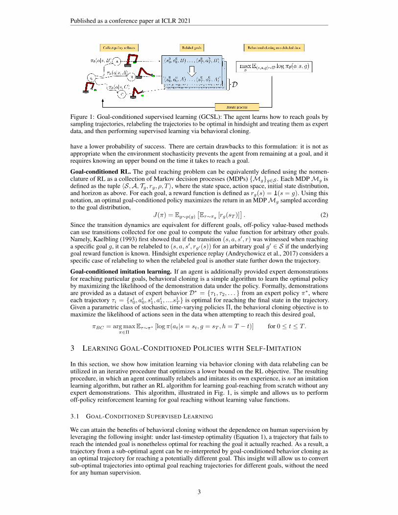
Figure 1: Goal-conditioned supervised learning (GCSL): The agent learns how to reach goals bysampling trajectories, relabeling the trajectories to be optimal in hindsight and treating them as expertdata, and then performing supervised learning via behavioral cloning.

have a lower probability of success. There are certain drawbacks to this formulation: it is not asappropriate when the environment stochasticity prevents the agent from remaining at a goal, and itrequires knowing an upper bound on the time it takes to reach a goal.

Goal-conditioned RL. The goal reaching problem can be equivalently defined using the nomen-clature of RL as a collection of Markov decision processes (MDPs) {Mg}g∈S . Each MDPMg isdefined as the tuple 〈S,A, Tg, rg, ρ, T 〉, where the state space, action space, initial state distribution,and horizon as above. For each goal, a reward function is defined as rg(s) = 1(s = g). Using thisnotation, an optimal goal-conditioned policy maximizes the return in an MDPMg sampled accordingto the goal distribution,

J(π) = Eg∼p(g)[Eτ∼πg [rg(sT )]

]. (2)

Since the transition dynamics are equivalent for different goals, off-policy value-based methodscan use transitions collected for one goal to compute the value function for arbitrary other goals.Namely, Kaelbling (1993) first showed that if the transition (s, a, s′, r) was witnessed when reachinga specific goal g, it can be relabeled to (s, a, s′, rg′(s)) for an arbitrary goal g′ ∈ S if the underlyinggoal reward function is known. Hindsight experience replay (Andrychowicz et al., 2017) considers aspecific case of relabeling to when the relabeled goal is another state further down the trajectory.

Goal-conditioned imitation learning. If an agent is additionally provided expert demonstrationsfor reaching particular goals, behavioral cloning is a simple algorithm to learn the optimal policyby maximizing the likelihood of the demonstration data under the policy. Formally, demonstrationsare provided as a dataset of expert behavior D∗ = {τ1, τ2, . . . } from an expert policy π∗, whereeach trajectory τi = {si0, ai0, si1, ai1, ....s1

T } is optimal for reaching the final state in the trajectory.Given a parametric class of stochastic, time-varying policies Π, the behavioral cloning objective is tomaximize the likelihood of actions seen in the data when attempting to reach this desired goal,

πBC = arg maxπ∈Π

Eτ∼π∗ [log π(at|s = st, g = sT , h = T − t)] for 0 ≤ t ≤ T .

3 LEARNING GOAL-CONDITIONED POLICIES WITH SELF-IMITATION

In this section, we show how imitation learning via behavior cloning with data relabeling can beutilized in an iterative procedure that optimizes a lower bound on the RL objective. The resultingprocedure, in which an agent continually relabels and imitates its own experience, is not an imitationlearning algorithm, but rather an RL algorithm for learning goal-reaching from scratch without anyexpert demonstrations. This algorithm, illustrated in Fig. 1, is simple and allows us to performoff-policy reinforcement learning for goal reaching without learning value functions.

3.1 GOAL-CONDITIONED SUPERVISED LEARNING

We can attain the benefits of behavioral cloning without the dependence on human supervision byleveraging the following insight: under last-timestep optimality (Equation 1), a trajectory that fails toreach the intended goal is nonetheless optimal for reaching the goal it actually reached. As a result, atrajectory from a sub-optimal agent can be re-interpreted by goal-conditioned behavior cloning asan optimal trajectory for reaching a potentially different goal. This insight will allow us to convertsub-optimal trajectories into optimal goal reaching trajectories for different goals, without the needfor any human supervision.

3


Algorithm 1 Goal-Conditioned Supervised Learning (GCSL)

1: Initialize policy π1(· | s, g, h)2: Initialize dataset D((s, a, g, h))3: for k = 1, 2, 3, . . . do4: Sample g ∼ p(g), collect data with πk(· | ·, g).5: Log trajectory τ = (s0, a0, s1, a1, . . . sT , aT )6: Add tuples Dτ to dataset D . see Eq. 37: πk+1 ← arg maxπθ ED [log πθ(a | s, g, h)]8: end for

More precisely, consider a trajectory τ = {s1, a1, s2, a2, . . . , sT , aT } obtained by commanding thepolicy πθ(a | s, g, h) to reach some goal g. For any time step t and horizon h, the action at in statest is likely to be a good action for reaching st+h in h time steps (even if it is not a good actionfor reaching the originally commanded goal g), and thus can be treated as expert supervision forπθ(· | st, st+h, h). To obtain a concrete algorithm, we can relabel all time steps and horizons in atrajectory to create an expert dataset according to

Dτ = {(st, at, g = st+h, h) : t, h > 0, t+ h ≤ T}, (3)

with states st, corresponding actions at, the corresponding goal set to future state st+h and matchinghorizon h. Because the relabeling procedure is valid for any horizon, we can use any valid combinationof (st, at, st+h, h) tuples as supervision, for a total of

(T2

)optimal datapoints of (s, a, g, h) from a

single trajectory. This idea is related to data-relabeling for estimating the value function (Kaelbling,1993; Andrychowicz et al., 2017; Rauber et al., 2017), but our work shows that data-relabelling canalso be used to re-interpret data from a sub-optimal agent as though the data came from an optimalagent (with a different goal).

We then use this relabeled dataset for goal-conditioned behavior cloning. Algorithm 1 summarizesthe approach: (1) Sample a goal from a target goal distribution p(g). (2) Execute the currentpolicy π(a|s, g, h) for T steps in the environment to collect a potentially suboptimal trajectory τ .(3) Relabel the trajectory (Equation. 3) to add

(T2

)new expert tuples (st, at, st+h, h) to the training

dataset. (4) Perform supervised learning on the entire dataset to update the policy π(a|s, g, h) viamaximum likelihood. We term this iterative procedure of sampling trajectories, relabeling them, andtraining a policy until convergence goal-conditioned supervised learning (GCSL). This algorithm canuse all of the prior off-policy data in the training dataset because this data continues to remain optimalunder the notion of goal-reaching optimality that was defined in Section 2, but does not require anyexplicit value function learning.Perhaps surprisingly, this procedure optimizes a lower bound on anRL objective, as we will show in Section 3.2.

The GCSL algorithm (as described above) can learn to reach goals from the target distribution p(g)simply using iterated behavioral cloning. This goal reaching algorithm is off-policy, optimizes asimple supervised learning objective, and is easy to implement and tune without the need for anyexplicit reward function engineering or demonstrations. Additionally, since GCSL uses a goal-conditioned imitation learning algorithm as a sub procedure, if demonstrations or off-policy data areavailable, it is easier to incorporate this data into training than with off-policy value function methods.

3.2 THEORETICAL ANALYSIS

We now formally analyze GCSL to verify that it solves the goal-reaching problem, quantify howerrors in approximation of the objective manifest in goal-reaching performance, and understand howit relates to existing RL algorithms. Specifically, we derive the algorithm as the optimization of alower bound of the true goal-reaching objective, and we show that under certain conditions on theenvironment, minimizing the GCSL objective enables performance guarantees on the learned policy.

We start by describing the objective function being optimized by GCSL. For ease of presentation, wemake the simplifying assumption that the trajectories are collected from a single policy πold, and thatrelabelling is only done with goals at the last timestep (g = sT ). GCSL performs goal-conditionedbehavioral cloning on a distribution of trajectories πold(τ) = Eg∼p(g)[πold(τ |g)], resulting in thefollowing objective:

4


JGCSL(π) = Eτ∼πold(τ)

[T∑t=0

log π(a = at|s = st, g = sT , h = T − t)

].

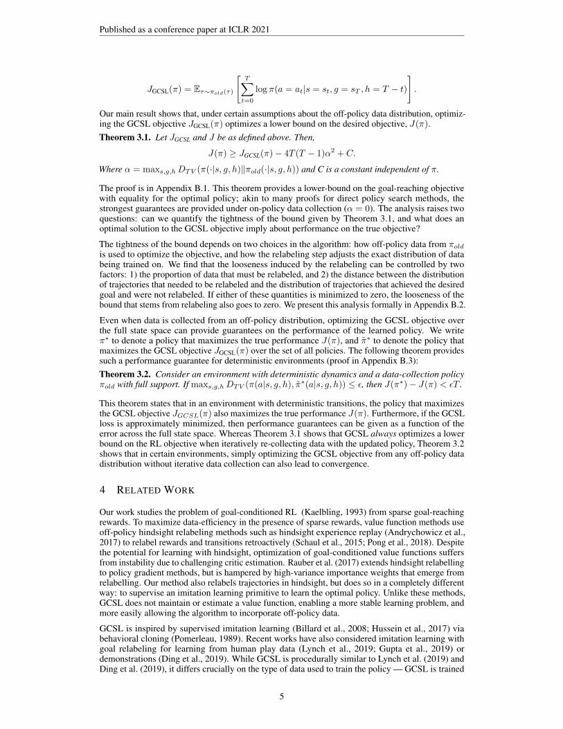
Our main result shows that, under certain assumptions about the off-policy data distribution, optimiz-ing the GCSL objective JGCSL(π) optimizes a lower bound on the desired objective, J(π).Theorem 3.1. Let JGCSL and J be as defined above. Then,

J(π) ≥ JGCSL(π)− 4T (T − 1)α2 + C.

Where α = maxs,g,hDTV (π(·|s, g, h)‖πold(·|s, g, h)) and C is a constant independent of π.

The proof is in Appendix B.1. This theorem provides a lower-bound on the goal-reaching objectivewith equality for the optimal policy; akin to many proofs for direct policy search methods, thestrongest guarantees are provided under on-policy data collection (α = 0). The analysis raises twoquestions: can we quantify the tightness of the bound given by Theorem 3.1, and what does anoptimal solution to the GCSL objective imply about performance on the true objective?

The tightness of the bound depends on two choices in the algorithm: how off-policy data from πoldis used to optimize the objective, and how the relabeling step adjusts the exact distribution of databeing trained on. We find that the looseness induced by the relabeling can be controlled by twofactors: 1) the proportion of data that must be relabeled, and 2) the distance between the distributionof trajectories that needed to be relabeled and the distribution of trajectories that achieved the desiredgoal and were not relabeled. If either of these quantities is minimized to zero, the looseness of thebound that stems from relabeling also goes to zero. We present this analysis formally in Appendix B.2.

Even when data is collected from an off-policy distribution, optimizing the GCSL objective overthe full state space can provide guarantees on the performance of the learned policy. We writeπ∗ to denote a policy that maximizes the true performance J(π), and π∗ to denote the policy thatmaximizes the GCSL objective JGCSL(π) over the set of all policies. The following theorem providessuch a performance guarantee for deterministic environments (proof in Appendix B.3):Theorem 3.2. Consider an environment with deterministic dynamics and a data-collection policyπold with full support. If maxs,g,hDTV (π(a|s, g, h), π∗(a|s, g, h)) ≤ ε, then J(π∗)− J(π) < εT .

This theorem states that in an environment with deterministic transitions, the policy that maximizesthe GCSL objective JGCSL(π) also maximizes the true performance J(π). Furthermore, if the GCSLloss is approximately minimized, then performance guarantees can be given as a function of theerror across the full state space. Whereas Theorem 3.1 shows that GCSL always optimizes a lowerbound on the RL objective when iteratively re-collecting data with the updated policy, Theorem 3.2shows that in certain environments, simply optimizing the GCSL objective from any off-policy datadistribution without iterative data collection can also lead to convergence.

4 RELATED WORK

Our work studies the problem of goal-conditioned RL (Kaelbling, 1993) from sparse goal-reachingrewards. To maximize data-efficiency in the presence of sparse rewards, value function methods useoff-policy hindsight relabeling methods such as hindsight experience replay (Andrychowicz et al.,2017) to relabel rewards and transitions retroactively (Schaul et al., 2015; Pong et al., 2018). Despitethe potential for learning with hindsight, optimization of goal-conditioned value functions suffersfrom instability due to challenging critic estimation. Rauber et al. (2017) extends hindsight relabellingto policy gradient methods, but is hampered by high-variance importance weights that emerge fromrelabelling. Our method also relabels trajectories in hindsight, but does so in a completely differentway: to supervise an imitation learning primitive to learn the optimal policy. Unlike these methods,GCSL does not maintain or estimate a value function, enabling a more stable learning problem, andmore easily allowing the algorithm to incorporate off-policy data.

GCSL is inspired by supervised imitation learning (Billard et al., 2008; Hussein et al., 2017) viabehavioral cloning (Pomerleau, 1989). Recent works have also considered imitation learning withgoal relabeling for learning from human play data (Lynch et al., 2019; Gupta et al., 2019) ordemonstrations (Ding et al., 2019). While GCSL is procedurally similar to Lynch et al. (2019) andDing et al. (2019), it differs crucially on the type of data used to train the policy — GCSL is trained

5


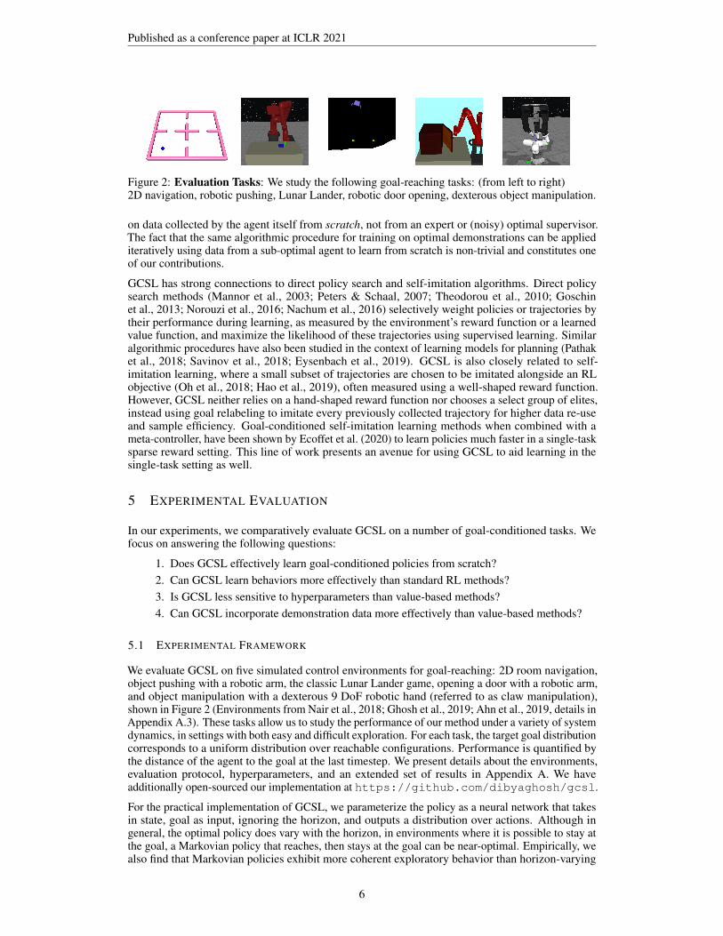
Figure 2: Evaluation Tasks: We study the following goal-reaching tasks: (from left to right)2D navigation, robotic pushing, Lunar Lander, robotic door opening, dexterous object manipulation.

on data collected by the agent itself from scratch, not from an expert or (noisy) optimal supervisor.The fact that the same algorithmic procedure for training on optimal demonstrations can be appliediteratively using data from a sub-optimal agent to learn from scratch is non-trivial and constitutes oneof our contributions.

GCSL has strong connections to direct policy search and self-imitation algorithms. Direct policysearch methods (Mannor et al., 2003; Peters & Schaal, 2007; Theodorou et al., 2010; Goschinet al., 2013; Norouzi et al., 2016; Nachum et al., 2016) selectively weight policies or trajectories bytheir performance during learning, as measured by the environment’s reward function or a learnedvalue function, and maximize the likelihood of these trajectories using supervised learning. Similaralgorithmic procedures have also been studied in the context of learning models for planning (Pathaket al., 2018; Savinov et al., 2018; Eysenbach et al., 2019). GCSL is also closely related to self-imitation learning, where a small subset of trajectories are chosen to be imitated alongside an RLobjective (Oh et al., 2018; Hao et al., 2019), often measured using a well-shaped reward function.However, GCSL neither relies on a hand-shaped reward function nor chooses a select group of elites,instead using goal relabeling to imitate every previously collected trajectory for higher data re-useand sample efficiency. Goal-conditioned self-imitation learning methods when combined with ameta-controller, have been shown by Ecoffet et al. (2020) to learn policies much faster in a single-tasksparse reward setting. This line of work presents an avenue for using GCSL to aid learning in thesingle-task setting as well.

5 EXPERIMENTAL EVALUATION

In our experiments, we comparatively evaluate GCSL on a number of goal-conditioned tasks. Wefocus on answering the following questions:

1. Does GCSL effectively learn goal-conditioned policies from scratch?2. Can GCSL learn behaviors more effectively than standard RL methods?3. Is GCSL less sensitive to hyperparameters than value-based methods?4. Can GCSL incorporate demonstration data more effectively than value-based methods?

5.1 EXPERIMENTAL FRAMEWORK

We evaluate GCSL on five simulated control environments for goal-reaching: 2D room navigation,object pushing with a robotic arm, the classic Lunar Lander game, opening a door with a robotic arm,and object manipulation with a dexterous 9 DoF robotic hand (referred to as claw manipulation),shown in Figure 2 (Environments from Nair et al., 2018; Ghosh et al., 2019; Ahn et al., 2019, details inAppendix A.3). These tasks allow us to study the performance of our method under a variety of systemdynamics, in settings with both easy and difficult exploration. For each task, the target goal distributioncorresponds to a uniform distribution over reachable configurations. Performance is quantified bythe distance of the agent to the goal at the last timestep. We present details about the environments,evaluation protocol, hyperparameters, and an extended set of results in Appendix A. We haveadditionally open-sourced our implementation at https://github.com/dibyaghosh/gcsl.

For the practical implementation of GCSL, we parameterize the policy as a neural network that takesin state, goal as input, ignoring the horizon, and outputs a distribution over actions. Although ingeneral, the optimal policy does vary with the horizon, in environments where it is possible to stay atthe goal, a Markovian policy that reaches, then stays at the goal can be near-optimal. Empirically, wealso find that Markovian policies exhibit more coherent exploratory behavior than horizon-varying

6

https://github.com/dibyaghosh/gcsl


0.0 0.5 1.0 1.5 2.01e5

0.25

0.50

Dis

tanc

e

Four Rooms

0.0 0.5 1.01e6

0.05

0.10

0.15

Sawyer Pushing

0.0 0.5 1.0 1.5 2.01e5

0

1

Lunar Lander

0.0 0.5 1.0Timesteps 1e6

0.0

0.2

0.4

Dis

tanc

e

Door Opening


0.5

1.0

1.5

Claw Manipulation

GCSLPPOTD3-HER

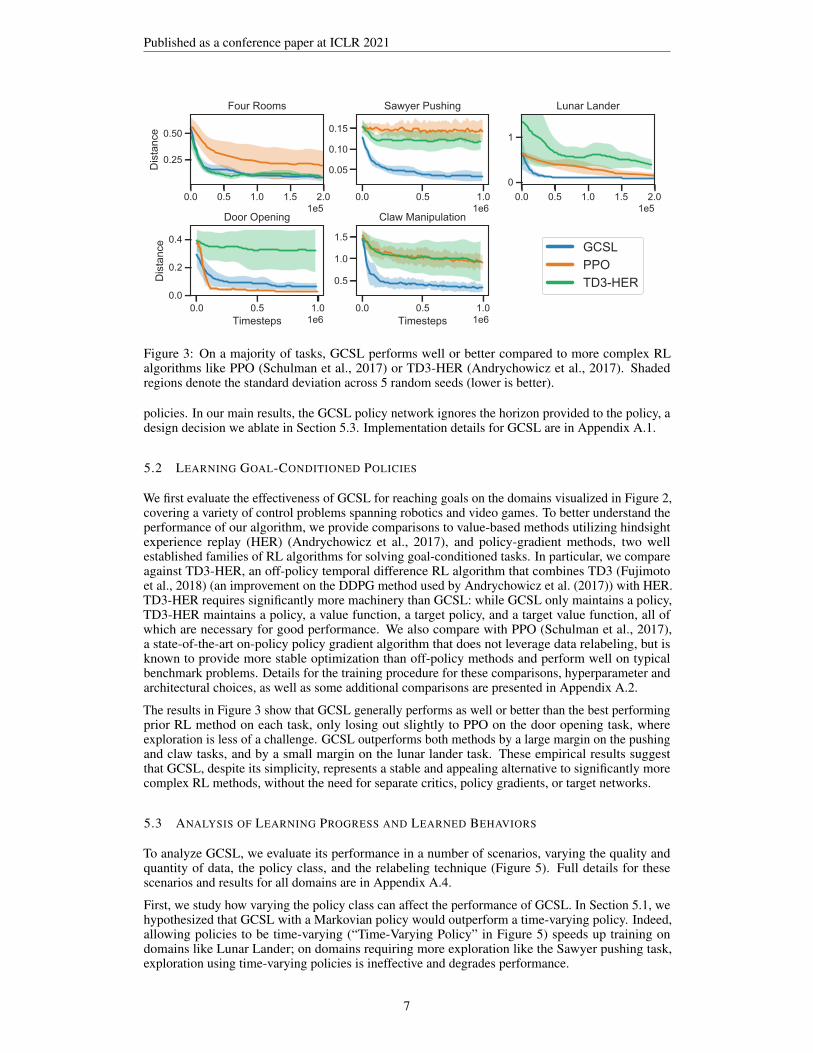
Figure 3: On a majority of tasks, GCSL performs well or better compared to more complex RLalgorithms like PPO (Schulman et al., 2017) or TD3-HER (Andrychowicz et al., 2017). Shadedregions denote the standard deviation across 5 random seeds (lower is better).

policies. In our main results, the GCSL policy network ignores the horizon provided to the policy, adesign decision we ablate in Section 5.3. Implementation details for GCSL are in Appendix A.1.

5.2 LEARNING GOAL-CONDITIONED POLICIES

We first evaluate the effectiveness of GCSL for reaching goals on the domains visualized in Figure 2,covering a variety of control problems spanning robotics and video games. To better understand theperformance of our algorithm, we provide comparisons to value-based methods utilizing hindsightexperience replay (HER) (Andrychowicz et al., 2017), and policy-gradient methods, two wellestablished families of RL algorithms for solving goal-conditioned tasks. In particular, we compareagainst TD3-HER, an off-policy temporal difference RL algorithm that combines TD3 (Fujimotoet al., 2018) (an improvement on the DDPG method used by Andrychowicz et al. (2017)) with HER.TD3-HER requires significantly more machinery than GCSL: while GCSL only maintains a policy,TD3-HER maintains a policy, a value function, a target policy, and a target value function, all ofwhich are necessary for good performance. We also compare with PPO (Schulman et al., 2017),a state-of-the-art on-policy policy gradient algorithm that does not leverage data relabeling, but isknown to provide more stable optimization than off-policy methods and perform well on typicalbenchmark problems. Details for the training procedure for these comparisons, hyperparameter andarchitectural choices, as well as some additional comparisons are presented in Appendix A.2.

The results in Figure 3 show that GCSL generally performs as well or better than the best performingprior RL method on each task, only losing out slightly to PPO on the door opening task, whereexploration is less of a challenge. GCSL outperforms both methods by a large margin on the pushingand claw tasks, and by a small margin on the lunar lander task. These empirical results suggestthat GCSL, despite its simplicity, represents a stable and appealing alternative to significantly morecomplex RL methods, without the need for separate critics, policy gradients, or target networks.

5.3 ANALYSIS OF LEARNING PROGRESS AND LEARNED BEHAVIORS

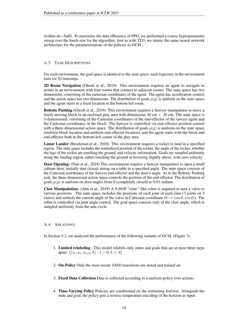
To analyze GCSL, we evaluate its performance in a number of scenarios, varying the quality andquantity of data, the policy class, and the relabeling technique (Figure 5). Full details for thesescenarios and results for all domains are in Appendix A.4.

First, we study how varying the policy class can affect the performance of GCSL. In Section 5.1, wehypothesized that GCSL with a Markovian policy would outperform a time-varying policy. Indeed,allowing policies to be time-varying (“Time-Varying Policy” in Figure 5) speeds up training ondomains like Lunar Lander; on domains requiring more exploration like the Sawyer pushing task,exploration using time-varying policies is ineffective and degrades performance.

7


Four Rooms Sawyer Pushing Claw Manipulation Lunar Lander Door Openingenv

0.0

0.5

1.0

Succ

ess

Rat

ioGCSLTD3

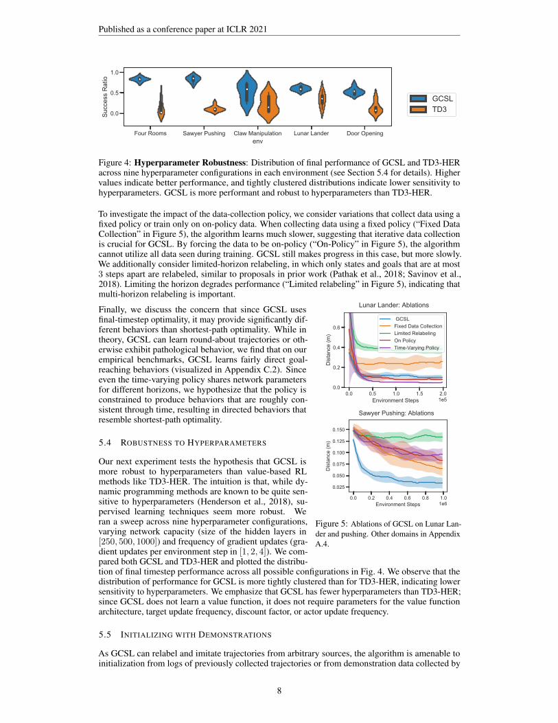
Figure 4: Hyperparameter Robustness: Distribution of final performance of GCSL and TD3-HERacross nine hyperparameter configurations in each environment (see Section 5.4 for details). Highervalues indicate better performance, and tightly clustered distributions indicate lower sensitivity tohyperparameters. GCSL is more performant and robust to hyperparameters than TD3-HER.

To investigate the impact of the data-collection policy, we consider variations that collect data using afixed policy or train only on on-policy data. When collecting data using a fixed policy (“Fixed DataCollection” in Figure 5), the algorithm learns much slower, suggesting that iterative data collectionis crucial for GCSL. By forcing the data to be on-policy (“On-Policy” in Figure 5), the algorithmcannot utilize all data seen during training. GCSL still makes progress in this case, but more slowly.We additionally consider limited-horizon relabeling, in which only states and goals that are at most3 steps apart are relabeled, similar to proposals in prior work (Pathak et al., 2018; Savinov et al.,2018). Limiting the horizon degrades performance (“Limited relabeling” in Figure 5), indicating thatmulti-horizon relabeling is important.

0.0 0.5 1.0 1.5 2.0Environment Steps 1e5

0.0

0.2

0.4

0.6D

ista

nce

(m)

GCSLFixed Data CollectionLimited RelabelingOn PolicyTime-Varying Policy

Lunar Lander: Ablations

0.0 0.2 0.4 0.6 0.8 1.0Environment Steps 1e6

0.025

0.050

0.075

0.100

0.125

0.150

Dis

tanc

e (m

)

Sawyer Pushing: Ablations

Figure 5: Ablations of GCSL on Lunar Lan-der and pushing. Other domains in AppendixA.4.

Finally, we discuss the concern that since GCSL usesfinal-timestep optimality, it may provide significantly dif-ferent behaviors than shortest-path optimality. While intheory, GCSL can learn round-about trajectories or oth-erwise exhibit pathological behavior, we find that on ourempirical benchmarks, GCSL learns fairly direct goal-reaching behaviors (visualized in Appendix C.2). Sinceeven the time-varying policy shares network parametersfor different horizons, we hypothesize that the policy isconstrained to produce behaviors that are roughly con-sistent through time, resulting in directed behaviors thatresemble shortest-path optimality.

5.4 ROBUSTNESS TO HYPERPARAMETERS

Our next experiment tests the hypothesis that GCSL ismore robust to hyperparameters than value-based RLmethods like TD3-HER. The intuition is that, while dy-namic programming methods are known to be quite sen-sitive to hyperparameters (Henderson et al., 2018), su-pervised learning techniques seem more robust. Weran a sweep across nine hyperparameter configurations,varying network capacity (size of the hidden layers in[250, 500, 1000]) and frequency of gradient updates (gra-dient updates per environment step in [1, 2, 4]). We com-pared both GCSL and TD3-HER and plotted the distribu-tion of final timestep performance across all possible configurations in Fig. 4. We observe that thedistribution of performance for GCSL is more tightly clustered than for TD3-HER, indicating lowersensitivity to hyperparameters. We emphasize that GCSL has fewer hyperparameters than TD3-HER;since GCSL does not learn a value function, it does not require parameters for the value functionarchitecture, target update frequency, discount factor, or actor update frequency.

5.5 INITIALIZING WITH DEMONSTRATIONS

As GCSL can relabel and imitate trajectories from arbitrary sources, the algorithm is amenable toinitialization from logs of previously collected trajectories or from demonstration data collected by

8


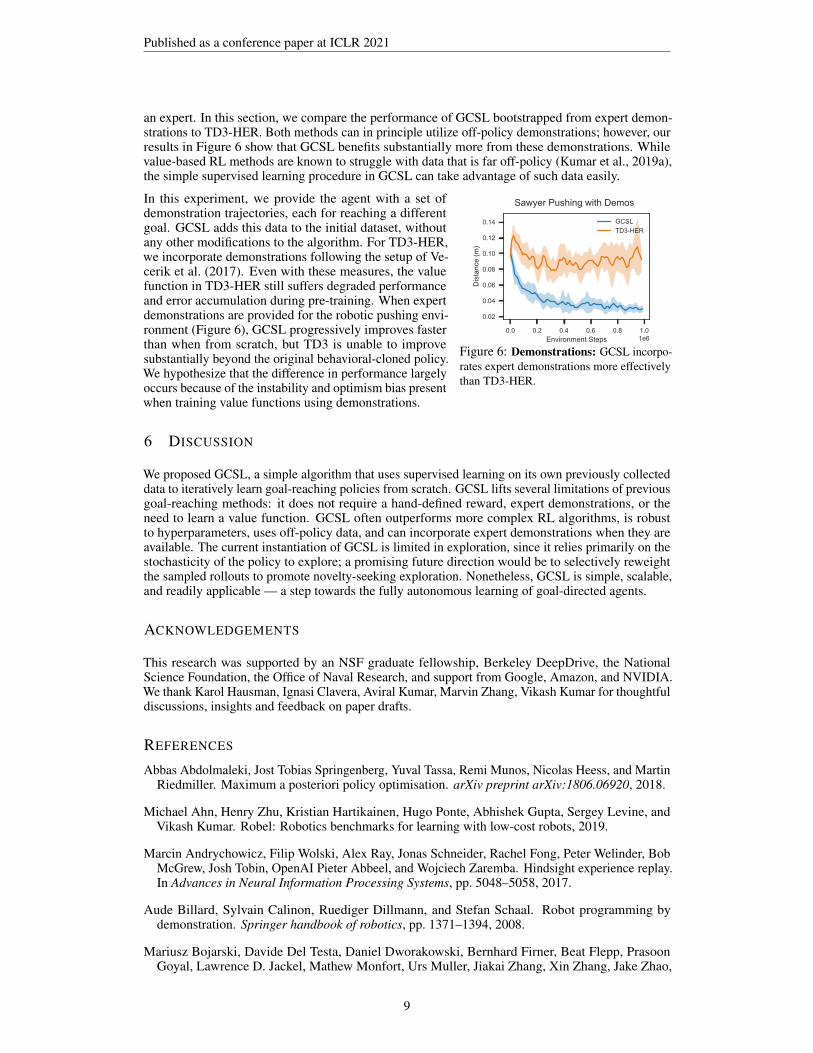
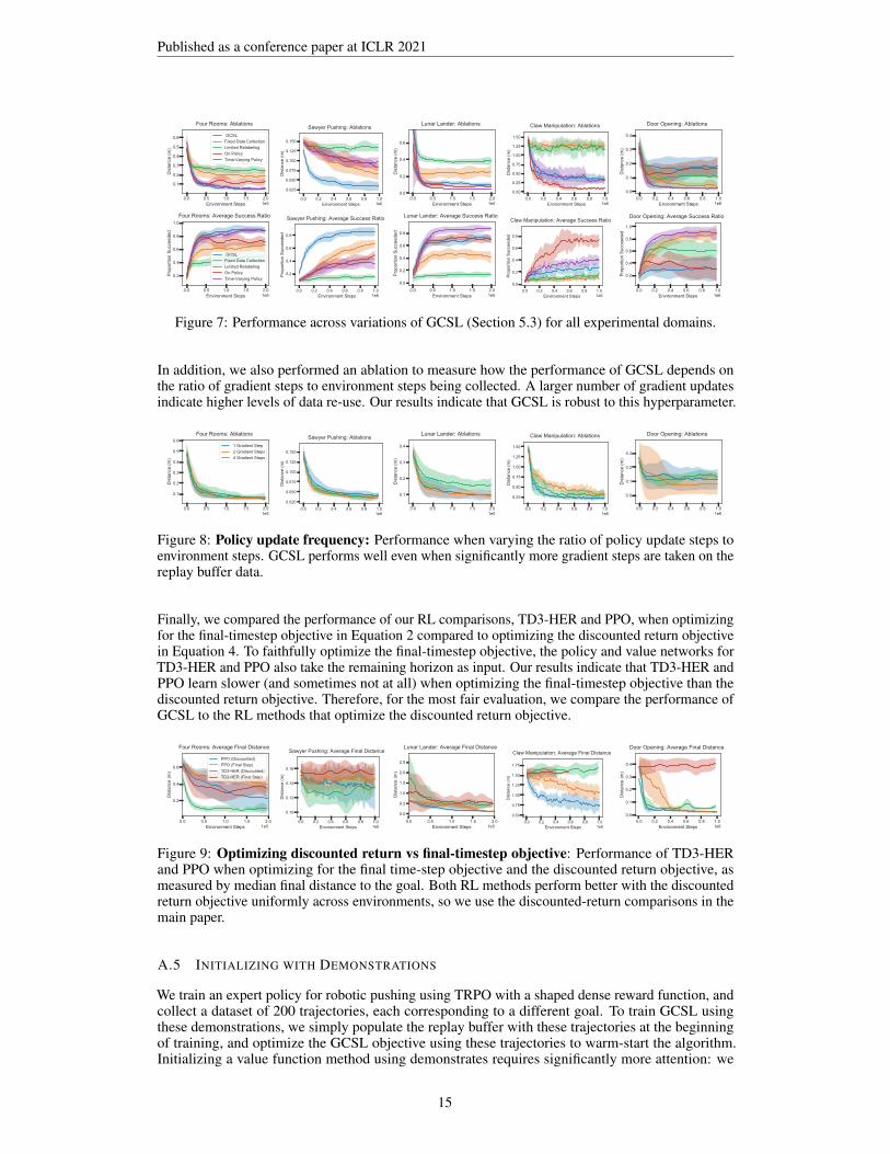
an expert. In this section, we compare the performance of GCSL bootstrapped from expert demon-strations to TD3-HER. Both methods can in principle utilize off-policy demonstrations; however, ourresults in Figure 6 show that GCSL benefits substantially more from these demonstrations. Whilevalue-based RL methods are known to struggle with data that is far off-policy (Kumar et al., 2019a),the simple supervised learning procedure in GCSL can take advantage of such data easily.


0.02

0.04

0.06

0.08

0.10

0.12

0.14

Dis

tanc

e (m

)

GCSLTD3-HER

Sawyer Pushing with Demos

Figure 6: Demonstrations: GCSL incorpo-rates expert demonstrations more effectivelythan TD3-HER.

In this experiment, we provide the agent with a set ofdemonstration trajectories, each for reaching a differentgoal. GCSL adds this data to the initial dataset, withoutany other modifications to the algorithm. For TD3-HER,we incorporate demonstrations following the setup of Ve-cerik et al. (2017). Even with these measures, the valuefunction in TD3-HER still suffers degraded performanceand error accumulation during pre-training. When expertdemonstrations are provided for the robotic pushing envi-ronment (Figure 6), GCSL progressively improves fasterthan when from scratch, but TD3 is unable to improvesubstantially beyond the original behavioral-cloned policy.We hypothesize that the difference in performance largelyoccurs because of the instability and optimism bias presentwhen training value functions using demonstrations.

6 DISCUSSION

We proposed GCSL, a simple algorithm that uses supervised learning on its own previously collecteddata to iteratively learn goal-reaching policies from scratch. GCSL lifts several limitations of previousgoal-reaching methods: it does not require a hand-defined reward, expert demonstrations, or theneed to learn a value function. GCSL often outperforms more complex RL algorithms, is robustto hyperparameters, uses off-policy data, and can incorporate expert demonstrations when they areavailable. The current instantiation of GCSL is limited in exploration, since it relies primarily on thestochasticity of the policy to explore; a promising future direction would be to selectively reweightthe sampled rollouts to promote novelty-seeking exploration. Nonetheless, GCSL is simple, scalable,and readily applicable — a step towards the fully autonomous learning of goal-directed agents.

ACKNOWLEDGEMENTS

This research was supported by an NSF graduate fellowship, Berkeley DeepDrive, the NationalScience Foundation, the Office of Naval Research, and support from Google, Amazon, and NVIDIA.We thank Karol Hausman, Ignasi Clavera, Aviral Kumar, Marvin Zhang, Vikash Kumar for thoughtfuldiscussions, insights and feedback on paper drafts.

REFERENCES

Abbas Abdolmaleki, Jost Tobias Springenberg, Yuval Tassa, Remi Munos, Nicolas Heess, and MartinRiedmiller. Maximum a posteriori policy optimisation. arXiv preprint arXiv:1806.06920, 2018.

Michael Ahn, Henry Zhu, Kristian Hartikainen, Hugo Ponte, Abhishek Gupta, Sergey Levine, andVikash Kumar. Robel: Robotics benchmarks for learning with low-cost robots, 2019.

Marcin Andrychowicz, Filip Wolski, Alex Ray, Jonas Schneider, Rachel Fong, Peter Welinder, BobMcGrew, Josh Tobin, OpenAI Pieter Abbeel, and Wojciech Zaremba. Hindsight experience replay.In Advances in Neural Information Processing Systems, pp. 5048–5058, 2017.

Aude Billard, Sylvain Calinon, Ruediger Dillmann, and Stefan Schaal. Robot programming bydemonstration. Springer handbook of robotics, pp. 1371–1394, 2008.

Mariusz Bojarski, Davide Del Testa, Daniel Dworakowski, Bernhard Firner, Beat Flepp, PrasoonGoyal, Lawrence D. Jackel, Mathew Monfort, Urs Muller, Jiakai Zhang, Xin Zhang, Jake Zhao,

9


and Karol Zieba. End to end learning for self-driving cars. CoRR, abs/1604.07316, 2016. URLhttp://arxiv.org/abs/1604.07316.

Greg Brockman, Vicki Cheung, Ludwig Pettersson, Jonas Schneider, John Schulman, Jie Tang, andWojciech Zaremba. Openai gym. CoRR, abs/1606.01540, 2016. URL http://arxiv.org/abs/1606.01540.

Yiming Ding, Carlos Florensa, Mariano Phielipp, and Pieter Abbeel. Goal conditioned imitationlearning. In Advances in Neural Information Processing Systems, 2019.

Adrien Ecoffet, Joost Huizinga, Joel Lehman, Kenneth O. Stanley, and Jeff Clune. First return thenexplore, 2020.

Benjamin Eysenbach, Ruslan Salakhutdinov, and Sergey Levine. Search on the replay buffer:Bridging planning and reinforcement learning. arXiv preprint arXiv:1906.05253, 2019.

Scott Fujimoto, David Meger, and Doina Precup. Off-policy deep reinforcement learning withoutexploration. arXiv preprint arXiv:1812.02900, 2018.

Dibya Ghosh, Abhishek Gupta, and Sergey Levine. Learning actionable representations with goalconditioned policies. In International Conference on Learning Representations, 2019.

Sergiu Goschin, Ari Weinstein, and Michael Littman. The cross-entropy method optimizes forquantiles. In International Conference on Machine Learning, pp. 1193–1201, 2013.

Abhishek Gupta, Vikash Kumar, Corey Lynch, Sergey Levine, and Karol Hausman. Relay policy learn-ing: Solving long-horizon tasks via imitation and reinforcement learning. CoRR, abs/1910.11956,2019. URL http://arxiv.org/abs/1910.11956.

Xiaotian Hao, Weixun Wang, Jianye Hao, and Y. Yang. Independent generative adversarial self-imitation learning in cooperative multiagent systems. In AAMAS, 2019.

Peter Henderson, Riashat Islam, Philip Bachman, Joelle Pineau, Doina Precup, and David Meger.Deep reinforcement learning that matters. In Thirty-Second AAAI Conference on Artificial Intelli-gence, 2018.

Ahmed Hussein, Mohamed Medhat Gaber, Eyad Elyan, and Chrisina Jayne. Imitation learning: Asurvey of learning methods. ACM Computing Surveys (CSUR), 50(2):21, 2017.

Leslie Pack Kaelbling. Learning to achieve goals. In International Joint Conference on ArtificialIntelligence (IJCAI), pp. 1094–1098, 1993.

Sham Kakade and John Langford. Approximately optimal approximate reinforcement learning. InProceedings of the Nineteenth International Conference on Machine Learning, ICML ’02, pp.267–274, San Francisco, CA, USA, 2002. Morgan Kaufmann Publishers Inc. ISBN 1-55860-873-7.URL http://dl.acm.org/citation.cfm?id=645531.656005.

Aviral Kumar, Justin Fu, George Tucker, and Sergey Levine. Stabilizing off-policy q-learning viabootstrapping error reduction. CoRR, abs/1906.00949, 2019a.

Aviral Kumar, Justin Fu, George Tucker, and Sergey Levine. Stabilizing off-policy q-learning viabootstrapping error reduction. arXiv preprint arXiv:1906.00949, 2019b.

Corey Lynch, Mohi Khansari, Ted Xiao, Vikash Kumar, Jonathan Tompson, Sergey Levine, andPierre Sermanet. Learning latent plans from play. arXiv preprint arXiv:1903.01973, 2019.

Shie Mannor, Reuven Y Rubinstein, and Yohai Gat. The cross entropy method for fast policysearch. In Proceedings of the 20th International Conference on Machine Learning (ICML-03), pp.512–519, 2003.

Ofir Nachum, Mohammad Norouzi, and Dale Schuurmans. Improving policy gradient by exploringunder-appreciated rewards. arXiv preprint arXiv:1611.09321, 2016.

10

http://arxiv.org/abs/1604.07316




http://dl.acm.org/citation.cfm?id=645531.656005


Ashvin V Nair, Vitchyr Pong, Murtaza Dalal, Shikhar Bahl, Steven Lin, and Sergey Levine. Visualreinforcement learning with imagined goals. In Advances in Neural Information ProcessingSystems, pp. 9191–9200, 2018.

Gerhard Neumann and Jan R Peters. Fitted q-iteration by advantage weighted regression. In Advancesin neural information processing systems, pp. 1177–1184, 2009.

Mohammad Norouzi, Samy Bengio, Navdeep Jaitly, Mike Schuster, Yonghui Wu, Dale Schuurmans,et al. Reward augmented maximum likelihood for neural structured prediction. In Advances InNeural Information Processing Systems, pp. 1723–1731, 2016.

Junhyuk Oh, Yijie Guo, Satinder Singh, and Honglak Lee. Self-imitation learning. In InternationalConference on Machine Learning, pp. 3875–3884, 2018.

Deepak Pathak, Parsa Mahmoudieh, Guanghao Luo, Pulkit Agrawal, Dian Chen, Yide Shentu, EvanShelhamer, Jitendra Malik, Alexei A Efros, and Trevor Darrell. Zero-shot visual imitation. InProceedings of the IEEE Conference on Computer Vision and Pattern Recognition Workshops, pp.2050–2053, 2018.

Xue Bin Peng, Aviral Kumar, Grace Zhang, and Sergey Levine. Advantage-weighted regression:Simple and scalable off-policy reinforcement learning. arXiv preprint arXiv:1910.00177, 2019.

Jan Peters and Stefan Schaal. Reinforcement learning by reward-weighted regression for operationalspace control. In Proceedings of the 24th international conference on Machine learning, pp.745–750. ACM, 2007.

Dean A Pomerleau. Alvinn: An autonomous land vehicle in a neural network. In Advances in neuralinformation processing systems, pp. 305–313, 1989.

Vitchyr Pong, Shixiang Gu, Murtaza Dalal, and Sergey Levine. Temporal difference models: Model-free deep rl for model-based control. arXiv preprint arXiv:1802.09081, 2018.

Paulo Rauber, Avinash Ummadisingu, Filipe Mutz, and Juergen Schmidhuber. Hindsight policygradients. arXiv preprint arXiv:1711.06006, 2017.

Stephane Ross, Geoffrey Gordon, and Drew Bagnell. A reduction of imitation learning and structuredprediction to no-regret online learning. In Geoffrey Gordon, David Dunson, and Miroslav Dudık(eds.), Proceedings of the Fourteenth International Conference on Artificial Intelligence and Statis-tics, volume 15 of Proceedings of Machine Learning Research, pp. 627–635, Fort Lauderdale, FL,USA, 11–13 Apr 2011. PMLR. URL http://proceedings.mlr.press/v15/ross11a.html.

Nikolay Savinov, Alexey Dosovitskiy, and Vladlen Koltun. Semi-parametric topological memory fornavigation. arXiv preprint arXiv:1803.00653, 2018.

Tom Schaul, Daniel Horgan, Karol Gregor, and David Silver. Universal value function approximators.In International conference on machine learning, pp. 1312–1320, 2015.

John Schulman, Sergey Levine, Pieter Abbeel, Michael Jordan, and Philipp Moritz. Trust regionpolicy optimization. In Francis Bach and David Blei (eds.), Proceedings of the 32nd InternationalConference on Machine Learning, volume 37 of Proceedings of Machine Learning Research, pp.1889–1897, Lille, France, 07–09 Jul 2015. PMLR.

John Schulman, Filip Wolski, Prafulla Dhariwal, Alec Radford, and Oleg Klimov. Proximal policyoptimization algorithms. CoRR, abs/1707.06347, 2017.

Evangelos Theodorou, Jonas Buchli, and Stefan Schaal. A generalized path integral control approachto reinforcement learning. journal of machine learning research, 11(Nov):3137–3181, 2010.

John N Tsitsiklis and Benjamin Van Roy. Analysis of temporal-diffference learning with functionapproximation. In Advances in neural information processing systems, pp. 1075–1081, 1997.

Hado van Hasselt, Yotam Doron, Florian Strub, Matteo Hessel, Nicolas Sonnerat, and Joseph Modayil.Deep reinforcement learning and the deadly triad. ArXiv, abs/1812.02648, 2018.

11

http://proceedings.mlr.press/v15/ross11a.html

http://proceedings.mlr.press/v15/ross11a.html


Mel Vecerik, Todd Hester, Jonathan Scholz, Fumin Wang, Olivier Pietquin, Bilal Piot, Nicolas Heess,Thomas Rothorl, Thomas Lampe, and Martin Riedmiller. Leveraging demonstrations for deepreinforcement learning on robotics problems with sparse rewards. arXiv preprint arXiv:1707.08817,2017.

12


A EXPERIMENTAL DETAILS

A.1 GOAL-CONDITIONED SUPERVISED LEARNING (GCSL)

GCSL iteratively performs maximum likelihood estimation using a dataset of relabeled trajectoriesthat have been previously collected by the agent. Here we present details about the policy class, datacollection procedure, and other design choices.

We parameterize a time-invariant policy using a neural network which takes as input state and goal(not the horizon), and returns probabilities for a discretized grid of actions of the action space. Theneural network concatenates the state and goal together, and passes the concatenated input into afeedforward network with two hidden layers of size 400 and 300 respectively, outputting logits foreach discretized action. Empirically, we have found GCSL to perform much better with larger choicesof neural networks; however, we use this two-layer neural network for fair comparisons to TD3-HER.The GCSL loss is optimized using the Adam optimizer with learning rate α = 5× 10−4, with a batchsize of 256, taking one gradient step for every step in the environment.

When executing in the environment, the first 10000 environment steps are taken according touniform random action selection, after which the data-collection policy is the greedy policy:a = arg maxa π(a|s, g). The replay buffer stores trajectories and relabels on the fly, with thesize of the buffer subject only to memory constraints. To clarify, instead of explicitly relabeling andstoring all

(T2

)possible tuples from a trajectory, we instead save the trajectory and relabel at training

time. When sampling from the dataset, a trajectory is chosen at random, a start index t and goalindex t′ > t are sampled uniformly at random, and the tuple corresponding to this state and goal arerelabelled and sampled.

A.2 RL COMPARISONS

We provide comparisons to two goal-reaching RL methods: TD3-HER and PPO. While GCSL is ableto efficiently optimize the last-timestep objective, RL methods that learn value functions performpoorly when optimizing this objective. We include results of RL methods optimizing the last-timestepobjective for completeness in Figure 9, but our main RL comparisons instead optimize the classicaldiscounted sum of returns:

J(π) = Eg∼p(g)[Eτ∼πg [∑t≤T

γtrg(st)]], (4)

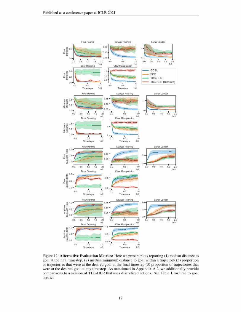
where reaching the goal leads to termination, the reward function remains the same, rg(s) = 1(s = g)and we use γ = 0.99. We log other metrics for these algorithms in Figure 12, and have included avariety of possible metrics.

TD3-HER (Fujimoto et al., 2018; Andrychowicz et al., 2017): To efficiently learn a value func-tion, we use hindsight relabelling. Specifically, a transition ((s, g), a, (s′, g)) gets relabeled to((s, g′), a, (s′, g′)), where g′ = g with probability 0.1, g′ = s′ with probability 0.5, and g′ = stfor some future state in the trajectory st with probability 0.4. As described in Section 2, the agentreceives a reward of 1 and the trajectory ends if the transition is relabeled to g′ = s′, and 0 otherwise.Under this formalism, the optimal value function, V ∗(s, g) ∝ γT (s,g), where T (s, g) is the minimumexpected time to go from s to g. Both the Q-function and the actor for TD3 are parametrized as neuralnetworks, with the same architecture (except final layers) for state-based domains as those for GCSL.We found the default values of learning rate, target update period, and number of critic updates to bethe best amongst our hyperparameter search across the domains (single set of hyperparameters for alldomains). Since GCSL uses discretized actions, we additionally compared to a version of TD3-HERthat also uses discretized actions (results in Figure 12). The performance of TD3-HER w/ discretizedactions decreases performance on the Claw task, increases on the Door Opening task, and has thesame performance on the other three environments.

PPO (Schulman et al., 2017): Because PPO is an on-policy RL algorithm, we cannot relabel goals,unlike in GCSL or TD3-HER. Instead, we provide a surrogate ε-ball indicator reward function:r(s, g) = 1(d(s, g) < ε), where ε is chosen appropriately for each environment. We emphasize thatthis reward function makes the policy optimization problem for PPO much easier, since while theother two methods only can check if two states are exactly equal, PPO also has access to the distance

13


(within an ε-ball). To maximize the data efficiency of PPO, we performed a coarse hyperparametersweep over the batch size for the algorithm. Just as with TD3, we mimic the same neural networkarchitecture for the parametrizations of the policies as GCSL.

A.3 TASK DESCRIPTIONS

For each environment, the goal space is identical to the state space; each trajectory in the environmentlasts for 50 timesteps.

2D Room Navigation (Ghosh et al., 2019) This environment requires an agent to navigate topoints in an environment with four rooms that connect to adjacent rooms. The state space has twodimensions, consisting of the cartesian coordinates of the agent. The agent has acceleration control,and the action space has two dimensions. The distribution of goals p(g) is uniform on the state space,and the agent starts in a fixed location in the bottom left room.

Robotic Pushing (Ghosh et al., 2019) This environment requires a Sawyer manipulator to move afreely moving block in an enclosed play area with dimensions 40 cm × 20 cm. The state space is4-dimensional, consisting of the Cartesian coordinates of the end-effector of the sawyer agent andthe Cartesian coordinates of the block. The Sawyer is controlled via end-effector position controlwith a three-dimensional action space. The distribution of goals p(g) is uniform on the state space(uniform block location and uniform end-effector location), and the agent starts with the block andend-effector both in the bottom-left corner of the play area.

Lunar Lander (Brockman et al., 2016) This environment requires a rocket to land in a specifiedregion. The state space includes the normalized position of the rocket, the angle of the rocket, whetherthe legs of the rocket are touching the ground, and velocity information. Goals are sampled uniformlyalong the landing region, either touching the ground or hovering slightly above, with zero velocity.

Door Opening: (Nair et al., 2018) This environment requires a Sawyer manipulator to open a smallcabinet door, initially shut closed, sitting on a table to a specified angle. The state space consists ofthe Cartesian coordinates of the Sawyer end-effector and the door’s angle. As in the Robotic Pushingtask, the three-dimensional action space controls the position of the end-effector. The distribution ofgoals p(g) is uniform on door angles from 0 (completely closed) to 0.83 radians.

Claw Manipulation: (Ahn et al., 2019) A 9-DOF ”claw”-like robot is required to turn a valve tovarious positions . The state space includes the positions of each joint of each claw (3 joints on 3claws) and embeds the current angle of the valve in Cartesian coordinate (θ 7→ (sin θ, cos θ)). Therobot is controlled via joint angle control. The goal space consists only of the claw angle, which issampled uniformly from the unit circle.

A.4 ABLATIONS

In Section 5.3, we analyzed the performance of the following variants of GCSL (Figure 7).

1. Limited relabeling - This model relabels only states and goals that are at most three stepsapart: {(st, at, st+h, h) : t > 0, h ≤ 3}

2. On-Policy Only the most recent 10000 transitions are stored and trained on.

3. Fixed Data Collection Data is collected according to a uniform policy over actions.

4. Time-Varying Policy Policies are conditioned on the remaining horizon. Alongside thestate and goal, the policy gets a reverse temperature encoding of the horizon as input.

14



0.1

0.2

0.3

0.4

0.5

0.6

Dis

tanc

e (m

)


Four Rooms: Ablations


0.025

0.050

0.075

0.100

0.125

0.150

Dis

tanc

e (m

)



0.0

0.2

0.4

0.6

Dis

tanc

e (m

)



0.00

0.25

0.50

0.75

1.00

1.25

1.50

Dis

tanc

e (m

)

Claw Manipulation: Ablations


0.0

0.1

0.2

0.3

0.4

Dis

tanc

e (m

)

Door Opening: Ablations


0.2

0.4

0.6

0.8

1.0

Prop

ortio

n Su

ccee

ded


Four Rooms: Average Success Ratio


0.2

0.4

0.6

0.8

Prop

ortio

n Su

ccee

ded

Sawyer Pushing: Average Success Ratio


0.0

0.2

0.4

0.6

0.8

Prop

ortio

n Su

ccee

ded

Lunar Lander: Average Success Ratio


0.0

0.2

0.4

0.6

0.8

Prop

ortio

n Su

ccee

ded

Claw Manipulation: Average Success Ratio


0.2

0.4

0.6

0.8

1.0

Prop

ortio

n Su

ccee

ded

Door Opening: Average Success Ratio

Figure 7: Performance across variations of GCSL (Section 5.3) for all experimental domains.

In addition, we also performed an ablation to measure how the performance of GCSL depends onthe ratio of gradient steps to environment steps being collected. A larger number of gradient updatesindicate higher levels of data re-use. Our results indicate that GCSL is robust to this hyperparameter.

0.0 0.5 1.0 1.5 2.01e5

0.1

0.2

0.3

0.4

0.5

0.6

Dis

tanc

e (m

)

1 Gradient Step2 Gradient Steps4 Gradient Steps

Four Rooms: Ablations

0.0 0.2 0.4 0.6 0.8 1.01e6

0.025

0.050

0.075

0.100

0.125

0.150

Dis

tanc

e (m

)


0.0 0.5 1.0 1.5 2.01e5

0.1

0.2

0.3

0.4

Dis

tanc

e (m

)


0.0 0.2 0.4 0.6 0.8 1.01e6

0.25

0.50

0.75

1.00

1.25

1.50

Dis

tanc

e (m

)

Claw Manipulation: Ablations

0.0 0.2 0.4 0.6 0.8 1.01e6

0.0

0.1

0.2

0.3

Dis

tanc

e (m

)

Door Opening: Ablations

Figure 8: Policy update frequency: Performance when varying the ratio of policy update steps toenvironment steps. GCSL performs well even when significantly more gradient steps are taken on thereplay buffer data.

Finally, we compared the performance of our RL comparisons, TD3-HER and PPO, when optimizingfor the final-timestep objective in Equation 2 compared to optimizing the discounted return objectivein Equation 4. To faithfully optimize the final-timestep objective, the policy and value networks forTD3-HER and PPO also take the remaining horizon as input. Our results indicate that TD3-HER andPPO learn slower (and sometimes not at all) when optimizing the final-timestep objective than thediscounted return objective. Therefore, for the most fair evaluation, we compare the performance ofGCSL to the RL methods that optimize the discounted return objective.


0.2

0.4

0.6

Dis

tanc

e (m

)

PPO (Discounted)PPO (Final Step)TD3-HER (Discounted)TD3-HER (Final Step)

Four Rooms: Average Final Distance


0.10

0.12

0.14

0.16

Dis

tanc

e (m

)

Sawyer Pushing: Average Final Distance


0.0

0.5

1.0

1.5

2.0

2.5

Dis

tanc

e (m

)

Lunar Lander: Average Final Distance


0.50

0.75

1.00

1.25

1.50

1.75

Dis

tanc

e (m

)

Claw Manipulation: Average Final Distance


0.0

0.1

0.2

0.3

0.4

Dis

tanc

e (m

)

Door Opening: Average Final Distance

Figure 9: Optimizing discounted return vs final-timestep objective: Performance of TD3-HERand PPO when optimizing for the final time-step objective and the discounted return objective, asmeasured by median final distance to the goal. Both RL methods perform better with the discountedreturn objective uniformly across environments, so we use the discounted-return comparisons in themain paper.

A.5 INITIALIZING WITH DEMONSTRATIONS

We train an expert policy for robotic pushing using TRPO with a shaped dense reward function, andcollect a dataset of 200 trajectories, each corresponding to a different goal. To train GCSL usingthese demonstrations, we simply populate the replay buffer with these trajectories at the beginningof training, and optimize the GCSL objective using these trajectories to warm-start the algorithm.Initializing a value function method using demonstrates requires significantly more attention: we

15


perform the following procedure. First, we perform goal-conditioned behavior cloning to learn aninitial policy πBC . Next, we collect 200 new trajectories in the environment using a uniform datacollection scheme. Using this dataset of 400 trajectories, we perform policy evaluation on πBCto learn QπBC using policy evaluation via bootstrapping. Having trained such an estimate of theQ-function, we initialize the policy and Q-function to these estimates, and run the appropriate valuefunction RL algorithm.

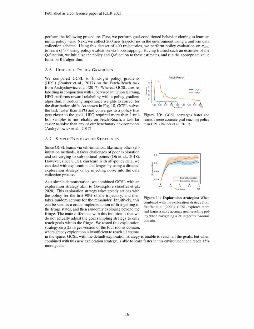
A.6 HINDSIGHT POLICY GRADIENTS

0.00 0.25 0.50 0.75 1.00 1.25 1.50 1.75 2.00Timesteps 1e6

0.1

0.2

0.3

0.4

0.5

Dis

tanc

e

GCSLHPG

Fetch Reach

Figure 10: GCSL converges faster andlearns a more accurate goal-reaching policythan HPG (Rauber et al., 2017)

We compared GCSL to hindsight policy gradients(HPG) (Rauber et al., 2017) on the Fetch-Reach taskfrom Andrychowicz et al. (2017). Whereas GCSL uses re-labelling in conjunction with supervised imitation learning,HPG performs reward relabeling with a policy gradientalgorithm, introducing importance weights to correct forthe distribution shift. As shown in Fig. 10, GCSL solvesthe task faster than HPG and converges to a policy thatgets closer to the goal. HPG required more than 1 mil-lion samples to run reliably on Fetch-Reach, a task fareasier to solve than any of our benchmark environments(Andrychowicz et al., 2017)

A.7 SIMPLE EXPLORATION STRATEGIES

0.0 0.5 1.0 1.5 2.0Timesteps 1e5

0.2

0.4

0.6

0.8Su

cces

s R

ate

Default ExplorationExploration Strategy

Figure 11: Exploration strategies: Whencombined with the exploration strategy fromEcoffet et al. (2020), GCSL explores moreand learns a more accurate goal-reaching pol-icy when navigating a 2x larger four-roomsdomain.

Since GCSL learns via self-imitation, like many other self-imitation methods, it faces challenges of poor explorationand converging to sub-optimal points (Oh et al., 2018).However, since GCSL can learn with off-policy data, wecan deal with exploration challenges by using a directedexploration strategy or by injecting noise into the datacollection process.

As a simple demonstration, we combined GCSL with anexploration strategy akin to Go-Explore (Ecoffet et al.,2020). This exploration strategy takes greedy actions withthe policy for the first 90% of the trajectory, and thentakes random actions for the remainder. Intuitively, thiscan be seen as a crude implementation of first getting tothe fringe states, and then randomly exploring beyond thefringe. The main difference with this intuition is that wedo not actually adjust the goal sampling strategy to onlyreach goals within the fringe. We tested this explorationstrategy on a 2x larger version of the four rooms domain,where greedy exploration is insufficient to reach all regionsin the space. GCSL with the default exploration strategy is unable to reach all the goals, but whencombined with this new exploration strategy, is able to learn faster in this environment and reach 15%more goals.

16


0.0 0.5 1.0 1.5 2.01e5

0.0

0.5

Fina

lD

ista

nce

Four Rooms

0.0 0.5 1.01e6

0.05

0.10

0.15

Sawyer Pushing

0.0 0.5 1.0 1.5 2.01e5

0

1

Lunar Lander


0.0

0.2

0.4

Fina

lD

ista

nce

Door Opening


0.5

1.0

1.5

Claw Manipulation

GCSLPPOTD3-HERTD3-HER (Discrete)

0.0 0.5 1.0 1.5 2.01e5

0.0

0.2

0.4

Min

imum

Dis

tanc

e

Four Rooms

0.0 0.5 1.01e6

0.05

0.10

0.15

Sawyer Pushing

0.0 0.5 1.0 1.5 2.01e5

0

1

Lunar Lander


0.0

0.2

0.4

Min

imum

Dis

tanc

e

Door Opening


0

1

Claw Manipulation

0.0 0.5 1.0 1.5 2.01e5

0.0

0.5

1.0

Fina

lSu

cces

s R

ate

Four Rooms

0.0 0.5 1.01e6

0.25

0.50

Sawyer Pushing

0.0 0.5 1.0 1.5 2.01e5

0.0

0.5

Lunar Lander


0.0

0.5

1.0

Fina

lSu

cces

s R

ate

Door Opening


0.0

0.5

Claw Manipulation

0.0 0.5 1.0 1.5 2.01e5

0.0

0.5

1.0

Anyt

ime

Succ

ess

Rat

e

Four Rooms

0.0 0.5 1.01e6

0.25

0.50

0.75Sawyer Pushing

0.0 0.5 1.0 1.5 2.01e5

0.0

0.5

1.0Lunar Lander


0.0

0.5

1.0

Anyt

ime

Succ

ess

Rat

e

Door Opening


0.0

0.5

1.0Claw Manipulation

Figure 12: Alternative Evaluation Metrics: Here we present plots reporting (1) median distance togoal at the final timestep, (2) median minimum distance to goal within a trajectory (3) proportionof trajectories that were at the desired goal at the final timestep (3) proportion of trajectories thatwere at the desired goal at any timestep. As mentioned in Appendix A.2, we additionally providecomparisons to a version of TD3-HER that uses discretized actions. See Table 1 for time to goalmetrics

17


B THEORETICAL ANALYSIS

B.1 PROOF OF THEOREM 4.1

We will assume a discrete state space in this proof, and denote a trajectory as τ ={s0, a0, . . . , sT , aT }. Let the notation G(τ) = sT denote the final state of a trajectory, whichrepresents the goal that the trajectory reached. As there can be multiple paths to a goal, we letτg = {τ : G(τ) = g} denote the set of trajectories that reach a particular goal g. We abbreviate apolicy’s trajectory distribution as π(τ |g) = p(s0)

∏Tt=0 π(at|st, g)T (st+1|st, at). The target goal-

reaching objective we wish to optimize is the probability of reaching a commanded goal, when goalsare sampled from a pre-specified distribution p(g).

J(π) = Eg∼p(g),τ∼π(τ |g)[1[G(τ) = g]]

GCSL optimizes the following objective, where the log-likelihood of the actions conditioned onthe goals actually reached by the policy, G(τ). The distribution of trajectories used to optimize theobjective is collected through a different policy, πold. We write πold(τ) = Eg∼p(g)[πold(τ |g)] toconcisely represent the marginalized distribution of trajectories from πold.

JGCSL(π) = Eτ∼πold(τ)

[T∑t=0

log π(at|st,G(τ))

]To analyze how this objective relates to J(π), we first analyze the relationship between J(π) and asurrogate objective, given by

Jsurr(π) = Eg∼p(g),τ∼πold(τ |g) [1[G(τ) = g] log π(τ |g)]

Theorem 1 from Schulman et al. (2015) states that

J(π) ≥ Jsurr(π)− 4γε

(1− γ)2α2,

where γ is a discount factor, ε is the maximum advantage over all states and actions, and α is the totalvariation distance between π and πold . It is straightforward to show that the bound can be rewrittenin the finite-horizon undiscounted case in terms of the horizon T , following Kakade & Langford(2002); Ross et al. (2011), to obtain the bound

J(π) ≥ Jsurr(π)− 4T (T − 1)εα2,

where T is the horizon of the task. In the setting where data is collected from multiple policies, forexample with a replay buffer, the bound cannot rely on the distance between policies at each state,but rather more generally the total variation distance between the trajectory distributions,

J(π) ≥ Jsurr(π)− εDTV (π(τ), πold(τ)). (5)Since our reward function is 1[G(τ) = g], the return for any trajectory is bounded between 0 and 1,allowing us to bound ε above by 1. This leaves α, which is the total variation divergence between πand πold. This divergence may be high if the data collection policy is very far from the current policy,but is low if the data was collected via a recent policy.

We can now lower-bound the surrogate objective with the GCSL objective via the following:Jsurr(π) = Eg∼p(g),τ∼πold(τ |g) [1[G(τ) = g] log π(τ |g)]

=∑g

p(g)∑τ

πold(τ |g) log π(τ |G(τ))1[G(τ) = g]

=∑τ

log π(τ |G(τ))∑g

p(g)πold(τ |g)1[G(τ) = g]

=∑τ


p(g)πold(τ |g)−∑τ


p(g)πold(τ |g)1[G(τ) 6= g]

(6)

≥∑τ


p(g)πold(τ |g)

= Eτ∼Eg [πold(τ |g)][log π(τ |G(τ))].

18


The final line is our goal-relabeling objective: we train the policy to reach goals we reached. Theinequality holds since log π(τ) is always negative. The inequality is loose by a term related to theprobability of not reaching the commanded goal, which we analyze in the section below.

Since the initial state and transition probabilities do not depend on the policy, we can simplifylog π(τ |G(τ)) as (by absorbing non π-dependent terms into C2):

Eτ∼πold(τ)[log π(τ |G(τ))] = Eτ∼πold(τ)

[log p(s0) +

T∑t=0

log π(at|st,G(τ)) + log T (st+1|st, at)

]

= Eτ∼πold(τ)]

[T∑t=0

log π(at|stG(τ))

]+ C2

= JGCSL(π) + C2.

Combining this result with the bound on the expected return completes the proof:J(π) ≥ JGCSL(π) + C1 + C2 − 4T (T − 1)α2

Note that in order for J(π) and JGCSL(π) to be vacuously zero, the probability of reaching a goalunder πold must be non-zero. This assumption is reasonable, and matches the assumptions on”exploratory data-collection” and full-support policies that are required by Q-learning and policygradient convergence guarantees.

B.2 QUANTIFYING THE QUALITY OF THE APPROXIMATION

The tightness of the bound presented above is controlled from two locations: the off-policyness ofπold with respect to π and the bound introduced by the lower bound in the theorem. The first iswell-studied in policy gradient methods; in particular, when the data is on-policy, the gap betweenJsurr(π) and J(π) is known to be a policy-independent constant. We seek to better understand thegap introduced by Equation 6 in the analysis above.

We define Pπold(G(τ) 6= g) to be the probability of failure under πold, and additionally definepwrong(τ) and pright(τ) to be the conditional distribution of trajectories under πold given that it did notreach and did the commanded goal respectively.

In the following section, we show that the gap introduced by Equation 6 can be controlled by theprobability of making a mistake, Pπold(G(τ) 6= g), and DTV (pwrong(τ), pright(τ)), a measure of thedifference between the distribution of trajectories that must be relabeled and those not.

We rewrite Equation 6 as follows:

Jsurr(π) =∑τ


p(g)πold(τ |g)−∑τ


p(g)πold(τ |g)1[G(τ) 6= g]

= Eτ∼πold [log π(τ |G(τ))]− Pπold (G(τ) 6= g))Eτ∼pwrong(τ) [log π(τ |G(τ))]

Define D to be the Radon-Nikodym derivative of pwrong(τ) wrt πold(τ)

= Eτ∼πold(τ)[log π(τ |G(τ))]− Pπold (G(τ) 6= g))Eτ∼πold(τ) [D log π(τ |G(τ))]

= (1− Pπold (G(τ) 6= g))Eτ∼πold(τ)[log π(τ |G(τ))]

+ Pπold (G(τ) 6= g))Eτ∼πold(τ) [(1−D) log π(τ |G(τ))]︸︷︷︸Relevant Gap

The first term is affine with respect to the GCSL loss, so the second term is the error we seek tounderstand.|Relevant Gap| = Pπold (G(τ) 6= g)

∣∣Eτ∼πold(τ) [(1−D) log π(τ |G(τ))]∣∣

≤ Pπold(G(τ) 6= g)Eτ∼πold [|1−D|]Eτ∼πold(τ)[log π(τ |G(τ))]

= 2Pπold(G(τ) 6= g)DTV (Eg[πold(τ |g)], pwrong(τ))Eτ∼πold(τ)[log π(τ |G(τ))]

= 2Pπold(G(τ) 6= g)(1− Pπold(G(τ) 6= g))DTV (pright(τ), pwrong(τ))Eτ∼πold(τ)[log π(τ |G(τ))]

19


The inequality is maintained because of the nonpositivity of log π(τ), and the final step holds becauseπold(τ) is a mixture of pwrong(τ) and pright(τ). This derivation shows that the gap between Jsurr andJGCSL (up to affine consideration) can be controlled by (1) the probability of reaching the wronggoal and (2) the divergence between the conditional distribution of trajectories which did reach thecommanded goal (do not need to be relabeled) and those which did not reach the commanded goal(must be relabeled). As either term goes to 0, this bound becomes tight.

B.3 PROOF OF THEOREM 3.2

In this section, we now prove that sufficiently optimizing the GCSL objective over the full state spacecauses the probability of reaching the wrong goal to be bounded close to 0, and thus bounds the gapclose to 0.

Suppose we collect trajectories from a policy πold. Following the notation from before, we defineπold(τ) = Eg∼p(g)[πdata(τ |g)]. For convenience, we define π∗(at|st, g) ∝

∫τ\at πdata(τ)1(G(τ) =

g)1(st(τ) = st) to be the conditional distribution of actions for a given state given that the goal g isreached at the end of the trajectory. If this conditional distribution is not defined, we let π∗(at|st, g)be uniform, so that π∗(at|st, g) is well-defined for all states, goals, and timesteps. The notationfor π∗ is suggestive: in fact, it can be easily shown that under the assumptions of the theorem, fulldata coverage and deterministic dynamics, the induced policy π∗ is in fact the optimal policy formaximizing the probability of reaching the goal.

To show that the GCSL policy also incurs low error, we provide a coupling argument, sim-ilar to Schulman et al. (2015); Kakade & Langford (2002); Ross et al. (2011). BecauseDTV (π(at|st, g), π∗(at|st, g)) ≤ ε, we can define a (1 − ε)-coupled policy pair (π, π∗), whichtake differing actions with probability ε. By a union bound over all timesteps, the probability thatπ and π∗ take any different actions throughout the trajectory is bounded by εT , and because of theassumptions of deterministic dynamics, take the same trajectory with probability 1− εT . Now, sincethe two policies take different trajectories with probability at most εT , a simple bound shows thatthe probability that πGCSL reaches the goal is at most εT less than π∗, leading to our result thatthe performance gap J(π∗)− J(π) < εT . In environments in which every state is reachable fromevery other state in the desired horizon, this provides a global performance bound indicating that theoptimal GCSL policy will reach the goal with probability at least 1− εT .

20


C DIRECTNESS OF POLICIES LEARNED BY GCSL

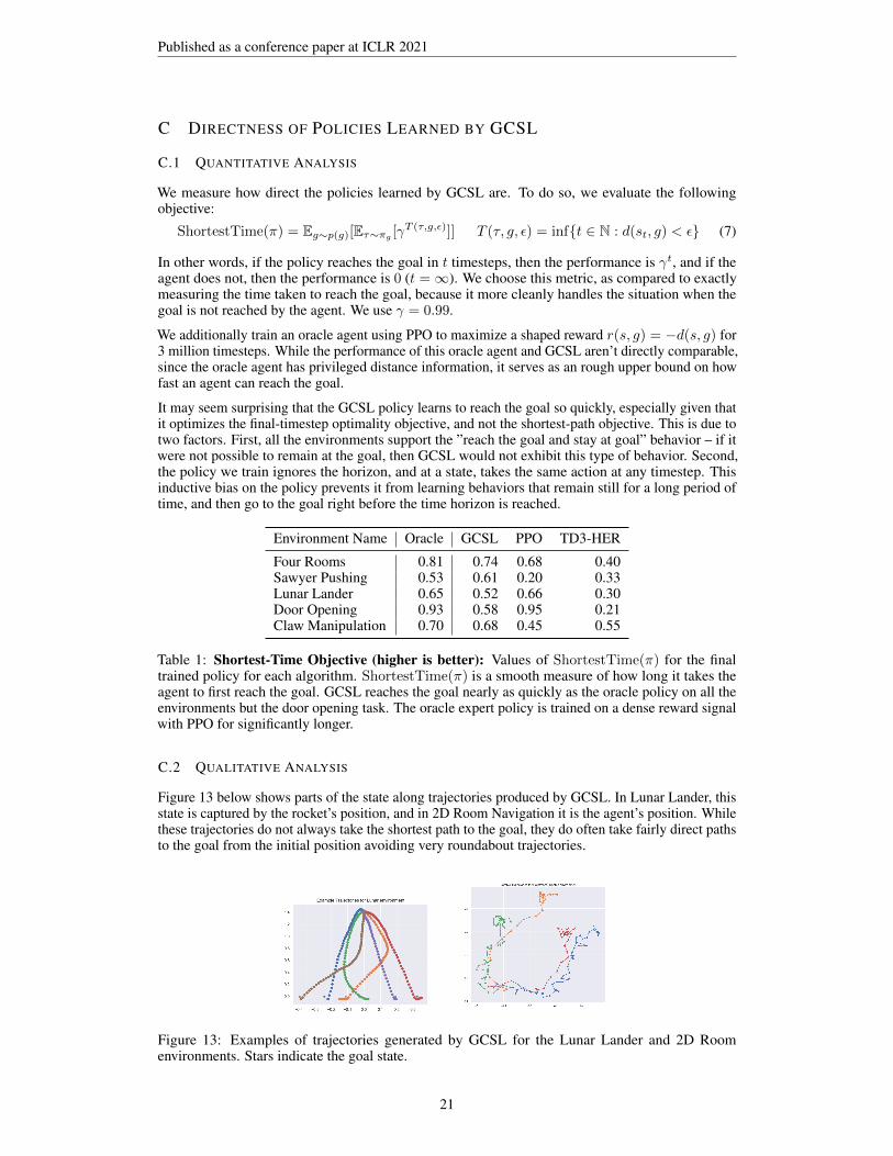
C.1 QUANTITATIVE ANALYSIS

We measure how direct the policies learned by GCSL are. To do so, we evaluate the followingobjective:

ShortestTime(π) = Eg∼p(g)[Eτ∼πg [γT (τ,g,ε)]] T (τ, g, ε) = inf{t ∈ N : d(st, g) < ε} (7)

In other words, if the policy reaches the goal in t timesteps, then the performance is γt, and if theagent does not, then the performance is 0 (t =∞). We choose this metric, as compared to exactlymeasuring the time taken to reach the goal, because it more cleanly handles the situation when thegoal is not reached by the agent. We use γ = 0.99.

We additionally train an oracle agent using PPO to maximize a shaped reward r(s, g) = −d(s, g) for3 million timesteps. While the performance of this oracle agent and GCSL aren’t directly comparable,since the oracle agent has privileged distance information, it serves as an rough upper bound on howfast an agent can reach the goal.

It may seem surprising that the GCSL policy learns to reach the goal so quickly, especially given thatit optimizes the final-timestep optimality objective, and not the shortest-path objective. This is due totwo factors. First, all the environments support the ”reach the goal and stay at goal” behavior – if itwere not possible to remain at the goal, then GCSL would not exhibit this type of behavior. Second,the policy we train ignores the horizon, and at a state, takes the same action at any timestep. Thisinductive bias on the policy prevents it from learning behaviors that remain still for a long period oftime, and then go to the goal right before the time horizon is reached.

Environment Name Oracle GCSL PPO TD3-HER

Four Rooms 0.81 0.74 0.68 0.40Sawyer Pushing 0.53 0.61 0.20 0.33Lunar Lander 0.65 0.52 0.66 0.30Door Opening 0.93 0.58 0.95 0.21Claw Manipulation 0.70 0.68 0.45 0.55

Table 1: Shortest-Time Objective (higher is better): Values of ShortestTime(π) for the finaltrained policy for each algorithm. ShortestTime(π) is a smooth measure of how long it takes theagent to first reach the goal. GCSL reaches the goal nearly as quickly as the oracle policy on all theenvironments but the door opening task. The oracle expert policy is trained on a dense reward signalwith PPO for significantly longer.

C.2 QUALITATIVE ANALYSIS

Figure 13 below shows parts of the state along trajectories produced by GCSL. In Lunar Lander, thisstate is captured by the rocket’s position, and in 2D Room Navigation it is the agent’s position. Whilethese trajectories do not always take the shortest path to the goal, they do often take fairly direct pathsto the goal from the initial position avoiding very roundabout trajectories.

Figure 13: Examples of trajectories generated by GCSL for the Lunar Lander and 2D Roomenvironments. Stars indicate the goal state.

21

learning to reach goals via iterated supervised …

Documents